TTP18–037, ZU-TH-39/18

November 2018

$\bm{D^{\ast}}$ polarization vs. $\bm{R_{D^{(\ast)}}}$ anomalies
in the leptoquark models

Syuhei Iguro^(a), Teppei Kitahara^(b,c,d,e,f), Yuji Omura^(c),
Ryoutaro Watanabe^(g), and Kei Yamamoto^(h,i)

^(a)Department of Physics, Nagoya University, Nagoya 464-8602, Japan

^(b)Institute for Advanced Research, Nagoya University, Furo-cho Chikusa-ku, Nagoya, Aichi, 464-8602 Japan

^(c)Kobayashi-Maskawa Institute for the Origin of Particles and the Universe,
Nagoya University, Nagoya 464-8602, Japan

^(d)Institute for Theoretical Particle Physics (TTP), Karlsruhe Institute of Technology, Engesserstraße 7, D-76128 Karlsruhe, Germany

^(e)Institute for Nuclear Physics (IKP), Karlsruhe Institute of Technology, Hermann-von-Helmholtz-Platz 1, D-76344 Eggenstein-Leopoldshafen, Germany

^(f)Physics Department, Technion–Israel Institute of Technology, Haifa 3200003, Israel

^(g)INFN, Sezione di Roma Tre, 00146 Rome, Italy

^(h)Physik-Institut, Universität Zürich, CH-8057 Zürich, Switzerland

⁽ⁱ⁾Graduate School of Science, Hiroshima University, Higashi-Hiroshima 739-8526, Japan

Polarization measurements in $\kern 1.79993pt\overline{\kern-1.79993ptB}{}\to D^{(\ast)}\tau\overline{\nu}$ are useful to check consistency in new physics explanations for the $R_{D}$ and $R_{D^{\ast}}$ anomalies. In this paper, we investigate the $D^{\ast}$ and $\tau$ polarizations and focus on the new physics contributions to the fraction of a longitudinal $D^{\ast}$ polarization ($F_{L}^{D^{\ast}}$), which is recently measured by the Belle collaboration $F_{L}^{D^{\ast}}=0.60\pm 0.09$, in model-independent manner and in each single leptoquark model (${\rm R}_{2}$, ${\rm S}_{1}$ and ${\rm U}_{1}$) that can naturally explain the $R_{D^{(\ast)}}$ anomalies. It is found that $\mathcal{B}(B_{c}^{+}\to\tau^{+}\nu)$ severely restricts deviation from the Standard Model (SM) prediction of $F_{L,\,\textrm{SM}}^{D^{\ast}}=0.46\pm 0.04$ in the leptoquark models: $[0.43,0.44]$, $[0.42,0.48]$, and $[0.43,0.47]$ are predicted as a range of $F_{L}^{D^{\ast}}$ for the ${\rm R}_{2}$, ${\rm S}_{1}$, and ${\rm U}_{1}$ leptoquark models, respectively, where the current data of $R_{D^{(\ast)}}$ is satisfied at $1\,\sigma$ level. It is also shown that the $\tau$ polarization observables can much deviate from the SM predictions. The Belle II experiment, therefore, can check such correlations between $R_{D^{(\ast)}}$ and the polarization observables, and discriminate among the leptoquark models.

1 Introduction

Semi-leptonic $B$ meson decays have been investigated to test the Standard Model (SM) since the CLEO, BaBar, and Belle experiments were established. In the processes, the SM predicts the specific flavor structure: the quark mixing is suppressed by the Cabbibo-Kobayashi-Maskawa (CKM) matrix elements [1, 2] and the dependence on the lepton flavor in the final state is universal in the predictions. Therefore, steady efforts have been made to measure them with high accuracy. The measurements are significant for not only the test of the SM but also probing New Physics (NP).

On recent years, the semi-tauonic processes, $\kern 1.79993pt\overline{\kern-1.79993ptB}{}\to D^{(\ast)}\tau\overline{\nu}$, have come under the spotlight since the BaBar [3, 4], Belle [5, 6, 7] and LHCb [8, 9] experiments have shown discrepancies between their data and the SM predictions in the measurements of

$$R_{D}=\frac{\mathcal{B}(\kern 1.79993pt\overline{\kern-1.79993ptB}{}\rightarrow D\tau\bar{\nu})}{\mathcal{B}(\kern 1.79993pt\overline{\kern-1.79993ptB}{}\rightarrow D\ell\bar{\nu})}\,,~{}~{}~{}~{}R_{D^{*}}=\frac{\mathcal{B}(\kern 1.79993pt\overline{\kern-1.79993ptB}{}\rightarrow D^{*}\tau\bar{\nu})}{\mathcal{B}(\kern 1.79993pt\overline{\kern-1.79993ptB}{}\rightarrow D^{*}\ell\bar{\nu})}\,,$$ (1.1)

where $\ell=e,\mu$.

The current situation on the experimental values and the SM predictions are summarized in Ref. [10] as $R_{D}^{\textrm{exp}}=0.407\pm 0.046$, $R_{D^{\ast}}^{\textrm{exp}}=0.306\pm 0.015$, $R_{D}^{\textrm{SM}}=0.299\pm 0.003$, and $R_{D^{\ast}}^{\textrm{SM}}=0.258\pm 0.005$. Hence the combined deviation is now $3.8\,\sigma$, referred to as $R_{D^{(*)}}$ anomalies. The surprising fact is that these decay processes are described by the tree-level amplitude in the SM and thus such a large discrepancy implies large unknown effects in the processes.

Motivated by those results, a lot of studies have been done from different points of view: re-evaluations of the form factors in the SM predictions, studies to accommodate the $R_{D^{(*)}}$ anomalies in NP models, and utilities of other observables than $R_{D^{(*)}}$ to probe NP effects. An overview of the above points, based on recent developments, can be summarized as follows:

• For the SM predictions, the heavy quark effective theory (HQET) has been applied to the form factors of the $\kern 1.79993pt\overline{\kern-1.79993ptB}{}\rightarrow D^{(*)}$ transitions [11]. In Refs. [12, 13], $\mathcal{O}(\Lambda_{\text{QCD}}/M_{Q})$ and $\mathcal{O}(\alpha_{s})$ corrections to the form factors in HQET are obtained. In Refs. [14, 15], another approach has been considered by taking the Boyd-Grinstein-Lebed parameterization [16]. Both of the two approaches enable us to evaluate the SM values with 1% level of the uncertainties as shown above. In Ref. [17], corrections from soft-photon effects are calculated and then one finds that it gives up to $3\,\text{--}\,4\%$ amplification of $R_{D}^{\textrm{SM}}$.

• The NP studies are summarized below:

  • One possible NP candidate to explain this anomaly was a charged scalar boson [18, 19, 20, 21, 22, 23, 24, 25, 26, 27, 28, 29, 30, 31, 32, 33, 34]. Regardless of the detail of the model, however, it has been turned out that this kind of scenario (i.e., with scalar mediator) becomes inconsistent with the bound from the $B_{c}^{+}$ lifetime [35, 36, 37, 26, 38]. It is also found that the direct search for $\tau\nu$ resonance at the LHC gives a bound which could be more stringent depending on the mass and the branching ratio of the charged scalar boson [39].

  • A charged vector boson ($W^{\prime}$) could be in this game [40, 41, 42, 44, 43, 45, 46, 47]. In order to introduce such a new vector field, we need additional gauge symmetry, which also leads to an additional neutral vector boson ($Z^{\prime}$) in general. With this additional ingredient, one can discuss a correlation between $\kern 1.79993pt\overline{\kern-1.79993ptB}{}\rightarrow D^{(*)}\tau\bar{\nu}$ and other processes such as $B\to K^{(*)}\mu^{+}\mu^{-}$.

  • A scalar or vector boson that couples to a quark and lepton pair [58], namely leptoquark (LQ), is another candidate as will be discussed in detail later. It has been already pointed out that three types of LQ models can accommodate the $R_{D^{(*)}}$ anomalies [59].

• Other observables of $\kern 1.79993pt\overline{\kern-1.79993ptB}{}\rightarrow D^{(*)}\tau\bar{\nu}$ have been examined in order to probe/distinguish NP effects/scenarios. At the coming Belle II experiment, a large amount of signal events will be available and thus distributions of the processes would be useful for this purpose. In Refs.[60, 61], it is pointed out that $5\,\text{ab}^{-1}$ data of the $q^{2}=(p_{B}-p_{D^{(*)}})^{2}$ distribution expected at the Belle II can distinguish some NP scenarios that can explain the present $R_{D^{(*)}}$ anomalies. The polarizations of $\tau$ and $D^{*}$ are also good candidates to test the NP scenarios [62, 63]. They reflect the spin structure of the interaction in $\kern 1.79993pt\overline{\kern-1.79993ptB}{}\rightarrow D^{(*)}\tau\bar{\nu}$, and could be affected by NP, e.g., see Refs.[62, 63, 59, 64, 65, 66, 67]. Relations between the $R_{D^{(*)}}$ anomalies and $|V_{cb}|$ determination with a tensor operator have also been discussed [68, 69, 70].

In this paper, we focus on the $D^{*}$ polarization following the new observation from the Belle experiment in which their first preliminary result of the longitudinal polarization $F_{L}^{D^{*}}$ has been given as [71]

$$F_{L}^{D^{\ast}}=0.60\pm 0.08({\rm stat.})\pm 0.035({\rm syst.}).$$ (1.2)

This is then compared with the SM prediction: $F_{L,\,\textrm{SM}}^{D^{\ast}}=0.46\pm 0.04$ [65]. Although they are consistent at $1.5\,\sigma$, the point here is that the experimental value is larger than the SM one. Indeed, this is an opposite correlation with the present $R_{D^{*}}$ anomaly in the presence of one NP effective operator for $b\to c\tau\nu$ as shown in Ref. [63] except for scalar NP scenarios.

In the light of this situation, we investigate relations among $R_{D}$, $R_{D^{\ast}}$, and $F_{L}^{D^{\ast}}$ in the LQ models that induce more than two effective operators, and see if they could accommodate the present data. We will begin with obtaining numerical formulae in terms of Wilson coefficients for NP operators by taking into account the recent development on the form factors. Then, we will show possible reaches of $F_{L}^{D^{\ast}}$ when we take into account the $R_{D^{(*)}}$ anomalies in the LQ models. We will also point out that the $\tau$ polarizations are useful to distinguish the LQ models based on sensitivities expected at the Belle II experiment.

This paper is organized as follows. In Sec. 2, we put the numerical formulae for the relevant observables in terms of the effective Hamiltonian. We also summarize the case for single operator analysis. In Sec. 3, based on the generic study with renormalization-group running effects, we obtain relations among $R_{D}$, $R_{D^{\ast}}$, and $F_{L}^{D^{\ast}}$ in the LQ models and discuss their potential to explain the present data. Relations to the $\tau$ polarizations are also discussed. Finally, we conclude our study in Sec. 4.

2 Formulae for the observables

At first, we describe general NP contributions in terms of the effective Hamiltonian. The operators relevant to $\kern 1.79993pt\overline{\kern-1.79993ptB}{}\to D^{(\ast)}\tau\overline{\nu}$ are described as

$${\cal{H}}_{\rm{eff}}=\frac{4G_{F}}{\sqrt{2}}V_{cb}\biggl{[}(1+C_{V_{1}})O_{V_{1}}+C_{V_{2}}O_{V_{2}}+C_{S_{1}}O_{S_{1}}+C_{S_{2}}O_{S_{2}}+C_{T}O_{T}\biggl{]},$$ (2.1)

at the scale $\mu=\mu_{b}=4.2\,\text{GeV}$ with

$$O_{V_{1}} =(\overline{c}\gamma^{\mu}P_{L}b)(\overline{\tau}\gamma_{\mu}P_{L}\nu_{\tau}),~{}~{}~{}O_{V_{2}}=(\overline{c}\gamma^{\mu}P_{R}b)(\overline{\tau}\gamma_{\mu}P_{L}\nu_{\tau}),$$

$$O_{S_{1}} =(\overline{c}P_{R}b)(\overline{\tau}P_{L}\nu_{\tau}),~{}~{}~{}~{}~{}~{}~{}~{}~{}\,O_{S_{2}}=(\overline{c}P_{L}b)(\overline{\tau}P_{L}\nu_{\tau}),$$

$$O_{T} =(\overline{c}\sigma^{\mu\nu}P_{L}b)(\overline{\tau}\sigma_{\mu\nu}P_{L}\nu_{\tau}),$$ (2.2)

where $P_{L}=(1-\gamma_{5})/2$ and $P_{R}=(1+\gamma_{5})/2$. Note that the SM prediction is given by $C_{X}=0$ for $X=V_{1,2}$, $S_{1,2}$, and $T$ in this description. We assume that the neutrino is always left-handed and third-generation ($\nu_{\tau}$). In LQ models, the neutrino flavor could be first- or second-generation ($\nu_{\mu,e}$) as seen in the next section. In principle, one can translate $C_{X}$ into that of $\nu_{\mu,\,e}$. Possibilities of the light sterile neutrinos are discussed in Refs. [30, 44, 45, 46, 47, 74, 75].

In this work, we follow analytic forms for the decay rates obtained in Refs. [59, 60]. As for all the form factors in both SM and NP amplitudes, we universally adopt the recent development taken in Ref. [12] such that a proper manner of the HQET expansion can be evaluated. To be precise, we have adopted the fit scenario “$\textrm{L}_{w\geq 1}+$SR” [12], where the HQET expansion is evaluated at the matching scale $\mu=\sqrt{m_{b}m_{c}}$ with QCD. According to Eq. (A5) of Ref. [12], we have evaluated observables at the scale $\mu=\mu_{b}$, as defined in the effective Hamiltonian of Eq. (2.1). In the end, we find the following numerical formulae

$$\frac{R_{D}}{R_{D}^{\textrm{SM}}}= ~{}|1+C_{V_{1}}+C_{V_{2}}|^{2}+1.02|C_{S_{1}}+C_{S_{2}}|^{2}+0.90|C_{T}|^{2}$$

$$+1.49\textrm{Re}[(1+C_{V_{1}}+C_{V_{2}})(C_{S_{1}}^{*}+C_{S_{2}}^{*})]+1.14\textrm{Re}[(1+C_{V_{1}}+C_{V_{2}})C_{T}^{*}]\,,$$ (2.3)

$$\frac{R_{D^{\ast}}}{R_{D^{\ast}}^{\textrm{SM}}}= ~{}|1+C_{V_{1}}|^{2}+|C_{V_{2}}|^{2}+0.04|C_{S_{1}}-C_{S_{2}}|^{2}+16.07|C_{T}|^{2}$$

$$-1.81\textrm{Re}[(1+C_{V_{1}})C_{V_{2}}^{*}]+0.11\textrm{Re}[(1+C_{V_{1}}-C_{V_{2}})(C_{S_{1}}^{*}-C_{S_{2}}^{*})]$$

$$-5.12\textrm{Re}[(1+C_{V_{1}})C_{T}^{*}]+6.66\textrm{Re}[C_{V_{2}}C_{T}^{*}]\,,$$ (2.4)

which can be compared with those in the recent literature [72, 45, 76]. Using our code, we obtained the SM predictions as $R_{D}^{\textrm{SM}}=0.300$ and $R_{D^{\ast}}^{\textrm{SM}}=0.256$, which are well consistent with Ref. [12].

Note that our values of $R_{D^{(\ast)}}$ and the following polarization observables are valid up to $\mathcal{O}(\Lambda_{\rm QCD}/m_{c,b})$ and $\mathcal{O}(\alpha_{s})$ within uncertainties from the input parameters [12]. We also emphasize that we have taken care of the scale for the Wilson coefficients and that for the HQET expansion to be $\mu=\mu_{b}=4.2\,\text{GeV}$. Although the SM operator is independent of such a scale, the NP operators do depend on it. For example, the coefficient of the $|C_{T}|^{2}$ term in $R_{D^{\ast}}/R_{D^{\ast}}^{\textrm{SM}}$ is found to be $17.24$ at the scale $\mu=\sqrt{m_{b}m_{c}}=2.6\,\text{GeV}$, whereas $16.07$ at $\mu=\mu_{b}=4.2\,\text{GeV}$ as shown in our result. This difference is indeed compensated with the running effect on the Wilson coefficient given as $C_{T}(\mu=2.6\,\text{GeV})=0.97\,C_{T}(\mu=4.2\,\text{GeV})$.

In a similar way, we can also calculate the polarizations in $\kern 1.79993pt\overline{\kern-1.79993ptB}{}\to D^{(\ast)}\tau\overline{\nu}$. The $D^{\ast}$ polarization is defined as the fraction of a longitudinal mode for the $D^{\ast}$ meson, namely,

$$F_{L}^{D^{\ast}} =\frac{\Gamma(\kern 1.79993pt\overline{\kern-1.79993ptB}{}\to D^{\ast}_{L}\tau\overline{\nu})}{\Gamma(\kern 1.79993pt\overline{\kern-1.79993ptB}{}\to D^{\ast}\tau\overline{\nu})}=\frac{\Gamma(\kern 1.79993pt\overline{\kern-1.79993ptB}{}\to D^{\ast}_{L}\tau\overline{\nu})}{\Gamma(\kern 1.79993pt\overline{\kern-1.79993ptB}{}\to D^{\ast}_{L}\tau\overline{\nu})+\Gamma(\kern 1.79993pt\overline{\kern-1.79993ptB}{}\to D^{\ast}_{T}\tau\overline{\nu})},$$ (2.5)

where $D^{\ast}_{L(T)}$ denotes the longitudinal (transverse) mode of the $D^{\ast}$ meson. For the numerical formula, we obtain

$${F_{L}^{D^{*}}\over F_{L,\,\textrm{SM}}^{D^{\ast}}}= \left({R_{D^{*}}\over R_{D^{*}}^{\text{SM}}}\right)^{-1}\!\!\!\times\Big{(}|1+C_{V_{1}}-C_{V_{2}}|^{2}+0.08|C_{S_{1}}-C_{S_{2}}|^{2}+7.02|C_{T}|^{2}$$

$$+0.24\textrm{Re}[(1+C_{V_{1}}-C_{V_{2}})(C_{S_{1}}^{*}-C_{S_{2}}^{*})]-4.37\textrm{Re}[(1+C_{V_{1}}-C_{V_{2}})C_{T}^{*}]\Big{)}.$$ (2.6)

Here the SM prediction is $F_{L,\,\textrm{SM}}^{D^{\ast}}=0.453$, which is consistent with Ref. [65].

For the $\tau$ polarization asymmetries along the longitudinal directions of the $\tau$ leptons in $\kern 1.79993pt\overline{\kern-1.79993ptB}{}\rightarrow D\tau\bar{\nu}$ and $\kern 1.79993pt\overline{\kern-1.79993ptB}{}\rightarrow D^{\ast}\tau\bar{\nu}$, we obtain

$${P_{\tau}^{D}\over P_{\tau,\,\textrm{SM}}^{D}}= \left({R_{D}\over R_{D}^{\text{SM}}}\right)^{-1}\!\!\!\times\Big{(}|1+C_{V_{1}}+C_{V_{2}}|^{2}+3.18|C_{S_{1}}+C_{S_{2}}|^{2}+0.18|C_{T}|^{2}$$

$$+4.65\textrm{Re}[(1+C_{V_{1}}+C_{V_{2}})(C_{S_{1}}^{*}+C_{S_{2}}^{*})]-1.18\textrm{Re}[(1+C_{V_{1}}+C_{V_{2}})C_{T}^{*}]\Big{)}\,,$$ (2.7)

and

$${P_{\tau}^{D^{\ast}}\over P_{\tau,\,\textrm{SM}}^{D^{\ast}}}= \left({R_{D^{\ast}}\over R_{D^{\ast}}^{\text{SM}}}\right)^{-1}\!\!\!\times\Big{(}|1+C_{V_{1}}|^{2}+|C_{V_{2}}|^{2}-0.07|C_{S_{1}}-C_{S_{2}}|^{2}-1.86|C_{T}|^{2}$$

$$-1.77\textrm{Re}[(1+C_{V_{1}})C_{V_{2}}^{\ast}]-0.22\textrm{Re}[(1+C_{V_{1}}-C_{V_{2}})(C_{S_{1}}^{*}-C_{S_{2}}^{*})]$$

$$-3.37\textrm{Re}[(1+C_{V_{1}})C_{T}^{*}]+4.37\textrm{Re}[C_{V_{2}}C_{T}^{*}]\Big{)},$$ (2.8)

respectively. The definitions of $P_{\tau}^{D}$ and $P_{\tau}^{D^{\ast}}$ are given in Refs. [63, 78]. Based on the present framework for the form factors, we obtain the SM predictions as $P_{\tau,\,\textrm{SM}}^{D}=0.320$ and $P_{\tau,\,\textrm{SM}}^{D^{\ast}}=-0.507$. Note that the polarizations are measurable by analyzing angular and/or energy distributions, e.g., see Refs. [62, 65]. For comparison, $P_{\tau,\,\textrm{SM}}^{D}=0.325\pm 0.009$ and $P_{\tau,\,\textrm{SM}}^{D^{\ast}}=-0.497\pm 0.013$ are obtained in Ref. [7] (Belle estimation), while $P_{\tau,\,\textrm{SM}}^{D}=0.34\pm 0.03$ in Ref. [67].

Another significant observable for our study is the branching ratio of $B_{c}^{+}\to\tau^{+}\nu$. As shown in Refs. [35, 37, 26], the constraint on the $B_{c}^{+}$ lifetime can be translated to that on $\mathcal{B}(B^{+}_{c}\to\tau^{+}\nu)$ and then one finds that a large scalar NP effect is disfavored. We also take this bound into account by using the analytic formula shown in Ref. [79]:

$$\frac{\mathcal{B}(B^{+}_{c}\to\tau^{+}\nu)}{\mathcal{B}(B^{+}_{c}\to\tau^{+}\nu_{\tau})_{\textrm{SM}}} =\left|1+C_{V_{1}}-C_{V_{2}}+\frac{m_{B_{c}}^{2}}{m_{\tau}\left(\overline{m}_{b}+\overline{m}_{c}\right)}\left(C_{S_{1}}-C_{S_{2}}\right)\right|^{2}$$ (2.9)

$$=\left|1+C_{V_{1}}-C_{V_{2}}+4.33\left(C_{S_{1}}-C_{S_{2}}\right)\right|^{2},$$ (2.10)

where the $\overline{\textrm{MS}}$ quark masses $\overline{m}_{b,c}$ at scale $\mu_{b}$ are used [80]. The SM prediction is $0.023$.

2.1 Case for single NP operator

Here we review a model-independent study on the correlation between $R_{D^{(\ast)}}$ and $F_{L}^{D^{\ast}}$ in the presence of a single NP operator in Eq. (2.1) .

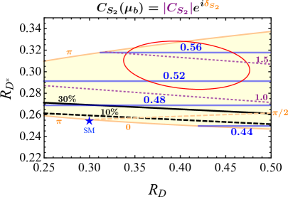
Figure 1: The contour for $F_{L}^{D^{\ast}}$ is shown with the blue line on the $R_{D}$–$R_{D^{\ast}}$ plane in the single NP operator scenario. The purple and orange lines represent the absolute value and the phase of $C_{X}(\mu_{b})$, respectively. The constraint from the $B_{c}^{+}$ lifetime is drawn by the solid (dashed) black line for $\mathcal{B}(B^{+}_{c}\to\tau^{+}\nu)<0.3$ (0.1). The world average of the data at $1\,\sigma$ ($2\,\sigma$) is shown by the red (dashed) ellipse. The SM point is represented by the blue star.

We parametrize $C_{X}$ $(X=V_{1},V_{2},S_{1},S_{2},T)$ as $C_{X}=|C_{X}|e^{i\delta_{X}}$, and then vary $|C_{X}|$ and $\delta_{X}$ (in the range of [0, $\pi$] for the latter). As for the $V_{1}$ case, $|C_{V_{1}}+1|$ is the only physical parameter and hence we take $C_{V_{1}}$ to be real for simplicity. In Fig. 1, the $F_{L}^{D^{\ast}}$ contour is shown with the blue line on the $R_{D}$–$R_{D^{\ast}}$ plane for each single operator: $O_{V_{1}}$, $O_{V_{2}}$, $O_{S_{1}}$, $O_{S_{2}}$, and $O_{T}$, where the shaded region in yellow is achievable with the NP operator and the red (dashed) ellipse stands for the world average of the present data at the $1\,\sigma$ ($2\,\sigma$) level [10]. In the plots, we also put some contours for $|C_{X}|$ and $\delta_{X}$ in purple and orange, respectively. The constraint from the $B_{c}^{+}$ lifetime is shown with the solid black and dashed black lines for $\mathcal{B}(B^{+}_{c}\to\tau^{+}\nu)<0.3$ and $<0.1$, respectively.

Note that charged scalar ($H^{\pm}$) scenario gives rise to non-zero $C_{S_{1,2}}$. A vector boson ($W^{\prime\pm}_{L}$) that couples to left-handed fermions contributes to $C_{V_{1}}$.

The vector operators ($O_{V_{1,2}}$) can explain the $R_{D^{(\ast)}}$ anomalies, but $F_{L}^{D^{\ast}}$ has to be the same as the SM prediction ($F_{L,\,\textrm{SM}}^{D^{\ast}}\simeq 0.45$). For the scalar operators ($O_{S_{1,2}}$), we can see that the constraint from the $B_{c}^{+}$ lifetime is significant and thus the deviations of $R_{D^{\ast}}$ and $F_{L}^{D^{\ast}}$ from their SM predictions are severely constrained. Finally, $F_{L}^{D^{\ast}}$ is suppressed as $R_{D^{(\ast)}}$ are enhanced in the case of the tensor operator $(O_{T})$.

3 Leptoquark scenarios

In this section, we discuss LQ models that can explain the $R_{D^{(\ast)}}$ anomalies, based on the generic analysis in Sec. 2. We address the following three types of LQs with (SU(3$)_{C}$, SU(2$)_{L}$, U(1$)_{Y})$ SM quantum numbers that are known as good candidates to accommodate the $R_{D^{(\ast)}}$ discrepancies:

• ${\rm R}_{2}$ with ($\bf{3},~{}\bf{2},~{}\frac{7}{6}$): SU(2$)_{L}$ doublet scalar LQ
  The scalar LQ ${\rm R}_{2}$ can generate significant contributions to $R_{D^{(\ast)}}$ (e.g., see Refs. [63, 81, 59]). ${\rm R}_{2}$ does not cause the proton decay since there is no diquark coupling. On the other hand, it is known that this scenario is not accessible to the $b\to s\mu\mu$ anomaly at the tree-level. The loop-level contributions [82] and the scenario with ${\rm R}_{2}$–${\rm S}_{3}$ combination [83] have been studied to accommodate both anomalies, where ${\rm S}_{3}$ with $({\bar{\bf 3}},{\bf 3},\frac{1}{3})$ is a SU(2$)_{L}$ triplet scalar LQ.

• ${\rm S}_{1}$ with ($\bf{\bar{3}},~{}\bf{1},~{}\frac{1}{3}$): SU(2$)_{L}$ singlet scalar LQ
  The scalar LQ ${\rm S}_{1}$ is also known as a candidate to explain the $R_{D^{(\ast)}}$ anomalies (e.g., see Refs. [59, 84, 36]). In order to ensure the proton stability, we assume that diquark couplings to LQ are forbidden (by a symmetry, see Ref. [85]). Although this LQ does not provide $b\to s\ell\ell$ transition at the tree-level, the loop-level contributions have been investigated[86]. Then it is found that the scenario with a pair of ${\rm S}_{1}$ and ${\rm S}_{3}$ is viable[87, 88, 89].

• ${\rm U}_{1}$ with ($\bf{3},~{}\bf{1},~{}\frac{2}{3}$): SU(2$)_{L}$ singlet vector LQ
  The ${\rm U}_{1}$ vector LQ has been receiving attention because it can provide a simultaneous explanation of the anomalies in the $b\to s$ and $b\to c$ transitions (e.g., see Refs. [90, 88, 91, 92, 93]). This LQ does not predict the proton decay.

3.1 Models

We adopt the notation of Refs. [85, 73]. The left-handed doublets are represented as $Q^{i}=\left((V_{\textrm{CKM}}^{\dagger}u_{L})^{i},\ d_{L}^{i}\right)^{T}$ and $L^{i}=\left({\nu_{L}^{i}},\ \ell_{L}^{i}\right)^{T}$, where $V_{\textrm{CKM}}$ is the CKM matrix. Here, $u^{i}$ and $d^{i}$ denote mass eigenstates. Below, we present the relevant couplings in the each model and derive the effective four-fermi interactions that contribute to the semi-leptonic $B$ decays.

3.1.1 ${\rm R}_{2}$ LQ model

We introduce one ${\rm R}_{2}$ LQ whose SM charges are ($\bf{3},~{}\bf{2},~{}\frac{7}{6}$). ${\rm R}_{2}$ is a scalar field, so that it couples to quarks and leptons flavor-dependently via Yukawa couplings. The Yukawa interactions involving ${\rm R}_{2}$ can be written as

$$\mathcal{L}_{{\rm R}_{2}}=y_{R}^{ij}\,\overline{Q}_{i}\ell_{R\,j}\,{\rm R}_{2}-y_{L}^{ij}\,\overline{u}_{R\,i}{{\rm R}_{2}}i\tau_{2}L_{j}+\mathrm{h.c.}\,,$$ (3.1)

where $y_{L}$ and $y_{R}$ are $3\times 3$ complex matrices. In terms of the electric charge eigenstates, it can be written as

$$\begin{split}\mathcal{L}_{{\rm R}_{2}}&=(V_{\textrm{CKM}}y_{R})^{ij}\,\overline{u}_{L\,i}\ell_{R\,j}\,{\rm R}_{2}^{(5/3)}+y_{R}^{ij}\,\overline{d}_{L\,i}\ell_{R\,j}\,{\rm R}_{2}^{(2/3)}\\[3.99994pt] &+y_{L}^{ij}\bar{u}_{R\,i}\nu_{L\,j}\,{\rm R}_{2}^{(2/3)}-y_{L}^{ij}\overline{u}_{R\,i}\ell_{L\,j}\,{\rm R}_{2}^{(5/3)}+\mathrm{h.c.}\end{split}$$ (3.2)

The superscripts of ${\rm R}_{2}$ denote the electromagnetic charges of the LQs. The ${\rm R}^{(2/3)}_{2}$ exchange gives contributions to $b\to c\tau{\bar{\nu}_{\tau}}$ at the tree-level, and generates the coefficients of the scalar and tensor operators at the scale $\mu=\mu_{\rm LQ}$:

$$C_{S_{2}}(\mu_{\rm LQ})=4\,C_{T}(\mu_{\rm LQ})=\dfrac{1}{4\sqrt{2}G_{F}V_{cb}}\dfrac{y_{L}^{c\tau}\big{(}y_{R}^{b\tau}\big{)}^{\ast}}{m_{R_{2}}^{2}}\,.$$ (3.3)

Assuming the Yukawa couplings are aligned to avoid the strong constraints from flavor observables, sizable $y_{L}^{c\tau}$ and $y_{R}^{b\tau}$ couplings can achieve the experimental results of $R_{D^{(\ast)}}$. For instance, when one chooses $y_{L}^{c\tau}(y_{R}^{b\tau})^{\ast}=2.5i$ and $m_{\textrm{LQ}}=1.5\ {\rm TeV}$, we have $C_{S_{2}}$ $(4C_{C_{T}})=0.41i$ that can explain the present $R_{D^{(\ast)}}$ data within $1\,\sigma$.

3.1.2 ${\rm S}_{1}$ LQ model

Next, we consider a ${\rm S}_{1}$ LQ whose SM charges are ($\bf{\bar{3}},~{}\bf{1},~{}\frac{1}{3}$). ${\rm S}_{1}$ is a SU(2)_L-singlet scalar, so the Yukawa couplings between ${\rm S}_{1}$ and the SM fermions can be written as

$$\begin{split}\mathcal{L}_{{\rm S}_{1}}&=y_{L}^{ij}\,\overline{Q^{C}}i\tau_{2}L_{j}\,{\rm S}_{1}+y_{R}^{ij}\,\overline{u^{C}_{R\,i}}e_{R\,j}\,{\rm S}_{1}+\mathrm{h.c.}\\[3.99994pt] &={\rm S}_{1}\Big{[}\big{(}V_{\textrm{CKM}}^{\ast}y_{L}\big{)}^{ij}\,\overline{u^{C}_{L\,i}}\ell_{L\,j}-y_{L}^{ij}\,\overline{d^{C}_{L\,i}}\nu_{L\,j}+y_{R}^{ij}\,\overline{u^{C}_{R\,i}}\ell_{R\,j}\Big{]}+\mathrm{h.c.}\,,\end{split}$$ (3.4)

where $y_{L}$ and $y_{R}$ are generic $3\times 3$ matrices. Assuming that $S_{1}$ is heavy, the contribution of the $S_{1}$ exchange to $b\to c\tau{\bar{\nu}_{\tau}}$ at the tree-level is given by

$$C_{V_{1}}(\mu_{\rm LQ}) =\dfrac{1}{4\sqrt{2}G_{F}V_{cb}}\dfrac{y_{L}^{b\tau}\big{(}V_{\textrm{CKM}}y_{L}^{\ast}\big{)}^{c\tau}}{m_{S_{1}}^{2}}\,,$$ (3.5)

$$C_{S_{2}}(\mu_{\rm LQ}) =-4\,C_{T}(\mu_{\rm LQ})=-\dfrac{1}{4\sqrt{2}G_{F}V_{cb}}\dfrac{y_{L}^{b{\tau}}\big{(}y_{R}^{c\tau}\big{)}^{\ast}}{m_{S_{1}}^{2}}\,.$$

Compared to the ${\rm R}_{2}$ case, $C_{V_{1}}$ is also generated. When one chooses $y_{L}^{b\tau}(V_{\textrm{CKM}}y_{L}^{\ast})^{c\tau}=0.3,~{}y_{L}^{b\tau}(y_{R}^{c\tau})^{\ast}=-0.3$ and $m_{\textrm{LQ}}=1.5\ {\rm TeV}$, $C_{V_{1}}$ and $C_{S_{2}}$ $(-4C_{C_{T}})$ are $0.05$ at the LQ mass scale, that can explain the $R_{D^{(\ast)}}$ anomalies at $1\,\sigma$ level.

3.1.3 ${\rm U}_{1}$ LQ model

We also consider a SU(2)_L-singlet massive vector LQ, ${\rm U}_{1}$. The SM charges of ${\rm U}_{1}$ are defined as ($\bf{3},~{}\bf{1},~{}\frac{2}{3}$). This LQ is a massive vector field, so that it could be realized by the extension of the SM gauge symmetry. We do not mention the underlying theory, but we simply discuss the phenomenology introducing flavor-dependent couplings between ${\rm U}_{1}$ and the SM fermions. Then, the coupling between ${\rm U}_{1}$ and the SM fermions can be described by

$$\mathcal{L}_{{\rm U}_{1}}=x_{L}^{ij}\,\bar{Q}_{i}\gamma_{\mu}{\rm U}_{1}^{\mu}L_{j}+x_{R}^{ij}\,\bar{d}_{R\,i}\gamma_{\mu}{\rm U}_{1}^{\mu}\ell_{R\,j}+\mathrm{h.c.},$$ (3.6)

where $x_{L}^{ij}$ and $x_{R}^{ij}$ are $3\times 3$ complex matrices. Integrating out the heavy ${\rm U}_{1}$, the couplings contribute to $b\to c\tau\bar{\nu}_{\tau}$ via the following coefficients

$$C_{V_{1}}(\mu_{\rm LQ}) =\dfrac{\,\left(V_{\textrm{CKM}}x_{L}\right)^{c\tau}\left(x_{L}^{b\tau}\right)^{\ast}}{2\sqrt{2}G_{F}V_{cb}\,m_{U_{1}}^{2}},$$ (3.7)

$$C_{S_{1}}(\mu_{\rm LQ}) =-\dfrac{\left(V_{\textrm{CKM}}x_{L}\right)^{c\tau}\left(x_{R}^{b\tau}\right)^{\ast}}{\sqrt{2}G_{F}V_{cb}\,m_{U_{1}}^{2}}.$$ (3.8)

Note that the formula of $C_{S_{1}}$ is omitted in Ref. [73]. The $C_{V_{1}}$ contribution interferes with the SM contribution, so that it easily enhances $R_{D^{(\ast)}}$. On the other hand, $C_{V_{1}}$ does not affect the polarization, as shown in Sec. 2.1. When $(V_{\textrm{CKM}}x_{L})^{c\tau}(x_{L}^{b\tau})^{\ast}=0.15$, $(V_{\textrm{CKM}}x_{L})^{c\tau}(x_{R}^{b\tau})^{\ast}=-0.15$, and $m_{\textrm{LQ}}=1.5\ {\rm TeV}$ are taken, $C_{V_{1}}=0.05$ and $C_{S_{1}}=0.1$, and the $R_{D^{(\ast)}}$ anomalies can be explained at $1\,\sigma$ level. We show our results of the flavor physics in each model, in Sec. 3.3.

3.2 Renormalization-group running effects

As seen above, some of LQs give rise to contributions from more than two types of the operators. In such a case, it is necessary to consider renormalization-group (RG) evolution effects from the NP scale ($\mu_{\rm NP}$) to the effective Hamiltonian matching scale ($\mu_{b}$). Let us briefly summarize the RG corrections in this subsection.

The semi-leptonic vector and axial vector four-fermion operators do not evolve in QCD [94] and there are no operator mixings with the other operators which we consider [95], so that we deal with $O_{V_{1,2}}$ as scale independent operators: $C_{V_{1,2}}(\mu_{b})\simeq C_{V_{1,2}}(\mu_{\rm NP})$.

It is pointed out that a large operator mixing between $O_{S_{2}}$ and $O_{T}$ arises from the electroweak anomalous dimension [96] above the electroweak symmetry breaking scale ($\mu_{\rm EW}$). The RG evolution for the operators $C_{i}=\left\{C_{S_{1}},C_{S_{2}},C_{T}\right\}$ at the one-loop level [95, 97, 96, 72] is given as

$$\frac{dC_{i}(\mu)}{d\ln\mu}=\frac{1}{16\pi^{2}}\left[g_{s}(\mu)^{2}\gamma_{s}^{T}+\gamma_{w}^{T}(\mu)+y_{t}(\mu)^{2}\gamma^{T}_{t}\right]_{ij}C_{j}(\mu),$$ (3.9)

with

$$\gamma_{s}^{T} =\left\{\gamma_{S},\gamma_{S},\gamma_{T}\right\}_{\rm diag},$$ (3.10)

$$\gamma_{w}^{T}(\mu) =\begin{pmatrix}-\frac{8}{3}g^{\prime 2}(\mu)&0&0\\ 0&-\frac{11}{3}g^{\prime 2}(\mu)&18g^{2}(\mu)+30g^{\prime 2}(\mu)\\ 0&\frac{3}{8}g^{2}(\mu)+\frac{5}{8}g^{\prime 2}(\mu)&-3g^{2}(\mu)+\frac{2}{9}g^{\prime 2}(\mu)\end{pmatrix},$$ (3.11)

$$\gamma_{t}^{T} =\left\{0,1/2,1/2\right\}_{\rm diag},$$ (3.12)

where $\gamma_{S}=-6C_{F}=-8$ and $\gamma_{T}=2C_{F}=8/3$. We numerically solve the RG evolution in Eq. (3.9) from $\mu_{\rm NP}$ to $\mu_{\rm EW}=m_{Z}$ in our analysis.

On the other hand, below the electroweak scale, the RG evolution is dominated by the QCD contributions. Reference [96] gives a numerical solution for the RG evolution at the three-loop in QCD and the one-loop in QED as follows,

$$\begin{pmatrix}C_{S_{1}}(\mu_{b})\\ C_{S_{2}}(\mu_{b})\\ C_{T}(\mu_{b})\end{pmatrix}\simeq\begin{pmatrix}1.46&0&0\\ 0&1.46&-0.0177\\ 0&-0.0003&0.878\end{pmatrix}\begin{pmatrix}C_{S_{1}}(m_{Z})\\ C_{S_{2}}(m_{Z})\\ C_{T}(m_{Z})\end{pmatrix}.$$ (3.14)

When one considers the RG evolution at the three-loop level in QCD and the one-loop level in electroweak and QED mentioned above, one obtains [96] $C_{S_{2}}(\mu_{b})\simeq+8.1C_{T}(\mu_{b})$ [$C_{S_{2}}(\mu_{b})\simeq-8.5C_{T}(\mu_{b})$] when $C_{S_{2}}(\mu_{\text{NP}})=+4C_{T}(\mu_{\text{NP}})$ [$C_{S_{2}}(\mu_{\text{NP}})=-4C_{T}(\mu_{\text{NP}})$] at $\mu_{\text{NP}}=\mathcal{O}(1)\text{TeV}$. Therefore, the ratio of $C_{S_{2}}(\mu_{b})$ to $C_{T}(\mu_{b})$ in the case with $C_{S_{2}}(\mu_{\rm NP})=-4C_{T}(\mu_{\rm NP})$ is more amplified than in the case with $C_{S_{2}}(\mu_{\rm NP})=+4C_{T}(\mu_{\rm NP})$ at $\mu_{\text{NP}}=\mathcal{O}(1)\text{TeV}$.

3.3 Results

Here, we discuss whether $F_{L}^{D^{\ast}}$ could be enhanced in the LQ scenarios that can accommodate the current $R_{D^{(\ast)}}$ anomalies. Note that the present case is different from the scenarios with the single NP operator (see Sec. 2.1) in the sense that various NP operators are induced from the LQ interactions and thus contributions to the observables are non-trivial.

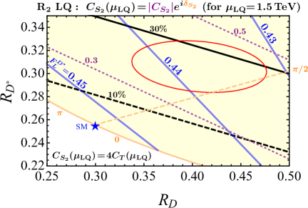
(a) ${\rm R}_{2}$ LQ

(b) ${\rm S}_{1}$ LQ with $C_{V_{1}}(\mu_{\textrm{LQ}})=0$

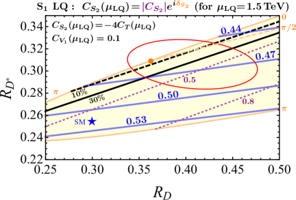
(c) ${\rm S}_{1}$ LQ with $C_{V_{1}}(\mu_{\textrm{LQ}})=0.1$

(d) ${\rm U}_{1}$ LQ with $C_{V_{1}}(\mu_{\textrm{LQ}})=0.1$

Figure 2: The $F_{L}^{D^{\ast}}$ contour is shown on the $R_{D}$–$R_{D^{\ast}}$ plane with the blue line in (a) ${\rm R}_{2}$, (b) ${\rm S}_{1}$ with $C_{V_{1}}=0$, (c) ${\rm S}_{1}$ with $C_{V_{1}}=0.1$ and (d) ${\rm U}_{1}$ with $C_{V_{1}}=0.1$ LQ scenarios at $m_{\rm LQ}=1.5\ {\rm TeV}$. The plot legend is the same as that in Fig. 1. The orange point stands for the case of $C_{S_{2}}=0$ and $C_{V_{1}}=0.1$ for the $\textrm{S}_{1}$ LQ or $C_{S_{1}}=0$ and $C_{V_{1}}=0.1$ for the $\textrm{U}_{1}$ LQ.

In Fig. 2, the $F_{L}^{D^{\ast}}$ contour is shown on the $R_{D}$–$R_{D^{\ast}}$ plane with the blue line in the three LQ models: ${\rm R}_{2}$, ${\rm S}_{1}$ and ${\rm U}_{1}$. We take $m_{\rm LQ}=1.5\,{\rm TeV}$ for a reference value of the LQ mass in our analysis, where the value is chosen so that the recent collider bounds are satisfied, e.g., see Ref. [73] for a review. Note that the LQ mass is relevant to the RG evolution effects and thus indicated in the plots. Then, the correlations among $R_{D}$, $R_{D^{\ast}}$, and $F_{L}^{D^{\ast}}$ are seen when varying the Wilson coefficients $C_{X}(\mu_{\rm LQ})$ in the complex plane. Here, we assume that the couplings of $y_{L,R}$ and $x_{L,R}$, relevant to $\kern 1.79993pt\overline{\kern-1.79993ptB}{}\to D^{(\ast)}\tau\overline{\nu}$, are sizable while the others are negligible in our analysis. In these plots, we focus on the parameter region that is favored by the $R_{D^{(\ast)}}$ experimental results.

Along with the $F_{L}^{D^{\ast}}$ contour, we also show the lines for the absolute value and phase of $C_{S_{1,2}}(\mu_{\rm LQ})\equiv|C_{S_{1,2}}|e^{i\delta_{S_{1,2}}}$ in purple and orange, respectively, in the figures. Note that the shaded region in yellow can be achieved in the single LQ scenario. The constraint from the $B_{c}^{+}$ lifetime is put with the solid (dashed) black lines corresponding to $\mathcal{B}(B^{+}_{c}\to\tau^{+}\nu)=0.3\ (0.1)$. The SM point and the present data for $R_{D^{(\ast)}}$ are denoted by the blue star and the red ellipse, respectively. The orange points stand for the cases of $C_{S_{2}}=0$ for the $\textrm{S}_{1}$ LQ and $C_{S_{1}}=0$ for the $\textrm{U}_{1}$ LQ.

In the ${\rm R}_{2}$ LQ model, the scalar Wilson coefficient $C_{S_{2}}$ and tensor one $C_{T}$ are introduced. In the Fig. 2(a), it is found that $F_{L}^{D^{\ast}}$ is not so changed from the SM point ($F_{L,\,\text{SM}}^{D^{\ast}}\simeq 0.45$) in this scenario. Our prediction of a range of $F_{L}^{D^{\ast}}$ within the present data of $R_{D^{(\ast)}}$ at $1\,\sigma$, and within the $B_{c}^{+}$ lifetime bound [$\mathcal{B}(B_{c}^{+}\to\tau^{+}\nu)<0.3$], is $[0.43,0.44]$. The value of $R_{D^{(\ast)}}$ is constrained by the $B_{c}^{+}$ lifetime. If we take $\mathcal{B}(B_{c}^{+}\to\tau^{+}\nu)<0.3$, $R_{D^{(\ast)}}$ is loosely constrained: the present data is still accommodated (with $|C_{S_{2}}(\mu_{{\rm LQ}})|=4|C_{T}(\mu_{{\rm LQ}})|\sim 0.4$ in the vicinity of $\delta_{S_{2}}=\pi/2$, for instance). The result is consistent with Refs. [81, 59, 98, 99].

In the ${\rm S}_{1}$ LQ model, the $C_{V_{1}}$, $C_{S_{2}}$, and $C_{T}$ operators are introduced with the relation as $C_{S_{2}}(\mu_{{\rm LQ}})=-4C_{T}(\mu_{{\rm LQ}})$. The phase of $C_{V_{1}}$ can be absorbed by the redefinition of $C_{S_{2},T}$ as shown in Appendix A, and thus only three parameters remain: $\delta_{S_{2}}$, $|C_{S_{2}}|$, and $|C_{V_{1}}|$. (Note that $C_{V_{1}}$ and $C_{S_{2}(T)}$ can be independent by using $y_{L}^{i\tau}$ and $y_{R}^{c\tau}$.) Then, the $F_{L}^{D^{\ast}}$ contour is shown for the cases of $|C_{V_{1}}|=0$ and $|C_{V_{1}}|=0.1$ in Fig. 2(b) and Fig. 2(c), respectively. It is found that a large $F_{L}^{D^{\ast}}$ is disfavored by the $B_{c}^{+}$ lifetime. The case for $|C_{V_{1}}|=0$ cannot explain the central value of the present $R_{D^{\ast}}$ data while that for $|C_{V_{1}}|=0.1$ can do [100]. We can see that the constraint $\mathcal{B}(B_{c}^{+}\to\tau^{+}\nu)<0.3$ is satisfied for the latter case. Finally, varying the value of $|C_{V_{1}}|$ we find that the ${\rm S}_{1}$ scenario predicts a range of $F_{L}^{D^{\ast}}$ as $[0.42,0.48]$.

In the ${\rm U}_{1}$ LQ model, the relevant Wilson coefficients are $C_{S_{1}}$ and $C_{V_{1}}$. In the same way as the ${\rm S}_{1}$ LQ, $|C_{V_{1}}|$, $|C_{S_{1}}|$, and $\delta_{S_{1}}$ are free parameters. The result for $|C_{V_{1}}|=0$ is the same as the one in one operator analysis $C_{S_{1}}$ in Fig. 1. The case for $|C_{V_{1}}|=0.1$ is shown in the Fig. 2(d). We find that the ${\rm U}_{1}$ LQ predicts a range of $F_{L}^{D^{\ast}}$ as $[0.43,0.47]$ and is consistent with the present data of $R_{D^{(\ast)}}$ and the bound of $\mathcal{B}(B_{c}^{+}\to\tau^{+}\nu)<0.3$.

(a) ${\rm R}_{2}$ LQ

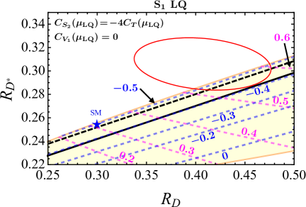
(b) ${\rm S}_{1}$ LQ with $C_{V_{1}}(\mu_{\textrm{LQ}})=0$

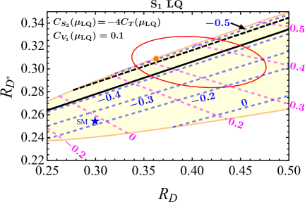
(c) ${\rm S}_{1}$ LQ with $C_{V_{1}}(\mu_{\textrm{LQ}})=0.1$

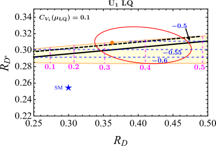
(d) ${\rm U}_{1}$ LQ with $C_{V_{1}}(\mu_{\textrm{LQ}})=0.1$

Figure 3: The contours of the $\tau$ polarizations $P_{\tau}^{D}$ and $P_{\tau}^{D^{\ast}}$ are shown on the $R_{D}$–$R_{D^{\ast}}$ plane in magenta and blue colors, respectively, when we consider the LQ scenarios of (a) ${\rm R}_{2}$, (b) ${\rm S}_{1}$ with $C_{V_{1}}=0$, (c) ${\rm S}_{1}$ with $C_{V_{1}}=0.1$ and (d) ${\rm U}_{1}$ with $C_{V_{1}}=0.1$. In all cases, $m_{\rm LQ}=1.5\ {\rm TeV}$ is taken. The SM point is represented by the blue star.

In the end, we found that these three LQ models cannot give $F_{L}^{D^{\ast}}$ deviating from the SM prediction ($F_{L,\,\text{SM}}^{D^{\ast}}\simeq 0.45$) as long as we take the present $R_{D^{(\ast)}}$ data seriously, especially a large deviation of $F_{L}^{D^{\ast}}$ is restricted by the severe constraint from the $B_{c}^{+}$ lifetime in the ${\rm S}_{1}$ and ${\rm U}_{1}$ models. Figure 2 shows that the LQ models can not explain the experimental result for $F_{L}^{D^{\ast}}$ in Eq. (1.2) at $1\,\sigma$ level. On the other hand, the large enhancement of $R_{D^{(\ast)}}$, compared with the SM predictions, is still possible although the severe constraint from the $B_{c}^{+}$ lifetime excludes some regions of the parameter space. Therefore, the large/small deviation of $R_{D^{(\ast)}}$/$F_{L}^{D^{\ast}}$ is one of the possibilities in the LQ models, which will be verified at the Belle II experiment. If this is the case, however, it is difficult to distinguish the LQ scenarios.

In turn, we study correlation between $R_{D^{(\ast)}}$ and the $\tau$ polarizations $P_{\tau}^{D^{(*)}}$. In Fig. 3, the contours of $P_{\tau}^{D}$ and $P_{\tau}^{D^{*}}$ are shown with dashed lines in magenta and blue, respectively. The other legends in the plots are the same as Fig. 2. We can see that each LQ model predicts unique ranges for $P_{\tau}^{D}$ and $P_{\tau}^{D^{\ast}}$, which can be used to distinguish these LQ models: $(P_{\tau}^{D},\,P_{\tau}^{D^{\ast}})$ with ([$0.42$, $0.57$], [$-0.44$, $-0.39$]) for ${\rm R}_{2}$ LQ, ([$0.11$, $0.63$], [$-0.51$, $-0.41$]) for ${\rm S}_{1}$ LQ and ([$0.23$, $0.52$], [$-0.57$,$-0.47$]) for ${\rm U}_{1}$ LQ are predicted where the current data of $R_{D^{(*)}}$ at $1\,\sigma$ and the bound of $\mathcal{B}(B_{c}^{+}\to\tau^{+}\nu)<0.3$ are satisfied. Here, $C_{V_{1}}(\mu_{\textrm{LQ}})$ is also varied in ${\rm S}_{1}$ and ${\rm U}_{1}$ LQ models. Note that the predicted ranges of $P_{\tau}^{D^{\ast}}$ are consistent with the latest result by the Belle experiment [7, 101]

$$P_{\tau}^{D^{\ast}}=-0.38\pm 0.51(\textrm{stat.}){}^{+0.21}_{-0.16}(\textrm{syst.}).$$ (3.17)

Since Belle II with $50\,{\rm ab}^{-1}$ data can measure $P_{\tau}^{D}$ with $3\%$ accuracy [67], and $P_{\tau}^{D^{\ast}}$ with $\pm 0.07$ [61], we point out that the future measurement of $P_{\tau}^{D}$ has sufficient sensitivity to distinguish between the LQ models. Note that $W^{\prime}$ models predict $P_{\tau}^{D}=P_{\tau,\,\textrm{SM}}^{D}$ for any values of $C_{V_{1}}$ and $C_{V_{2}}$. Thus, $P_{\tau}^{D}$ is a good observable for discrimination between $W^{\prime}$ and LQ models.

In Table 1, we summarize our results of the predictions on the polarization observables for the LQ models. This can be partly compared with Ref. [102] based on the SM effective field theory. Note that the uncertainties for the SM predictions are taken from Refs. [12, 65, 7]. We also stress that our study provides the theoretically possible ranges of the polarization observables which satisfy the current $R_{D^{(\ast)}}$ data at $1\,\sigma$ level, by scanning the full set of the parameters in the LQ models. On the other hand, model-independent and -dependent parameter fits from the data including $F_{L}^{D^{\ast}}$ are performed in Refs. [103, 76].

Table 1: Predicted ranges of the polarizations for ${\rm R}_{2}$, ${\rm S}_{1}$ and ${\rm U}_{1}$ LQ models ($\mu_{\textrm{LQ}}=1.5$ TeV), which satisfy the current $1\,\sigma$ data of $R_{D^{(*)}}$ and the bound of $\mathcal{B}(B_{c}^{+}\to\tau^{+}\nu)<0.3$. The SM predictions, the current data, and the expected sensitivity at Belle II with $50\,{\rm ab}^{-1}$ data [67, 61, 104] are also shown. The sensitivities for $F_{L}^{D^{\ast}}$ and $P_{\tau}^{D^{\ast}}$ are absolute uncertainty while the others are relative.

	$F_{L}^{D^{\ast}}$	$P_{\tau}^{D}$	$P_{\tau}^{D^{\ast}}$	$R_{D}$	$R_{D^{\ast}}$
${\rm R}_{2}$ LQ	[$0.43$, $0.44$]	[$0.42$, $0.57$]	[$-0.44$, $-0.39$]	$1\,\sigma$ data	$1\,\sigma$ data
${\rm S}_{1}$ LQ	[$0.42$, $0.48$]	[$0.11$, $0.63$]	[$-0.51$, $-0.41$]	$1\,\sigma$ data	$1\,\sigma$ data
${\rm U}_{1}$ LQ	[$0.43$, $0.47$]	[$0.23$, $0.52$]	[$-0.57$,$-0.47$]	$1\,\sigma$ data	$1\,\sigma$ data
SM	$0.46(4)$	$0.325(9)$	$-0.497(13)$	$0.299(3)$	$0.258(5)$
data	$0.60(9)$	-	$-0.38(55)$	$0.407(46)$	$0.306(15)$
Belle II	$0.04$	$3\%$	$0.07$	$3\%$	$2\%$

Before closing this section, we comment on the LQ mass dependence. Since there is no operator mixing, the figures for ${\rm U}_{1}$ LQ are independent of the LQ mass scale. Predicted ranges of $F_{L}^{D^{\ast}}$ and $P_{\tau}^{D^{(\ast)}}$ slightly depend on the LQ mass scale through the electroweak RG evolution in ${\rm R}_{2}$ and ${\rm S}_{1}$ LQ cases (see Sec. 3.2). We found that the variations of $F_{L}^{D^{\ast}}$ and $P_{\tau}^{D^{(\ast)}}$ are at the most $0.01$ when $1\,$TeV $<\mu_{\textrm{LQ}}<3\,$TeV is taken.

4 Conclusion

The observed excesses of $R_{D^{(\ast)}}$ in $\kern 1.79993pt\overline{\kern-1.79993ptB}{}\to D^{(\ast)}\tau\overline{\nu}$ have been one of the major anomalies in particle physics since the combined deviation is $3.8\,\sigma$ at present. Thus, it is important to summarize the NP explanations and investigate how to hunt the NP footprint. There are several ways to test the NP predictions according to the direct and indirect searches for NP signals. In fact, it is found that the $B_{c}^{+}$ lifetime severely constrains the NP scenarios, even though the leptonic decay, $B_{c}^{+}\to\tau^{+}\nu$, is still not directly observed. Moreover, it is recently pointed out that the direct search for the heavy resonance almost excludes the charged scalar scenario [39]. The measurements of the physical observables in $\kern 1.79993pt\overline{\kern-1.79993ptB}{}\to D^{(\ast)}\tau\overline{\nu}$ could also conclude the NP possibilities, as discussed in Refs. [62, 63, 59, 64, 65, 66, 67]. Recently, the Belle collaboration has reported the new result on the longitudinal $D^{\ast}$ polarization $F_{L}^{D^{\ast}}$ in $\kern 1.79993pt\overline{\kern-1.79993ptB}{}\to D^{\ast}\tau\overline{\nu}$, which could give us a new hint about the NP sector.

In this paper, we have investigated the correlations between the ratio $R_{D^{(\ast)}}$ and the $D^{*}$ polarization $F_{L}^{D^{\ast}}$ for the LQ models in terms of the general effective Hamiltonian. It is already known that the three types of LQs can easily explain the present $R_{D^{(\ast)}}$ anomalies; scalar LQs (${\rm R}_{2}$, ${\rm S}_{1}$) and vector LQ (${\rm U}_{1}$). Since the recent Belle result ($F_{L}^{D^{\ast}}=0.60\pm 0.09$) is slightly above the SM prediction ($F_{L,\,\text{SM}}^{D^{\ast}}\simeq 0.45$), the NP effect that enhances $F_{L}^{D^{\ast}}$ tends to be favored, which is not achievable with the single NP operators. Thus, we have tried to see if this could be possible in the LQ models that induce various types of NP operators. We, however, conclude that the possible deviations of $F_{L}^{D^{\ast}}$ from the SM prediction are small in the three LQ models. We find the predicted ranges of $F_{L}^{D^{\ast}}$ in the LQ models: $[0.43,0.44]$, $[0.42,0.48]$, and $[0.43,0.47]$ for ${\rm R}_{2}$, ${\rm S}_{1}$ and ${\rm U}_{1}$, respectively, in which the present $R_{D^{(\ast)}}$ anomaly can be explained within $1\,\sigma$. To be precise, it is found that $\mathcal{B}(B_{c}^{+}\to\tau^{+}\nu)$ severely restricts deviation of $F_{L}^{D^{\ast}}$ from the SM prediction in the ${\rm S}_{1}$ and ${\rm U}_{1}$ LQ models. In the ${\rm R}_{2}$ LQ case, $F_{L}^{D^{\ast}}$ is not much influenced. Therefore, it is unlikely to accommodate the present data of $R_{D^{(\ast)}}$ and $F_{L}^{D^{\ast}}$ simultaneously at $1\,\sigma$.

We also investigated the correlations between the $R_{D^{(\ast)}}$ explanation and the $\tau$ polarization asymmetries $P_{\tau}^{D^{(*)}}$ in the LQ models. It is found that the $\tau$ polarization observables can much deviate from the SM predictions.

In Table 1, predicted ranges of the polarizations for the LQ models are summarized. Then, we would point out that the upcoming Belle II experiment can survey the correlations between $R_{D^{(\ast)}}$ and the polarization observables with high accuracy enough to discriminate among the LQ models. Note that LHCb run II will also improve the $R_{D^{\ast}}$ observation [105]. According to our results, one can comment on a potential for future measurements of the polarization observables. As aforementioned in Sec. 1, the present data of $F_{L}^{D^{\ast}}$ is more than $1\,\sigma$ away from the SM prediction, although it still includes not small uncertainties. At present, the statistical error is dominant and this can be improved in the future measurement at the Belle II experiment [104]. Provided that the present systematic error still remains, it is found that ${\rm R}_{2}$, ${\rm S}_{1}$, and ${\rm U}_{1}$ LQ models are excluded at the $3\,\sigma$ level, if the present central value ($F_{L}^{D^{\ast}}\simeq 0.6$) is not changed. In the case, on the other hand, that data becomes consistent with the SM prediction ($F_{L}^{D^{\ast}}\simeq 0.46$), correlations between the other observables, $R_{D^{(\ast)}}$ and $P_{\tau}^{D^{(\ast)}}$, are significant to probe NP effects.

Appendix A Absorption of the phase of $C_{V_{1}}$

The global phase in (2.1) is unphysical and hence can be reabsorbed. In our numerical study, we have taken $C_{V_{1}}$ to be real by absorbing its phase as illustrated below.

In the ${\rm S}_{1}$ LQ model, the relevant Wilson coefficients are $C_{V_{1}},C_{S_{2}}$ and $C_{T}$. A general formula for relevant observables is given as a function of $(1+C_{V_{1}})$, $C_{S_{2}}$ and $C_{T}$

$$f\left(C_{V_{1}},\,C_{S_{2}},\,C_{T}\right)= a_{0}|1+C_{V_{1}}|^{2}+a_{1}|C_{S_{2}}|^{2}+a_{2}|C_{T}|^{2}+a_{3}\textrm{Re}[(1+C_{V_{1}})C_{S_{2}}^{\ast}]$$

$$+a_{4}\textrm{Re}[(1+C_{V_{1}})C_{T}^{\ast}]+a_{5}\textrm{Re}[C_{S_{2}}C_{T}^{\ast}],$$ (A.1)

where $a_{i}$ are real constants. Let us define $1+C_{V_{1}}\equiv C_{0}e^{i\theta_{0}}$ where $C_{0}$ is a real dimensionless number, then one obtains

$$f\left(C_{V_{1}},\,C_{S_{2}},\,C_{T}\right)= a_{0}C_{0}^{2}+a_{1}|C_{S_{2}}|^{2}+a_{2}|C_{T}|^{2}+a_{3}C_{0}\textrm{Re}[e^{i\theta_{0}}C_{S_{2}}^{\ast}]$$

$$+a_{4}C_{0}\textrm{Re}[e^{i\theta_{0}}C_{T}^{\ast}]+a_{5}\textrm{Re}[C_{S_{2}}C_{T}^{\ast}].$$ (A.2)

The phase $\theta_{0}$ can be absorbed by redefinitions of $C_{S_{2}}$ and $C_{T}$; $C_{S_{2}}\to C_{S_{2}}^{\prime}=C_{S_{2}}e^{-i\theta_{0}}$ and $C_{T}\to C_{T}^{\prime}=C_{T}e^{-i\theta_{0}}$. Besides, the LQ boundary condition $C_{S_{2}}(\mu_{\rm LQ})=-4C_{T}(\mu_{\rm LQ})$ and the RG evolution are compatible with the redefinitions. Therefore, the independent parameters are only three: $C_{0}$, $|C_{S_{2}}^{\prime}(\mu_{\rm LQ})|$ and Arg$\left[C_{S_{2}}^{\prime}(\mu_{\rm LQ})\right]$. This redefinition is also applicable for the case of the ${\rm U}_{1}$ LQ.

References

- [1] N. Cabibbo, “Unitary Symmetry and Leptonic Decays,” Phys. Rev. Lett. 10, 531 (1963).
- [2] M. Kobayashi and T. Maskawa, “ Violation in the Renormalizable Theory of Weak Interaction,” Prog. Theor. Phys. 49, 652 (1973).
- [3] J. P. Lees et al. [BaBar Collaboration], “Evidence for an excess of decays,” Phys. Rev. Lett. 109, 101802 (2012) [arXiv:1205.5442 [hep-ex]].
- [4] J. P. Lees et al. [BaBar Collaboration], “Measurement of an Excess of Decays and Implications for Charged Higgs Bosons,” Phys. Rev. D 88, no. 7, 072012 (2013) [arXiv:1303.0571 [hep-ex]].
- [5] M. Huschle et al. [Belle Collaboration], “Measurement of the branching ratio of relative to decays with hadronic tagging at Belle,” Phys. Rev. D 92, no. 7, 072014 (2015) [arXiv:1507.03233 [hep-ex]].
- [6] Y. Sato et al. [Belle Collaboration], “Measurement of the branching ratio of relative to decays with a semileptonic tagging method,” Phys. Rev. D 94, no. 7, 072007 (2016) [arXiv:1607.07923 [hep-ex]].
- [7] S. Hirose et al. [Belle Collaboration], “Measurement of the lepton polarization and in the decay ,” Phys. Rev. Lett. 118, no. 21, 211801 (2017) [arXiv:1612.00529 [hep-ex]].
- [8] R. Aaij et al. [LHCb Collaboration], “Measurement of the ratio of branching fractions ,” Phys. Rev. Lett. 115, no. 11, 111803 (2015) Erratum: [Phys. Rev. Lett. 115, no. 15, 159901 (2015)] [arXiv:1506.08614 [hep-ex]].
- [9] R. Aaij et al. [LHCb Collaboration], “Measurement of the ratio of the and branching fractions using three-prong -lepton decays,” Phys. Rev. Lett. 120, no. 17, 171802 (2018) [arXiv:1708.08856 [hep-ex]].
- [10] HFLAV average for Summer 2018, https://hflav-eos.web.cern.ch/hflav-eos/semi/summer18/RDRDs.html
- [11] I. Caprini, L. Lellouch and M. Neubert, “Dispersive bounds on the shape of anti- lepton anti-neutrino form-factors,” Nucl. Phys. B 530, 153 (1998) [hep-ph/9712417].
- [12] F. U. Bernlochner, Z. Ligeti, M. Papucci and D. J. Robinson, “Combined analysis of semileptonic decays to and : , , and new physics,” Phys. Rev. D 95, no. 11, 115008 (2017) Erratum: [Phys. Rev. D 97, no. 5, 059902 (2018)] [arXiv:1703.05330 [hep-ph]].
- [13] S. Jaiswal, S. Nandi and S. K. Patra, “Extraction of from and the Standard Model predictions of ,” JHEP 1712, 060 (2017) [arXiv:1707.09977 [hep-ph]].
- [14] D. Bigi and P. Gambino, “Revisiting ,” Phys. Rev. D 94, no. 9, 094008 (2016) [arXiv:1606.08030 [hep-ph]].
- [15] D. Bigi, P. Gambino and S. Schacht, “, , and the Heavy Quark Symmetry relations between form factors,” JHEP 1711, 061 (2017) [arXiv:1707.09509 [hep-ph]].
- [16] C. G. Boyd, B. Grinstein and R. F. Lebed, “Precision corrections to dispersive bounds on form-factors,” Phys. Rev. D 56, 6895 (1997) [hep-ph/9705252].
- [17] S. de Boer, T. Kitahara and I. Nisandzic, “Soft-Photon Corrections to Relative to ,” Phys. Rev. Lett. 120, no. 26, 261804 (2018) [arXiv:1803.05881 [hep-ph]].
- [18] A. Crivellin, C. Greub and A. Kokulu, “Explaining , and in a 2HDM of type III,” Phys. Rev. D 86, 054014 (2012) [arXiv:1206.2634 [hep-ph]].
- [19] A. Celis, M. Jung, X. Q. Li and A. Pich, “Sensitivity to charged scalars in and decays,” JHEP 1301, 054 (2013) [arXiv:1210.8443 [hep-ph]].
- [20] M. Tanaka and R. Watanabe, “New physics in the weak interaction of ,” Phys. Rev. D 87, no. 3, 034028 (2013) [arXiv:1212.1878 [hep-ph]].
- [21] P. Ko, Y. Omura and C. Yu, “ and in chiral U(1 models with flavored multi Higgs doublets,” JHEP 1303, 151 (2013) [arXiv:1212.4607 [hep-ph]].
- [22] A. Crivellin, A. Kokulu and C. Greub, “Flavor-phenomenology of two-Higgs-doublet models with generic Yukawa structure,” Phys. Rev. D 87, no. 9, 094031 (2013) [arXiv:1303.5877 [hep-ph]].
- [23] A. Crivellin, J. Heeck and P. Stoffer, “A perturbed lepton-specific two-Higgs-doublet model facing experimental hints for physics beyond the Standard Model,” Phys. Rev. Lett. 116, no. 8, 081801 (2016) [arXiv:1507.07567 [hep-ph]].
- [24] C. S. Kim, Y. W. Yoon and X. B. Yuan, “Exploring top quark FCNC within 2HDM type III in association with flavor physics,” JHEP 1512, 038 (2015) [arXiv:1509.00491 [hep-ph]].
- [25] J. M. Cline, “Scalar doublet models confront and anomalies,” Phys. Rev. D 93, no. 7, 075017 (2016) [arXiv:1512.02210 [hep-ph]].
- [26] A. Celis, M. Jung, X. Q. Li and A. Pich, “Scalar contributions to transitions,” Phys. Lett. B 771, 168 (2017) [arXiv:1612.07757 [hep-ph]].
- [27] P. Ko, Y. Omura, Y. Shigekami and C. Yu, “LHCb anomaly and B physics in flavored models with flavored Higgs doublets,” Phys. Rev. D 95, no. 11, 115040 (2017) [arXiv:1702.08666 [hep-ph]].
- [28] S. Iguro and K. Tobe, “ in a general two Higgs doublet model,” Nucl. Phys. B 925, 560 (2017) [arXiv:1708.06176 [hep-ph]].
- [29] K. Fuyuto, H. L. Li and J. H. Yu, “Implications of hidden gauged model for anomalies,” Phys. Rev. D 97, no. 11, 115003 (2018) [arXiv:1712.06736 [hep-ph]].
- [30] S. Iguro and Y. Omura, “Status of the semileptonic decays and muon in general 2HDMs with right-handed neutrinos,” JHEP 1805, 173 (2018) [arXiv:1802.01732 [hep-ph]].
- [31] S. Iguro, Y. Muramatsu, Y. Omura and Y. Shigekami, “Flavor physics in the multi-Higgs doublet models induced by the left-right symmetry,” arXiv:1804.07478 [hep-ph].
- [32] R. Martinez, C. F. Sierra and G. Valencia, “Beyond with the general 2HDM-III for ,” arXiv:1805.04098 [hep-ph].
- [33] S. Fraser, C. Marzo, L. Marzola, M. Raidal and C. Spethmann, “Towards a viable scalar interpretation of ,” Phys. Rev. D 98, no. 3, 035016 (2018) [arXiv:1805.08189 [hep-ph]].
- [34] S. P. Li, X. Q. Li, Y. D. Yang and X. Zhang, “ and neutrino mass in the 2HDM-III with right-handed neutrinos,” JHEP 1809, 149 (2018) [arXiv:1807.08530 [hep-ph]].
- [35] M. Beneke and G. Buchalla, “The Meson Lifetime,” Phys. Rev. D 53, 4991 (1996) [hep-ph/9601249].
- [36] X. Q. Li, Y. D. Yang and X. Zhang, “Revisiting the one leptoquark solution to the anomalies and its phenomenological implications,” JHEP 1608, 054 (2016) [arXiv:1605.09308 [hep-ph]].
- [37] R. Alonso, B. Grinstein and J. Martin Camalich, “Lifetime of Constrains Explanations for Anomalies in ,” Phys. Rev. Lett. 118, no. 8, 081802 (2017) [arXiv:1611.06676 [hep-ph]].
- [38] A. G. Akeroyd and C. H. Chen, “Constraint on the branching ratio of from LEP1 and consequences for anomaly,” Phys. Rev. D 96, no. 7, 075011 (2017) [arXiv:1708.04072 [hep-ph]].
- [39] S. Iguro, Y. Omura and M. Takeuchi, “Test of the anomaly at the LHC,” arXiv:1810.05843 [hep-ph].
- [40] X. G. He and G. Valencia, “ decays with leptons in nonuniversal left-right models,” Phys. Rev. D 87, no. 1, 014014 (2013) [arXiv:1211.0348 [hep-ph]].
- [41] A. Greljo, G. Isidori and D. Marzocca, “On the breaking of Lepton Flavor Universality in B decays,” JHEP 1507, 142 (2015) [arXiv:1506.01705 [hep-ph]].
- [42] S. M. Boucenna, A. Celis, J. Fuentes-Martin, A. Vicente and J. Virto, “Non-abelian gauge extensions for B-decay anomalies,” Phys. Lett. B 760, 214 (2016) [arXiv:1604.03088 [hep-ph]].
- [43] G. Cvetic, F. Halzen, C. S. Kim and S. Oh, “Anomalies in (semi)-leptonic decays , and , and possible resolution with sterile neutrino,” Chin. Phys. C 41, no. 11, 113102 (2017) [arXiv:1702.04335 [hep-ph]].
- [44] X. G. He and G. Valencia, “Lepton universality violation and right-handed currents in ,” Phys. Lett. B 779, 52 (2018) [arXiv:1711.09525 [hep-ph]].
- [45] P. Asadi, M. R. Buckley and D. Shih, “It’s all right(-handed neutrinos): a new W′ model for the anomaly,” JHEP 1809, 010 (2018) [arXiv:1804.04135 [hep-ph]].
- [46] A. Greljo, D. J. Robinson, B. Shakya and J. Zupan, “R(D(∗)) from W′ and right-handed neutrinos,” JHEP 1809, 169 (2018) doi:10.1007/JHEP09(2018)169 [arXiv:1804.04642 [hep-ph]].
- [47] K. S. Babu, B. Dutta and R. N. Mohapatra, “A Theory of Anomaly With Right-Handed Currents,” arXiv:1811.04496 [hep-ph].
- [48] R. Aaij et al. [LHCb Collaboration], “Test of lepton universality using decays,” Phys. Rev. Lett. 113, 151601 (2014) [arXiv:1406.6482 [hep-ex]].
- [49] R. Aaij et al. [LHCb Collaboration], “Test of lepton universality with decays,” JHEP 1708, 055 (2017) [arXiv:1705.05802 [hep-ex]].
- [50] R. Aaij et al. [LHCb Collaboration], “Measurement of Form-Factor-Independent Observables in the Decay ,” Phys. Rev. Lett. 111, 191801 (2013) [arXiv:1308.1707 [hep-ex]].
- [51] R. Aaij et al. [LHCb Collaboration], “Angular analysis of the decay using 3 fb-1 of integrated luminosity,” JHEP 1602, 104 (2016) [arXiv:1512.04442 [hep-ex]].
- [52] A. Abdesselam et al. [Belle Collaboration], “Angular analysis of ,” arXiv:1604.04042 [hep-ex].
- [53] The ATLAS collaboration [ATLAS Collaboration], “Angular analysis of decays in collisions at TeV with the ATLAS detector,” ATLAS-CONF-2017-023.
- [54] CMS Collaboration [CMS Collaboration], “Measurement of the and angular parameters of the decay in proton-proton collisions at ,” CMS-PAS-BPH-15-008.
- [55] R. Aaij et al. [LHCb Collaboration], “Differential branching fraction and angular analysis of the decay ,” JHEP 1307, 084 (2013) [arXiv:1305.2168 [hep-ex]].
- [56] R. Aaij et al. [LHCb Collaboration], “Angular analysis and differential branching fraction of the decay ,” JHEP 1509, 179 (2015) [arXiv:1506.08777 [hep-ex]].
- [57] J. Kumar, D. London and R. Watanabe, “Combined Explanations of the and Anomalies: a General Model Analysis,” arXiv:1806.07403 [hep-ph].
- [58] W. Buchmuller, R. Ruckl and D. Wyler, “Leptoquarks in Lepton - Quark Collisions,” Phys. Lett. B 191, 442 (1987) Erratum: [Phys. Lett. B 448, 320 (1999)].
- [59] Y. Sakaki, M. Tanaka, A. Tayduganov and R. Watanabe, “Testing leptoquark models in ,” Phys. Rev. D 88, no. 9, 094012 (2013) [arXiv:1309.0301 [hep-ph]].
- [60] Y. Sakaki, M. Tanaka, A. Tayduganov and R. Watanabe, “Probing New Physics with distributions in ,” Phys. Rev. D 91, no. 11, 114028 (2015) [arXiv:1412.3761 [hep-ph]].
- [61] E. Kou et al. [Belle II Collaboration], “The Belle II Physics Book,” arXiv:1808.10567 [hep-ex].
- [62] M. Tanaka and R. Watanabe, “Tau longitudinal polarization in tau nu and its role in the search for charged Higgs boson,” Phys. Rev. D 82, 034027 (2010) [arXiv:1005.4306 [hep-ph]].
- [63] M. Tanaka and R. Watanabe, “New physics in the weak interaction of ,” Phys. Rev. D 87, no. 3, 034028 (2013) [arXiv:1212.1878 [hep-ph]].
- [64] R. Alonso, A. Kobach and J. Martin Camalich, “New physics in the kinematic distributions of ,” Phys. Rev. D 94, no. 9, 094021 (2016) [arXiv:1602.07671 [hep-ph]].
- [65] A. K. Alok, D. Kumar, S. Kumbhakar and S. U. Sankar, “ polarization as a probe to discriminate new physics in ,” Phys. Rev. D 95, no. 11, 115038 (2017) [arXiv:1606.03164 [hep-ph]].
- [66] M. A. Ivanov, J. G. Körner and C. T. Tran, “Probing new physics in using the longitudinal, transverse, and normal polarization components of the tau lepton,” Phys. Rev. D 95, no. 3, 036021 (2017) [arXiv:1701.02937 [hep-ph]].
- [67] R. Alonso, J. Martin Camalich and S. Westhoff, “Tau properties in from visible final-state kinematics,” Phys. Rev. D 95, no. 9, 093006 (2017) [arXiv:1702.02773 [hep-ph]].
- [68] P. Biancofiore, P. Colangelo and F. De Fazio, “On the anomalous enhancement observed in decays,” Phys. Rev. D 87, no. 7, 074010 (2013) [arXiv:1302.1042 [hep-ph]].
- [69] P. Colangelo and F. De Fazio, “Tension in the inclusive versus exclusive determinations of : a possible role of new physics,” Phys. Rev. D 95, no. 1, 011701 (2017) [arXiv:1611.07387 [hep-ph]].
- [70] P. Colangelo and F. De Fazio, “Scrutinizing and in search of new physics footprints,” JHEP 1806, 082 (2018) [arXiv:1801.10468 [hep-ph]].
- [71] Talk by K. Adamczyk on “ to semitauonic decays at Belle/Belle II” in CKM 2018, Heidelberg, Germany, 17-21 September 2018.
- [72] F. Feruglio, P. Paradisi and O. Sumensari, “Implications of scalar and tensor explanations of ,” arXiv:1806.10155 [hep-ph].
- [73] A. Angelescu, D. Bečirević, D. A. Faroughy and O. Sumensari, “Closing the window on single leptoquark solutions to the -physics anomalies,” arXiv:1808.08179 [hep-ph].
- [74] D. J. Robinson, B. Shakya and J. Zupan, “Right-handed Neutrinos and ,” arXiv:1807.04753 [hep-ph].
- [75] A. Azatov, D. Barducci, D. Ghosh, D. Marzocca and L. Ubaldi, “Combined explanations of B-physics anomalies: the sterile neutrino solution,” JHEP 1810, 092 (2018) [arXiv:1807.10745 [hep-ph]].
- [76] M. Blanke, A. Crivellin, S. de Boer, M. Moscati, U. Nierste, I. Nišandžić and T. Kitahara, “Impact of polarization observables and on new physics explanations of the anomaly,” arXiv:1811.09603 [hep-ph].
- [77] M. Jung and D. M. Straub, “Constraining new physics in transitions,” arXiv:1801.01112 [hep-ph].
- [78] P. Asadi, M. R. Buckley and D. Shih, “Asymmetry Observables and the Origin of Anomalies,” arXiv:1810.06597 [hep-ph].
- [79] R. Watanabe, “New Physics effect on in relation to the anomaly,” Phys. Lett. B 776, 5 (2018) [arXiv:1709.08644 [hep-ph]].
- [80] K. G. Chetyrkin, J. H. Kuhn and M. Steinhauser, “RunDec: A Mathematica package for running and decoupling of the strong coupling and quark masses,” Comput. Phys. Commun. 133, 43 (2000) [hep-ph/0004189].
- [81] I. Doršner, S. Fajfer, N. Košnik and I. Nišandžić, “Minimally flavored colored scalar in and the mass matrices constraints,” JHEP 1311, 084 (2013) [arXiv:1306.6493 [hep-ph]].
- [82] D. Bečirević and O. Sumensari, “A leptoquark model to accommodate and ,” JHEP 1708, 104 (2017) [arXiv:1704.05835 [hep-ph]].
- [83] I. Doršner, S. Fajfer and N. Košnik, “Leptoquark mechanism of neutrino masses within the grand unification framework,” Eur. Phys. J. C 77, no. 6, 417 (2017) [arXiv:1701.08322 [hep-ph]].
- [84] M. Freytsis, Z. Ligeti and J. T. Ruderman, “Flavor models for ,” Phys. Rev. D 92, no. 5, 054018 (2015) [arXiv:1506.08896 [hep-ph]].
- [85] I. Doršner, S. Fajfer, A. Greljo, J. F. Kamenik and N. Košnik, “Physics of leptoquarks in precision experiments and at particle colliders,” Phys. Rept. 641, 1 (2016) [arXiv:1603.04993 [hep-ph]].
- [86] M. Bauer and M. Neubert, “Minimal Leptoquark Explanation for the R , RK , and Anomalies,” Phys. Rev. Lett. 116, no. 14, 141802 (2016) [arXiv:1511.01900 [hep-ph]].
- [87] A. Crivellin, D. Müller and T. Ota, “Simultaneous explanation of R(D(∗)) and : the last scalar leptoquarks standing,” JHEP 1709, 040 (2017) [arXiv:1703.09226 [hep-ph]].
- [88] D. Buttazzo, A. Greljo, G. Isidori and D. Marzocca, “B-physics anomalies: a guide to combined explanations,” JHEP 1711, 044 (2017) [arXiv:1706.07808 [hep-ph]].
- [89] D. Marzocca, “Addressing the B-physics anomalies in a fundamental Composite Higgs Model,” JHEP 1807, 121 (2018) [arXiv:1803.10972 [hep-ph]].
- [90] B. Bhattacharya, A. Datta, J. P. Guévin, D. London and R. Watanabe, “Simultaneous Explanation of the and Puzzles: a Model Analysis,” JHEP 1701, 015 (2017) [arXiv:1609.09078 [hep-ph]].
- [91] L. Calibbi, A. Crivellin and T. Li, “A model of vector leptoquarks in view of the -physics anomalies,” arXiv:1709.00692 [hep-ph].
- [92] M. Blanke and A. Crivellin, “ Meson Anomalies in a Pati-Salam Model within the Randall-Sundrum Background,” Phys. Rev. Lett. 121, no. 1, 011801 (2018) [arXiv:1801.07256 [hep-ph]].
- [93] A. Crivellin, C. Greub, F. Saturnino and D. Müller, “Importance of Loop Effects in Explaining the Accumulated Evidence for New Physics in B Decays with a Vector Leptoquark,” arXiv:1807.02068 [hep-ph].
- [94] A. J. Buras, “Weak Hamiltonian, CP violation and rare decays,” hep-ph/9806471.
- [95] R. Alonso, E. E. Jenkins, A. V. Manohar and M. Trott, “Renormalization Group Evolution of the Standard Model Dimension Six Operators III: Gauge Coupling Dependence and Phenomenology,” JHEP 1404, 159 (2014) [arXiv:1312.2014 [hep-ph]].
- [96] M. González-Alonso, J. Martin Camalich and K. Mimouni, “Renormalization-group evolution of new physics contributions to (semi)leptonic meson decays,” Phys. Lett. B 772, 777 (2017) [arXiv:1706.00410 [hep-ph]].
- [97] E. E. Jenkins, A. V. Manohar and M. Trott, “Renormalization Group Evolution of the Standard Model Dimension Six Operators II: Yukawa Dependence,” JHEP 1401, 035 (2014) [arXiv:1310.4838 [hep-ph]].
- [98] G. Hiller, D. Loose and K. Schönwald, “Leptoquark Flavor Patterns & Decay Anomalies,” JHEP 1612, 027 (2016) [arXiv:1609.08895 [hep-ph]].
- [99] D. Bečirević, I. Doršner, S. Fajfer, N. Košnik, D. A. Faroughy and O. Sumensari, “Scalar leptoquarks from grand unified theories to accommodate the -physics anomalies,” Phys. Rev. D 98, no. 5, 055003 (2018) [arXiv:1806.05689 [hep-ph]].
- [100] Y. Cai, J. Gargalionis, M. A. Schmidt and R. R. Volkas, “Reconsidering the One Leptoquark solution: flavor anomalies and neutrino mass,” JHEP 1710, 047 (2017) [arXiv:1704.05849 [hep-ph]].
- [101] S. Hirose et al. [Belle Collaboration], “Measurement of the lepton polarization and in the decay with one-prong hadronic decays at Belle,” Phys. Rev. D 97, no. 1, 012004 (2018) [arXiv:1709.00129 [hep-ex]].
- [102] Q. Y. Hu, X. Q. Li and Y. D. Yang, “ Transitions in the Standard Model Effective Field Theory,” arXiv:1810.04939 [hep-ph].
- [103] J. Aebischer, J. Kumar, P. Stangl and D. M. Straub, “A Global Likelihood for Precision Constraints and Flavour Anomalies,” arXiv:1810.07698 [hep-ph].
- [104] K. Adamczyk, “Semitauonic B decays at Belle/Belle II,” arXiv:1901.06380 [hep-ex].
- [105] R. Aaij et al. [LHCb Collaboration], “Physics case for an LHCb Upgrade II - Opportunities in flavour physics, and beyond, in the HL-LHC era,” arXiv:1808.08865.