QCD Improved Matching for Semi-Leptonic $B$ Decays with Leptoquarks

Abstract

Leptoquarks (LQs) provide very promising solutions to the tensions between the experimental measurements and the SM predictions of $b\to s\ell^{+}\ell^{-}$ and $b\to c\tau\nu$ processes. In this case the LQ masses are in general at the TeV scale and they can thus be produced at high energy colliders and dedicated LHC searches are ongoing. While for LQ production and decay the $O(\alpha_{s})$ corrections have been known for a long time, the $O(\alpha_{s})$ corrections to the matching on 2-quark-2-lepton operators have not been calculated, yet. In this article we close this gap by computing the QCD corrections to the matching of LQ models on the effective SM Lagrangian for both scalar and vector LQs. We find an enhancement of the Wilson coefficients of vector operators with respect to the tree-level results of around 8 % (13 %) if they originate from scalar (vector) LQs. This softens the LHC bounds and increases the allowed parameter space of LQ models addressing the flavour anomalies.

I Introduction

Significant deviations from the SM predictions in $b\to s\mu^{+}\mu^{-}$ processes (above the $5\,\sigma$ level Capdevila et al. (2018)) and in $b\to c\tau\nu$ processes (at the 4 $\sigma$ level Amhis et al. (2017)) were observed in recent years. These observations strongly point towards the violation of lepton flavour universality in semileptonic $B$ decays, suggesting a possible connection between these two classes of decays. In this context leptoquarks (LQs) are natural candidates for an explanation, since they give tree-level effects to semi-leptonic processes while their contributions to other flavour observables (which in general agree very well with the SM) are loop-suppressed. In fact, LQs (including squarks in the R-parity violating MSSM) have been extensively employed to explain the anomalies in $b\to s\mu^{+}\mu^{-}$ Gripaios et al. (2015); Biswas et al. (2015); Sahoo and Mohanta (2015); Huang and Tang (2015); de Medeiros Varzielas and Hiller (2015); Päs and Schumacher (2015); Deppisch et al. (2016); Chen et al. (2016); Bečirević et al. (2016a); Hiller et al. (2016); Duraisamy et al. (2017); Barbieri et al. (2017); Bečirević and Sumensari (2017); Guo et al. (2018); Aloni et al. (2017); Cline (2018); Fajfer et al. (2018); Sahoo and Mohanta (2018); Hati et al. (2018); de Medeiros Varzielas and King (2018) or $b\to c\tau\nu$ Deshpande and Menon (2013); Tanaka and Watanabe (2013); Sakaki et al. (2013); Freytsis et al. (2015); Hati et al. (2016); Li et al. (2016); Zhu et al. (2016); Popov and White (2017); Deshpande and He (2017); Altmannshofer et al. (2017a); Kamali et al. (2018); Azatov et al. (2018a); Zhu et al. (2018); Hu et al. (2018) processes. Furthermore, they can even provide a common explanation Bhattacharya et al. (2015); Alonso et al. (2015); Calibbi et al. (2015); Fajfer and Košnik (2016); Greljo et al. (2015); Barbieri et al. (2016); Bauer and Neubert (2016); Boucenna et al. (2016); Das et al. (2016); Bhattacharya et al. (2017); Bečirević et al. (2016b); Sahoo et al. (2017); Crivellin et al. (2017); Cai et al. (2017); Chen et al. (2017); Doršner et al. (2017); Buttazzo et al. (2017); Di Luzio et al. (2017); Bordone et al. (2018a); Barbieri and Tesi (2018); Calibbi et al. (2017); Blanke and Crivellin (2018); Greljo and Stefanek (2018); Bordone et al. (2018b); Crivellin et al. (2018a); Marzocca (2018); Aydemir et al. (2018); Fayyazuddin et al. (2018); Matsuzaki et al. (2018); Alvarez et al. (2018); Bečirević et al. (2018); Kumar et al. (2018); Azatov et al. (2018b); Di Luzio et al. (2018); Faber et al. (2018); Biswas et al. (2018); Angelescu et al. (2018); Choi et al. (2018); Heeck and Teresi (2018).

Direct searches for LQs at the LHC have been performed Aaboud et al. (2017, 2018); Sirunyan et al. (2017, 2018); Collaboration (2018) and also projections for future colliders in the context of the above mentioned flavour anomalies have been investigated Allanach et al. (2018). For collider processes the QCD corrections to production and decay of LQs are known for a long time Plehn et al. (1997); Kramer et al. (1997, 2005) and have been improved to include NLO parton shower Mandal et al. (2016) or a large width Hammett and Ross (2015). Furthermore, in recent analyses correlating the $B$ anomalies to LHC searches Faroughy et al. (2017); Doršner et al. (2017); Doršner and Greljo (2018); Hiller et al. (2018); Monteux and Rajaraman (2018); Schmaltz and Zhong (2018) QCD corrections to production and/or decay were included. However, the analogous $\alpha_{s}$ corrections for LQ effects in the low energy observables (i.e. semi-leptonic $B$ decays), which should be taken into account for consistency, are still missing.

In this article we therefore compute the 1-loop QCD corrections to the matching of models with LQs on the effective 4-fermion SM Lagrangian. After establishing our conventions in the next section, we perform the computation both for scalar and vector leptoquarks in a general gauge for the gluon fields in Sec. III. Finally we examine the importance of the calculated effects and conclude.

Figure 1: Examples of Feynman diagrams in the full and in the effective theory. $G$ denotes the ghost contribution. Not shown are the vector LQ self-energy with a Goldstone and a gluon as well as the vertex correction for the VLQ.

II Setup

As a starting point we consider the following generic Lagrangian governing the couplings of scalar (vector) LQs $\Phi$ ($V_{\mu}$) of mass $M$ to leptons $\ell$ (charged leptons or neutrinos) and quarks $q$ (up or down type):

$$\begin{aligned} L_{q\ell}^{LQ}=&\bar{q}\left({{\Gamma_{L}^{S}}{P_{L}}+{\Gamma_{R}^{S}}{P_{R}}}\right)\ell{\Phi^{*}}+{\rm{h}}{\rm{.c}}{\rm{.}}\\ &+\bar{q}\left({{\Gamma_{L}^{V}}\gamma^{\mu}{P_{L}}+{\Gamma_{R}^{V}}\gamma^{\mu}{P_{R}}}\right)\ell{V^{*}_{\mu}}+{\rm{h}}{\rm{.c}}{\rm{.}}\,.\end{aligned}$$ (1)

Note that here we do not consider gauge invariance with respect to $SU(2)_{L}$ or $U(1)_{Y}$. This is possible for our purpose since these gauge symmetries are disjunct from $SU(3)_{c}$. We also do not explicitly include the possibility of charge conjugated fields because this again does not affect the calculation of the QCD corrections. We will come back to the issue of charge conjugation later when we discuss the phenomenological importance of our results.

Let us now define the effective Lagrangian containing only SM fields in the $\bar{q}\ell\bar{\ell}q$ basis, which we call “LQ basis”

$$\begin{aligned} L_{{\rm{eff}}}^{{\rm{LQ}}}&=\widetilde{C}_{S}^{AB}\widetilde{O}_{S}^{AB}+\widetilde{C}_{V}^{AB}\widetilde{O}_{V}^{AB}+\widetilde{C}_{T}^{A}\widetilde{O}_{T}^{A}\,,\\ \widetilde{O}_{S}^{AB}&=\bar{q}{P_{A}}\ell\bar{\ell}{P_{B}}q\,,\\ \widetilde{O}_{V}^{AB}&=\bar{q}{\gamma^{\mu}}{P_{A}}\ell\bar{\ell}{\gamma_{\mu}}{P_{B}}q\,,\\ \widetilde{O}_{T}^{A}&=\bar{q}{\sigma^{\mu\nu}}{P_{A}}\ell\bar{\ell}{\sigma_{\mu\nu}}{P_{A}}q\,,\end{aligned}$$ (2)

as well as the corresponding operators in the “SM basis” with $\bar{q}q\bar{\ell}\ell$ operators

$$\begin{aligned} L_{{\rm{eff}}}^{{\rm{SM}}}&=C_{S}^{AB}O_{S}^{AB}+C_{V}^{AB}O_{V}^{AB}+C_{T}^{A}O_{T}^{A}\,,\\ O_{S}^{AB}&=\bar{q}{P_{A}}q\bar{\ell}{P_{B}}\ell\,,\\ O_{V}^{AB}&=\bar{q}{\gamma^{\mu}}{P_{A}}q\bar{\ell}{\gamma_{\mu}}{P_{B}}\ell,\;\;\\ O_{T}^{A}&=\bar{q}{\sigma^{\mu\nu}}{P_{A}}q\bar{\ell}{\sigma_{\mu\nu}}{P_{A}}\ell\,.\end{aligned}$$ (3)

Here $A,B=L,R$ label the chiralities. Performing the tree-level matching we obtain in the LQ basis

$$\begin{aligned} \widetilde{C}_{S}^{LR}&=\frac{{{{\left|{{\Gamma_{L}^{S}}}\right|}^{2}}}}{{{M^{2}}}},\\ \widetilde{C}_{S}^{LL}&=\frac{{\Gamma_{L}^{S}}\Gamma_{R}^{S*}}{{{M^{2}}}}\,,\\ \widetilde{C}_{T}^{L}&=0\,,\\ \widetilde{C}_{V}^{LL}&=-\frac{{{{\left|{{\Gamma_{L}^{V}}}\right|}^{2}}}}{{{M^{2}}}}\,,\\ \widetilde{C}_{V}^{LR}&=-\frac{{{\Gamma_{L}^{V}}\Gamma_{R}^{V*}}}{{{M^{2}}}}\,,\end{aligned}$$ (4)

and the corresponding formula with $L\leftrightarrow R$. Using standard Fierz identities (see e.g. Fierz (1937); Nieves and Pal (2004))

$$\begin{aligned} C_{V}^{LL}&=\widetilde{C}_{V}^{LL}\!\!\!&=&-\frac{{{{\left|{{\Gamma_{L}^{V}}}\right|}^{2}}}}{{{M^{2}}}}\,,\\ C_{S}^{LR}&=-2\widetilde{C}_{V}^{RL}\!\!\!&=&2\frac{{\Gamma_{R}^{V}\Gamma_{L}^{V*}}}{{{M^{2}}}}\,,\\ C_{T}^{L}&=-\frac{1}{8}\widetilde{C}_{S}^{LL}\!\!\!&=&-\frac{{1}}{8}\frac{{\Gamma_{L}^{S}\Gamma_{R}^{S*}}}{{{M^{2}}}}\,,\\ C_{S}^{LL}&=-\frac{1}{2}\widetilde{C}_{S}^{LL}\!\!\!&=&-\frac{1}{2}\frac{{\Gamma_{L}^{S}\Gamma_{R}^{S*}}}{{{M^{2}}}}\,,\\ C_{V}^{LR}&=-\frac{1}{2}\widetilde{C}_{S}^{RL}\!\!\!&=&-\frac{1}{2}\frac{{{{\left|{\Gamma_{R}^{S}}\right|}^{2}}}}{{{M^{2}}}}\,,\end{aligned}$$ (5)

where we again do not show the results which are obtained by an interchange of chiralities $L\leftrightarrow R$.

III Calculation and Results

Let us now turn to the calculation of the QCD corrections to the Wilson coefficients. Here, the same procedure is applied as within the SM when integrating out the $W$ boson Buchalla et al. (1996) in order to determine the $\alpha_{s}$ corrections to Eq. (5). We performed the calculation, also with the help of FeynArts Hahn (2001) and FeynCalc Mertig et al. (1991), in dimensional regularization with naive anti-commuting $\gamma_{5}$.

We assume that the vector LQ (VLQ) is a gauge boson of an unspecified gauge group. Thus, its couplings (and the ones of the corresponding Goldstone bosons) to gluons and ghosts are determined uniquely by requiring $SU(3)_{c}$ gauge invariance and the corresponding Lagrangian which also contains the mass term of the VLQ with mass $M$ is given by Blumlein et al. (1997)

$${L_{\rm VLQ}^{\rm QCD}}=-\frac{1}{2}K_{\mu\nu}^{\alpha{\dagger}}K_{\alpha}^{\mu\nu}+i{g_{s}}V_{\mu}^{\alpha{\dagger}}T_{\alpha\beta}^{a}V_{\nu}^{\beta}G_{a}^{\mu\nu}+M^{2}V_{\mu}^{\alpha{\dagger}}V_{\alpha}^{\mu}\,,$$ (6)

with

$$K_{\mu\nu}^{\alpha}=\left({D_{\mu}^{\alpha\beta}V_{\nu\beta}-D_{\nu}^{\alpha\beta}V_{\mu\beta}}\right)\,.$$ (7)

Here, $D_{\mu}^{\alpha\beta}={\partial_{\mu}}{\delta^{\alpha\beta}}+i{g_{s}}T_{a}^{\alpha\beta}A_{\mu}^{a}$ is the covariant derivative with respect to QCD, $\alpha$ and $\beta$ are colour indices and $a$ labels the eight generators $T_{a}$ of $SU(3)_{c}$, $A_{\mu}^{a}$ are the gluon fields and $G_{a}^{\mu\nu}$ is the usual field-strength tensor of $SU(3)_{c}$. Therefore, the situation is very similar to the SM, where the couplings of the $W$ boson and its Goldstone to photons and ghosts are governed by the electromagnetic gauge symmetry (i.e. the electric charge of the $W$) and a knowledge of the whole SM gauge group is not necessary. Thus, the VLQ (and the corresponding ghosts) couples in the same way to gluons as the photon to the $W$ (and its ghosts) with the replacement $e\to-g_{s}T_{a}$.

As mentioned, the aim of this work is to calculate QCD corrections to the Wilson coefficients appearing in Eqs. (2) and (3). To fix the order $\alpha_{s}$ pieces of these coefficients, we calculate the scattering amplitude $A$ for the process $q\bar{\ell}\to q\bar{\ell}$ both in the full theory and in the effective theory. Within the full theory we have to calculate the following ingredients: the LQ self-energy, the box diagrams and the genuine vertex corrections (see Fig. 1). Within the effective theory we only have to calculate the genuine vertex correction.

Since the Wilson coefficients of our dimension six operators do not depend on the momenta and masses of the external particles, we put them to zero in our calculation. By doing so, we also avoid the generation of terms which correspond to operators of dimension higher than six. Similarly, this means that we also set the fermion masses in the couplings of Goldstone bosons to zero. Therefore, box diagrams or vertex corrections involving Goldstones vanish and merely their effect in the LQ self-energy remains. In our computational framework infrared (IR) divergences related to soft and collinear gluons are dimensionally regularized, manifesting themselves as $1/\varepsilon_{\rm IR}$ poles. For the gluon we use a general gauge with gauge parameter $\xi$ while for the vector LQ we use Feynman gauge (i.e. $\xi_{LQ}=1$).

In both the full and the effective theory we perform the necessary renormalizations leading to ultraviolet finite expressions for the amplitude $A$, from which we then can extract the QCD corrections to the Wilson coefficients.

We are aware of the fact that our calculation of the QCD corrections to the Wilson coefficients presented in the following subsections could be partially abbreviated at several places. For didactical reasons, however, we calculate the complete renormalized amplitude for both the full and the effective theory (for the very simple configuration of external states as stated above), mainly because we want to illustrate that the $\xi$-dependence drops out at the level of the renormalized amplitudes.

III.1 Calculation in the Full Theory

In the full theory the result for the $q\bar{\ell}\to q\bar{\ell}$ amplitude (discarding terms of order $1/M^{3}$ and higher) can be written in lowest order as

$$A_{\rm tree}^{S} =i\left(\!{\frac{{{{\left|{\Gamma_{L}^{S}}\right|}^{2}}}}{{{M^{2}}}}\langle\widetilde{O}_{S}^{LR}\rangle+\frac{{\Gamma_{L}^{S}\Gamma_{R}^{S*}}}{{{M^{2}}}}\langle\widetilde{O}_{S}^{LL}\rangle+L\leftrightarrow R{\mkern 1.0mu}}\!\right)\,,$$ (8)

$$A_{\rm tree}^{V} =i\left(\!-{\frac{{{{|\Gamma_{L}^{V}|^{2}}}}}{{{M^{2}}}}\langle\widetilde{O}_{V}^{LL}\rangle-\frac{{\Gamma_{L}^{V}\Gamma_{R}^{V*}}}{{{M^{2}}}}\langle\widetilde{O}_{V}^{LR}\rangle+L\leftrightarrow R{\mkern 1.0mu}}\!\right)\,,$$

for scalar and vector LQ exchange, respectively. The symbol $\langle\tilde{O}\rangle$ is a short-hand notation for the tree-level matrix element $\langle\bar{\ell}q|\tilde{O}|q\bar{\ell}\rangle$ associated with the operators in (2). In the following we calculate order $\alpha_{s}$ QCD corrections to this amplitude, discussing in turn the contributions due to the LQ self-energy, the vertex corrections and the box diagram.

We identify the corresponding self-energy diagram in Fig. 1 (with amputated external legs) with $-i\Sigma_{S}(p^{2})$ for scalar LQs. For working out its direct contribution to the amplitude $A$, we need $\Sigma_{S}$ at $p^{2}=0$. In our computation we also have to renormalize the mass $M$ of the leptoquark, which we do in the on-shell scheme. As the corresponding renormalization constant is directly related to $\Sigma_{S}(M^{2})$, we give the results at $p^{2}=M^{2}$ and at $p^{2}=0$, reading

$$\begin{aligned} \dfrac{\Sigma_{S}\left({{M^{2}}}\right)}{{M^{2}}}&=\frac{\alpha_{s}}{4\pi}{C_{F}}\left({\frac{3}{\varepsilon}+3l_{\mu}+7}\right)\,,\\ \dfrac{\Sigma_{S}\left(0\right)}{{M^{2}}}&=\frac{\alpha_{s}}{4\pi}{C_{F}}\xi\left({\frac{1}{\varepsilon}+l_{\mu}+1}\right)\,,\end{aligned}$$ (9)

with $l_{\mu}=\log(\mu^{2}/M^{2})$.

The combined effect of the direct contribution and the renomalization constant of the LQ mass leads to the occurrence of $\Sigma_{S}(M^{2})-\Sigma_{S}(0)$ at the level of the amplitude $A$. Therefore, we only kept self-energy bubble diagrams in the above expressions, i.e. all self-energy contributions which are not tadpoles, as the latter drop out in the difference.

For the vector LQ we identify the corresponding diagram with $+i\Sigma_{V}^{\mu\nu}$. In our computation we only need the part proportional to $+ig_{\mu\nu}$ which we denote as $\Sigma_{V}(p^{2})$. Again, the expressions for $p^{2}=0$ and $p^{2}=M^{2}$ are needed, reading

$$\begin{aligned} \dfrac{\Sigma_{V}\left({{M^{2}}}\right)}{M^{2}}\!\!&=\frac{\alpha_{s}}{36\pi}C_{F}\left(\frac{57}{\varepsilon}+57l_{\mu}+89\right)\,,\\ \dfrac{\Sigma_{V}\left(0\right)}{M^{2}}\!&=\frac{\alpha_{s}}{4\pi}C_{F}\left(\!\!\frac{(\xi+5)}{2}\left(\!\frac{1}{\varepsilon}+\!l_{\mu}\right)+\frac{(\xi\!+\!7)}{4}\!\right)\,.\end{aligned}$$ (10)

The vertex corrections lead to the following contribution to the amplitude

$$\begin{aligned} A^{S,V}_{\rm tree}\left(1+2\Lambda_{S,V}\right)\,,\end{aligned}$$ (11)

with

$$\Lambda_{S} =\frac{\alpha_{s}}{4\pi}{C_{F}}\xi\left({\frac{1}{\varepsilon}+l_{\mu}+1}\right)\,,$$ (12)

$$\Lambda_{V} =\frac{\alpha_{s}}{16\pi}C_{F}(\xi+3)\left(\frac{3}{\varepsilon}+3l_{\mu}+\frac{5}{2}\right)\,.$$ (13)

The box diagram contribution to the amplitudes can be compactly written as

$$\begin{aligned} \Delta_{S}&=\frac{\alpha_{s}}{4\pi}C_{F}\,k_{1}\,(1-\xi)\,A^{S}_{\rm tree}-\frac{i}{M^{2}}\frac{\alpha_{s}}{16\pi}{C_{F}}\,k_{2}\,\left[\,\left(\left|{\Gamma^{S}_{L}}\right|^{2}\langle\widetilde{O}_{2\gamma}^{LR}\rangle+{\Gamma_{L}^{S*}{\Gamma^{S}_{R}}\langle{\widetilde{O}}^{RR}_{2\gamma}\rangle}\right)+L\leftrightarrow R\right]\,,\\ \Delta_{V}&=\frac{\alpha_{s}}{4\pi}C_{F}\,k_{1}\,(1-\xi)\,A^{V}_{\rm tree}+\frac{i}{M^{2}}\frac{\alpha_{s}}{16\pi}{C_{F}}\,k_{2}\,\left[\,\left(\left|{\Gamma^{V}_{L}}\right|^{2}\langle\widetilde{O}_{3\gamma}^{LL}\rangle+{\Gamma_{L}^{V}{\Gamma^{V*}_{R}}\langle{\widetilde{O}}^{LR}_{3\gamma}\rangle}\right)+L\leftrightarrow R\right]\,,\end{aligned}$$ (14)

for scalar and vector LQs, respectively. The expressions for $k_{1}$ and $k_{2}$ read

$$k_{1} =\frac{1}{\varepsilon_{\rm IR}}+1+l_{\mu}\,,\qquad k_{2} =\frac{1}{\varepsilon_{\rm IR}}+\frac{3}{2}+l_{\mu}\,.$$ (15)

The symbols $\langle\widetilde{O}\rangle$ again denote the tree-level matrix elements of the operators $\widetilde{O}$ in (2). Furthermore, we defined

$$\begin{aligned} &&\langle\widetilde{O}^{AB}_{2\gamma}\rangle=\langle\bar{q}{\gamma^{\mu}}{\gamma^{\nu}}{P_{A}}\bar{\ell}\ell{\gamma_{\nu}}{\gamma_{\mu}}{P_{B}}q\rangle\,,\\ &&\langle\widetilde{O}^{AB}_{3\gamma}\rangle=\langle\bar{q}{\gamma^{\mu}}{\gamma^{\nu}}{\gamma^{\sigma}}{P_{A}}\bar{\ell}\ell{\gamma_{\sigma}}{\gamma_{\nu}}{\gamma_{\mu}}{P_{B}}q\rangle\,.\end{aligned}$$ (16)

In addition to the contributions of the various diagrams just described, we have to renormalize the coupling constants of the leptoquark to the fermions and we have to take into account the LSZ factor of the quark fields. Thereby the couplings get replaced by $\Gamma_{L,R}^{S,V}\to\Gamma_{L,R}^{S,V}\left({1+\delta\Gamma_{L,R}^{S,V}}\right)$ and the quark fields by $q\to q\left({1+\delta Z_{q}}\right)$. The explicit expressions read

$$\delta\Gamma_{L,R}^{S} =-\frac{\alpha_{s}}{4\pi}C_{F}\frac{3}{2}\frac{1}{\varepsilon}\,,\qquad\delta\Gamma_{L,R}^{V} =-\frac{\alpha_{s}}{4\pi}C_{F}\frac{25}{6}\frac{1}{\varepsilon}\,,$$ (17)

$$\delta Z_{q} =\frac{\alpha_{s}}{4\pi}C_{F}\,\xi\,\left(\frac{1}{\varepsilon_{\rm IR}}-\frac{1}{\varepsilon}\right)\,.$$

Note that we have already discussed (and taken into account) the renormalization of the mass of the LQ. The final renormalized results for the amplitudes in the full theory read

$$A_{\rm full,ren}^{S(V),\alpha_{s}} =\Delta_{S(V)}\!+\!\left({2\Lambda_{S(V)}+\dfrac{{\Sigma_{S,(V)}\left({{M^{2}}}\right)\!-\!\Sigma_{S(V)}\left(0\right)}}{{{M^{2}}}}}+\delta Z_{q}+2\delta\Gamma_{L,R}^{S(V)}\!\right)\,A^{S(V)}_{\rm tree}\,.$$ (18)

When inserting all the ingredients listed above into these formulas, we see that the ultraviolet singularities are cancelled. Also the $\xi$ dependence related to the gluon cancels in these expressions, as it should be the case when calculating on-shell matrix elements. Only $1/\varepsilon_{\rm IR}$ infrared singularities remain which will enter the corresponding matrix element in the effective theory in precisely the same way, leading to finite Wilson coefficients.

III.2 Effective Theory and Matching

Within the effective theory, we first calculate the QCD corrections to the amplitudes $q\bar{\ell}\to q\bar{\ell}$ originating from the operators in Eq. (2) (see last diagram in FIG. 1). We obtain

$$\begin{aligned} \Delta_{S}^{\rm eff}&=\frac{\alpha_{s}}{4\pi}C_{F}\left(\frac{1}{\varepsilon_{\rm IR}}-\frac{1}{\varepsilon}\right)\,(1-\xi)\,A^{S}_{\rm tree}-\frac{i}{M^{2}}\frac{\alpha_{s}}{16\pi}{C_{F}}\,\left(\frac{1}{\varepsilon_{\rm IR}}-\frac{1}{\varepsilon}\right)\,\left[\,\left(\left|{\Gamma^{S}_{L}}\right|^{2}\langle\widetilde{O}_{2\gamma}^{LR}\rangle+{\Gamma_{L}^{S*}{\Gamma^{S}_{R}}\langle{\widetilde{O}}^{RR}_{2\gamma}\rangle}\right)+L\leftrightarrow R\right]\,,\\ \Delta_{V}^{\rm eff}&=\frac{\alpha_{s}}{4\pi}C_{F}\,\left(\frac{1}{\varepsilon_{\rm IR}}-\frac{1}{\varepsilon}\right)\,(1-\xi)\,A^{V}_{\rm tree}+\frac{i}{M^{2}}\frac{\alpha_{s}}{16\pi}{C_{F}}\,\left(\frac{1}{\varepsilon_{\rm IR}}-\frac{1}{\varepsilon}\right)\,\left[\,\left(\left|{\Gamma^{V}_{L}}\right|^{2}\langle\widetilde{O}_{3\gamma}^{LL}\rangle+{\Gamma_{L}^{V}{\Gamma^{V*}_{R}}\langle{\widetilde{O}}^{LR}_{3\gamma}\rangle}\right)+L\leftrightarrow R\right]\,,\end{aligned}$$ (19)

for scalar and vector LQs, respectively. We immediately see that the $\xi$-dependence drops out when taking into account the effect of $\delta Z_{q}$. Furthermore, we observe that the infrared divergences are then the same as in the full theory. Since we are interested in the matching, we drop at this level all the terms involving $1/\varepsilon_{\rm IR}$ in both versions of the theory. We then rewrite

$$\widetilde{O}_{2\gamma}^{AB}=(4-2\varepsilon)\widetilde{O}_{S}^{AB}+\widetilde{O}_{T}^{AB}\,.$$ (20)

$\widetilde{O}_{T}^{AB}$ vanishes in $d=4$ dimensions for $A\neq B$. Therefore, it plays the role of an evanescent operator. For $A=B$ we have $\widetilde{O}_{T}^{AA}=\widetilde{O}_{T}^{A}$, where $\widetilde{O}_{T}^{A}$ is present in the operator basis.
Furthermore, we rewrite $\widetilde{O}_{3\gamma}^{AB}$ (see e.g. Ref. Chetyrkin et al. (1998)) as

$$\widetilde{O}_{3\gamma}^{LL} =\left({4-8\varepsilon}\right)\widetilde{O}_{V}^{LL}-\widetilde{O}_{E}^{LL}\,,$$ (21)

$$\widetilde{O}_{3\gamma}^{LR} =16\left({1-\varepsilon}\right)\widetilde{O}_{V}^{LR}-\widetilde{O}_{E}^{LR}\,,$$

where $\widetilde{O}_{E}^{LL}$ and $\widetilde{O}_{E}^{LR}$ are evanescent operators. Renormalizing the operators (including the evanescent ones) in the $\overline{\rm MS}$-scheme, we obtain (after dropping the infrared terms as described)

$$\begin{aligned} A_{\rm eff,ren}^{S,\alpha_{s}}=&-\frac{i}{M^{2}}\frac{\alpha_{s}}{8\pi}C_{F}\left[|\Gamma_{L}^{S}|^{2}\langle\widetilde{O}_{S}^{LR}\rangle+\Gamma_{L}^{S}\Gamma_{R}^{S*}\langle\widetilde{O}_{S}^{LL}\rangle\right]+i\delta\widetilde{C}_{S}^{LR}\langle\widetilde{O}_{S}^{LR}\rangle+i\delta\widetilde{C}_{S}^{LL}\langle\widetilde{O}_{S}^{LL}\rangle+i\delta\widetilde{C}_{T}^{R}\langle\widetilde{O}_{T}^{R}\rangle+(L\leftrightarrow R)\,,\\ A_{\rm eff,ren}^{V,\alpha_{s}}&=\frac{i}{M^{2}}\frac{\alpha_{s}}{2\pi}C_{F}\left[|\Gamma_{L}^{V}|^{2}\langle\widetilde{O}_{V}^{LL}\rangle+2\Gamma_{L}^{V}\Gamma_{R}^{V*}\langle\widetilde{O}_{V}^{LR}\rangle\right]+i\delta\widetilde{C}_{V}^{LL}\langle\widetilde{O}_{V}^{LL}\rangle+i\delta\widetilde{C}_{V}^{LR}\langle\widetilde{O}_{V}^{LR}\rangle+(L\leftrightarrow R)\,.\end{aligned}$$ (22)

The quantities $\delta C$ contain the order $\alpha_{s}$ corrections to the respective Wilson coefficients. The corresponding results in the full theory (also after dropping the infrared terms) read

$$A_{\rm full,ren}^{S,\alpha_{s}} =\frac{i}{M^{2}}\frac{\alpha_{s}}{4\pi}C_{F}\left(3l_{\mu}+\frac{13}{2}\right)\left[|\Gamma_{L}^{S}|^{2}\langle\widetilde{O}_{S}^{LR}\rangle+\,\Gamma_{L}^{S}\Gamma_{R}^{S*}\langle\widetilde{O}_{S}^{LL}\rangle\right]-\frac{i}{M^{2}}\frac{\alpha_{s}}{16\pi}C_{F}\left(l_{\mu}+\frac{3}{2}\right)\Gamma_{L}^{S*}\Gamma_{R}^{S}\langle\widetilde{O}_{T}^{R}\rangle+(L\leftrightarrow R)\,,$$

$$A_{\rm full,ren}^{V,\alpha_{s}} =-\frac{i}{M^{2}}\frac{\alpha_{s}}{72\pi}C_{F}\left[5\left(30l_{\mu}+41\right)|\Gamma_{L}^{V}|^{2}\langle\widetilde{O}_{V}^{LL}\rangle+4\left(24l_{\mu}+31\right)\Gamma_{L}^{V}\Gamma_{R}^{V*}\langle\widetilde{O}_{V}^{LR}\rangle\right]+(L\leftrightarrow R)\,.$$ (23)

From these equations the Wilson coefficients are easily determined, reading

$$\begin{aligned} \widetilde{C}^{LR}_{S}&=\frac{{\left|{\Gamma_{L}^{S}}\right|^{2}}}{{{M^{2}}}}\left({1+\frac{{{\alpha_{s}}}}{{4\pi}}C_{F}}\left({{\rm{3}}l_{\mu}{\rm{+7}}}\right)\right),\\ \widetilde{C}^{RR}_{S}&=\frac{{\Gamma_{R}^{S}\Gamma_{L}^{S*}}}{{{M^{2}}}}\left({1+\frac{{{\alpha_{s}}}}{{4\pi}}C_{F}}\left({{\rm{3}}l_{\mu}{\rm{+7}}}\right)\right),\\ {{\widetilde{C}}}^{R}_{T}&=-\frac{{\Gamma_{R}^{S}\Gamma_{L}^{S*}}}{{{M^{2}}}}\frac{{{\alpha_{s}}}}{{16\pi}}C_{F}\left({l_{\mu}{{+\frac{3}{2}}}}\right)\,,\\ {\widetilde{C}}^{LL}_{V}&=-\frac{{\left|{\Gamma_{L}^{V}}\right|^{2}}}{{{M^{2}}}}\left({1+\frac{{{\alpha_{s}}}}{{72\pi}}{{{C}}_{{F}}}\left({150l_{\mu}+241}\right)}\right)\,,\\ {\widetilde{C}}^{LR}_{V}&=-\frac{{\Gamma_{L}^{V}\Gamma_{R}^{V*}}}{{{M^{2}}}}\left({1+\frac{{{\alpha_{{s}}}}}{{18\pi}}{{{C}}_{{F}}}\left({24l_{\mu}+49}\right)}\right)\,,\end{aligned}$$ (24)

and the corresponding equations obtained by exchanging $L$ and $R$.

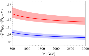
Figure 2: Left: Dependence of the Wilson coefficients of vector operators (in the SM basis) on a variation of the matching scale $\mu$ for $M=1\,{\rm TeV}$. Note that the ratio $C_{V}(\mu)/C_{V}(\mu=M)$ only depends very weakly on the overall scale $M$. One can clearly see that the scale dependence significantly reduces when going from LO to NLO. The $\mu$ dependence of the vector operator is bigger when generated by a VLQ rather than by a SLQ. Right: Ratio of the Wilson coefficient of vector operators calculated at NLO in $\alpha_{s}$ ($C_{V}^{\rm NLO}$) to the corresponding Wilson coefficient at leading order at $\mu=M$ ($C_{V}^{\rm LO}(\mu=M)$). The corresponding coloured regions indicate the remaining NLO matching scale uncertainties and are obtained by varying $\mu$ between $1/2M$ and $2M$.

Finally, we have to discuss the transition to the SM basis (Eq. (3)), in which the QCD running and the physical observables are calculated. A naive four-dimensional Fierz transformation is not applicable à priori at the one-loop level. Instead, we require that the renormalized matrix elements for the process $q\bar{\ell}\to q\bar{\ell}$ calculated in both versions of the effective theory coincide. Due to the specific definition of the evanescent operators (see (Eq. 21)), we obtain for the Wilson coefficients

$$\begin{aligned} C_{V}^{LL,RR}&=\widetilde{C}_{V}^{LL,RR}\,,\\ C_{S}^{LR,RL}&=-2\widetilde{C}_{V}^{RL,LR}\,,\end{aligned}$$ (25)

i.e., there are no corrections with respect to the 4-dimensional Fierz identities for vector LQs. However, for the operators generated by scalar LQs this is not the case and corrections to the naive Fierz identities do appear, as our results show:

$$\begin{aligned} C_{V}^{RL}&=-\frac{1}{2}\widetilde{C}_{S}^{LR}\left({1+\frac{3}{{8\pi}}{C_{F}}{\alpha_{s}}}\right)\,,\\ C_{S}^{LL}&=-\frac{1}{2}\widetilde{C}_{S}^{LL}\left({1+\frac{7}{{8\pi}}{C_{F}}{\alpha_{s}}}\right)-6\widetilde{C}_{T}^{L}\,,\\ C_{T}^{LL}&=-\frac{1}{8}\widetilde{C}_{S}^{LL}\left({1-\frac{1}{{8\pi}}{C_{F}}{\alpha_{s}}}\right)+\frac{1}{2}\widetilde{C}_{T}^{L}\,.\end{aligned}$$ (26)

At this point, we should remind the reader that the corrections for the vector LQs are independent of the gluon gauge parameter $\xi$ but depend on the LQ gauge parameter (which we set to 1 in Feynman gauge). This is an artefact of our simplified model framework for the vector LQ. In a UV complete model there will of course be additional contributions which are not taken into account in our analysis. However, also for collider analyses simplified models are used. Furthermore, since we calculate QCD corrections (and not LQ corrections) to the matching, the independence on the gluon gauge parameter is sufficient to justify that our results are reasonable. I.e. we calculated the minimal QCD matching effects which are present in any model and only get supplemented by additional effects depending on the UV completion.

IV Impact and Conclusions

The results of our calculation above can be summarized in the following compact way: In the SM basis, the lowest order Wilson coefficients of vector and scalar operators receive a shift

$$\begin{aligned} C_{V}^{\rm VLQ}\to C_{V}^{\rm VLQ}\left({1+\frac{{{\alpha_{s}}}}{{72\pi}}{{{C}}_{{F}}}\left({150l_{\mu}+241}\right)}\right)\,,\\ C_{S}^{\rm VLQ}\to C_{S}^{\rm VLQ}\left({1+\frac{{{\alpha_{{s}}}}}{{18\pi}}{{{C}}_{{F}}}\left({24l_{\mu}+49}\right)}\right)\,,\end{aligned}$$ (27)

if they originate from vector LQs. Concerning operators arising from scalar LQs we have

$$C_{V}^{\rm SLQ} \to C_{V}^{\rm SLQ}\left({1+\frac{{{\alpha_{s}}}}{{4\pi}}{C_{F}}\left({{\rm{3}}l_{\mu}{\rm{+}}\frac{{17}}{2}}\right)}\right)\,,$$

$$C_{S}^{\rm SLQ} \to C_{S}^{\rm SLQ}\left({1+\frac{{3{\alpha_{s}}}}{{2\pi}}{C_{F}}}\right)\,,$$ (28)

$$C_{T}^{\rm SLQ} \to C_{T}^{\rm SLQ}\left({1+\frac{{{\alpha_{s}}}}{\pi}{C_{F}}\left({l_{\mu}{\rm{+2}}}\right)}\right)\,,$$

for all Wilson coefficients of vector, scalar and tensor operators, respectively. Note that these formulas are valid for all 10 representations of scalar and vector LQs which have couplings invariant under the SM gauge group Buchmuller et al. (1987) to quarks and leptons and even apply if the LQ couples to right-handed neutrinos instead of SM leptons. They also do not depend on whether or not charged conjugated fields are involved, since charge conjugation can only lead to a change in the chirality and/or to an overall relative minus sign and therefore does not affect the results given above.

Let us now consider the numerical impact of the corrections we calculated. Here we focus on the phenomenologically most important case of vector operators (in the SM basis) since they are capable of explaining both the tensions in $b\to c\tau\nu$ processes and in $b\to s\mu^{+}\mu^{-}$ observables (see e.g. Ref. Crivellin et al. (2018b) for a recent overview). Note that since vector operators in the SM basis are conserved under QCD, the dependence of their Wilson coefficients on the scale $\mu$ can be directly identified with the matching scale uncertainty once the running of the couplings $\Gamma^{S,V}$ is taken into account.

First, we examine the dependence on the matching scale $\mu$ in the left-handed plot of Fig. 2. For this purpose we show the ratio $C_{V}(\mu)/C_{V}(\mu=M)$ both at LO and at NLO. For the LO estimate we only kept the implicit scale dependence via the couplings

$$\Gamma\left(\mu\right)=\Gamma\left({{\mu_{0}}}\right){\left({\frac{{{\alpha_{s}}\left(\mu\right)}}{{{\alpha_{s}}\left({{\mu_{0}}}\right)}}}\right)^{\frac{{\gamma_{\Gamma}^{0}}}{{2{\beta_{0}}}}}}\,,$$ (29)

with $\beta_{0}=7$ and $\gamma_{{\Gamma_{S}}}^{0}=3C_{F}$, $\gamma_{{\Gamma_{V}}}^{0}=\frac{{25}}{3}C_{F}$ for scalar and vector LQs, respectively. It can be clearly seen that the scale uncertainty is significantly reduced by the NLO corrections compared to the LO estimate.

Now let us consider the numerical impact of our NLO calculation. Here we show the ratio $C_{V}^{\rm NLO}(\mu)/C_{V}^{\rm LO}(\mu=M)$ in the right plot of Fig. 2. I.e. we show the relative effect of the NLO correction with respect to the naive tree-level result. The NLO correction is constructive, meaning that the size of the Wilson coefficients is increased by around 8 % (13 %) if they originate from scalar (vector) LQs. The remaining matching scale uncertainty at NLO is indicated by the coloured bands obtained by varying $\mu$ (encoded in $C_{V}^{\rm NLO}(\mu)$) from $M/2$ to $2M$.

Thus, assuming that LQs account for the discrepancies between the measurement and the SM predictions in semi-leptonic $B$ decays, the mass can be larger (assuming a fixed coupling) than without including the QCD corrections to the matching. This means that signal strength in LHC searches is reduced, increasing the allowed parameter space of the models.

Finally, note that even though these operators are very important for explaining the hints for NP in these observables, our results are not at all limited to this class of processes but evidently also apply to e.g. (semi) leptonic Kaon decays, tau decays and even neutralino DM matter scattering in the MSSM where the squark (neutralino) takes the role of the scalar LQ (lepton).