Scattering problems and boundary conditions for 2D electron gas and graphene.

Abstract

Structure and coordinate dependence of the reflected wave, as well as boundary conditions for quasi-particles of graphene and the two dimensional electron gas in sheets with abrupt lattice edges are obtained and analyzed by the Green’s function technique. In particular, the reflection wave function contains terms inversely proportional to the distance to the graphene lattice edge. The Dirac equation and the momentum dependence of the wave functions of the quasi-particles near the conical points are also found by the perturbation theory with degeneracy in terms of the Bloch functions taken at the degeneracy points. The developed approach allows to formulated the validity criteria for the Dirac equation in a rather simple way.

I Introduction.

Dynamical and transport properties of various mesoscopic systems have been attracting much attention during the last decades Heinzel ; Dittrich . Among them are quantum dots, quantum nanowires, tunneling junctions and 2D electron gas based nanostructures.Fascinating dynamic and kinetic phenomena arise in graphene which is a two-dimensional (2D) semi-metal having no energy gaps between two bands of electrons and holes at six points of the hexagonal Brillouin zone.

Electronic properties of graphene can be described by the two dimensional differential Dirac equation Wallace ; Vincenzo supplemented by boundary conditions. Details of the boundary conditions depend on microscopic characteristics of the concrete structure of the sample boundarySon . Theoretical derivations of the boundary conditions for Dirac equations are usually based on various models such as tight bound model (see, e.g., review papers Neto ; Sarma and references there), the effective mass model Falko , tight-binding model with a staggered potential at a zigzag boundary and with the boundary orientation intermediate between the zigzag and armchair forms AkhmerovBeenakker .

In this paper dynamics of quasi-particles in 2D electron gas and graphene are considered in the frame of the conventional approach to the scattering problems for finite lattices in terms of the electron Bloch functions and band energies without usage of the above-mentioned models. Using the Green’s function technique the boundary conditions and the coordinate dependence of the wave functions of quasi-particles in 2D electron gas and graphene lattices with an abrupt edges are obtained. Criteria of the validity of the Dirac equation are formulated in a rather simple way. It is also shown that the wave function of the reflected quasi-particle contains slow varying terms inverse proportional to the distance to the edge of the graphene sheet.

The outline of this paper is as follows. In Sec.II the perturbation theory with degeneracy is used to obtain the Dirac equation and the wave functions in terms of the Bloch functions taken at the degeneracy point in the reciprocal lattice. In Sec.III scattering of quasi-particles by an external potential in graphene is considered in the Bloch function representation. The Dirac equation is derived and its validity criteria are formulated. In Sec. IV the Green’s function approach to the problem of scattering of quasi-particles in a lattice sheet with an abrupt edge is developed. In Sec.IV.1 the wave function structure and boundary conditions for the 2D electron gas in a lattice sheet with an abrupt edge are found. In Sec.IV.2, the structure of the wave function and its dependence on the distance to the lattice edge are found. In Sec.V concluding remarks are presented.

II Derivation of Dirac equation and Bloch functions for graphene by perturbation theory.

The Schrödinger equation for electrons is

$$\hat{H}_{0}\varphi_{s,\mathbf{p}}(\mathbf{r})=\varepsilon_{s}(\mathbf{p})\varphi_{s,\mathbf{p}}(\mathbf{r})$$ (1)

where $\hat{H}_{0}$ is the Hamiltonian for electrons moving in the periodic lattice potential $U(\mathbf{r+a})$ with the period $\mathbf{a}$. This Hamiltonian reads as follows:

$$\hat{H}_{0}=-\frac{\hbar^{2}}{2m}\frac{\partial^{2}}{\partial\mathbf{r}^{2}}+U(\mathbf{r})$$ (2)

The wave function

$$\varphi_{s,\mathbf{p}}(\mathbf{r})=e^{i\frac{\mathbf{pr}}{\hbar}}u_{s,\mathbf{p}}(\mathbf{r})$$ (3)

is the Bloch function while the Bloch periodic factor $u_{s,\mathbf{p}}(\mathbf{r})$ has the translation periodicity of the lattice, $\mathbf{p}$ is the electron quasi-momentum and $s$ is the band number.

In order to find the dependence of Bloch functions and the dispersion law of the quasi-particle in graphene on their momentum $\mathbf{p}$ one may use the perturbation theory in $|\mathbf{p}|/b\ll 1$ with the degeneracyLL ; Slutskin at $\mathbf{p}=0$ (here $b$ is the characteristic period of the reciprocal lattice).

Presenting Bloch functions as a superposition of the unperturbed wave functions of the zero approximation

$$\varphi(\mathbf{r})=\exp{i\frac{\mathbf{pr}}{\hbar}}\left(g_{1}u_{1,0}(\mathbf{r})+g_{2}u_{,0}(\mathbf{r})\right)$$ (4)

(here $u_{1,2;0}(\mathbf{r})$ are the periodic factors of the Bloch functions of the degenerated bands taken at the point of degeneracy $\mathbf{p}=0$) and inserting it in the Schrödinger equation Eq.(1), after taking the matrix elements one gets a set of algebraic equations for the expansion constants $g_{1,2}$. In the first approximation in the momentum $\mathbf{p}$ these equations are:

$$-\bar{\varepsilon}g_{\alpha,\mathbf{p}}+\sum_{\alpha{\prime}=1,2}\mathbf{pv_{\alpha,\alpha{\prime}}}g_{\alpha^{\prime},\mathbf{p}}=0$$ (5)

where $\alpha=1,2$ is the band number of the degenerated band while $\bar{\varepsilon}\equiv\varepsilon_{\alpha}(\mathbf{p})$; the matrix elements of the velocity operator $\hat{\mathbf{v}}=(-i\hbar/m)\partial/\partial\mathbf{r}$ are

$$\mathbf{v}_{\alpha,\alpha^{\prime}}=\int u_{\alpha,0}^{\star}(\mathbf{r})\hat{\mathbf{v}}u_{\alpha^{\prime},0}(\mathbf{r})d\mathbf{r}$$ (6)

Equating the determinant of Eq.(5) one gets the conventional dispersion law of quasi-particles near the degeneration point:

$$\varepsilon_{\pm}(\mathbf{p})=\frac{\mathbf{pv_{+}}\pm\sqrt{(\mathbf{pv_{-}})^{2}+4|\mathbf{pv}_{12}|^{2}}}{2}$$ (7)

where $v_{\pm}=\mathbf{v}_{11}\pm\mathbf{v}_{22}$.

From Eq.(7) it follows that the dispersion law of quasi-particles in the vicinity of the band intersection is of the graphene-type

$$\varepsilon_{\pm}(\mathbf{p})=\pm v\sqrt{p_{x}^{2}+p_{y}^{2}}=\pm vp$$ (8)

if the lattice symmetry imposes the following conditions on the velocity matrix elements at the point $p=0$ of the degeneration $\varepsilon_{1}(0)=\varepsilon_{2}(0)$:

$$\mathbf{v}_{11}(0)=\mathbf{v}_{22}(0)=0,\hskip 5.69046pt|\mathbf{v}_{12}(0)|=v,$$

$$v_{12}^{y}(0)=\pm iv_{12}^{(x)}(0)\hskip 42.67912pt$$ (9)

where $v=v_{F}\approx 1\times 10^{6}$ m/s for graphene.

Inserting these values in Eq.(5) one gets equation for dependence of the the expansion coefficients on the momentum $\mathbf{p}$ as follows:

$$-\bar{\varepsilon}g_{1,\mathbf{p}}+v(p_{x}-ip_{y})g_{2,\mathbf{p}}=0;$$

$$v(p_{x}+ip_{y})g_{1,\mathbf{p}}-\bar{\varepsilon}g_{2,\mathbf{p}}=0$$ (10)

Using Eq.(10) one finds the dispersion law Eq.(8) and the Bloch functions of quasi-particles in graphene:

$$\varphi_{\alpha,\mathbf{p}}^{(gr;\pm)}(\mathbf{r})=g_{1}\exp{i\frac{\mathbf{pr}}{\hbar}}$$

$$\times\left(\begin{array}[]{cc}u_{1,0}^{(\pm)}(\mathbf{r})&0\\ 0&u_{2,0}^{(\pm)}(\mathbf{r})\\ \end{array}\right)\left(\begin{array}[]{c}1\\ e^{\mp i\theta}\\ \end{array}\right)$$ (15)

where $g_{1}$ is the normalizing constant and the phase $\theta=\arctan(p_{x}/p_{y})$.

In the next section, scattering of quasi-particles by an external potential in 2D gas and graphene is considered.

III Scattering of quasi-particles by an external potential and derivation of the Dirac equation.

In this section, the scattering problem of electrons by a potential $V(\mathbf{r})$ (the characteristic properties of which are later described) in 2D gas and graphene is investigated.

The Schrödinger equation of the system under consideration is

$$\left(\hat{H}_{0}+V(\mathbf{r})\right)\Psi(\mathbf{r})=\varepsilon\Psi(\mathbf{r})$$ (16)

It is assumed that two energy bands are closely spaced or intersect in a certain point $\mathbf{p}=0$ of the reciprocal space as it takes place in graphene while the energy $\varepsilon$ is in the vicinity of the degenerate energy. In order to investigate dynamics of electrons in such a situation it is convenient to expand $\Psi$ in the series of the following functions :

$$\chi_{s,\mathbf{p}}=\exp{\left(i\frac{\mathbf{pr}}{\hbar}\right)}\left\{\begin{array}[]{c}u_{\alpha,0}(\mathbf{r}),\hskip 5.69046pts\equiv\alpha=1,2\\ u_{s,\mathbf{p}}(\mathbf{r}),\hskip 5.69046pts\neq 1,2\\ \end{array}\right.$$ (19)

where band numbers $\alpha=1,2$ designate the bands close to each other, the periodic Bloch factors of which are taken at $\mathbf{p}=0$. As $\chi_{s,\mathbf{p}}$ constitute a complete set of functions the following expansion is satisfied for all values of $\mathbf{p}$.

$$\Psi(\mathbf{r})=\sum_{s}\int g_{s,\mathbf{p}}\chi_{s,\mathbf{p}}(\mathbf{r})d\mathbf{p}$$ (20)

Inserting this expansion in Eq.(16) one gets

$$\sum_{\alpha=1,2}\int d\mathbf{p}g_{\alpha,\mathbf{p}}\exp{\left(i\frac{\mathbf{pr}}{\hbar}\right)}\Big{(}\varepsilon_{\alpha}(0)+\mathbf{p\hat{v}}-$$

$$+\frac{\mathbf{p}^{2}}{2m}+V(\mathbf{r})-\varepsilon\Big{)}u_{\alpha,0}(\mathbf{r})$$

$$+\sum_{s\neq 1,2}\int d\mathbf{p}g_{s,\mathbf{p}}\Big{(}\varepsilon_{s}(\mathbf{p})+\mathbf{p\hat{v}}-\varepsilon\Big{)}\varphi_{s,\mathbf{p}}(\mathbf{r})=0$$ (21)

where $\hat{\mathbf{v}}=-(i\hbar/m)\partial/\partial\mathbf{r}$ is the velocity operator.

Multiplying this equation on the left by $\chi_{\alpha,\mathbf{p}}$ and $\chi_{s,\mathbf{p}}$ in turns and integrating one gets a set of coupled algebraic equations for the expansion factors $g_{\alpha,\mathbf{p}}$:

$$\Big{(}\varepsilon_{\alpha}(0)+\frac{\mathbf{p}^{2}}{2m}-\varepsilon\Big{)}g_{\alpha,\mathbf{p}}+\sum_{\alpha{\prime}=1,2}\mathbf{pv_{\alpha,\alpha{\prime}}}g_{\alpha^{\prime},\mathbf{p}}$$

$$+\int_{-\infty}^{\infty}V_{p-p^{\prime}}g_{\alpha,\mathbf{p}^{\prime}}d\mathbf{p}^{\prime}$$

$$+\sum_{s\neq 1,2}\Big{(}\varepsilon_{s}(\mathbf{p})-\varepsilon\Big{)}a_{\alpha,s}(\mathbf{p})g_{s,\mathbf{p}}$$

$$+\sum_{s\neq 1,2}\int V_{p-p^{\prime}}a_{s,s^{\prime}}(\mathbf{p,p^{\prime}})g_{s,\mathbf{p^{\prime}}}d\mathbf{p^{\prime}}=0\hskip 8.5359pt$$ (22)

$$\Big{(}\varepsilon_{s}(\mathbf{p})-\varepsilon\Big{)}g_{s,\mathbf{p}}+\sum_{\alpha=1,2}\Big{\{}\Big{(}\varepsilon_{\alpha}(0)+\frac{\mathbf{p}^{2}}{2m}-\varepsilon\Big{)}a^{\star}_{\alpha,s}g_{\alpha,\mathbf{p}}$$

$$+\mathbf{pv_{s,\alpha}}g_{\alpha,\mathbf{p}}+\int_{-\infty}^{\infty}V_{p-p^{\prime}}a^{\star}_{\alpha,s}(\mathbf{p^{\prime}})g_{\alpha,\mathbf{p}^{\prime}}d\mathbf{p}^{\prime}\Big{\}}$$

$$+\sum_{s\neq 1,2}\int V_{p-p^{\prime}}a_{s,s^{\prime}}(\mathbf{p,p^{\prime}})g_{s^{\prime},\mathbf{p^{\prime}}}d\mathbf{p^{\prime}}=0\hskip 17.07182pt$$ (23)

where the matrix elements of the velocity operator $\hat{\mathbf{v}}=(-i\hbar/m)\partial/\partial\mathbf{r}$ are

$$\mathbf{v}_{\alpha,\alpha^{\prime}}=\oint_{(\mathbf{a})}u_{\alpha,0}^{\star}(\mathbf{r})\hat{\mathbf{v}}u_{\alpha^{\prime},0}(\mathbf{r})d\mathbf{r}$$

$$\mathbf{v}_{s,\alpha^{\prime}}=\oint_{(\mathbf{a})}u_{s,\mathbf{p}}^{\star}(\mathbf{r})\hat{\mathbf{v}}u_{\alpha^{\prime},0}(\mathbf{r})d\mathbf{r}$$ (24)

and

$$a_{\alpha,s}(\mathbf{p})=\oint_{(\mathbf{a})}u_{\alpha,0}^{\star}(\mathbf{r})u_{s,\mathbf{p}}(\mathbf{r})d\mathbf{r}$$

$$a_{s,s^{\prime}}(\mathbf{p,p}^{\prime})=\oint_{(\mathbf{a})}u_{s,\mathbf{p}}^{\star}(\mathbf{r})u_{s^{\prime},\mathbf{p}^{\prime}}(\mathbf{r})d\mathbf{r}$$ (25)

Integration in Eqs(24,25) is over a unit cell. The above equations are valid for all values of the electron momentum $\mathbf{p}$ and for an arbitrary form of the potential $V(\mathbf{r})$.

The equations which describe dynamics of electrons in graphene and analogous conductors (Dirac equations) in the vicinity of the degeneration energy are readily follows from Eqs(22,23) in the following limits: $|\mathbf{p}|\ll b=2\pi\hbar/a$ (where $a$ is the characteristic atomic spacing), the potential is small and it slowly varies that is $|V|\ll\Delta_{gap}=|\varepsilon_{s}(\mathbf{p})-\varepsilon_{\alpha}(\mathbf{p})|$, $s\neq\alpha$, and the characteristic interval $\delta l$ of the variation of $V(\mathbf{r})$ is $\delta l\gg a$.

Indeed, under the above assumptions one may neglect the dependence of the matrix elements in Eq.(25) on $\mathbf{p}$ and obtain $a_{\alpha,s}=\delta_{\alpha,s}=0,\;s\neq\alpha$. Inserting this equality in Eq.(23) one gets

$$\gamma=\frac{|g_{s,\mathbf{p}}|}{|g_{\alpha,\mathbf{p}}|}\sim\frac{|V|,(p^{2}/2m)}{\Delta_{gap}}\ll 1$$ (26)

and hence equations Eq.(22) and Eq,(23) are decoupled in the zero approximation in $\gamma\ll 1$. Therefore, in this approximation the Schrödinger equation in the $\chi$-representation (see Eq.(20)) for electrons in the vicinity of the intersection of two bands, $\varepsilon_{1}(0)=\varepsilon_{2}(0)=0$, reads as follows:

$$\Big{(}\varepsilon_{\alpha}(0)-\varepsilon\Big{)}g_{\alpha,\mathbf{p}}+\sum_{\alpha{\prime}=1,2}\mathbf{pv_{\alpha,\alpha{\prime}}}g_{\alpha^{\prime},\mathbf{p}}$$

$$+\int_{-\infty}^{\infty}V_{p-p^{\prime}}g_{\alpha,\mathbf{p}^{\prime}}d\mathbf{p}^{\prime}=0$$ (27)

While writing this equation we assumed $p^{2}/2m\ll|\mathbf{vp}|$).

Using equalities Eq.(9) one gets the set of equations that describes dynamics of quasi-particles in the presence of potential $V(x)$:

$$-\varepsilon g_{1,\mathbf{p}}+\int_{-\infty}^{\infty}V_{p-p^{\prime}}g_{1,\mathbf{p}^{\prime}}d\mathbf{p}^{\prime}+v(p_{x}-ip_{y})g_{2,\mathbf{p}}=0;$$

$$v(p_{x}+ip_{y})g_{1,\mathbf{p}}-\varepsilon g_{2,\mathbf{p}}+\int_{-\infty}^{\infty}V_{p-p^{\prime}}g_{2,\mathbf{p}^{\prime}}d\mathbf{p}^{\prime}=0\,\,$$ (28)

where for the sake of certainty $v_{12}^{y}=-iv_{12}^{(x)}$ is chosen. Expanding the wave functions in Eq.(28) into the Fourier series

$$g_{1,2;\mathbf{p}}=\int\Phi_{1,2}(\mathbf{r})\exp\{-i\frac{p\mathbf{r}}{\hbar}\}d\mathbf{r}$$ (29)

one find the equation for the Fourier factors:

$$-i\hbar v\left(\begin{array}[]{cc}V(\mathbf{r})&\partial_{x}-i\partial_{y}\\ \partial_{x}+i\partial_{y}&V(\mathbf{r})\\ \end{array}\right)\left(\begin{array}[]{c}\Phi_{1}\\ \Phi_{2}\\ \end{array}\right)=\varepsilon\left(\begin{array}[]{c}\Phi_{1}\\ \Phi_{2}\\ \end{array}\right)$$ (36)

The above equation describes dynamics and, in particular, quantum tunnelling of quasi-particles between intersecting energy bands in the vicinity of the point of degeneration. This set of differential equations (with proper changes of parameters) arises in all cases in which the unperturbed energy spectrum has points of degeneration (or points of close approach of energy bands), e.g., in graphene (see review papers Beenakker ; Neto ; Sarma ), in the cases of Landau-Zener tunnelling (see Ref.LLZener and references there) and the magnetic breakdown - quantum tunnelling in metals under a strong magnetic field (see Refs.Blount ; Slutskin ; SK ). Note, that the tunnelling transmission of electrons between intersecting energy bands without back-scattering ("Klein tunnelling") takes place in many cases, in particular, in the cases of grapeneBeenakker ; Neto ; Sarma (normal incident of the electron to barrier) and the magnetic breakdown Slutskin .

As it follows from the above derivation of Eq.(36) the Dirac equationBeenakker ; Neto is valid only in the limit of small and smooth potentials (see Eq.(26) and the text around it) and hence it can not be used for investigation of the problem of electron scattering by sharp boundaries of the sample. In the next section the Green function approach is developed to solve this problem for the cases of 2D gas and graphene.

IV Scattering of electros in lattice with abrupt edge (Green function approach).

Boundary conditions for Dirac Fermions in graphene were derived in References Falko ; AkhmerovBeenakker ; Beenakker (see also, e.g., Review papers Neto ; Sarma ) in the tight-binding model. In this section the boundary conditions for two dimensional electron gas and grapene are derived by use of the Green’s function technique in terms of the general properties of electron spectra and proper wave functions.

Below a half infinite two dimensional sheet of 2D gas or graphene in the half plane $x\geq 0$ with the edge line at $x=0$ is considered. In this case the Schrödinger equation is

$$\left(-\frac{\hbar^{2}}{2m}\frac{\partial^{2}}{\partial\mathbf{r}^{2}}+U(\mathbf{r})-\varepsilon\right)\Psi(\mathbf{r})=0$$ (37)

where $U(\mathbf{r})$ is the periodic lattice potential. For the sake of certainty the boundary conditions

$$\Psi(\mathbf{r}) = 0,\hskip 39.83368ptx=0$$

$$\Psi(\mathbf{r}) = \varphi_{s_{0},\mathbf{p}_{0}}^{(in)}(\mathbf{r}),\;\;x\rightarrow+\infty$$ (38)

are assumed. Here $\varphi_{s_{0},\mathbf{p}_{0}}^{(in)}$ is the Bloch function (see Eq.(3)) incident to the boundary and $\mathbf{p}_{0}=(p_{x}^{(0)},q)$ where $q=p_{y}^{(in)}$ is the conserving momentum projection.

Below, to investigate the problem of scattering by the abrupt edge at $x=0$ Green’s function for the infinite lattice is used, that is the needed Green function satisfies the equation

$$\left(-\frac{\hbar^{2}}{2m}\frac{\partial^{2}}{\partial\mathbf{r}^{2}}+U(\mathbf{r})-\varepsilon\right)G(\mathbf{r},\mathbf{r}^{\prime})=\delta(\mathbf{r}-\mathbf{r}^{\prime})$$ (39)

in which the lattice potential $U(\mathbf{r})$ covers the whole plane $(x,y)$. Expanding $G(\mathbf{r},\mathbf{r}^{\prime})$ in the series of wave functions of electrons in the infinite lattice and using Eq.(39) one finds

$$G(\mathbf{r},\mathbf{r}^{\prime})=\sum_{s}\int\frac{\varphi_{s,\mathbf{p}}^{\star}(\mathbf{r})\varphi_{s,\mathbf{p}}(\mathbf{r}^{\prime})}{\varepsilon-\varepsilon_{s}(\mathbf{p})+i\delta}d\mathbf{p}$$ (40)

where $\delta\rightarrow+0$

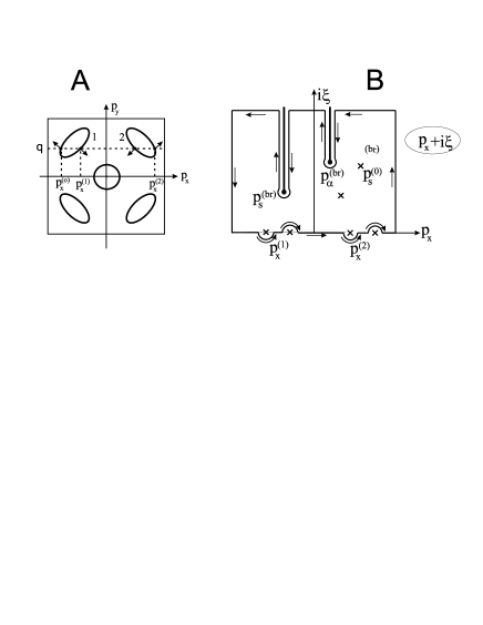
Figure 1: A. An example of the Brillouin zone with 5 contours of equal energy of energy bands $\varepsilon_{\alpha}(\mathbf{p})=\varepsilon$ with the band number $\alpha=1,2,3,4,5$. The arrows show the directions of the velocities at the points of intersections of the equal energy contours with the line of the constant $y$-projection $q$. The incident electron has the conserving momentum projection $q=p_{y}^{(in)}$ and the negative direction of the velocity $x$-projection, $v_{x}$. B. Contour of integration of Eq.(41,43). Crosses on the real axis $p_{x}$ and those in the upper complex half-plane show positions of the poles corresponding to two points with positive $v_{x}$ and to virtual states $\varepsilon_{s}(\mathbf{p})\neq\varepsilon;\;s\neq\alpha$. Thick vertical lines are brunch lines corresponding to the brunching points (thick dots) in the electron spectrum.

Below we also assume that along the edge line $x=0$ the lattice is periodic with the period $\bar{a}$ and hence the momentum projection $p_{y}$ conserves. Taking into account this requirement and using Eqs.(37,39) together with Eq.(40) and the boundary conditions for $\Psi(\mathbf{r})$ one finds the wave function on the right half-plane $x\geq 0$ as follows:

$$\Psi(\mathbf{r})=\frac{\varphi_{s_{0},\mathbf{p}_{0}}^{(in)}}{\sqrt{v_{x,s_{0}}}}+\frac{\hbar^{2}}{2m}\int_{-\infty}^{\infty}d\bar{y}\Psi_{x}^{\prime}(-0,\bar{y})$$

$$\times\sum_{s}\int dp_{x}\frac{\varphi_{s,p_{x},q}^{\star}(-0,\bar{y})\varphi_{s,p_{x},q_{y}}(\mathbf{r})}{\varepsilon-\varepsilon_{s}(p_{x},q_{y})+i\delta}$$ (41)

where $v_{x,s_{0}}<0$ is the $x$-projection of the velocity of the incident electron that normalizes its wave function to the unity flux; $q_{y}\equiv p_{0}^{y}$ is the conserving $y$-projection of the momentum $\mathbf{p}_{0}$ of the incident electron; $\Psi_{x}^{\prime}(-0,\bar{y})=\partial\Psi(\mathbf{r})/\partial x$ at $x=-0$; as the value of $\Psi$-function in Eq.(41) exactly on the boundary contour is a matter of convention (see Ref.Morse ) the boundary contour is assumed to be shifted to $x=-0\equiv 0-\bar{\delta},\;\bar{\delta}\rightarrow 0$ while $\Psi(\mathbf{r})$ is defined on the half-plane $x\geq 0$.

It is now necessary to introduce the integral equation for $\Psi_{x}^{\prime}(-0,\bar{y})$ solution of which completes the definition of the wave function $\Psi(\mathbf{r})$:

$$\Psi_{x}^{\prime}(0,y)=\frac{1}{\sqrt{v_{x,s_{0}}}}\frac{\partial\varphi_{s_{0},\mathbf{p}_{0}}^{(in)}}{\partial x}\Big{|}_{x=0}$$

$$+\frac{\hbar^{2}}{2m}\int_{-\infty}^{\infty}d\bar{y}\Psi_{x}^{\prime}(0,\bar{y})$$

$$\times\sum_{s}\int dp_{x}\frac{\varphi_{s,p_{x},q}^{\star}(0,\bar{y})\varphi^{\prime}_{s,p_{x},q_{y}}(0,y)}{\varepsilon-\varepsilon_{s}(p_{x},q)+i\delta}\hskip 5.69046pt$$ (42)

Here $f^{\prime}(\mathbf{r})=\partial f(\mathbf{r})/\partial x$.

In the general case and without usage of an approximate model this integral equation can not be solved. However, important general features (in terms of $\Psi_{x}^{\prime}(0,\bar{y})$) of the quasi-particle scattering by the abrupt lattice edge follow from Eq.(41).

Indeed, let us consider one-dimensional integrals in Eq.(41) presenting them in the form

$$I=\int_{-b_{x}/2}^{b_{x}/2}\frac{u_{s,p_{x},q_{y}}^{\star}(0,\bar{y})u_{s,p_{x},q_{y}}(\mathbf{r})e^{ixp_{x}/\hbar}}{\varepsilon-\varepsilon_{s}(p_{x},q_{y})+i\delta}dp_{x}$$ (43)

Here $b_{x}$ is the period of the reciprocal lattice in the $x$-direction. In the complex plane the dispersion law $\varepsilon_{s}(p_{x},q)$ considered as a function of the complex variable $z=p_{x}+i\xi$ is a multi-valued function which has branching points in the complex plane and hence this integral is a sum of the residues minus sum of integrals along the brunch cuts in the upper complex half-plane $\xi\geq 0$ inside the contour schematically shown in Fig.1. The left and right vertical lines of the contour are separated by the reciprocal period period $b_{x}$ and hence the integrals along them cancel each other because the integrands are periodic functions of the same period. The integral along its upper horizonal part exponentially goes to zero as this contour part goes to $i\infty$.

The poles and branching cuts of the integrand which contribute to the integral Eq.(43) are separated in two types:

1. Poles lying on the upper side of the real axis

$$p_{x}=p_{x}^{(\alpha)}+i\frac{\delta}{v_{x}^{(\alpha)}},\;\alpha=1,2,...,\;\delta\rightarrow 0$$

where their real parts $p_{x}^{(\alpha)}$ are determined by the equation

$$\varepsilon=\varepsilon_{\alpha}(p_{x},q_{y})$$ (44)

while $\alpha$ defines the number of the band which are present in the infinite lattice at the energy $\varepsilon$ and the momentum projection $p_{y}=q$ (in Fig.1 they are shown as pockets with the band numbers $\alpha=1,2$). One easily sees that these poles are inside the integration contour if the x-projections of the velocity

$$v_{x,\alpha}=\frac{\partial\varepsilon_{\alpha}(p_{x},q_{y})}{\partial p_{x}}\Big{|}_{p_{x}^{(\alpha)}}>0$$ (45)

and, therefore, they correspond to the states of electrons reflected back by the boundary.

2. Poles lying high in the upper complex plane $p_{s}^{(0)}=p_{x}^{s}+ib_{s}^{(0)}$ which are determined by the equation $\varepsilon=\varepsilon_{s}(p_{x},q_{y}),\;s\neq\alpha$ where the energy bands $\varepsilon_{s}(p_{x},q_{y})$ do not overlap bands $\alpha$ (in which the energy $\varepsilon$ lies).

As the dispersion law $\varepsilon_{s}(p_{x},q)$ is a multi-valued functions of $p_{x}$ (a circuit around the branching point changes the band number $s$) there are branching cuts in the upper half plane $z=p_{x}+i\xi$, schematically shown in Fig.1, which pass from the branching points $p_{s}^{br)}=p_{x,s}^{(br)}+i\xi_{s}^{(br)}$ to $p_{x,s}^{(br)}+i\infty$).

Taking into account the above-mentioned poles and branch cuts one easily carried out integration in Eq.(43) and, inserting the result in Eq.(41), one writes the required wave function as follows:

$$\Psi(\mathbf{r})=\frac{\varphi_{s_{0},\mathbf{p}_{0}}^{(in)}}{\sqrt{v_{x,s_{0}}}}+\sum_{\alpha}C_{\alpha}\frac{\varphi_{\alpha,p_{x}^{\alpha}}(x,y)}{\sqrt{v_{x,\alpha}}}$$

$$+\left[\sum_{s\neq\alpha}C_{s}\frac{\phi_{s,p_{s}^{(0)}}(x,y)}{\sqrt{v_{x,s}}}e^{-b_{s}^{(0)}x/\hbar}\right.\hskip 42.67912pt$$

$$+\left.\sum_{\bar{s}}\int_{\xi_{br}^{(\bar{s})}}^{\infty}B_{\bar{s}}(\zeta)\phi_{\bar{s},p_{\bar{s}}^{(br)}(\zeta)}(x,y)e^{-x\zeta/\hbar}d\zeta\right]$$ (46)

where summation $\bar{s}=s,\alpha$ (that is summation with respect to $\bar{s}$ is over all electron bands including all $\alpha$-bands), the integral is taken along the $\bar{s}$-branching cut in which the variable change $\zeta=i\xi$ has been done; the functions in square brackets are

$$\phi_{s,p_{s}^{(0)}}=u_{s,p_{s}^{(0)}}\exp\{i\frac{xp_{x}^{(s)}+qy}{\hbar}\}\hskip 34.14322pt$$

$$\phi_{\bar{s},p_{\bar{s}}^{(br)}(\zeta)}=u_{\bar{s},p_{\bar{s}}^{(br)}(\zeta)}\exp\{i\frac{xp_{x,\bar{s}}^{(br)})+qy}{\hbar}\}$$ (47)

where $p_{s}^{(br)}(\zeta)=p_{x,s}^{(br)}+\zeta$; constants $A_{s},C_{\alpha}$ and $B_{\bar{s}}(\zeta)$ are presented in Appendix, Eqs.(55,56).

IV.1 Scattering of electrons by abrupt edge in 2D electron gas.

As one sees from Eq.(46) the functions in square brackets exponentially decrease with an increase of the x-coordinate. In the general case the energy gaps between non-overlapping electron bands are of the order of the band widths $\Delta E\sim 1\div 10$eV and hence the imaginary parts of the pole and branch momenta are of the order of the $\Delta E/v_{F}$ that is $b_{s}^{(0)}\sim\xi_{br}^{(\bar{s})}\sim\hbar/a$ where $a$ is the atomic spacing.

From the above considerations and Eq.(46) it follows that inside the layer $x\lesssim a$ adjacent to the sample boundary the electron wave function is a superposition of Bloch wave functions $\varphi_{\mathbf{s}}$ of all energy bands including those virtual which are above and below the band of the incident electron (that is their band numbers $s\neq\alpha$).

At the distances much larger than the atomic spacing, $x\gg a$, all the virtual wave functions exponentially drop out from the superposition and the electro wave function $\Psi$ reduces to

$$\Psi(\mathbf{r})=\varphi_{s_{0},\mathbf{p}_{0}}^{(in)}+\sum_{\alpha}C_{\alpha}\frac{\varphi_{\alpha,p_{x}^{(\alpha)}}(x,y)}{\sqrt{v_{x,\alpha}}}+\textsl{O}(e^{-x/a})$$ (48)

According to the calculations the Bloch functions under the summation sign belong to the states with the positive x-projections of the electron velocity (see Eq.(45) Fig.1A). Therefore, they are the Bloch functions of the electron scattered back by the sample boundary into all the available energy bands at the energy of the incident electron $\varepsilon$ and the conserving $y$-projection of the momentum while constants $C_{\alpha}$ are the probability amplitudes of this many-channel scattering (an example of such the two-channel scattering is presented in in Fig.1A).

The above general scattering scenario requires a special treatment in the case of the generation when the top and the bottom of two energy bands are very close or coincide in some point of the reciprocal space as it takes place in graphene. In the next section the scattering of quasi-particles by a sharp graphene boundary is considered.

IV.2 Scattering of quasi-particles by abrupt edge of graphene sheet.

In this section scattering of quasi-particles in graphene by an abrupt edge is considered. Graphene fills the half-plane $x\geq 0$ while the boundary condition for the quasi-particle wave function is $\Psi^{(gr)}(0,y)=0$

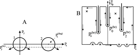
Figure 2: A. Shematic representation of two equal energy contours $v\sqrt{p_{x}^{2}+p_{y}^{2}}=\varepsilon$ and $v\sqrt{(p_{x}-p_{x}^{deg})^{2}+p_{y}^{2}}=\varepsilon$. The arrows show directions of the velocities at the points of intersections of the equal energy contours with the line of the constant $y$-projection $q$. The incident electron has the conserving momentum projection $q=p_{y}^{(in)}$ and the negative direction of the velocity $x$-projection, $v_{x}=vp_{x}/p$. B. Contour of integration of Eq.(41,43). Crosses on the real axis $p_{x}$ and those in the upper complex half-plane show positions of the poles corresponding to two points with positive $v_{x}$ and to virtual states $\varepsilon_{s}(\mathbf{p})\neq\varepsilon;\;s\neq\alpha$. Thick vertical lines are brunch lines corresponding to the brunching points (thick dots) in the quasi-psrticle spectrum.

In the general approach to the scattering problem developed above, the only peculiarity of the scattering of quasi-particles in graphene lies in their dispersion law whereas all the equations of the previous section remain valid.

The incident electron in graphene with a negative $x$-projection of the velocity in the Bloch state $\varphi_{\mathbf{p}^{(in)}}^{(gr,in)}$ and the energy $\varepsilon>0$ belonging (for the sake ofcertainty) to the electronic band $\varepsilon_{+}(p)=+vp$ is considered (see Fig.2A).

Inserting the graphene quasi-particle dispersion law Eq.(8) in Eq.(46) one finds the electron wave function at the distances much greater that the deBroglie’s wave length $x\gg\lambda_{B}=\hbar v/\varepsilon$ as follows (details of calculations are given in Appendix B):

$$x\gg\frac{\hbar v}{\varepsilon},\hskip 170.71652pt$$

$$\Psi^{(gr)}(\mathbf{r})=\frac{\varphi_{\mathbf{p}^{(in)}}^{(gr,in)}}{\sqrt{v_{x}}}+\sum_{\alpha=1,2}C_{\alpha}^{(gr)}\frac{\varphi_{\alpha,p_{x}^{\alpha},p_{y}^{(in)}}^{(gr;+)}(x,y)}{\sqrt{v_{x,\alpha}}}$$

$$+\sum_{\nu=\pm}\sum_{\alpha=1,2}B_{\alpha}^{(gr;\nu)}\varphi_{\alpha;{p_{x}}^{(gr)},p_{y}^{(in)}}^{(gr;\nu)}(x,y)\frac{e^{-xp_{y}^{(in)}/\hbar}}{x}$$ (49)

Here Bloch functions $\varphi_{\alpha,\mathbf{p}}^{(gr)}$ (see Eq.(11) are

$$\varphi_{\alpha,\mathbf{p}}^{(gr;\pm)}(\mathbf{r})=g_{\alpha}\exp{i\frac{\mathbf{pr}}{\hbar}}$$

$$\left(\begin{array}[]{cc}u_{1,\mathbf{{p}}_{\alpha}^{(gr)}}^{(\pm)}(\mathbf{r})&0\\ 0&u_{2,\mathbf{{p}}_{\alpha}^{(gr)}}^{(\pm)}(\mathbf{r})\\ \end{array}\right)\left(\begin{array}[]{c}1\\ e^{\mp i\theta}\\ \end{array}\right)$$ (54)

where $g_{\alpha}$ is the normalizing constant and $\mathbf{{p}}_{1}^{(gr)}=0$ for $\alpha=1$, while for $\alpha=2$ it is equal to the coordinate of the second cone $\mathbf{p}^{(deg)}_{2}$; note that $p_{y}^{(in)}$ is the conserving $y$-projection of the incident quasi-particle momentum.

Therefore, as it follows from Eqs.(46,49), near the graphene lattice boundary, inside the layer $x\lesssim a$ ($a$ is the atomic spacing), the quasi-particle wave function is a superposition of Bloch wave functions belonging to all energy bands (including those virtual). At the distance much larger than deBrouglie’s wave length $\lambda_{B}=\hbar v/\varepsilon$ the superposition reduces to the sum of the Bloch functions of the reflected electron, Eq.(15), (note, it was assumed that an electron was the incident quasi-particle) of the infinite graphene sample plus additional terms proportional to the graphene Bloch functions with the momentum the both projections of which are equal to the conserving $y$-projection of the incident quasi-particle $p_{y}^{(in)}$. The latter terms slowly decrease at the distances $\delta x\lesssim\hbar/|p_{y}^{(in)}|\ll\varepsilon/v$. If the normal incidence of the quasi-article on the graphene boundary takes place, $p_{y}^{(in)}=0$, these terms decease as $1/x$.

V Conclusion.

In this paper the problem of scattering of quasi-particles by an abrupt edge in the 2D electron gas and in graphene lattice is considered by the Qreen’s function technique. This approach allows to find the coordinate dependence of the wave function of the quasi-particle reflected at such an edge and the boundary conditions in a rather simple way. In particular, it is shown that the wave function of the reflected quasi-particle in graphene contains terms slowly decreasing with an increase of the distance to the edge. In the case of the transverse incidence they are inverse proportional to this distance.

For graphene the Dirac equation, the momentum dependence of the wave functions near the conic points and the dispersion law are derived by the perturbation method with degeneracy in terms of the Bloch functions the periodic factors of which are taken at the degeneracy point (the conic point). This approach allows to formulate the lattice symmetry and external field properties needed for validity of the Dirac equation in grahene and other two-dimensional conductors with degenerated energy bands.

Acknowledgement. The author thanks A.F. Volkov for useful discussions.

Appendix A

After taking thew integral in Eq.(43) and the use of Eq.(41) one finds constants $C_{\alpha},\;C_{s}$ and function $B_{\bar{s}}(\zeta)$ as follows:

$$C_{\alpha}=2\pi i\frac{\hbar^{2}}{2m}\int_{-\infty}^{\infty}d\bar{y}\Psi_{x}^{\prime}(0,\bar{y})\frac{\varphi^{\star}_{s,p_{x}^{(\alpha)}}(0,\bar{y})}{\sqrt{v_{x,\alpha}}}$$

$$C_{s}=2\pi i\frac{\hbar^{2}}{2m}\int_{-\infty}^{\infty}d\bar{y}\Psi_{x}^{\prime}(0,\bar{y})\frac{\phi^{\star}_{s,p_{s}^{(0)}}(0,\bar{y})}{\sqrt{v_{x,s}}}$$ (55)

and

$$B_{\bar{s}}(\zeta)=\frac{\hbar^{2}}{2m}\int_{-\infty}^{\infty}\frac{\Psi_{x}^{\prime}(0,\bar{y})\phi^{\star}_{\bar{s},p_{\bar{s}}^{(br)}(\zeta)}(0,\bar{y})}{\varepsilon-\varepsilon_{\bar{s}}(p_{x,s}^{(br)}+\zeta,q))+i\delta}d\bar{y}.$$ (56)

Appendix B Coordinate dependence of the integral along the cut for graphene.

Using the grapene dispersion law Eq.(8) and Eq.(56) one re-writes the terms in the last sum in Eq.(46) related to the energy bands with the grapene dispersion laws, $\alpha=1,2$, as follows:

$$\frac{\hbar^{2}}{2m}\int_{-\infty}^{\infty}d\bar{y}\Psi^{\prime}_{x}(0,\bar{y})e^{ip_{y}^{(in)}(\bar{y}-y)/\hbar}$$

$$\times u_{\alpha;\mathbf{{p}}^{(gr)}}^{(gr)\star}(0,\bar{y})u^{(gr)}_{\alpha;\mathbf{{p}}^{(gr)}}(\mathbf{r})J_{\alpha}^{(gr)}(\bar{y},\mathbf{r})$$ (57)

where

$$J_{\alpha}^{(gr)}=\int_{q}^{\infty}\frac{e^{-x\zeta/\hbar}}{\varepsilon\mp v\sqrt{-\zeta^{2}+q^{2}}+i\delta}d\zeta$$ (58)

Changing the variables $\zeta-q\rightarrow\zeta$ one gets

$$J_{\alpha}^{(gr)}=e^{-qx/\hbar}\int_{0}^{\infty}\frac{e^{-x\zeta/\hbar}}{\varepsilon\mp iv\sqrt{\zeta(\zeta+2q}}d\zeta$$ (59)

As one sees from Eq.(59) the main contribution of the integrand to the integral is at $\zeta\lesssim\hbar/x$. This inequality means that the square root in the integral denominator is much less than $\varepsilon/v$ (note that $|p_{y}^{(in)}\ \lesssim\varepsilon/v$). Therefore, neglecting the term with the square root one easily takes the integral and obtains the result presented in Eq.(49) of the main text in which constants $B_{\alpha}$ are

$$B_{\alpha}^{(gr;\pm)}=$$

$$\frac{\hbar^{2}}{2m}\int_{-\infty}^{\infty}d\bar{y}\Psi^{\prime}_{x}(0,\bar{y})\varphi_{\alpha;p_{y}^{(gr)},p_{y}^{(in)}}^{(gr;\pm)}(0,\bar{y})d\bar{y}$$ (60)

References

- (1) Th. Heinzel Mesoscopic, Electronics in Solid State Nanos- tructurs (Wiley, New York, 2003).
- (2) Th. Dittrich, P. Hänggi, G.-L. Ingold, B. Kramer, G. Schön, W. Zwerger, Quantum Tranasport and Dissipation (Wiley, New York, 1998).
- (3) P.R. Wallace, Phys. Rev. 71, 622 (1947).
- (4) D.P. DiVincenzo and E.J. Mele, Phys. Rev. B 29, 1685 (1984).
- (5) Y.-W. Son, M.L. Cohen, and S.G.Louie, Phys. Rev. Lett. 97, 216803 (2006).
- (6) A. H. Castro Neto, F. Guinea, N. M. R. Peres, K. S. Novoselov, and A. K. Geim, Rev. Mod. Phys. 81, 109 (2009).
- (7) S. Das Sarma, Shaffique Adam, E.H. Hwang and Enrico Rossi, Rev. Mod. Phys. 83, 109 (2011).
- (8) E. McCann and V.I. Fal’ko, J. Phys.: Condence.Matter 16, 2371 (2004).
- (9) A.R. Akhmerov and C.W.J. Beenakker, Phys. Rev.B, 77, 085423 (2008).
- (10) L.D. Landau and E.M. Lifshitz, Qauntum Mechanics, § 79, The intersection of electron terms, (Oxford: Butterworth-Heinemann) 1998.
- (11) A.A. Slutskin, Zh. Eksp. Teor. Fiz. 53, 767 (1967) [Sov. Phys. - JETP, 26, 474 (1968)].
- (12) C.W.J. Beenakker, Rev. Mod. Phys., 80, 1337 (2008).
- (13) L.D. Landau and E.M. Lifshitz, Qauntum Mechanics, § 90, Pre-dissociaion, (Oxford: Butterworth-Heinemann) 1998;
- (14) E.I. Blount, Phys. Rev. , 126, 1636 (1962).
- (15) A.A. Slutskin and A.M. Kadigrobov, Fiz. Tverd. Tela (Leningrad) 9, 184 (1967) [Sov. Phys. - Solid State 9, 138 (1967)].
- (16) P.M. Morse and H. Feshbach, Methods of Theoretical Physics, Part I, §7.2, 805, McGraw-Hill Book Company, New York, Toronto, London (1953).