Privacy-preserving Stacking with Application to
Cross-organizational Diabetes Prediction

Abstract

To meet the standard of differential privacy, noise is usually added into the original data, which inevitably deteriorates the predicting performance of subsequent learning algorithms. In this paper, motivated by the success of improving predicting performance by ensemble learning, we propose to enhance privacy-preserving logistic regression by stacking. We show that this can be done either by sample-based or feature-based partitioning. However, we prove that when privacy-budgets are the same, feature-based partitioning requires fewer samples than sample-based one, and thus likely has better empirical performance. As transfer learning is difficult to be integrated with a differential privacy guarantee, we further combine the proposed method with hypothesis transfer learning to address the problem of learning across different organizations. Finally, we not only demonstrate the effectiveness of our method on two benchmark data sets, i.e., MNIST and NEWS20, but also apply it into a real application of cross-organizational diabetes prediction from RUIJIN data set, where privacy is of a significant concern.

1 Introduction

In recent years, data privacy has become a serious concern in both academia and industry Dwork et al. (2006); Chaudhuri et al. (2011); Dwork and Roth (2014); Abadi et al. (2016). There are now privacy laws, such as Europe’s General Data Protection Regulation (GDPR), which regulates the protection of private data and restricts data transmission between organizations. These raise challenges for cross-organizational machine learning Pathak et al. (2010); Hamm et al. (2016); Papernot et al. (2017); Xie et al. (2017), in which data have to be distributed to different organizations, and the learning model needs to make predictions in private.

A number of approaches have been proposed to ensure privacy protection. In machine learning, differential privacy Dwork and Roth (2014) is often used to allow data be exchanged among organizations. To design a differentially private algorithm, carefully designed noise is usually added to the original data to disambiguate the algorithms. Many standard learning algorithms have been extended for differential privacy. These include logistic regression Chaudhuri et al. (2011), trees Emekçi et al. (2007); Fong and Weber-Jahnke (2012), and deep networks Shokri and Shmatikov (2015); Abadi et al. (2016). In particular, linear models are simple and easy to understand, and their differentially private variants (such as privacy-preserving logistic regression (PLR)) Chaudhuri et al. (2011)) have rigorous theoretical guarantees Chaudhuri et al. (2011); Bassily et al. (2014); Hamm et al. (2016); Kasiviswanathan and Jin (2016). However, the injection of noise often degrades prediction performance.

Ensemble learning can often signficantly improve the performance of a single learning model Zhou (2012). Popular examples include bagging Breiman (1996a), boosting Friedman et al. (2000), and stacking Wolpert (1992). These motivate us to develop an ensemble-based method which can benefit from data protection, while enjoying good prediction performance. Bagging and boosting are based on partitioning of training samples, and use pre-defined rules (majority or weighted voting) to combine predictions from models trained on different partitions. Bagging improves learning performance by reducing the variance. Boosting, on the other hand, is useful in converting weak models to a strong one. However, the logistic regression model, which is the focus in this paper, often has good performance in many applications, and is a relatively strong classifier. Besides, it is a convex model and relatively stable.

Thus, in this paper, we focus on stacking. While stacking also partitions the training data, this can be based on either samples Breiman (1996b); Smyth and Wolpert (1999); Ozay and Vural (2012) or features Boyd et al. (2011). Multiple low-level models are then learned on the different data partitions, and a high-level model (typically, a logistic regression model) is used to combine their predictions. By combining with PLR, we show how differential privacy can be ensured in stacking. Besides, when the importance of features is known a priori, they can be easily incorporated in feature-based partitioning. We further analyze the learning guarantee of sample-based and feature-based stacking, and show theoretically that feature-based partitioning can have lower sample complexity (than sample-based partitioning), and thus better performance. By adapting the feature importance, its learning performance can be further boosted.

To demonstrate the superiority of the proposed method, we perform experiments on two benchmark data sets (MNIST and NEWS20). Empirical results confirm that feature-based stacking performs better than sample-based stacking. It is also better than directly using PLR on the training data set. Besides, the prediction performance is further boosted when feature importance is used. Finally, we apply the proposed approach for cross-organizational diabetes prediction in the transfer learning setting. The experiment is performed on the RUIJIN data set, which contains over ten thousands diabetes records from across China. Results show significantly improved diabetes prediction performance over the state-of-the-art, while still protecting data privacy.

Notation. In the sequel, vectors are denoted by lowercase boldface, and $(\cdot)^{\top}$ denotes transpose of a vector/matrix; $\sigma(a)=\nicefrac{{\exp(a)}}{{(1+\exp(a))}}$ is the sigmoid function. A function $g$ is $\mu$-strongly convex if $g(\alpha{\bm{\mathbf{w}}}+(1-\alpha){\bm{\mathbf{u}}})\leq\alpha g({\bm{\mathbf{w}}})+(1-\alpha)g({\bm{\mathbf{u}}})-\frac{\mu}{2}\alpha(1-\alpha)\|{\bm{\mathbf{w}}}-{\bm{\mathbf{u}}}\|^{2}$ for any $\alpha\in(0,1)$.

2 Related Works

2.1 Differential Privacy

Differential privacy Dwork et al. (2006); Dwork and Roth (2014) has been established as a rigorous standard to guarantee privacy for algorithms that access private data. Intuitively, given a privacy budget $\epsilon$, an algorithm preserves $\epsilon$-differentially privacy if changing one entry in the data set does not change the likelihood of any of the algorithm’s output by more than $\epsilon$. Formally, it is defined as follows.

Definition 1 (Dwork et al. (2006)).

A randomized mechanism $M$ is $\epsilon$-differentially private if for all output $t$ of $M$ and for all input data $\mathcal{D}_{1},\mathcal{D}_{2}$ differing by one element, $\text{Pr}(M(\mathcal{D}_{1})=t)\leq e^{\epsilon}\,\text{Pr}(M(\mathcal{D}_{2})=t)$.

To meet the $\epsilon$-differentially privacy guarantee, careful perturbation or noise usually needs to be added to the learning algorithm. A smaller $\epsilon$ provides stricter privacy guarantee but at the expense of heavier noise, leading to larger performance deterioration Chaudhuri et al. (2011); Bassily et al. (2014). A relaxed version of $\epsilon$-differentially private, called $(\epsilon,\delta)$-differentially privacy in which $\delta$ measures the loss in privacy, is proposed Dwork and Roth (2014). However, we focus on the more stringent Definition 1 in this paper.

2.2 Privacy-preserving Logistic Regression (PLR)

Logistic regression has been popularly used in machine learning Friedman et al. (2012). Various differential privacy approaches have been developed for logistic regression. Examples include output perturbation Dwork et al. (2006); Chaudhuri et al. (2011), gradient perturbation Abadi et al. (2016) and objective perturbation Chaudhuri et al. (2011); Bassily et al. (2014). In particular, objective perturbation, which adds designed and random noise to the learning objective, has both privacy and learning guarantees as well as good empirical performance.

Privacy-preserving logistic regression (PLR) Chaudhuri et al. (2011) is the state-of-the-art model based on objective perturbation. Given a data set $\mathcal{D}=\{{\bm{\mathbf{x}}}_{i}$, $y_{i}\}_{i=1}^{n}$, where ${\bm{\mathbf{x}}}_{i}\in{\mathbb{R}}^{d}$ is the sample and $y_{i}$ the corresponding class label, we first consider the regularized risk minimization problem:

$$\min_{{\bm{\mathbf{w}}}}\nicefrac{{1}}{{n}}\sum\nolimits_{i=1}^{n}\ell({\bm{\mathbf{w}}}^{\top}{\bm{\mathbf{x}}}_{i},y_{i})+\lambda g({\bm{\mathbf{w}}}),$$ (1)

where ${\bm{\mathbf{w}}}$ is a vector of the model parameter, $\ell(\hat{y},y)=\log(1+e^{-y\hat{y}})$ is the logistic loss (with predicted label $\hat{y}$ and given label $y$), $g$ is the regularizer and $\lambda\geq 0$ is a hyperparameter. To guarantee privacy, Chaudhuri et al. (2011) added two extra terms to (1), leading to:

$$\min_{{\bm{\mathbf{w}}}}\nicefrac{{1}}{{n}}\sum\nolimits_{i=1}^{n}\ell({\bm{\mathbf{w}}}^{\top}{\bm{\mathbf{x}}}_{i},y_{i})\!+\!\nicefrac{{{\bm{\mathbf{b}}}^{\top}\!{\bm{\mathbf{w}}}}}{{n}}\!+\!\nicefrac{{\Delta\|{\bm{\mathbf{w}}}\|^{2}}}{{2}}+\lambda g({\bm{\mathbf{w}}}),$$ (2)

where ${\bm{\mathbf{b}}}$ is random noise drawn from $h({\bm{\mathbf{b}}})\propto\exp(\nicefrac{{\epsilon^{\prime}}}{{2}}\|{\bm{\mathbf{b}}}\|)$ with $\mathbb{E}(\|{\bm{\mathbf{b}}}\|)=\nicefrac{{2d}}{{\epsilon^{\prime}}}$, $\epsilon^{\prime}$ is a privacy budget modified from $\epsilon$, and $\Delta$ is a scalar depending on $\lambda$, $n,\epsilon$. The whole PLR procedure is shown in Algorithm 1.

Algorithm 1 PLR: Privacy-preserving logistic regression.

0:  privacy budget $\epsilon$, data set $\mathcal{D}$;

1:  $\epsilon^{\prime}=\epsilon-\log(1+\nicefrac{{1}}{{2n\lambda}}+\nicefrac{{1}}{{16n^{2}\lambda^{2}}})$;

2:  if $\epsilon^{\prime}>0$ then

3:     $\Delta=0$;

4:  else

5:     $\Delta=(4n(\exp(\nicefrac{{\epsilon}}{{4}})-1))^{-1}-\lambda$ and $\epsilon^{\prime}=\nicefrac{{\epsilon}}{{2}}$;

6:  end if

7:  scale $\|{\bm{\mathbf{x}}}\|\leq 1$ for all ${\bm{\mathbf{x}}}\in\mathcal{D}$;

8:  pick a random vector ${\bm{\mathbf{b}}}$ from $h({\bm{\mathbf{b}}})\propto\exp{(\nicefrac{{\epsilon^{\prime}\|{\bm{\mathbf{b}}}\|}}{{2}})}$;

9:  obtain ${\bm{\mathbf{w}}}$ by solving (2);

10:  return  ${\bm{\mathbf{w}}}$.

Proposition 1 (Chaudhuri et al. (2011)).

If the regularizer $g$ is strongly convex, Algorithm 1 provides $\epsilon$-differential privacy.

While privacy guarantee is desirable, the resultant privacy-preserving machine learning model may not have good learning performance. In practice, the performance typically degrades dramatically because of the introduction of noise Chaudhuri et al. (2011); Rajkumar and Agarwal (2012); Bassily et al. (2014); Shokri and Shmatikov (2015). Assume that samples from $\mathcal{D}$ are drawn i.i.d. from an underlying distribution $P$. Let $L({\bm{\mathbf{w}}};P)=\mathbb{E}_{({\bm{\mathbf{x}}},y)\sim P}[\ell({\bm{\mathbf{w}}}^{\top}{\bm{\mathbf{x}}},y)]$ be the expected loss of the model. The following Proposition shows the number of samples needed for PLR to have comparable performance as a given baseline model. This bound is tight for any $\epsilon$-differential privacy algorithm, and cannot be further improved Kifer et al. (2012); Bassily et al. (2014). However, in contrast, the standard logistic regression model in (1) only needs $n>\nicefrac{{C_{1}\|\mathbf{v}\|^{2}\log(\frac{1}{\delta})}}{{\epsilon_{g}^{2}}}$ samples Shalev-Shwartz and Srebro (2008), and thus may be smaller.

Proposition 2 (Chaudhuri et al. (2011)).

Let $g(\cdot)=\nicefrac{{1}}{{2}}\|\cdot\|^{2}$, and $\mathbf{v}$ be a reference model parameter. Given $\delta>0$ and $\epsilon_{g}>0$, there exists a constant $C_{1}$ such that when

$$n\!>\!C_{1}\max\left(\nicefrac{{\|\mathbf{v}\|^{2}\log(\frac{1}{\delta})}}{{\epsilon_{g}^{2}}},\nicefrac{{d\log(\frac{d}{\delta})\|\mathbf{v}\|}}{{\epsilon_{g}\epsilon}},\nicefrac{{\|\mathbf{v}\|^{2}}}{{\epsilon_{g}\epsilon}}\right),\!\!$$ (3)

${\bm{\mathbf{w}}}$ from Algorithm 1 meets $\text{Pr}[L({\bm{\mathbf{w}}},\!P)\!\leq\!L(\mathbf{v},\!P)\!+\!\epsilon_{g}]\!\geq\!1\!-\!\delta$.

2.3 Multi-Party Data Learning

Ensemble learning has been considered with differential privacy under multi-party data learning (MPL). The task is to combine predictors from multiple parties with privacy Pathak et al. (2010). Pathak et al. [2010] first proposed a specially designed protocol to privately combine multiple predictions. The performance is later surpassed by Hamm et al. (2016); Papernot et al. (2017), which uses another classifier built on auxiliary unlabeled data. However, all these combination methods rely on extra, privacy-insensitive public data, which may not be always available. Moreover, the aggregated prediction may not be better than the best single party’s prediction.

There are also MPL methods that do not use ensemble learning. Rajkumar and Agarwal [2012] used stochastic gradient descent, and Xie et al. [2017] proposed a multi-task learning method. While these improve the performance of the previous ones based on aggregation, they gradually lose the privacy guarantee after more and more iterations.

3 Privacy-preserving Ensemble

In this section, we propose to improve the learning guarantee of PLR by ensemble learning Zhou (2012). Popular examples include bagging Breiman (1996a), boosting Friedman et al. (2000), and stacking Wolpert (1992). Bagging and boosting are based on partitioning of training samples, and use pre-defined rules (majority or weighted voting) to combine predictions from models trained on different partitions. Bagging improves learning performance by reducing the variance. However, logistic regression is a convex model and relatively stable. Boosting, on the other hand, is useful in combining weak models to a strong one, while logistic regression is a relatively strong classifier and often has good performance in many applications.

In this paper, we focus on stacking and show that its privacy-preserving version can be realized based on sample partitioning (Section 3.1) and feature partitioning (FP) (Section 3.2). However, sample partitioning (SP) may suffer from insufficient training samples, while FP does not. Besides, FP allows the incorporation of feature importance to improve learning performance.

3.1 Privacy-preserving Stacking with Sample Partitioning (SP)

We first consider using stacking with SP, and PLR is used as both the low-level and high-level models (Algorithm 2). As stacking does not impose restriction on the usage of classifiers on each partition of the training data, a simple combination of stacking and PLR can be used to provide privacy guarantee.

Algorithm 2 PST-S: Privacy-preserving stacking with SP.

0:  privacy budget $\epsilon$, data set $\mathcal{D}$;

1:  partition $\mathcal{D}$ into disjoint sets $\mathcal{D}^{l}$ and $\mathcal{D}^{h}$, for training of the low-level and high-level models, respectively;

2:  partition samples in $\mathcal{D}^{l}$ to $K$ disjoint sets $\{\mathcal{S}_{1}$, $\dots$, $\mathcal{S}_{K}\}$;

3:  for $k=1,\dots,K$ do

4:     train PLR (Algorithm 1) with privacy budget $\epsilon$ on $\mathcal{S}_{k}$, and obtain the low-level model parameter ${\bm{\mathbf{w}}}_{k}^{l}$;

5:  end for

6:  construct meta-data set $\mathcal{M}^{s}=\{[\sigma(\mathbf{x}^{\top}{\bm{\mathbf{w}}}_{1}^{l})$;$\dots$;$\sigma(\mathbf{x}^{\top}{\bm{\mathbf{w}}}_{K}^{l})],y\}$ using all samples $\{{\bm{\mathbf{x}}},y\}\in\mathcal{D}^{h}$;

7:  train PLR (Algorithm 1) with privacy budget $\epsilon$ on $\mathcal{M}^{s}$, and obtain the high-level model parameter ${\bm{\mathbf{w}}}^{h}$;

8:  return  $\{{\bm{\mathbf{w}}}_{k}^{l}\}$ and ${\bm{\mathbf{w}}}^{h}$.

Proposition 3.

If the regularizer $g$ is strongly convex, Algorithm 2 provides $\epsilon$-differential privacy.

However, while the high-level model can be better than any of the single low-level models Džeroski and Ženko (2004), Algorithm 2 may not perform better than directly using PLR on the whole $\mathcal{D}$ for the following two reasons. First, each low-level model uses only $\mathcal{S}_{k}$ (step 4), which is about $\nicefrac{{1}}{{K}}$ the size of $\mathcal{D}$ (assuming that the data set $\mathcal{D}$ is partitioned uniformly). This smaller sample size may not satisfy condition (3) in Proposition 2. Second, in many real-world applications, features are not of equal importance. For example, for diabetes prediction using the RUIJIN data set (Table 3), Glu120 and Glu0, which directly measure glucose levels in the blood, are more relevant than features such as age and number of children. However, during training of the low-level models, Algorithm 2 adds equal amounts of noise to all features. If we can add less noise to the more important features while keeping the same privacy guarantee, we are likely to get better learning performance.

3.2 Privacy-preserving Stacking with Feature Partitioning (FP)

To address the above problems, we propose to partition the data based on features instead of samples in training the low-level models. The proposed feature-based stacking approach is shown in Algorithm 3. Features are partitioned into $K$ subsets, and $\mathcal{D}^{l}$ is split correspondingly into $K$ disjoint sets $\{\mathcal{F}_{1},\dots,\mathcal{F}_{K}\}$. Obviously, as the number of training samples is not reduced, the sample size condition for learning performance guarantee is easier to be satisfied (details will be established in Theorem 4).

Algorithm 3 PST-F: Privacy-preserving stacking with FP.

0:  privacy budget $\epsilon$, data set $\mathcal{D}$, feature importance $\{q_{k}\}_{k=1}^{K}$ where $q_{k}\geq 0$ and $\sum_{k=1}^{K}{q_{k}}=1$;

1:  partition $\mathcal{D}$ into disjoint sets $\mathcal{D}^{l}$ and $\mathcal{D}^{h}$, for training of the low-level model and high-level model, respectively;

2:  partition $\mathcal{D}^{l}$ to $K$ disjoint sets $\{\mathcal{F}_{1}$, $\dots$, $\mathcal{F}_{K}\}$ based on features;

3:  $\epsilon^{\prime}=\epsilon-\sum_{k=1}^{K}\log(1+\nicefrac{{q_{k}^{2}}}{{2n\lambda_{k}}}+\nicefrac{{q_{k}^{4}}}{{16n^{2}\lambda_{k}^{2}}})$;

4:  for $k=1,\dots,K$ do

5:     scale $\|{\bm{\mathbf{x}}}\|\leq q_{k}$ for all ${\bm{\mathbf{x}}}\in\mathcal{F}_{k}$;

6:     if $\epsilon^{\prime}>0$ then

7:        $\Delta_{k}=0$ and $\epsilon_{k}=\epsilon^{\prime}$;

8:     else

9:        $\Delta_{k}=\nicefrac{{q_{k}^{2}}}{{4n(\exp(\nicefrac{{\epsilon q_{k}}}{{4}})-1)}}-\lambda_{k}$ and $\epsilon_{k}=\nicefrac{{\epsilon}}{{2}}$;

10:     end if

11:     pick a random ${\bm{\mathbf{b}}}_{k}$ from $h({\bm{\mathbf{b}}})\propto\exp(\nicefrac{{\epsilon_{k}\|{\bm{\mathbf{b}}}\|}}{{2}})$;

12:     ${\bm{\mathbf{w}}}_{k}^{l}=\arg\min_{{\bm{\mathbf{w}}}}\!\nicefrac{{1}}{{n}}\sum_{{\bm{\mathbf{x}}}_{i}\in\mathcal{F}_{k}}\ell({\bm{\mathbf{w}}}^{\top}{\bm{\mathbf{x}}}_{i},y_{i})+\nicefrac{{{\bm{\mathbf{b}}}_{k}^{\top}{\bm{\mathbf{w}}}}}{{n}}+\nicefrac{{\Delta\|{\bm{\mathbf{w}}}\|^{2}}}{{2}}+\lambda_{k}g_{k}({\bm{\mathbf{w}}})$;

13:  end for

14:  construct meta-data set $\mathcal{M}^{f}=$ $\{[\sigma({\bm{\mathbf{x}}}_{(1)}^{\top}{\bm{\mathbf{w}}}_{1}^{l})$,$\dots$,$\sigma({\bm{\mathbf{x}}}_{(K)}^{\top}{\bm{\mathbf{w}}}_{K}^{l})]$, $y\}$ using all $\{{\bm{\mathbf{x}}},y\}\in\mathcal{D}^{h}$, where ${\bm{\mathbf{x}}}_{(k)}$ is a vector made from ${\bm{\mathbf{x}}}$ by taking features covered by $\mathcal{F}_{k}$;

15:  train PLR (Algorithm 1) with privacy budget $\epsilon$ on $\mathcal{M}^{f}$, and obtain the high-level model parameter ${\bm{\mathbf{w}}}^{h}$;

16:  return  $\{{\bm{\mathbf{w}}}_{k}^{l}\}$ and ${\bm{\mathbf{w}}}^{h}$.

When the relative importance of feature subsets is known, Algorithm 3 adds less noise to the more important features. Specifically, let the importance of $\mathcal{F}_{k}$ (with $d_{k}$ features) be $q_{k}$, where $q_{k}\geq 0$ and $\sum_{k=1}q_{k}=1$, and is independent with $\mathcal{D}$. Assume that $\epsilon^{\prime}>0$ in step 6 (and thus $\epsilon_{k}=\epsilon^{\prime}$). Recall from Section 2.2 that $\mathbb{E}(\|{\bm{\mathbf{b}}}_{k}\|)=\nicefrac{{2d_{k}}}{{\epsilon_{k}}}=\nicefrac{{2d_{k}}}{{\epsilon^{\prime}}}$. By scaling the samples in each $\mathcal{F}_{k}$ as in step 5, the injected noise level in $\mathcal{F}_{k}$ is given by $\nicefrac{{\mathbb{E}(\|{\bm{\mathbf{b}}}_{k}\|)}}{{\|{\bm{\mathbf{x}}}\|}}=\nicefrac{{2d_{k}}}{{\epsilon^{\prime}q_{k}}}$. This is thus inversely proportional to the importance $q_{k}$.

Remark 1.

In the special case where only one feature group has nonzero importance, Algorithm 3 reduces Algorithm 1 on that group, and privacy is still guaranteed.

Finally, a privacy-preserving low-level logistic regression model is obtained in step 12, and a privacy-preserving high-level logistic regression model is obtained in step 15. In general, each low-level model can have its own regularizer $g_{k}$ (an example is shown in Theorem 5).

1). Privacy Guarantee. Theorem 4 guarantees privacy of Algorithm 3. Note that the proofs in Chaudhuri et al. (2011); Bassily et al. (2014) cannot be directly used, as they consider neither stacking nor feature importance.

Theorem 4.

If all $g_{k}$’s are strongly convex, Algorithm 3 provides $\epsilon$-differential privacy.

2). Learning Performance Guarantee. Analogous to Proposition 1, the following bounds the learning performance of each low-level model.

Theorem 5.

$g_{k}=\nicefrac{{1}}{{2}}\|\cdot-\mathbf{u}_{k}\|^{2}$, where $\mathbf{u}_{k}$ is any constant vector, and $\mathbf{v}_{k}$ is a reference model parameter. Let $a_{k}=q_{k}\|\mathbf{v}_{k}\|$. given $\delta>0$ and $\epsilon_{g}>0$, there exists a constant $C_{1}$ such that when

$$n\!>\!C_{1}\max\left(\nicefrac{{a_{k}^{2}\log(\nicefrac{{1}}{{\delta}})}}{{\epsilon_{g}^{2}}},\nicefrac{{d\log(\nicefrac{{d}}{{K\delta}})a_{k}}}{{q_{k}K\epsilon_{g}\epsilon}},\nicefrac{{a_{k}^{2}}}{{\epsilon_{g}\epsilon}}\right),$$ (4)

${\bm{\mathbf{w}}}_{k}^{l}$ from Algorithm 3 satisfies $\text{Pr}[L({\bm{\mathbf{w}}}_{k}^{l},P)\leq L(\mathbf{v}_{k},P)+\epsilon_{g}]\geq 1-\delta$.

Remark 2.

When $K\!=\!1$ (a single low-level model trained with all features) and $\mathbf{u}_{k}\!=\!\mathbf{0}$, Theorem 5 reduces to Proposition 2.

Note that, to keep the same bound $L({\bm{\mathbf{v}}}_{k},P)+\epsilon_{g}$, since ${\bm{\mathbf{x}}}$s’ are scaled by $q_{k}$, ${\bm{\mathbf{v}}}_{k}$ should be scaled by $\nicefrac{{1}}{{q_{k}}}$, so $\mathbb{E}(a_{k})=\mathbb{E}(q_{k}\|\mathbf{v}_{k}\|)$ remains the same as $q_{k}$ changes. Thus, Theorem 5 shows that low-level models on more important features can indeed learn better, if these features are assigned with larger $q_{k}$. Since stacking can have better performance than any single model Ting and Witten (1999); Džeroski and Ženko (2004) and Theorem 5 can offer better learning guarantee than Proposition 2, Algorithm 3 can have better performance than Algorithm 1. Finally, compared with Proposition 1, $g_{k}$ in theorem 5 is more flexible in allowing an extra $\mathbf{u}_{k}$. We will show in Section 3.3 that this is useful for transfer learning.

Since the learning performance of stacking itself is still an open issue Ting and Witten (1999), we leave the guarantee for the whole Algorithm 3 as future work. A potential problem with FP is that possible correlations among feature subsets can no longer be utilized. However, as the high-level model can combine information from various low-level models, empirical results in Section 4.1 show that this is not problematic unless $K$ is very large.

3.3 Application to Transfer Learning

Transfer learning Pan and Yang (2010) is a powerful and promising method to extract useful knowledge from a source domain to a target domain. A popular transfer learning approach is hypothesis transfer learning (HTL) Kuzborskij and Orabona (2013), which encourages the hypothesis learned in the target domain to be similar with that in the source domain. For application to (1), HTL adds an extra regularizer as:

$$\min_{{\bm{\mathbf{w}}}}\sum\nolimits_{{\bm{\mathbf{x}}}_{i}\in\mathcal{D}_{\text{tgt}}}\ell({\bm{\mathbf{w}}}^{\top}{\bm{\mathbf{x}}}_{i},y_{i})\!+\!\lambda g({\bm{\mathbf{w}}})\!+\!\nicefrac{{\eta}}{{2}}\|{\bm{\mathbf{w}}}\!-\!{\bm{\mathbf{w}}}_{\text{src}}\|^{2}.$$ (5)

Here, $\eta$ is a hyperparameter, $\mathcal{D}_{\text{tgt}}$ is the target domain data, and ${\bm{\mathbf{w}}}_{\text{src}}$ is obtained from the source domain. Algorithm 4 shows how PST-F can be extended with HTL using privacy budgets $\epsilon_{\text{src}}$ and $\epsilon_{\text{tgt}}$ for the source and target domains, respectively. The same feature partitioning is used on both the source and target data. PLR is trained on each source domain data subset to obtain $({\bm{\mathbf{w}}}_{\text{src}})_{k}$ (steps 2-4). This is then transferred to the target domain using PST-F with $g_{k}({\bm{\mathbf{w}}})\!=\!\frac{1}{2}\|{\bm{\mathbf{w}}}\!-\!({\bm{\mathbf{w}}}_{\text{src}})_{k}\|^{2}$ (step 5).

Algorithm 4 PST-H: Privacy-preserving stacking with HTL.

0:  source data sets $\mathcal{D}_{\text{src}}$, target data set $\mathcal{D}_{\text{tgt}}$, and corresponding privacy budgets $\epsilon_{\text{src}}$ and $\epsilon_{\text{tgt}}$, respectively. (source domain processing)

1:  partition $\mathcal{D}_{\text{src}}$ to $K$ disjoint sets $\left\{\mathcal{F}_{1},\dots,\mathcal{F}_{K}\right\}$ based on features;

2:  for $k=1,\dots,K$ do

3:     train PLR with privacy budget $\epsilon_{\text{src}}$ on $\mathcal{F}_{k}$ and obtain $({\bm{\mathbf{w}}}_{\text{src}})_{k}$;

4:  end for(target domain processing)

5:  obtain $\left\{({\bm{\mathbf{w}}}_{\text{tgt}})_{k}^{l}\right\}$ and ${\bm{\mathbf{w}}}_{\text{tgt}}^{h}$ from PST-F (Algorithm 3) by taking $g_{k}({\bm{\mathbf{w}}})\!=\!\nicefrac{{1}}{{2}}\|{\bm{\mathbf{w}}}\!-\!({\bm{\mathbf{w}}}_{\text{src}})_{k}\|^{2}$ and privacy budget $\epsilon_{\text{tgt}}$ on $\mathcal{D}_{\text{tgt}}$;

6:  return  $\left\{({\bm{\mathbf{w}}}_{\text{src}})_{k}\right\}$ for source domain, $\left\{({\bm{\mathbf{w}}}_{\text{tgt}})_{k}^{l}\right\}$ and ${\bm{\mathbf{w}}}_{\text{tgt}}^{h}$ for target domain.

The following provides privacy guarantees on both the source and target domains.

Corollary 6.

Algorithm 4 provides $\epsilon_{\text{src}}$- and $\epsilon_{\text{tgt}}$-differential privacy guarantees for the source and target domains.

Recently, privacy-preserving HTL is also proposed in Wang et al. (2018). However, it does not consider stacking and ignores feature importance.

4 Experiments

Experiments are performed on a server with Intel Xeon E5 CPU and 250G memory. All codes are in Python.

4.1 Benchmark Datasets

Experiments are performed on two popular benchmark data sets for evaluating privacy-preserving learning algorithms Shokri and Shmatikov (2015); Papernot et al. (2017); Wang et al. (2018): MNIST LeCun et al. (1998) and NEWS20 Lang (1995) (Table 1). The MNIST data set contains images of handwritten digits. Here, we use the digits $0$ and $8$. We randomly select 5000 samples. $60\%$ of them are used for training (with $\nicefrac{{1}}{{3}}$ of this used for validation), and the remaining $20\%$ for testing. The NEWS20 data set is a collection of newsgroup documents. Documents belonging to the topic “sci” are taken as positive samples, while those in the topic “talk” are taken as negative. Finally, we use PCA to reduce the feature dimensionality to $100$, as original dimensionality for MINIST/NEWS20 is too high for differentially private algorithms to handle as the noise will be extremely large.

MNIST			NEWS20
#train	#test	#features	#train	#test	#features
3000	2000	100	4321	643	100

Table 1: Summary of the MNIST and NEWS20 data sets.

The following algorithms are compared: (i) PLR, which applies Algorithm 1 on the training data; (ii) PST-S: Algorithm 2, based on SP; and (iii) PST-F: Algorithm 3, based on FP. We use $K=5$ and $50\%$ of the data for $\mathcal{D}^{l}$ and the remaining for $\mathcal{D}^{h}$. Two PST-F variants are compared: PST-F(U), with random FP and equal feature importance. And PST-F(W), with partitioning based on the PCA feature scores; and the importance of the $k$th group $\mathcal{F}_{k}$ is

$$q_{k}=\nicefrac{{\sum\nolimits_{i:f_{i}\in\mathcal{F}_{k}}v_{i}}}{{\sum\nolimits_{j:f_{j}\in\mathcal{D}^{l}}v_{j}}},$$ (6)

where $v_{i}$ is the variance of the $i$th feature $f_{i}$. Gradient perturbation is worse than objective perturbation in logistic regression Bassily et al. (2014), thus is not compared.

The area-under-the-ROC-curve (AUC) Hanley and McNeil (1983) on the testing set is used for performance evaluation. Hyper-parameters are tuned using the validation set. To reduce statistical variations, the experiment is repeated $10$ times, and the results averaged.

1). Varying Privacy Budget $\epsilon$. Figure 1 shows the testing AUC’s when the privacy budget $\epsilon$ is varied. As can be seen, the AUCs for all methods improve when the privacy requirement is relaxed ($\epsilon$ is large and less noise is added). Moreover, PST-S can be inferior to PLR, due to insufficient training samples caused by SP. Both PST-F(W) and PST-F(U) have better AUCs than PST-S and PLR. In particular, PST-F(W) is the best as it can utilize feature importance. Since PST-S is inferior to PST-F(U), we only consider PST-F(U) in the following experiments.

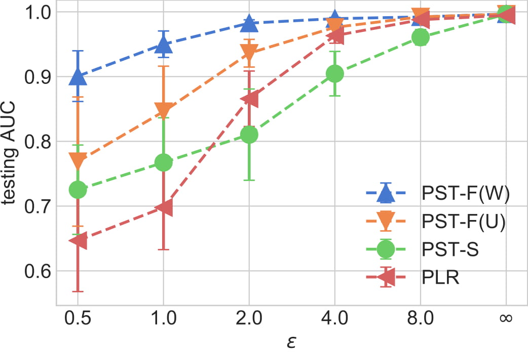
(a) MNIST.

(b) NEWS20.

Figure 1: Testing AUC vs $\epsilon$. Here, “$\infty$” corresponds to the non-privacy-preserving version of the corresponding algorithms.

2). Varying Number of Partitions $K$. In this experiment, we fix $\epsilon=1$, and vary $K$. As can be seen from Figure 2, when $K$ is very small, ensemble learning is not effective. When $K$ is too large, a lot of feature correlation information is lost and the testing AUC also decreases.

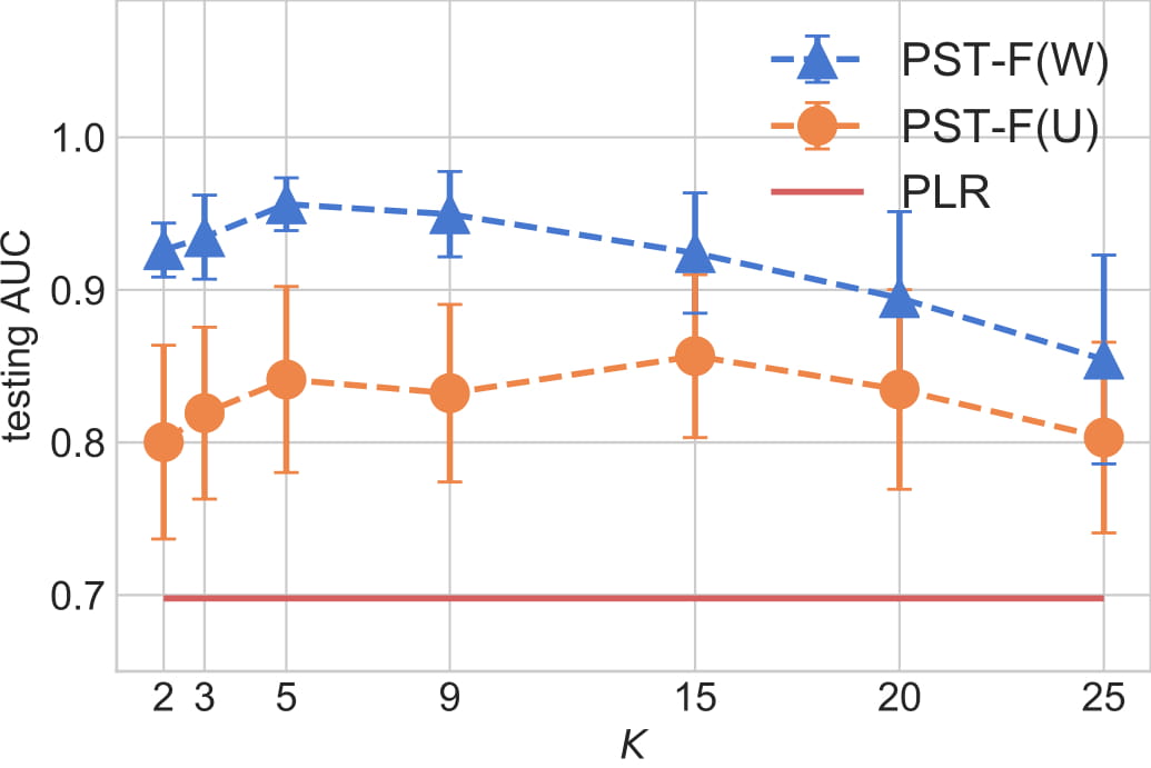
(a) MNIST.

(b) NEWS20.

Figure 2: Testing AUC at different $K$’s.

3). Changing the Feature Importance. In the above experiments, feature importance is defined based on the variance from PCA. Here, we show how feature importance influences prediction performance. In real-world applications, we may not know the exact importance of features. Thus, we replace variance $v_{i}$ by the $i$th power of $\alpha$ ($\alpha^{i}$), where $\alpha$ is a positive constant, and use (6) for assigning weights. Note that when $\alpha\!<\!1$, more importance features have larger weights; and vice versa when $\alpha\!>\!1$. Note that PST-F(W) does not reduce to PST-F(U) when $\alpha=1$, as more important features are still grouped together.

branch#	1	2	3	4	5	6	7	8
PST-H(W)	0.747$\pm$0.032	0.736$\pm$0.032	0.740$\pm$0.040	0.714$\pm$0.040	0.766$\pm$0.039	0.707$\pm$0.017	0.721$\pm$0.0464	0.753$\pm$0.042
PST-H(U)	0.678$\pm$0.049	0.724$\pm$0.037	0.652$\pm$0.103	0.708$\pm$0.033	0.653$\pm$0.070	0.663$\pm$0.036	0.682$\pm$0.0336	0.692$\pm$0.044
PPHTL	0.602$\pm$0.085	0.608$\pm$0.078	0.528$\pm$0.062	0.563$\pm$0.067	0.577$\pm$0.075	0.601$\pm$0.031	0.580$\pm$0.0708	0.583$\pm$0.056
PLR(target)	0.548$\pm$0.088	0.620$\pm$0.055	0.636$\pm$0.046	0.579$\pm$0.075	0.533$\pm$0.058	0.613$\pm$0.035	0.561$\pm$0.0764	0.584$\pm$0.045
branch#	9	10	11	12	13	14	15	16
PST-H(W)	0.701$\pm$0.023	0.698$\pm$0.036	0.736$\pm$0.046	0.738$\pm$0.045	0.746$\pm$0.0520	0.661$\pm$0.094	0.697$\pm$0.023	0.604$\pm$0.012
PST-H(U)	0.635$\pm$0.026	0.644$\pm$0.050	0.635$\pm$0.054	0.645$\pm$0.061	0.718$\pm$0.0647	0.644$\pm$0.044	0.647$\pm$0.061	0.567$\pm$0.036
PPHTL	0.547$\pm$0.066	0.517$\pm$0.075	0.565$\pm$0.059	0.547$\pm$0.089	0.592$\pm$0.0806	0.615$\pm$0.071	0.558$\pm$0.065	0.524$\pm$0.027
PLR(target)	0.515$\pm$0.065	0.555$\pm$0.061	0.553$\pm$0.066	0.520$\pm$0.088	0.619$\pm$0.0701	0.563$\pm$0.026	0.558$\pm$0.060	0.517$\pm$0.053

Table 2: Testing AUC on all branches of RUIJIN data set. The best and comparable results according to pair-wise 95% significance test are high-lighted. Testing AUC of PLR on main center is 0.668$\pm$0.026.

Figure 3 shows the testing AUCs at different $\alpha$’s. As can be seen, with proper assigned weights (i.e., $\alpha<1$ and more important features have larger $q_{k}$’s), the testing AUC can get higher. If less important features are more valued, the testing AUC decreases and may not be better than PST-F(U), which uses uniform weights. Moreover, we see that PST-F(W) is not sensitive to the weights once they are properly assigned.

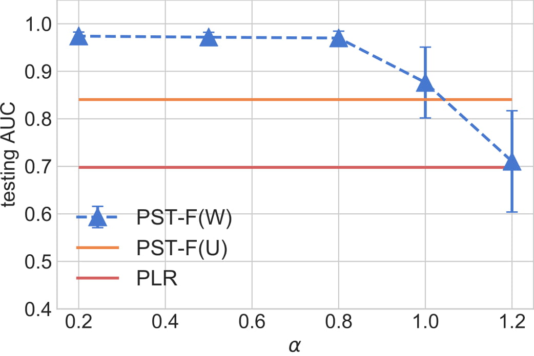
(a) MNIST.

(b) NEWS20.

Figure 3: Testing AUC with different feature importance settings.

4). Choice of High-Level Model. In this section, we compare different high-level models in combining predictions from the low-level models. The following methods are compared: (i) major voting (C-mv) from low-level models; (ii) weighted major voting (C-wmv), which uses $\{q_{k}\}$ as the weights; and (iii) by a high-level model in PST-F (denoted “C-hl”). Figure 4 shows results on NEWS20 with $\epsilon\!=\!1.0$. As can be seen, C-0 in Figure 4(b) has the best performance among all single low-level models, as it contains the most important features. Besides, stacking (i.e., C-hl), is the best way to combine predictions from C-{0-4}, which also offers better performance than any single low-level models.

(a) PST-F(U).

(b) PST-F(W).

Figure 4: Testing AUC of low-levels models and different combining methods on NEWS20 ($\epsilon=1.0$), where C-0 to C-4 are performance of low-level models.

4.2 Diabetes Prediction

1). Background. Diabetes is a group of metabolic disorders with high blood sugar levels over a prolonged period. From 2012 to 2015, approximately 1.5 to 5 million deaths each year are resulted from diabetes. Thus, prevention and diagnosis of diabetes are of great importance. The RUIJIN diabetes data set is collected by the Shanghai Ruijin Hospital during two investigations (in 2010 and 2013), conducted by the main hospital in Shanghai and 16 branches across China. The first investigation consists of questionnaires and laboratory tests collecting demographics, life-styles, disease information, and physical examination results. The second investigation includes diabetes diagnosis. Some collected features are shown in Table 3. Table 4 shows a total of 105,763 participants who appear in both two investigations. The smaller branches may not have sufficient labeled medical records for good prediction. Hence, it will be useful to borrow knowledge learned by the main hospital. However, users’ privacy is a major concern, and patients’ personal medical records in the main hospital should not be leaked to the branches.

name	importance	explaination
mchild	0.010	number of children
weight	0.012	birth weight
bone	0.013	bone mass measurement
eggw	0.005	frequency of having eggs
Glu120	0.055	glucose level 2 hours after meals
Glu0	0.060	glucose level immediately after meals
age	0.018	age
bmi	0.043	body mass index
HDL	0.045	high-density lipoprotein

Table 3: Some features in the RUIJIN data set, and importance is suggested by doctors. Top (resp. bottom) part: Features collected from the first (resp. second) investigation.

main	#1	#2	#3	#4	#5	#6	#7	#8
12,702	4,334	4,739	6,121	2,327	5,619	6,360	4,966	5,793
	#9	#10	#11	#12	#13	#14	#15	#16
	6,215	3,659	5,579	2,316	4,285	6,017	6,482	4,493

Table 4: Number of samples collected from the main hospital and 16 branches in the RUIJIN data set.

Setup. In this section, we apply the method in Section 3.3 for diabetes prediction. Specifically, based on the patient data collected during the first investigation in 2010, we predict whether he/she will have diabetes diagnosed in 2013. The main hospital serves as the source domain, and the branches are the target domains. We set $\epsilon_{\text{src}}=\epsilon_{\text{tgt}}=1.0$. The following methods are also compared: (i) PLR(target), which directly uses PLR on the target data; (ii) PPHTL Wang et al. (2018): a recently proposed privacy-preserving HTL method based on PLR; (iii) PST-F(U): There are 50 features, and they are randomly split into five groups, i.e., $K=5$, and each group have equal weights; (iv) PST-F(W): Features are first sorted by importance, and then grouped as follows: The top 10 features are placed in the first group, the next 10 features go to the second group, and so on. $q^{k}$ is set based on (6), with $v_{i}$ being the importance values provided by the doctors. The other settings are the same as in Section 4.1.

2). Results. Results are shown in Table 2. PPHTL may not have better performance than PLR(target), which is perhaps due to noise introduced in features. However, PST-F(U) improves over PPHTL by feature splitting, and consistently outperforms PLR(target). PST-F(W), which considers features importance, is the best.

5 Conclusion

In this paper, we propose a new privacy-preserving machine learning method, which improves privacy-preserving logistic regression by stacking. This can be done by either sample-based or feature-based partitioning of the data set. We provide theoretical justifications that the feature-based approach is better and requires a smaller sample complexity. Besides, when the importance of features is available, this can further boost the feature-based approach both in theory and practice. Effectiveness of the proposed method is verified on both standard benchmark data sets and a real-world cross-organizational diabetes prediction application. As a future work, we will extend the proposed algorithm to other classifiers, such as decision tree and deep networks.

Appendix A Proof

Notation. Given two datasets $\mathcal{D}$ and $\mathcal{D}^{\prime}$, $|\mathcal{D}-\mathcal{D}^{\prime}|=1$ denotes that $\mathcal{D}$ and $\mathcal{D}^{\prime}$ differ only $1$ sample. Let $J({\bm{\mathbf{w}}}\rightarrow{\bm{\mathbf{b}}}|\mathcal{D})$ denote the Jacobian matrix of the mapping from ${\bm{\mathbf{w}}}$ to ${\bm{\mathbf{b}}}$, when the dataset is $\mathcal{D}$. Let $\bar{F}({\bm{\mathbf{w}}};\mathcal{D},{\bm{\mathbf{b}}},\Delta)$ denote $\sum_{\{{\bm{\mathbf{x}}}_{i},y_{i}\}\in\mathcal{D}}\ell({\bm{\mathbf{w}}}^{\top}{\bm{\mathbf{x}}}_{i},y_{i})+\frac{1}{n}{\bm{\mathbf{b}}}^{\top}{\bm{\mathbf{w}}}+\frac{1}{2}\Delta\|{\bm{\mathbf{w}}}\|^{2}$, where $n$ is the number of samples in $\mathcal{D}$.

A.1 Proposition 3

Proof.

Note that we apply PLR algorithm with privacy budget $\epsilon$ on $\mathcal{S}_{k}$, so ${\bm{\mathbf{w}}}_{k}^{l}$ is $\epsilon$-differentially private for $\mathcal{S}_{k}$. We apply PLR algorithm on meta-data $\mathcal{M}^{s}$. So we have

$$\frac{\text{Pr}({\bm{\mathbf{w}}}^{h}|\mathcal{D}^{h})}{\text{Pr}({\bm{\mathbf{w}}}^{h}|\mathcal{D}^{\prime h})}=\frac{\text{Pr}({\bm{\mathbf{w}}}^{h}|\mathcal{M}^{s})}{\text{Pr}({\bm{\mathbf{w}}}^{h}|\mathcal{M}_{s})}=\epsilon.$$

Since $\{\mathcal{S}_{1},\mathcal{S}_{2},\ldots,\mathcal{S}_{K},\mathcal{D}^{h}\}$ are disjoint subsets, according to Theorem 4 in McSherry and Mironov (2009), $\{\{{\bm{\mathbf{w}}}^{l}_{k}\},{\bm{\mathbf{w}}}^{h}\}$ is $\epsilon$-differentially private. ∎

A.2 Theorem 4

To prove Theorem 4, we first prove the following Lemma 7 and 8. Without of generality, we assume $g$ is of $1$-strongly convex in the sequel.

Lemma 7.

For a dataset $\mathcal{D}$ and a vector ${\bm{\mathbf{b}}}$, assume that $\ell$ is differentiable and continuous with $|\ell^{\prime}(z)|\leq 1$, and $|\ell^{\prime\prime}(z)|\leq c$ for all $z$, and $g$ is $1$-strongly convex, $\|{\bm{\mathbf{x}}}_{i}\|\leq q$ for all ${\bm{\mathbf{x}}}_{i}\in\mathcal{D}$. Let $\mathcal{D}$ and $\mathcal{D}^{\prime}$ be the two datasets which differ in the value of the $n$-th item such that

$$\mathcal{D} =\{({\bm{\mathbf{x}}}_{1},y_{1}),\dots,({\bm{\mathbf{x}}}_{n-1},y_{n-1}),({\bm{\mathbf{x}}}_{n},y_{n})\},$$ (7)

$$\mathcal{D}^{\prime} =\{({\bm{\mathbf{x}}}_{1},y_{1}),\dots,({\bm{\mathbf{x}}}_{n-1},y_{n-1}),({\bm{\mathbf{x}}}^{\prime}_{n},y^{\prime}_{n})\},$$ (8)

Moreover, let ${\bm{\mathbf{b}}}$ and ${\bm{\mathbf{b}}}^{\prime}$ be two vectors such that

$$\begin{split}\bar{\bm{\mathbf{w}}}&=\arg\min_{{\bm{\mathbf{w}}}}\bar{F}({\bm{\mathbf{w}}};\mathcal{D},{\bm{\mathbf{b}}},\Delta)+\lambda g({\bm{\mathbf{w}}})\\ &=\arg\min_{{\bm{\mathbf{w}}}}\bar{F}({\bm{\mathbf{w}}};\mathcal{D}^{\prime},{\bm{\mathbf{b}}}^{\prime},\Delta)+\lambda g({\bm{\mathbf{w}}})\end{split}$$

For any $\Delta\geq 0$, we have

$$\frac{|\text{det}(J(\bar{{\bm{\mathbf{w}}}}\rightarrow{\bm{\mathbf{b}}}^{\prime}|\mathcal{D}^{\prime}))|}{|\text{det}(J(\bar{{\bm{\mathbf{w}}}}\rightarrow{\bm{\mathbf{b}}}|\mathcal{D}))|}\leq\left(1+\frac{q^{2}c}{n(\lambda+\Delta)}\right)^{2},$$ (9)

and

$$\|{\bm{\mathbf{b}}}\|-\|{\bm{\mathbf{b}}}^{\prime}\|\leq 2q.$$ (10)

Proof.

We take the gradient of $F$ to $0$ at $\bar{{\bm{\mathbf{w}}}}$, and can obtain

$${\bm{\mathbf{b}}}=-n\lambda\Delta g(\bar{{\bm{\mathbf{w}}}})-\sum_{i}^{n}y_{i}\ell^{\prime}(y_{i}{\bm{\mathbf{x}}}_{i}^{\top}\bar{{\bm{\mathbf{w}}}}){\bm{\mathbf{x}}}-n\Delta\bar{{\bm{\mathbf{w}}}}$$

Moreover, define matrices $A$ and $E$ as follows:

$$A =n\lambda\nabla^{2}g(\bar{{\bm{\mathbf{w}}}})+\sum_{i=1}^{n}y_{i}^{2}\ell^{\prime\prime}(y_{i}{\bm{\mathbf{x}}}^{\top}_{i}\bar{{\bm{\mathbf{w}}}}){\bm{\mathbf{x}}}_{i}{\bm{\mathbf{x}}}_{i}^{\top}+n\Delta I_{d},$$ (11)

$$E =-y_{i}^{2}\ell^{\prime\prime}(y_{i}{\bm{\mathbf{x}}}^{\top}_{i}\bar{{\bm{\mathbf{w}}}}){\bm{\mathbf{x}}}_{i}{\bm{\mathbf{x}}}_{i}^{\top}+(y^{\prime}_{n})^{2}\ell^{\prime\prime}(y^{\prime}_{n}{\bm{\mathbf{x}}}^{\prime\top}_{i}\bar{{\bm{\mathbf{w}}}}){\bm{\mathbf{x}}}_{n}^{\prime}{\bm{\mathbf{x}}}_{n}^{\prime\top}$$ (12)

From the proof of Theorem 9 in Chaudhuri et al. (2011) we know

$$\begin{split}&\frac{|\text{det}(J(\bar{{\bm{\mathbf{w}}}}\rightarrow{\bm{\mathbf{b}}}^{\prime}|\mathcal{D}^{\prime}))|}{|\text{det}(J(\bar{{\bm{\mathbf{w}}}}\rightarrow{\bm{\mathbf{b}}}|\mathcal{D}))|}\\ &=|1+\tau_{1}(A^{-1}E)+\tau_{2}(A^{-1}E)+\tau_{1}(A^{-1}E)\tau_{2}(A^{-1}E)|,\end{split}$$

where $\tau_{1}(),\tau_{2}()$ denote the largest and second largest eigenvalues of a matrix. Applying the triangle inequality of trace norm,

$$\begin{split}|\tau_{1}(E)|+|\tau_{2}(E)|\leq&|y_{n}^{2}\ell^{\prime\prime}(y_{n}{\bm{\mathbf{x}}}_{n}^{\top}\bar{{\bm{\mathbf{w}}}})|\|{\bm{\mathbf{x}}}_{n}\|^{2}\\ &+|-(y^{\prime}_{n})^{2}\ell^{\prime\prime}(y_{n}{\bm{\mathbf{x}}}_{n}^{\prime\top}\bar{{\bm{\mathbf{w}}}})|\|{\bm{\mathbf{x}}}_{n}^{\prime}\|^{2}\end{split}$$

Then upper bounds on $|y_{i}|$, $\|{\bm{\mathbf{x}}}_{i}\|$, and $|\ell^{\prime\prime}(z)|$ yield

$$|\tau_{1}(E)|+|\tau_{2}(E)|\leq 2cq^{2}.$$

Therefore $|\tau_{1}(E)|\cdot|\tau_{2}(E)|\leq c^{2}q^{4}$, and

$$\begin{split}&\frac{|\text{det}(J(\bar{{\bm{\mathbf{w}}}}\rightarrow{\bm{\mathbf{b}}}^{\prime}|\mathcal{D}^{\prime}))|}{|\text{det}(J(\bar{{\bm{\mathbf{w}}}}\rightarrow{\bm{\mathbf{b}}}|\mathcal{D}))|}\\ &\leq 1+\frac{2cq^{2}}{n(\lambda+\Delta)}+\frac{c^{2}q^{4}}{n^{2}(\lambda+\Delta)^{2}}=\left(1+\frac{cq^{2}}{n(\lambda+\Delta)}\right)^{2}\end{split}$$

and we obtain (9). For ${\bm{\mathbf{b}}}$ and ${\bm{\mathbf{b}}}^{\prime}$, we have

$${\bm{\mathbf{b}}}^{\prime}-{\bm{\mathbf{b}}}=y_{n}\ell^{\prime}(y_{n}{\bm{\mathbf{x}}}^{\top}_{n}\bar{{\bm{\mathbf{w}}}}){\bm{\mathbf{x}}}_{n}-y^{\prime}_{n}\ell^{\prime}(y_{n}{\bm{\mathbf{x}}}_{n}^{\prime\top}\bar{{\bm{\mathbf{w}}}}){\bm{\mathbf{x}}}_{n}^{\prime}$$

Due to that of $|\ell^{\prime}(\cdot)|\leq 1$,$|y_{i}|\leq 1$, $\|{\bm{\mathbf{x}}}_{i}\|\leq q$, we have

$$\|{\bm{\mathbf{b}}}\|-\|{\bm{\mathbf{b}}}\|^{\prime}\leq\|{\bm{\mathbf{b}}}-{\bm{\mathbf{b}}}^{\prime}\|\leq 2q,$$

and we obtain (10). ∎

Lemma 8.

$\{{\bm{\mathbf{w}}}^{l}_{k}\}$ in Algorithm 3 is $\epsilon$-differentially private with dataset $\mathcal{D}^{l}$.

Proof.

For simplicity, in this proof we ignore the superscript $\cdot^{l}$. The proof follows the proof of Theorem $9$ in Chaudhuri et al. (2011). Let $\mathcal{D}$ and $\mathcal{D}^{\prime}$ be two datasets of size $n$ and $|\mathcal{D}-\mathcal{D}^{\prime}|=1$. So $|\mathcal{F}_{k}-\mathcal{F}^{\prime}_{k}|=1$ for all $k$. We have a set of optimization problems

$${\bm{\mathbf{w}}}_{k}=\arg\min_{{\bm{\mathbf{w}}}}\bar{F}({\bm{\mathbf{w}}};\mathcal{F}_{k},{\bm{\mathbf{b}}}_{k},\Delta_{k})+\lambda_{k}g_{k}({\bm{\mathbf{w}}}),\forall k.$$

Since ${{\bm{\mathbf{w}}}_{1},{\bm{\mathbf{w}}}_{2},\dots,{{\bm{\mathbf{w}}}}_{K}}$ are independent given the dataset, we have

$$\begin{split}&\frac{\text{Pr}(\{{\bm{\mathbf{w}}}_{k}\}^{K}_{k=1}|\mathcal{D})}{\text{Pr}(\{{\bm{\mathbf{w}}}_{(k)}\}^{K}_{k=1}|\mathcal{D}^{\prime})}=\prod_{k=1}^{K}\frac{\text{Pr}({\bm{\mathbf{w}}}_{k}|\mathcal{F}_{k})}{\text{Pr}({\bm{\mathbf{w}}}_{k}|\mathcal{F}_{k}^{\prime})}\\ &=\prod_{k=1}^{K}\frac{\text{Pr}({\bm{\mathbf{b}}}_{k}|\mathcal{F})}{\text{Pr}({\bm{\mathbf{b}}}^{\prime}_{k}|\mathcal{F}_{k}^{\prime})}\frac{\left|\text{det}(J_{k}({{\bm{\mathbf{w}}}}^{(k)}\rightarrow{\bm{\mathbf{b}}}_{k}|\mathcal{F}_{k}))\right|^{-1}}{\left|\text{det}(J_{k}({{\bm{\mathbf{w}}}}_{k}\rightarrow{\bm{\mathbf{b}}}^{\prime}_{k}|\mathcal{F}_{k}^{\prime}))\right|^{-1}}.\end{split}$$

By (9) in Lemma 7 with upper bound of sample norm $q^{(k)}$,

$$\frac{\left|\text{det}(J_{k}({{\bm{\mathbf{w}}}}_{k}\rightarrow{\bm{\mathbf{b}}}_{k}|\mathcal{F}_{k}))\right|^{-1}}{\left|\text{det}(J_{k}({{\bm{\mathbf{w}}}}_{(k)}\rightarrow{\bm{\mathbf{b}}}^{\prime}_{k}|\mathcal{F}_{k}^{\prime}))\right|^{-1}}\leq\left(1+\frac{c(q_{k})^{2}}{n(\lambda_{k}+\Delta_{k})}\right)^{2},$$

and

$$\frac{\text{Pr}({\bm{\mathbf{b}}}_{k}|\mathcal{D})}{\text{Pr}({\bm{\mathbf{b}}}^{\prime}_{k}|\mathcal{D}^{\prime})}\leq e^{\epsilon^{\prime}(\|{\bm{\mathbf{b}}}_{k}\|-\|{\bm{\mathbf{b}}}^{\prime}_{k}\|)/2}\leq e^{q_{k}\epsilon^{\prime}}.$$

Thus

$$\frac{\text{Pr}(\{{{\bm{\mathbf{w}}}}_{k}\}^{K}_{k=1}|\mathcal{D})}{\text{Pr}(\{{{\bm{\mathbf{w}}}}_{k}\}^{K}_{k=1}|\mathcal{D}^{\prime})}=e^{\epsilon^{\prime}}\prod_{k=1}^{K}\left(1+\frac{c(q_{k})^{2}}{n(\lambda_{k}+\Delta_{k})}\right)^{2}.$$

We know that for $\ell(\cdot)$, $c=\frac{1}{4}$. When $\Delta=0$, $\epsilon=\epsilon^{\prime}+\sum_{k=1}\log(1+\frac{(q_{k})^{2}}{2n\lambda_{k}}+\frac{(q_{k})^{4}}{16n^{2}(\lambda_{k})^{2}})$, we have

$$\frac{\text{Pr}(\{{\bm{\mathbf{w}}}_{k}\}^{K}_{k=1}|\mathcal{D})}{\text{Pr}(\{{{\bm{\mathbf{w}}}}_{k}\}^{K}_{k=1}|\mathcal{D}^{\prime})}=e^{\epsilon}.$$

When $\Delta>0$, by definition,

$$\prod_{k=1}^{K}\left(1+\frac{c(q_{k})^{2}}{n(\lambda_{k}+\Delta_{k})}\right)^{2}=\prod_{k=1}^{K}e^{q_{k}\epsilon/2}=e^{\epsilon/2},$$

$$\epsilon=\epsilon^{\prime}+\epsilon/2.$$

As a result,

$$\frac{\text{Pr}(\{{{\bm{\mathbf{w}}}}_{k}\}^{K}_{k=1}|\mathcal{D})}{\text{Pr}(\{{{\bm{\mathbf{w}}}}_{k}\}^{K}_{k=1}|\mathcal{D}^{\prime})}=e^{\epsilon}.$$

∎

Now we are ready to prove Theorem 4.

Proof.

From Lemma 8, we know that $\{{\bm{\mathbf{w}}}^{k}_{l}\}$ is $\epsilon$-differentially private for $\mathcal{D}_{l}$. Since we apply PLR on $\mathcal{M}^{f}$, we have

$$\frac{\text{Pr}({\bm{\mathbf{w}}}^{h}|\mathcal{D}^{h})}{\text{Pr}({\bm{\mathbf{w}}}^{h}|\mathcal{D}^{\prime h})}=\frac{\text{Pr}({\bm{\mathbf{w}}}^{h}|\mathcal{M}^{f})}{\text{Pr}({\bm{\mathbf{w}}}^{h}|\mathcal{M}^{\prime f})}=\epsilon.$$

So ${\bm{\mathbf{w}}}^{h}$ is $\epsilon$-differentially private for $\mathcal{D}^{h}$. Since $\mathcal{D}^{l}$ and $\mathcal{D}^{h}$ are disjoint subsets, according to Theorem 4 in McSherry and Mironov (2009), $\{\{{\bm{\mathbf{w}}}^{l}_{k}\},{\bm{\mathbf{w}}}^{h}\}$ is $\epsilon$-differentially private for $\mathcal{D}$. ∎

A.3 Theorem 5

Proof.

For simplicity, we omit the superscript $\cdot^{l}$. Suppose the samples in $\mathcal{F}$ are i.i.d. drawn according to $P_{k}$. We define

$$F_{k}({\bm{\mathbf{w}}},\mathcal{D}) =\frac{1}{n}\sum_{({\bm{\mathbf{x}}}_{i},y_{i})\in\mathcal{F}_{k}}\ell({\bm{\mathbf{w}}}^{\top}{\bm{\mathbf{x}}}_{i},y_{i})+\lambda_{k}g_{k}({\bm{\mathbf{w}}}),$$ (13)

$$\tilde{F}_{k}({\bm{\mathbf{w}}}) =L({\bm{\mathbf{w}}},P_{k})+\frac{\lambda_{k}}{2}\|{\bm{\mathbf{w}}}\|^{2}.$$ (14)

and let

$$\tilde{{\bm{\mathbf{w}}}}_{k} =\arg\min_{{\bm{\mathbf{w}}}}\tilde{F}_{k}({\bm{\mathbf{w}}})$$ (15)

$$({\bm{\mathbf{w}}}_{k})^{*} =\arg\min_{{\bm{\mathbf{w}}}}F_{k}({\bm{\mathbf{w}}},\mathcal{D}).$$ (16)

The results in proof of Theorem 18 in Chaudhuri et al. (2011) shows

$$L({{\bm{\mathbf{w}}}}_{k})= L({{\bm{\mathbf{v}}}}_{k})+(\tilde{F}_{k}({{\bm{\mathbf{w}}}}_{k})-\tilde{F}_{k}(\tilde{{\bm{\mathbf{w}}}}_{k}))$$ (17)

$$+(\tilde{F}_{k}(\tilde{{\bm{\mathbf{w}}}}_{k})-\tilde{F}_{k}({\bm{\mathbf{v}}}_{k}))+\frac{\lambda_{k}}{2}\|{\bm{\mathbf{v}}}_{k}\|^{2}-\frac{\lambda_{k}}{2}\|{{\bm{\mathbf{w}}}}_{k}\|^{2}.$$

Let $s_{k}=\|{\bm{\mathbf{v}}}_{k}\|$ If $n>\frac{q_{k}(s_{k})^{2}}{\epsilon_{g}\epsilon}$ and $\lambda_{k}>\frac{\epsilon_{g}}{(s_{k})^{2}}$, then $n\lambda_{k}>\frac{q_{k}}{\epsilon}$, from the definition of $\epsilon^{\prime}$ in Algorithm 3,

$$\begin{split}\epsilon^{\prime}&=\epsilon-2\prod_{k=1}^{K}\log(1+\frac{(q_{k})^{2}}{4n\lambda_{k}})\\ &=\epsilon-2\prod_{k=1}^{K}\log(1+\frac{q_{k}\epsilon}{4})\geq\epsilon-\frac{\epsilon}{2},\end{split}$$

where the last step is from the inequality $\log(1+x)<x$ for $x\in[0,1]$.

From the Lemma $19$ in Chaudhuri et al. (2011), we have that with probability at least $1-\delta$,

$$F_{k}({{\bm{\mathbf{w}}}}_{k},\mathcal{D})-F_{k}(({{\bm{\mathbf{w}}}}_{k})^{*},\mathcal{D})\leq\frac{4d^{2}\log^{2}(d/(K\delta))(q_{k})^{2}}{\lambda_{k}n^{2}\epsilon^{2}}.$$

From Sridharan et al. (2009),

$$\begin{split}&\tilde{F}_{k}({\bm{\mathbf{w}}}_{k})-\tilde{F}_{k}(\tilde{{\bm{\mathbf{w}}}}_{k})\\ &\leq 2(F_{k}({{\bm{\mathbf{w}}}}_{k},\mathcal{D})-F_{k}(({{\bm{\mathbf{w}}}}_{k})^{*},\mathcal{D}))+\mathcal{O}(\frac{\log(1/\delta)}{K^{2}\lambda_{k}n})\\ &\leq\frac{8d^{2}\log^{2}(d/(K\delta))}{K^{2}\lambda_{k}n^{2}\epsilon^{2}}+\mathcal{O}(\frac{(q_{k})^{2}\log(1/\delta)}{\lambda_{k}n}).\end{split}$$

By definition of $\tilde{{\bm{\mathbf{w}}}}_{k}$, we have $\tilde{F}(\tilde{\bm{\mathbf{w}}}_{k})-\tilde{F}({\bm{\mathbf{v}}}_{k})\leq 0$. If $\lambda_{k}=\frac{\epsilon_{g}}{(s_{k})^{2}}$, then the $4$th term in (17) is at most $\frac{\epsilon_{g}}{2}$. Finally, the Theorem follows by solving for $n$ to make the total excess error at most $\epsilon_{g}$. ∎

References

- Abadi et al. [2016] M. Abadi, A. Chu, I. Goodfellow, B. McMahan, I. Mironov, K. Talwar, and L. Zhang. Deep learning with differential privacy. In SIGSAC, pages 308–318. ACM, 2016.
- Bassily et al. [2014] R. Bassily, A. Smith, and A. Thakurta. Private empirical risk minimization: Efficient algorithms and tight error bounds. In FOCS, pages 464–473. IEEE, 2014.
- Boyd et al. [2011] S. Boyd, N. Parikh, and E. Chu. Distributed optimization and statistical learning via the alternating direction method of multipliers. Foundations and Trends® in Machine learning, 3(1):1–122, 2011.
- Breiman [1996a] L. Breiman. Bagging predictors. Machine Learning, 24(2):123–140, 1996.
- Breiman [1996b] L. Breiman. Stacked regressions. Machine Learning, 24(1):49–64, 1996.
- Chaudhuri et al. [2011] K. Chaudhuri, C. Monteleoni, and A. Sarwate. Differentially private empirical risk minimization. JMLR, 12(Mar):1069–1109, 2011.
- Dwork and Roth [2014] C. Dwork and A. Roth. The algorithmic foundations of differential privacy. Foundations and Trends® in Theoretical Computer Science, 9(3–4):211–407, 2014.
- Dwork et al. [2006] C. Dwork, F. McSherry, K. Nissim, and A. Smith. Calibrating noise to sensitivity in private data analysis. In TCC, pages 265–284. Springer, 2006.
- Džeroski and Ženko [2004] S. Džeroski and B. Ženko. Is combining classifiers with stacking better than selecting the best one? Machine learning, 54(3):255–273, 2004.
- Emekçi et al. [2007] F. Emekçi, O. Sahin, D. Agrawal, and A. El Abbadi. Privacy preserving decision tree learning over multiple parties. TKDE, 63(2):348–361, 2007.
- Fong and Weber-Jahnke [2012] P. Fong and J. Weber-Jahnke. Privacy preserving decision tree learning using unrealized data sets. TKDE, 24(2):353–364, 2012.
- Friedman et al. [2000] J. Friedman, T. Hastie, and R. Tibshirani. Additive logistic regression: a statistical view of boosting. Annals of Statistics, 28(2):337–407, 2000.
- Friedman et al. [2012] J. Friedman, T. Hastie, and R. Tibshirani. The elements of statistical learning. Springer, 2012.
- Hamm et al. [2016] J. Hamm, Y. Cao, and M. Belkin. Learning privately from multiparty data. In ICML, pages 555–563, 2016.
- Hanley and McNeil [1983] J. Hanley and B. McNeil. A method of comparing the areas under receiver operating characteristic curves derived from the same cases. Radiology, 148(3):839–843, 1983.
- Kasiviswanathan and Jin [2016] P. Kasiviswanathan and H. Jin. Efficient private empirical risk minimization for high-dimensional learning. In ICML, pages 488–497, 2016.
- Kifer et al. [2012] D. Kifer, A. Smith, and A. Thakurta. Private convex empirical risk minimization and high-dimensional regression. JMLR, 23, 2012.
- Kuzborskij and Orabona [2013] I. Kuzborskij and F. Orabona. Stability and hypothesis transfer learning. In ICML, pages 942–950, 2013.
- Lang [1995] Ken Lang. Newsweeder: Learning to filter netnews. In ICML. Citeseer, 1995.
- LeCun et al. [1998] Y. LeCun, L. Bottou, Y. Bengio, and P. Haffner. Gradient-based learning applied to document recognition. Proceedings of the IEEE, 86(11):2278–2324, 1998.
- McSherry and Mironov [2009] F. McSherry and I. Mironov. Differentially private recommender systems: Building privacy into the netflix prize contenders. In SIGKDD, pages 627–636, 2009.
- Ozay and Vural [2012] M. Ozay and F. Vural. A new fuzzy stacked generalization technique and analysis of its performance. Technical report, arXiv:1204.0171, 2012.
- Pan and Yang [2010] J. Pan and Q. Yang. A survey on transfer learning. TKDE, 22(10):1345–1359, 2010.
- Papernot et al. [2017] N. Papernot, M. Abadi, U. Erlingsson, I. Goodfellow, and K. Talwar. Semi-supervised knowledge transfer for deep learning from private training data. In ICLR, 2017.
- Pathak et al. [2010] M. Pathak, S. Rane, and B. Raj. Multiparty differential privacy via aggregation of locally trained classifiers. In NeurIPS, pages 1876–1884, 2010.
- Rajkumar and Agarwal [2012] A. Rajkumar and S. Agarwal. A differentially private stochastic gradient descent algorithm for multiparty classification. In AISTAT, pages 933–941, 2012.
- Shalev-Shwartz and Srebro [2008] S. Shalev-Shwartz and N. Srebro. SVM optimization: inverse dependence on training set size. In ICML, pages 928–935. ACM, 2008.
- Shokri and Shmatikov [2015] R. Shokri and V. Shmatikov. Privacy-preserving deep learning. In SIGSAC, pages 1310–1321, 2015.
- Smyth and Wolpert [1999] P. Smyth and D. Wolpert. Linearly combining density estimators via stacking. Machine Learning, 36(1-2):59–83, 1999.
- Sridharan et al. [2009] Karthik Sridharan, Shai Shalev-Shwartz, and Nathan Srebro. Fast rates for regularized objectives. In NIPS, pages 1545–1552, 2009.
- Ting and Witten [1999] K. Ting and I. Witten. Issues in stacked generalization. JAIR, 10:271–289, 1999.
- Wang et al. [2018] Y. Wang, Q. Gu, and D. Brown. Differentially private hypothesis transfer learning. In ECML, 2018.
- Wolpert [1992] D. Wolpert. Stacked generalization. Neural Networks, 5(2):241–259, 1992.
- Xie et al. [2017] L. Xie, I. Baytas, K. Lin, and J. Zhou. Privacy-preserving distributed multi-task learning with asynchronous updates. In SIGKDD, pages 1195–1204, 2017.
- Zhou [2012] Z.-H. Zhou. Ensemble methods: foundations and algorithms. Chapman and Hall/CRC, 2012.