Practical optimal registration of terrestrial LiDAR scan pairs

Abstract

Point cloud registration is a fundamental problem in 3D scanning. In this paper, we address the frequent special case of registering terrestrial LiDAR scans (or, more generally, levelled point clouds). Many current solutions still rely on the Iterative Closest Point (ICP) method or other heuristic procedures, which require good initializations to succeed and/or provide no guarantees of success. On the other hand, exact or optimal registration algorithms can compute the best possible solution without requiring initializations; however, they are currently too slow to be practical in realistic applications.

Existing optimal approaches ignore the fact that in routine use the relative rotations between scans are constrained to the azimuth, via the built-in level compensation in LiDAR scanners. We propose a novel, optimal and computationally efficient registration method for this 4DOF scenario. Our approach operates on candidate 3D keypoint correspondences, and contains two main steps: (1) a deterministic selection scheme that significantly reduces the candidate correspondence set in a way that is guaranteed to preserve the optimal solution; and (2) a fast branch-and-bound (BnB) algorithm with a novel polynomial-time subroutine for 1D rotation search, that quickly finds the optimal alignment for the reduced set. We demonstrate the practicality of our method on realistic point clouds from multiple LiDAR surveys.

1 Introduction

LiDAR scanners are a standard instrument in contemporary surveying practice. An individual scan produces a 3D point cloud, consisting of densely sampled, polar line-of-sight measurements of the instrument’s surroundings, up to some maximum range. Consequently, a recurrent basic task in LiDAR surveying is to register individual scans into one big point cloud that covers the entire region of interest. The fundamental operation is the relative alignment of a pair of scans. Once this can be done reliably, it can be applied sequentially until all scans are registered; normally followed by a simultaneous refinement of all registration parameters.

Our work focuses on the pairwise registration: given two point clouds, compute the rigid transformation that brings them into alignment. Arguably the most widely used method for this now classical problem is the ICP (Iterative Closest Point) algorithm (Besl and McKay, 1992; Rusinkiewicz and Levoy, 2001; Pomerleau et al., 2013), which alternates between finding nearest-neighbour point matches and updating the transformation parameters. Since the procedure converges only to a local optimum, it requires a reasonably good initial registration to produce correct results.

Existing industrial solutions, which are shipped either as on-board software of the scanner itself, or as part of the manufacturer’s offline processing software (e.g., Zoller + Fröhlich, Riegl, Leica), rely on external aids or additional sensors. For instance, a GNSS/IMU sensor package, or a visual-inertial odometry system with a panoramic camera (Houshiar et al., 2015) setup, to enable scan registration in GNSS-denied environments, in particular indoors and under ground. Another alternative is to determine the rotation with a compass, then perform only a translation search, which often succeeds from a rough initialisation, such as setting the translation to $0$. Another, older but still popular approach is to install artificial targets in the environment (Akca, 2003; Franaszek et al., 2009) that act as easily detectable and matchable “beacons”. However, this comes at the cost of installing and maintaining the targets.

More sophisticated point cloud registration techniques have been proposed that are not as strongly dependent on good initializations, e.g., (Chen et al., 1999; Drost et al., 2010; Albarelli et al., 2010; Theiler et al., 2014, 2015). These techniques, in particular the optimization routines they employ, are heuristic. They often succeed, but cannot guarantee to find an optimal alignment (even according to their own definition of optimality). Moreover, such methods typically are fairly sensitive to the tuning of somewhat unintuitive, input-specific parameters, such as the approximate proportion of overlapping points in 4PCS (Aiger et al., 2008), or the annealing rate of the penalty component in the lifting method of (Zhou et al., 2016). In our experience, when applied to new, unseen registration tasks these methods often do not reach the performance reported on popular benchmark datasets.

In contrast to the locally convergent algorithms and heuristics above, optimal algorithms have been developed for point cloud registration (Breuel, 2001; Yang et al., 2016; Campbell and Petersson, 2016; Parra Bustos et al., 2016). Their common theme is to set up a clear-cut, transparent objective function and then apply a suitable exact optimization scheme – often branch-and-bound type methods – to find the solution that maximises the objective function. It is thus ensured that the best registration parameters (according to the adopted objective function) will always be found. Importantly, convergence to the optimal value independent of the starting point implies that these methods do not require initialization. However, a serious limitation of optimal methods is that they are computationally much costlier (due to NP-hardness of most of the robust objective functions used in point cloud registration (Chin et al., 2018)), but also by the experiments in previous literatures, e.g., more than 4 h for only $\approx$ 350 points in (Parra Bustos et al., 2016), and even longer in (Yang et al., 2016). This makes them impractical for LiDAR surveying.

1.1 Our contributions

In this work, we aim to make optimal registration practical for terrestrial LiDAR scans.

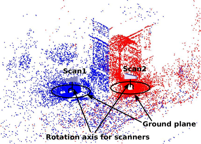
Figure 1: 4DOF registration of two LiDAR scans (blue and red). The level compensator forces scanners to rotate around the vertical axis, resulting in the azimuthal relative rotation.

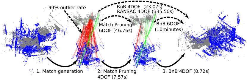
Figure 2: Method illustration. Given 2 point clouds (grey and blue), as shown by the solid arrows, we first generate a set of matches/candidate correspondences (only a subset is shown for visual clarity), which have both inliers (green) and outliers (red). The matches are quickly pruned without removing any inliers. Then, we run 4DOF BnB on the remaining matches to find the optimal solution. The dashed arrows show some alternative optimization choices. Note that our two-step process is much faster than directly optimising on the initial matches, and also more practically useful than its 6DOF counterpart (Bustos and Chin, 2017).

Towards that goal we make the following observations:

• Modern LiDAR devices are equipped with a highly accurate level compensator, which reduces the relative rotation between scans to the azimuth; see Figure 1. In most applications the search space therefore has only 4 degrees of freedom (DOF) rather than 6. This difference is significant, because the runtime of optimal methods grows very quickly with the problem dimension, see Figure 2.

• A small set of correspondences, i.e., correct point matches referring to close enough locations in the scene, is sufficient to reliably estimate the relative sensor pose, see Figure 2. The problem of match-based registration methods is normally not that there are too few correspondences to solve the problem; but rather that they are drowned in a large number of incorrect point matches, because of the high failure rate of existing 3D matching methods. The task would be a lot easier if we had a way to discard many false correspondences without losing true ones.

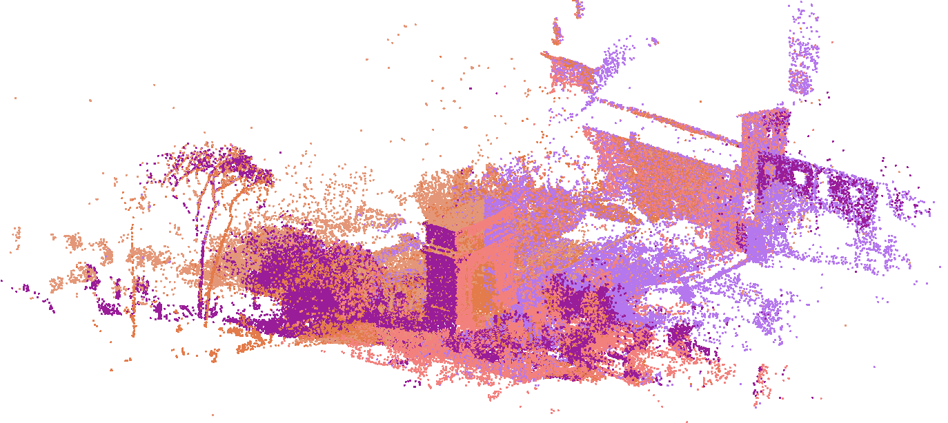
Figure 3: Registration result of our method for Arch dataset. The registration of all five scans (with 15k-20k input point matches per pair, not shown) takes 187.53s, without requiring manual initializations. Note that our main contribution in this paper is a fast optimal algorithm for registering LiDAR scan pairs. To register multiple scans (as achieved on the Arch dataset in this figure), we sequentially register the individual scans; see Section 3.2 for details.

On the basis of these observations we develop a novel method for optimal, match-based LiDAR registration, that has the following main steps:

• Instead of operating directly on the input match set, a fast deterministic preprocessing step is executed to aggressively prune the input set, in a way which guarantees that only false correspondences are discarded. In this way, it is ensured that the optimal alignment of the reduced set is the same as for the initial, complete set of matches.

• A fast 4DOF BnB algorithm is then run on the remaining matches to compute the optimal alignment parameters. Our BnB algorithm contains a deterministic polynomial-time subroutine for 1DOF rotation search, which accelerates the optimization.

Figure 2 illustrates our approach. As suggested in the figure and by our comprehensive testing (see Section 6), our approach significantly speeds up optimal registration and makes it practical for realistic LiDAR surveying tasks. For example, on the Arch dataset, it is able to accurately register all 5 scans in around 3 min without any initializations to the registration; see Figure 3.

Please visit our project homepage for the video demo and source code.

2 Related work

Point-based registration techniques can be broadly categorized into two groups: methods using “raw” point clouds, and methods using 3D point matches. Since our contribution belongs to the second group, we will focus our survey on that group. Nonetheless, in our experiments, we will compare against both raw point cloud methods and match-based methods.

Match-based methods first extract a set of candidate correspondences from the input point clouds (using feature matching techniques such as (Scovanner et al., 2007; Głomb, 2009; Zhong, 2009; Rusu et al., 2008, 2009)), then optimize the registration parameters using the extracted candidates only. Since the accuracy of 3D keypoint detection and matching is much lower than their 2D counterparts (Harris and Stephens, 1988; Lowe, 1999), a major concern of match-based methods is to discount the corrupting effects of false correspondences or outliers.

A widely used strategy for robust estimation is Random Sample Consensus (RANSAC) (Fischler and Bolles, 1981). However, the runtime of RANSAC increases exponentially with the outlier rate, which is generally very high in 3D registration,e.g., the input match set in Figure 2 contains more than $99\%$ outliers. More efficient approaches have been proposed for dealing with outliers in 3D match sets, such as the game-theoretic method of (Albarelli et al., 2010) and the lifting optimization method of (Zhou et al., 2016). However, these are either heuristic (e.g., using randomisation (Albarelli et al., 2010)) and find solutions that are, at most, correct with high probability, but may also be grossly wrong; or they are only locally optimal (Zhou et al., 2016), and will fail when initialized outside of the correct solution’s convergence basin.

Optimal algorithms for match-based 3D registration also exist (Bazin et al., 2012; Bustos and Chin, 2017; Yu and Ju, 2018). However, (Bazin et al., 2012) is restricted to pure rotational motion, while the 6DOF algorithms of (Bustos and Chin, 2017; Yu and Ju, 2018) are computationally expensive for unfavourable configurations. E.g., (Bustos and Chin, 2017) takes more than 10 min to register the pair of point clouds in Figure 2.

Recently, clever filtering schemes have been developed (Svarm et al., 2014; Parra Bustos and Chin, 2015; Chin and Suter, 2017; Bustos and Chin, 2017) which have the ability to efficiently prune a set of putative correspondences and only retain a much smaller subset, in a manner that does not affect the optimal solution (more details in Section 5). Our method can be understood as an extension of the 2D rigid registration method of (Chin and Suter, 2017, Section 4.2.1) to the 4DOF case.

Beyond points, other geometric primitives (lines, planes, etc.) have also been exploited for LiDAR registration (Brenner and Dold, 2007; Rabbani et al., 2007). By using more informative order structures in the data, such methods can potentially provide more accurate registration. Developing optimal registration algorithms based on higher-order primitives would be interesting future work.

3 Problem formulation

Given two input point clouds $\mathbf{P}$ and $\mathbf{Q}$, we first extract a set of 3D keypoint matches $\mathcal{C}=\{(\mathbf{p}_{i},\mathbf{q}_{i})\}_{i=1}^{M}$ between $\mathbf{P}$ and $\mathbf{Q}$. This can be achieved using fairly standard means — Section 6.1 will describe our version of the procedure. Given $\mathcal{C}$, our task is to estimate the 4DOF rigid transformation

$$f(\mathbf{p}\mid\theta,\mathbf{t})=\mathbf{R}(\theta)\mathbf{p}+\mathbf{t},$$ (1)

parameterized by a rotation angle $\theta\in[0,2\pi]$ and translation vector $\mathbf{t}\in\mathbb{R}^{3}$, that aligns as many of the pairs in $\mathcal{C}$ as possible. Note that

$$\mathbf{R}(\theta)=\left[\begin{matrix}&\cos{\theta}&\sin{\theta}&0\\ &-\sin{\theta}&\cos{\theta}&0\\ &0&0&1\end{matrix}\right]$$ (2)

defines a rotation about the 3rd axis, which we assume to be aligned with gravity, expressing the fact that LiDAR scanners in routine use are levelled.

Since $\mathcal{C}$ contains outliers (false correspondences), $f$ must be estimated robustly. To this end, we seek the parameters $\theta,\mathbf{t}$ that maximize the objective

$$E(\theta,\mathbf{t}\mid\mathcal{C},\epsilon)=\sum_{i=1}^{M}\mathbb{I}\left(\lVert\mathbf{R}(\theta)\mathbf{p}_{i}+\mathbf{t}-\mathbf{q}_{i}\rVert\leq\epsilon\right),$$ (3)

where $\epsilon$ is the inlier threshold, and $\mathbb{I}$ is an indicator function that returns 1 if the input predicate is satisfied and 0 otherwise. Intuitively, (3) calculates the number of pairs in $\mathcal{C}$ that are aligned up to distance $\epsilon$ by $f(\mathbf{p}\mid\theta,\mathbf{t})$. Allowing alignment only up to $\epsilon$ is vital to exclude the influence of the outliers. Note that choosing the right $\epsilon$ is usually not an obstacle, since LiDAR manufacturers specify the precision of the device, which can inform the choice of an appropriate threshold. Moreover, given the fast performance of the proposed technique, one could conceivably run multiple rounds of registration with different $\epsilon$ and choose one based on the alignment residuals.

Our overarching aim is thus to solve the optimization problem

$$E^{*}=\underset{\theta,\mathbf{t}}{\text{max}}\ E(\theta,\mathbf{t}\mid\mathcal{C},\epsilon)$$ (4)

exactly or optimally; in other words we are searching for the angle and translation vector $\theta^{*},\mathbf{t}^{*}$ that yield the highest objective value $E^{*}=E(\theta^{*},\mathbf{t}^{*}\mid\mathcal{C},\epsilon)$. We note that in the context of registration, optimality is not merely an academic exercise. Incorrect local minima are a real problem, as amply documented in the literature on ICP and illustrated by regular failures of the automatic registration routines in production software.

3.1 Main algorithm

As shown in Algorithm 1, our approach to solve (4) optimally has two main steps: a deterministic pruning step to reduce $\mathcal{C}$ to a much smaller subset $\mathcal{C}^{\prime}$ while removing only matches that cannot be correct, hence preserving the optimal solution $\theta^{\ast},\mathbf{t}^{\ast}$ in $\mathcal{C}^{\prime}$ (Section 5); and a fast, custom-tailored BnB algorithm to search for $\theta^{*},\mathbf{t}^{*}$ in $\mathcal{C}^{\prime}$ (Section 4). For better flow of the presentation, we will describe the BnB algorithm first, before the pruning.

Algorithm 1 Main algorithm.

0:  Point clouds $\mathbf{P}$ and $\mathbf{Q}$ with 1D relative rotation, inlier threshold $\epsilon$.

1:  Extract match set $\mathcal{C}$ from $\mathbf{P}$ and $\mathbf{Q}$ (Section 6.1).

2:  Prune $\mathcal{C}$ into a smaller subset $\mathcal{C}^{\prime}$ (Section 5).

3:  Solve (4) on $\mathcal{C}^{\prime}$ to obtain registration parameters $\theta^{*},\mathbf{t}^{*}$ (Section 4).

4:  return  Optimal solution $\theta^{*},\mathbf{t}^{*}$.

3.2 Registering multiple scans

In some applications, registering multiple scans is required. For this purpose, we can first perform pair-wise registration to estimate the relative poses between consecutive scans. These pair-wise poses can then be used to initialize simultaneous multi-scan registration methods like the maximum-likelihood alignment of (Lu and Milios, 1997) and conduct further optimization.

To refrain from further polishing that would obfuscate the contribution made by our robust pair-wise registration, all multi-scan registration results in this paper are generated by sequential pair-wise registration only, i.e., starting from the initial scan, incrementally register the next scan to the current one using Algorithm 1. As shown in Figure 3 and later in Section 6.2, our results are already promising even without further refinement.

4 Fast BnB algorithm for 4DOF registration

To derive our fast BnB algorithm, we first rewrite (4) as

$$E^{\ast}=\underset{\mathbf{t}}{\text{max}}\ U(\mathbf{t}\mid\mathcal{C},\epsilon),$$ (5)

where

$$U(\mathbf{t}\mid\mathcal{C},\epsilon)=\underset{\theta}{\text{max}}\ E(\theta,\mathbf{t}\mid\mathcal{C},\epsilon).$$ (6)

It is not hard to see the equivalence of (4) and (5). The purpose of (5) is twofold:

• As we will see in Section (4.1), estimating $\theta$ given $\mathbf{t}$ can be accomplished deterministically in polynomial time, such that the optimization of $\theta$ can be viewed as “evaluating” the function $U(\mathbf{t}\mid\mathcal{C},\epsilon)$.

• By “abstracting away” the variable $\theta$ as in (5), the proposed BnB algorithm (Section 4.2) can be more conveniently formulated as searching over only the 3-dimensional translation space $\mathbb{R}^{3}$.

4.1 Deterministic rotation estimation

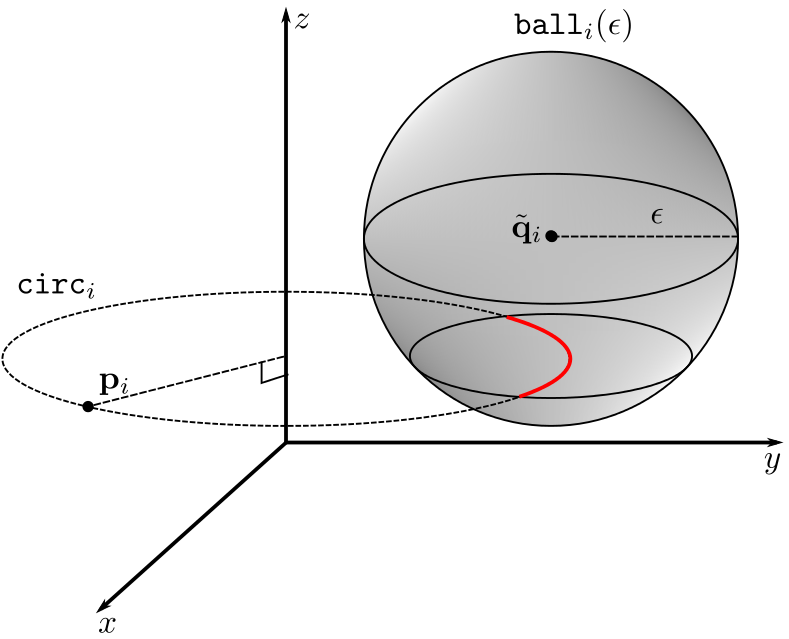
Figure 4: The intersection of $\mathtt{circ}_{i}$ and $\mathtt{ball}_{i}(\epsilon)$. The intersection part is rendered in red.

For completeness, the definition of $U(\mathbf{t}\mid\mathcal{C},\epsilon)$ is as follows

$$U(\mathbf{t}\mid\mathcal{C},\epsilon)=\underset{\theta}{\text{max}}\sum_{i=1}^{M}\mathbb{I}\left(\lVert\mathbf{R}(\theta)\mathbf{p}_{i}-\tilde{\mathbf{q}}_{i}\rVert\leq\epsilon\right),$$ (7)

where $\tilde{\mathbf{q}}_{i}=\mathbf{q}_{i}-\mathbf{t}$. Intuitively, evaluating this function amounts to finding the rotation $\mathbf{R}(\theta)$ that aligns as many pairs $\{(\mathbf{p}_{i},\tilde{\mathbf{q}}_{i})\}^{M}_{i=1}$ as possible.

Note that for each $\mathbf{p}_{i}$, rotating it with $\mathbf{R}(\theta)$ for all $\theta\in[0,2\pi]$ forms the circular trajectory

$$\mathtt{circ}_{i}=\left\{\mathbf{R}(\theta)\mathbf{p}_{i}\mid\theta\in[0,2\pi]\right\}.$$ (8)

Naturally, $\mathtt{circ}_{i}$ collapses to a point if $\mathbf{p}_{i}$ lies on the z-axis. Define

$$\mathtt{ball}_{i}(\epsilon)=\left\{\mathbf{q}\in\mathbb{R}^{3}\mid\|\mathbf{q}-\tilde{\mathbf{q}}_{i}\|\leq\epsilon\right\}$$ (9)

as the $\epsilon$-ball centered at $\tilde{\mathbf{q}}_{i}$. It is clear that the pair $(\mathbf{p}_{i},\tilde{\mathbf{q}}_{i})$ can only be aligned by $\mathbf{R}(\theta)$ if $\mathtt{circ}_{i}$ and $\mathtt{ball}_{i}(\epsilon)$ intersect; see Figure 4. Moreover, if $\mathtt{circ}_{i}$ and $\mathtt{ball}_{i}(\epsilon)$ do not intersect, then we can be sure that the $i$-th pair plays no role in (7).

For each $i$, denote

$$\mathtt{int}_{i}=[\alpha_{i},\beta_{i}]\subseteq[0,2\pi]$$ (10)

as the angular interval such that, for all $\theta\in\mathtt{int}_{i}$, $\mathbf{R}(\theta)\mathbf{p}_{i}$ is aligned with $\tilde{\mathbf{q}}_{i}$ within distance $\epsilon$. The limits $\alpha_{i}$ and $\beta_{i}$ can be calculated in closed form via circle-to-circle intersections; see Appendix 9.1. Note that $\mathtt{int}_{i}$ is empty if $\mathtt{circ}_{i}$ and $\mathtt{ball}_{i}(\epsilon)$ do not intersect. For brevity, in the following we take all $\mathtt{int}_{i}$ to be single intervals. For the actual implementation, it is straight-forward to break $\mathtt{int}_{i}$ into two intervals if it extends beyond the range $[0,2\pi]$. The function $U(\mathbf{t}\mid\mathcal{C},\epsilon)$ can then be rewritten as

$$U(\mathbf{t}\mid\mathcal{C},\epsilon)=\underset{\theta}{\text{max}}\sum_{i=1}^{M}\mathbb{I}\left(\theta\in[\alpha_{i},\beta_{i}]\right),$$ (11)

which is an instance of the max-stabbing problem (De Berg et al., 2000, Chapter 10); see Figure 5. Efficient algorithms for max-stabbing are known, in particular, the version in Algorithm 5 in the Appendix runs deterministically in $\mathcal{O}(M\log M)$ time. This supports a practical optimal algorithm.

Figure 5: The max-stabbing problem aims to find a vertical line (defined by angle $\theta$ in our case) that “stabs” the maximum number of intervals, e.g., the dashed red line. Note that $0$ and $2\pi$ refer to the same 1D rotation. To ensure their stabbing values are equal, if an interval has only one end on one of these two angles, an extra interval that starts and ends both at the other angle is added to the input.

4.2 BnB for translation search

In the context of solving (5), the BnB method initializes a cube $\mathbb{S}_{0}$ in $\mathbb{R}^{3}$ that contains the optimal solution $\mathbf{t}^{*}$, then recursively partitions $\mathbb{S}_{0}$ into 8 sub-cubes; see Algorithm 2. For each sub-cube $\mathbb{S}\subset\mathbb{S}_{0}$, let $\mathbf{t}_{\mathbb{S}}$ be the center point of $\mathbb{S}$. If $\mathbf{t}_{\mathbb{S}}$ gives a higher objective value than the current best estimate $\hat{\mathbf{t}}$, the latter is updated to become the former, $\hat{\mathbf{t}}\leftarrow\mathbf{t}_{\mathbb{S}}$; else, either

• a decision is made to discard $\mathbb{S}$ (see below); or

• $\mathbb{S}$ is partitioned into 8 sub-cubes and the process above is repeated.

In the limit, $\hat{\mathbf{t}}$ approaches the optimal solution $\mathbf{t}^{\ast}$.

Algorithm 2 BnB for 4DOF match-based registration (5).

0:  Initial matches $\mathcal{C}$ and the inlier threshold $\epsilon$.

1:  Set the priority queue $w$ to $\emptyset$, $\mathbb{S}_{0}\leftarrow$ the initial translation cube, $\hat{\mathbf{t}}\leftarrow\mathbf{t}_{\mathbb{S}_{0}}$.

2:  Compute $\bar{U}(\mathbb{S}_{0}\mid\mathcal{C},\epsilon)$ by Algorithm 5 and insert ($\mathbb{S}_{0},\bar{U}(\mathbb{S}_{0}\mid\mathcal{C},\epsilon)$) into $w$.

3:  while $w$ is not empty do

4:     Pop out the cube $\mathbb{S}$ with the highest $\bar{U}(\mathbb{S}\mid\mathcal{C},\epsilon)$ from $w$.

5:     Compute $U(\mathbf{t}_{\mathbb{S}}\mid\mathcal{C},\epsilon)$ by Algorithm 5; If $U(\mathbf{t}_{\mathbb{S}}\mid\mathcal{C},\epsilon)=\bar{U}(\mathbb{S}\mid\mathcal{C},\epsilon)$, break.

6:     If $U(\mathbf{t}_{\mathbb{S}}\mid\mathcal{C},\epsilon)>U(\hat{\mathbf{t}}\mid\mathcal{C},\epsilon)$, $\hat{\mathbf{t}}\leftarrow\mathbf{t}_{\mathbb{S}}$ and prune $w$ according to $U(\hat{\mathbf{t}}\mid\mathcal{C},\epsilon)$.

7:     Divide $\mathbb{S}$ into 8 sub-cubes $\{\mathbb{S}_{o}\}_{o=1}^{8}$ and compute $\bar{U}(\mathbb{S}_{o}\mid\mathcal{C},\epsilon)$ by Algorithm 5 for all $\mathbb{S}_{o}$.

8:     For each $\mathbb{S}_{o}$, if $\bar{U}(\mathbb{S}_{o}\mid\mathcal{C},\epsilon)>U(\hat{\mathbf{t}}\mid\mathcal{C},\epsilon)$, insert ($\mathbb{S}_{o},\bar{U}(\mathbb{S}_{o}\mid\mathcal{C},\epsilon)$) into $w$.

9:  end while

10:  return  $\hat{\mathbf{t}}$.

Given a sub-cube $\mathbb{S}$ and the incumbent solution $\hat{\mathbf{t}}$, $\mathbb{S}$ is discarded if

$$\bar{U}(\mathbb{S}\mid\mathcal{C},\epsilon)\leq U(\hat{\mathbf{t}}\mid\mathcal{C},\epsilon),$$ (12)

where $\bar{U}(\mathbb{S}\mid\mathcal{C},\epsilon)$ calculates an upper bound of $U(\mathbf{t}\mid\mathcal{C},\epsilon)$ over domain $\mathbb{S}$, i.e.,

$$\bar{U}(\mathbb{S}\mid\mathcal{C},\epsilon)\geq\max_{\mathbf{t}\in\mathbb{S}}~{}U(\mathbf{t}\mid\mathcal{C},\epsilon).$$ (13)

The rationale is that if (12) holds, then a solution that is better than $\hat{\mathbf{t}}$ cannot exist in $\mathbb{S}$. In our work, the upper bound is obtained as

$$\bar{U}(\mathbb{S}\mid\mathcal{C},\epsilon)=U(\mathbf{t}_{\mathbb{S}}\mid\mathcal{C},\epsilon+d_{\mathbb{S}}),$$ (14)

where $d_{\mathbb{S}}$ is half of the diagonal length of $\mathbb{S}$. Note that computing the bound amounts to evaluating the function $U$, which can be done efficiently via max-stabbing.

The following lemma establishes the validity of (14) for BnB.

Lemma 1.

For any translation cube $\mathbb{S}\subset\mathbb{R}^{3}$,

$$\bar{U}(\mathbb{S}\mid\mathcal{C},\epsilon)=U(\mathbf{t}_{\mathbb{S}}\mid\mathcal{C},\epsilon+d_{\mathbb{S}})\geq\underset{\mathbf{t}\in\mathbb{S}}{\text{max}}~{}U(\mathbf{t}\mid\mathcal{C},\epsilon),$$ (15)

and as $\mathbb{S}$ tends to a point $\mathbf{t}$, then

$$\bar{U}(\mathbb{S}\mid\mathcal{C},\epsilon)\to U(\mathbf{t}\mid\mathcal{C},\epsilon).$$ (16)

See Appendix 9.2 for the proofs.

To conduct the search more strategically, in Algorithm 2 the unexplored sub-cubes are arranged in a priority queue $w$ based on their upper bound value. Note that while Algorithm 2 appears to be solving only for the translation $\mathbf{t}$ via problem (5), implicitly it is simultaneously optimizing the angle $\theta$: given the output $\mathbf{t}^{*}$ from Algorithm 2, the optimal $\theta^{*}$ per the original problem (4) can be obtained by evaluating $U(\mathbf{t}^{*}\mid\mathcal{C},\epsilon)$ and keeping the maximizer.

5 Fast preprocessing algorithm

Instead of invoking BnB (Algorithm 2) on the match set $\mathcal{C}$ directly, our approach first executes a preprocessing step (see Step 2 in Algorithm 1) to reduce $\mathcal{C}$ to a much smaller subset $\mathcal{C}^{\prime}$, then runs BnB on $\mathcal{C}^{\prime}$. Remarkably. this pruning can be carried out in such a way that the optimal solution is preserved in $\mathcal{C}^{\prime}$, i.e.,

$$\theta^{*},\mathbf{t}^{*}=\operatorname*{arg\,max}_{\theta,\mathbf{t}}~{}E(\theta,\mathbf{t}\mid\mathcal{C},\epsilon)=\operatorname*{arg\,max}_{\theta,\mathbf{t}}~{}E(\theta,\mathbf{t}\mid\mathcal{C}^{\prime},\epsilon).$$ (17)

Hence, BnB runs a lot faster, but still finds the optimum w.r.t. the original, full match set.

Let $\mathcal{I}^{*}$ be the subset of $\mathcal{C}$ that are aligned by $\theta^{*},\mathbf{t}^{*}$, formally

$$\|\mathbf{R}(\theta^{*})\mathbf{p}_{i}+\mathbf{t}^{*}-\mathbf{q}_{i}\|\leq\epsilon\;\;\forall(\mathbf{p}_{i},\mathbf{q}_{i})\in\mathcal{I}^{*}.$$ (18)

If the following condition holds

$$\mathcal{I}^{*}\subseteq\mathcal{C}^{\prime}\subseteq\mathcal{C},$$ (19)

then it follows that (17) will also hold. Thus, the trick for preprocessing is to remove only matches that are in $\mathcal{C}\setminus\mathcal{I}^{*}$, i.e., “certain outliers”.

5.1 Identifying the certain outliers

To accomplish the above, define the problem $\mathcal{P}[k]$:

$$\underset{\theta,\mathbf{t}}{\text{max}} 1+\sum_{i\in\mathcal{J}_{k}}\mathbb{I}\left(\lVert\mathbf{R}(\theta)\mathbf{p}_{i}+\mathbf{t}-\mathbf{q}_{i}\rVert\leq\epsilon\right)$$ (20)

s.t. $$\|\mathbf{R}(\theta)\mathbf{p}_{k}+\mathbf{t}-\mathbf{q}_{k}\|\leq\epsilon,$$

where $k\in\{1,\dots,M\}$, and $\mathcal{J}_{k}=\{1,\dots,M\}\setminus\{k\}$. In words, $\mathcal{P}[k]$ is the same problem as the original registration problem (4), except that the $k$-th match must be aligned. We furthermore define $E^{*}_{k}$ as the optimal value of $\mathcal{P}[k]$; $\bar{E}_{k}$ as an upper bound on the value of $\mathcal{P}[k]$, such that $\bar{E}_{k}\geq E^{*}_{k}$; and $\underline{E}$ as a lower bound on the value of (4), so $\underline{E}\leq E^{*}$. Note that, similar to $E^{*}$, $E^{*}_{k}$ can only be obtained by optimal search using BnB, but we want to avoid such a costly computation in the pruning stage. Instead, if we have access to $\bar{E}_{k}$ and $\underline{E}$ (details in Section 5.2), the following test can be made.

Lemma 2.

If $\bar{E}_{k}<\underline{E}$, then $(\mathbf{p}_{k},\mathbf{q}_{k})$ is a certain outlier.

Proof.

If $(\mathbf{p}_{k},\mathbf{q}_{k})$ is in $\mathcal{I}^{*}$, then we must have that $E^{*}_{k}=E^{*}$, i.e., $\mathcal{P}[k]$ and (4) must have the same solution. However, if we are given that $\bar{E}_{k}<\underline{E}$, then

$$E^{*}_{k}\leq\bar{E}_{k}<\underline{E}\leq E^{*}$$ (21)

which contradicts the previous statement. Thus, $(\mathbf{p}_{k},\mathbf{q}_{k})$ cannot be in $\mathcal{I}^{*}$. ∎

The above lemma underpins a pruning algorithm that removes certain outliers from $\mathcal{C}$ in order to reduce it to a smaller subset $\mathcal{C}^{\prime}$, which still includes all inlier putative correspondences; see Algorithm 3. The algorithm simply iterates over $k=1,\dots,M$ and attempts the test in Lemma 2 to remove $(\mathbf{p}_{k},\mathbf{q}_{k})$. At each $k$, the upper and lower bound values $\bar{E}_{k}$ and $\underline{E}$ are computed and/or refined (details in the following section). As we will demonstrate in Section 6, Algorithm 3 is able to shrink $\mathcal{C}$ to less than $20\%$ of its original size for practical cases.

Algorithm 3 Fast match pruning (FMP) for 4DOF registration.

0:  Initial matches $\mathcal{C}$, the inlier threshold $\epsilon$.

1:  $\underline{E}\leftarrow 0$, $\mathcal{C}^{\prime}\leftarrow\mathcal{C}$.

2:  for $k=1,...,M$ do

3:     Compute $\bar{E}_{k}$ (Section 5.2).

4:     if $\bar{E}_{k}<\underline{E}$ then

5:        $\mathcal{C}^{\prime}\leftarrow\mathcal{C}^{\prime}\backslash(\mathbf{p}_{k},\mathbf{q}_{k})$.

6:     else

7:        Re-evaluate $\underline{E}$ using the corresponding solution of $\bar{E}_{k}$ (Section 5.2).

8:     end if

9:  end for

10:  Remove from $\mathcal{C}^{\prime}$ the remaining $(\mathbf{p}_{k},\mathbf{q}_{k})$ whose $\bar{E}_{k}<\underline{E}$ .

11:  return  $\mathcal{C}^{\prime}$

5.2 Efficient bound computation

For the data in problem $\mathcal{P}[k]$, let them be centered w.r.t. $\mathbf{p}_{k}$ and $\mathbf{q}_{k}$, i.e.,

$$\mathbf{p}^{\prime}_{i}=\mathbf{p}_{i}-\mathbf{p}_{k},~{}~{}~{}~{}\mathbf{q}^{\prime}_{i}=\mathbf{q}_{i}-\mathbf{q}_{k},~{}~{}~{}~{}\forall i.$$ (22)

Then, define the following pure rotational problem $\mathcal{Q}[k]$:

$$\underset{\theta}{\text{max}} 1+\sum_{i\in\mathcal{J}_{k}}\mathbb{I}\left(\lVert\mathbf{R}(\theta)\mathbf{p}^{\prime}_{i}-\mathbf{q}^{\prime}_{i}\rVert\leq 2\epsilon\right).$$ (23)

We now show that $\bar{E}_{k}$ and $\underline{E}$ in Algorithm 3 can be computed by solving $\mathcal{Q}[k]$, which can again be done efficiently using max-stabbing (Algorithm 5).

First, we show by Lemma 3 that the value of $\mathcal{Q}[k]$ can be directly used as $\bar{E}_{k}$, i.e., the number of inliers in $\mathcal{Q}[k]$ is an upper bound of the one in $\mathcal{P}[k]$.

Lemma 3.

If $(\mathbf{p}_{i},\mathbf{q}_{i})$ is aligned by the optimal solution $\theta_{k}^{\ast}$ and $\mathbf{t}^{\ast}_{k}$ of $\mathcal{P}[k]$, $(\mathbf{p}^{\prime}_{i},\mathbf{q}^{\prime}_{i})$ must also be aligned by $\theta_{k}^{\ast}$ in $\mathcal{Q}[k]$.

Proof.

To align $(\mathbf{p}_{k},\mathbf{q}_{k})$ in $\mathcal{P}[k]$, $\mathbf{t}^{\ast}_{k}$ must be within the $\epsilon$-ball centered at $\mathbf{q}_{k}-\mathbf{R}(\theta^{\ast}_{k})\mathbf{p}_{k}$, i.e., $\mathbf{t}^{\ast}_{k}$ can be re-expressed by $\mathbf{q}_{k}-\mathbf{R}(\theta^{\ast}_{k})\mathbf{p}_{k}+\mathbf{t}_{k}^{\ast}{{}^{\prime}}$, where $\lVert\mathbf{t}_{k}^{\ast}{{}^{\prime}}\rVert\leq\epsilon$. Using this re-expression, when $(\mathbf{p}_{i},\mathbf{q}_{i})$ is aligned by $\theta^{\ast}_{k}$ and $\mathbf{t}^{\ast}_{k}$, we have

$$\lVert\mathbf{R}(\theta^{\ast}_{k})\mathbf{p}_{i}+(\mathbf{q}_{k}-\mathbf{R}(\theta^{*}_{k})\mathbf{p}_{k}+\mathbf{t}_{k}^{*}{{}^{\prime}})-\mathbf{q}_{i}\rVert$$ (24)

$$= \lVert\mathbf{R}(\theta^{\ast}_{k})\mathbf{p}^{\prime}_{i}+\mathbf{t}_{k}^{*}{{}^{\prime}}-\mathbf{q}^{\prime}_{i}\rVert\leq\epsilon$$ (25)

$$\Rightarrow \lVert\mathbf{R}(\theta^{\ast}_{k})\mathbf{p}^{\prime}_{i}-\mathbf{q}^{\prime}_{i}\rVert-\lVert\mathbf{t}_{k}^{*}{{}^{\prime}}\rVert\leq\epsilon$$ (26)

$$\Rightarrow \lVert\mathbf{R}(\theta^{*}_{k})\mathbf{p}^{\prime}_{i}-\mathbf{q}^{\prime}_{i}\rVert-\epsilon\leq\epsilon\Leftrightarrow\lVert\mathbf{R}(\theta^{*}_{k})\mathbf{p}^{\prime}_{i}-\mathbf{q}^{\prime}_{i}\rVert\leq 2\epsilon,$$ (27)

(26) and (27) are due respectively to the triangle inequality and to $\lVert\mathbf{t}_{k}^{*}{{}^{\prime}}\rVert\leq\epsilon$. According to (27), $(\mathbf{p}^{\prime}_{i},\mathbf{q}^{\prime}_{i})$ is also aligned by $\theta_{k}^{*}$ in $\mathcal{Q}[k]$. ∎

On the other hand, $\underline{E}$, the lower bound of $E^{\ast}$, can be calculated using the optimal solution $\tilde{\theta}_{k}$ of $\mathcal{Q}[k]$. Specifically, we set $\tilde{\mathbf{t}}_{k}=\mathbf{q}_{k}-\mathbf{R}(\tilde{\theta}_{k})\mathbf{p}_{k}$ and compute $\underline{E}=U(\tilde{\mathbf{t}}_{k}\mid\mathcal{C}^{\prime},\epsilon)=E(\tilde{\theta}_{k},\tilde{\mathbf{t}}_{k}\mid\mathcal{C}^{\prime},\epsilon)$, directly following Equation (3).

In this way, evaluating $\bar{E}_{k}$ and $\underline{E}$ takes $\mathcal{O}(M\log M)$, respectively $\mathcal{O}(M)$ time. As Algorithm 3 repeats both evaluations $M$ times, its time complexity is $\mathcal{O}(M^{2}\log M)$.

6 Experiments

The experiments contain two parts, which show respectively the results on controlled and real-world data. All experiments were implemented in C++ and executed on a laptop with 16 GB RAM and Intel Core 2.60 GHz i7 CPU.

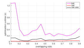
(a) Runtime—Bunny.

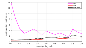
(b) Runtime—Armadillo.

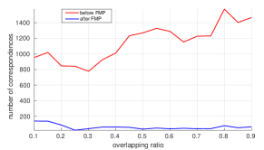
(c) Number of matches before and after FMP—Bunny.

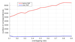
(d) Number of matches before and after FMP—Armadillo.

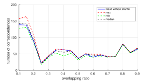
(e) Statistics of $|\mathcal{C^{\prime}}|$ in 100 runs of FMP with shuffled data processing order—Bunny.

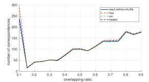
(f) Statistics of $|\mathcal{C^{\prime}}|$ in 100 runs of FMP with shuffled data processing order—Armadillo.

Figure 6: The effect of FMP on data with varied overlapping ratios $\tau$. The runtime of only FMP was reported to show the portion of runtime in FMP + BnB spending on FMP.

Data	Bunny					Armadillo
$\tau$	$|\mathbf{P}|$	$|\mathbf{Q}|$	$|\mathbf{P}_{key}|$	$|\mathbf{Q}_{key}|$	$|\mathcal{C}|$	$|\mathbf{P}|$	$|\mathbf{Q}|$	$|\mathbf{P}_{key}|$	$|\mathbf{Q}_{key}|$	$|\mathcal{C}|$
0.10	15499	15499	233	140	954	77927	77927	1410	820	5097
0.15	15918	15918	248	139	1019	80033	80033	1478	863	5369
0.20	16360	16360	257	147	846	82256	82256	1554	922	5846
0.25	16827	16827	266	153	842	84606	84606	1613	967	6185
0.30	17322	17322	276	155	778	87095	87095	1676	981	6010
0.35	17847	17847	290	160	924	89734	89734	1745	1045	6558
0.40	18405	18405	298	173	1011	92538	92538	1809	1083	6744
0.45	18999	18999	307	170	1233	95524	95524	1862	1136	7000
0.50	19632	19632	321	175	1270	98708	98708	1923	1140	7417
0.55	20309	20309	332	182	1328	102111	102111	1969	1198	7472
0.60	21034	21034	340	190	1289	105758	105758	2033	1216	7725
0.65	21813	21813	348	193	1153	109675	109675	2053	1284	7957
0.70	22652	22652	380	200	1227	113894	113894	2114	1284	7953
0.75	23558	23558	390	205	1231	118449	118449	2160	1360	8444
0.80	24540	24540	400	221	1574	123385	123385	2253	1407	8741
0.85	25607	25607	413	228	1404	128749	128749	2297	1441	8706
0.90	26771	26771	426	227	1466	134602	134602	2352	1475	8664

Table 1: Size of the controlled data. $|\mathbf{P}|$ and $|\mathbf{Q}|$: size of the input point clouds. $|\mathbf{P}_{key}|$ and $|\mathbf{Q}_{key}|$: number of keypoints.

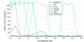
(a) Rotation error—Bunny.

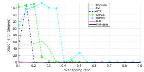
(b) Rotation error—Armadillo.

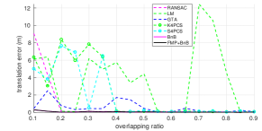
(c) Translation error—Bunny.

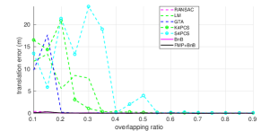
(d) Translation error—Armadillo.

Figure 7: The registration accuracy of all methods on data with varied overlapping ratios $\tau$.

6.1 Controlled data

To refer to our fast match pruning step (Algorithm 3), we abbreviate it as FMP in the rest of this paper. We first show the effect of FMP to the speed of our method, by comparing

• FMP + BnB: Algorithm 2 with FMP for preprocessing;

• BnB: Algorithm 2 without preprocessing;

• FMP: Algorithm 3;

on data with varied overlap ratios $\tau$. Varying $\tau$ showed the performance for different outlier rates. And to preserve the effect of feature matching, we chose to manipulate $\tau$ instead of the outlier rate directly. $\tau$ was controlled by sampling two subsets from a complete point cloud (Bunny and Armadillo in this experiment). Each subset contains $\lfloor\frac{2}{4-2\tau}\rfloor$ of all points, and the second subset is displaced relative to the first one with a randomly generated 4DOF transformation. (3D translation and rotation around the vertical). Moreover, the point clouds are rescaled to have an average point-to-point distance of 0.05 m, and contaminated with uniform random noise of magnitude $[0\ldots 0.05]$ m.

Given two point clouds, the initial match set $\mathcal{C}$ was generated (here and in all subsequent experiments) by

1. Voxel Grid (Lee et al., 2001) down-sampling and ISS (Zhong, 2009) keypoint extraction;

2. FPFH feature (Rusu et al., 2009) computation and matching on keypoints. $\mathbf{p}_{i}$ and $\mathbf{q}_{i}$ were selected into $\mathcal{C}$ if their FPFH features are one of the $\lambda$ nearest neighbours to each other. Empirically, $\lambda$ needs to be a bit larger than 1 to generate enough inliers. We set $\lambda=10$ in all experiments.

The inlier threshold $\epsilon$ was set to 0.05 m according to the noise level.

Figure 6 reports the runtime of the three algorithms and the number of matches before and after FMP, with $\tau$ varied from 0.1 to 0.9. See Table 1 for the input size. As shown in Figure 6(a) and 6(b), due to the extremely high outlier rate, BnB was much slower when $\tau$ is small, whereas FMP + BnB remained efficient for all $\tau$. This significant acceleration came from the drastically reduced input size (more than 90% of the outliers were pruned) after executing FMP (Figure 6(c) and 6(d)), and the extremely low overhead of FMP.

Note that the data storing order of $\mathcal{C}$ was used as the data processing order (the order of $k$ in the for-loop of Algorithm 3) in FMP for all registration tasks in this paper. Though theoretically the data processing order of FMP does affect the size $|\mathcal{C}^{\prime}|$ of the pruned match set, in practice, this effect is minor. To show the stability of FMP under different data processing orders, we executed FMP 100 times given the same input match set, but with randomly shuffled data processing order in each FMP execution. Figures 6(e) and 6(f) report the median, minimum and maximum value of $|\mathcal{C^{\prime}}|$ in 100 runs, and the value of $|\mathcal{C^{\prime}}|$ using the original data storing order as the data processing order. As can be seen, the value $|\mathcal{C^{\prime}}|$ is stable across all instances.

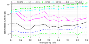
(a) Runtime for optimization—Bunny.

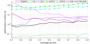
(b) Runtime for optimization—Armadillo.

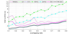
(c) Total runtime—Bunny.

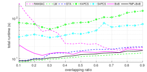
(d) Total runtime—Armadillo.

Figure 8: The log scaled runtime of all methods with (up) and without (bottom) input genreration (only generating keypoints for K4PCS and S4PCS) on controlled data.

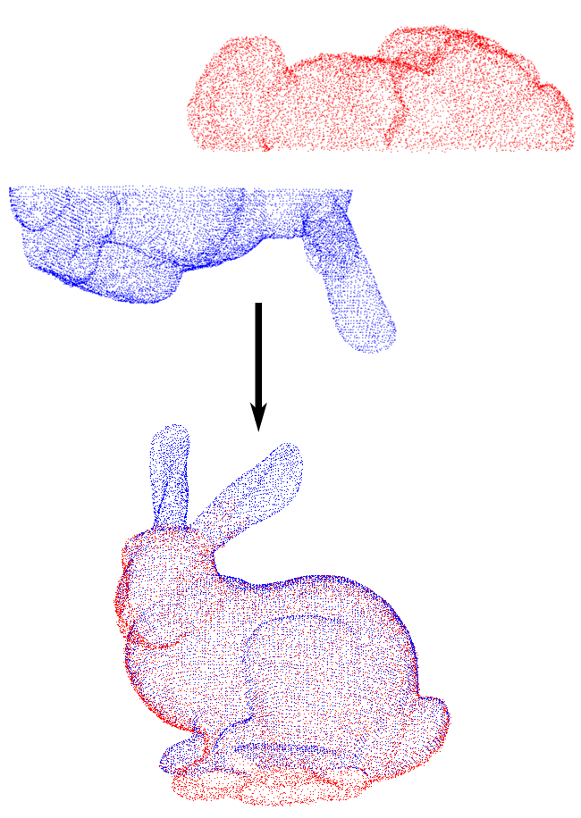
(a) Bunny.

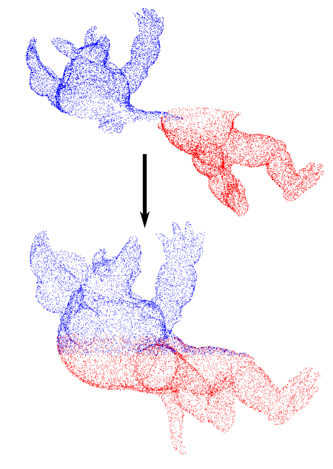
(b) Armadillo.

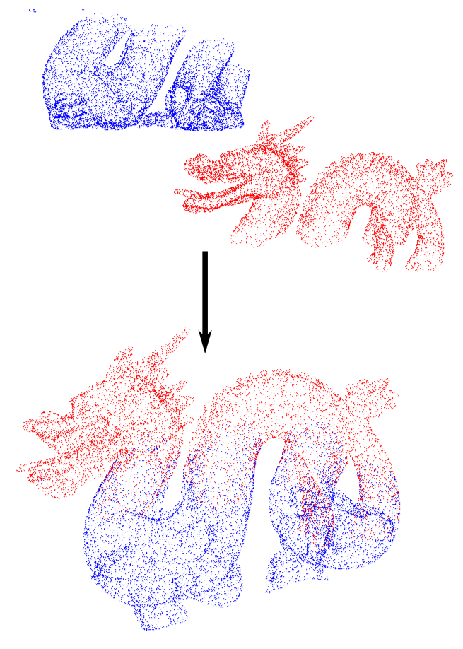
(c) Dragon.

Figure 9: Registered controlled data ($\tau=0.1$). 10k points are shown for each point cloud.

To show the advantage of our method, we also compared it against the following state-of-the-art approaches, on the same set of data.

• 4DOF RANSAC (Fischler and Bolles, 1981), using 2-point samples for 4DOF pose estimation,and with the probability of finding a valid sample set to 0.99;

• 4DOF version of the lifting method (LM) (Zhou et al., 2016), a match-based robust optimization approach. The annealing rate was tuned to 1.1 for the best performance;

• The Game-Theory approach (GTA) (Albarelli et al., 2010), a fast outlier removal method;

• Super 4PCS (S4PCS) (Mellado et al., 2014), a fast 4PCS (Aiger et al., 2008) variant.

• Keypoint-based 4PCS (K4PCS) (Theiler et al., 2014), which applies 4PCS to keypoints.

The first three approaches are match-based and the last two operates on raw point sets (ISS keypoints were used here). The 4DOF version of RANSAC and LM were used for a fair comparison, since they had similar accuracy but were much faster than their 6DOF counterparts. We note that, when working with levelled point clouds, the translation alone must already align the $z$-coordinates of two points up to the inlier threshold $\epsilon$. This can be checked before sampling/applying the rotation. Where applicable, we use this trick to save computations (for all methods). For GTA as well as 4PCS variants, the original versions for 6DOF had to be used, since it is not obvious how to constrain the underlying algorithms to 4DOF.

Figure 7 shows the accuracy of all methods, which was measured as the difference between the estimated transformation and the known ground truth. As expected, BnB and FMP + BnB returned high quality solutions for all setups. In contrast, due to the lack of optimality guarantees, other methods performed badly when $\tau$ was small. Meanwhile, Figure 8 shows both the runtime including and not including the input generation (keypoint extraction and/or feature matching). FMP + BnB was faster than most of its competitors. Note that most of the total runtime was spent on input generation. Other than sometimes claimed, exact optimization is not necessarily slow and does in fact not create a computational bottleneck for registration. Figure 9 shows some visual examples of point clouds aligned with our method.

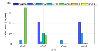
(a) Rotation error—Arch.

(b) Rotation error—Facility.

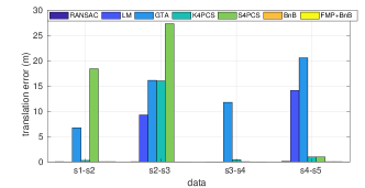
(c) Translation error—Arch.

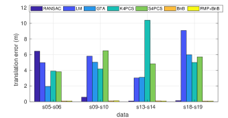
(d) Translation error—Facility.

Figure 10: The accuracy of all registration methods on real-world data.

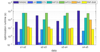
(a) Runtime for optimization—Arch.

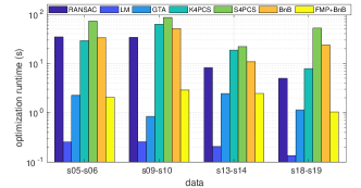
(b) Runtime for optimization—Facility.

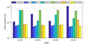
(c) Total runtime—Arch.

(d) Total runtime—Facility.

Figure 11: The log scaled runtime of all methods with (up) and without (bottom) input genreration (only generating keypoints for K4PCS and S4PCS) on real-world data.

6.2 Challenging real-world data

Arch
Data	$|\mathbf{P}|$	$|\mathbf{Q}|$	$|\mathbf{P}_{key}|$	$|\mathbf{Q}_{key}|$	$|\mathcal{C}|$
s01-s02	23561732	30898999	7906	4783	19879
s02-s03	30898999	25249235	4783	7147	19344
s03-s04	25249235	29448437	7147	5337	22213
s04-s05	29448437	27955953	5337	4676	15529

Facility
Data	$|\mathbf{P}|$	$|\mathbf{Q}|$	$|\mathbf{P}_{key}|$	$|\mathbf{Q}_{key}|$	$|\mathcal{C}|$
s05-s06	10763194	10675580	2418	2727	10679
s09-s10	10745525	10627814	2960	1327	7037
s12-s13	10711291	10441772	1227	2247	6001
s18-s19	10541274	10602884	1535	2208	7260

Table 2: Size of the real-world data. $|\mathbf{P}_{key}|$ and $|\mathbf{Q}_{key}|$: number of keypoints.

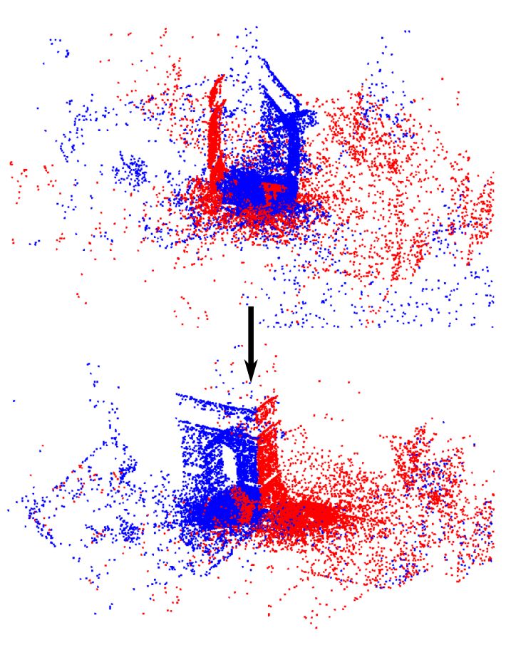
(a) s3-s4—Arch.

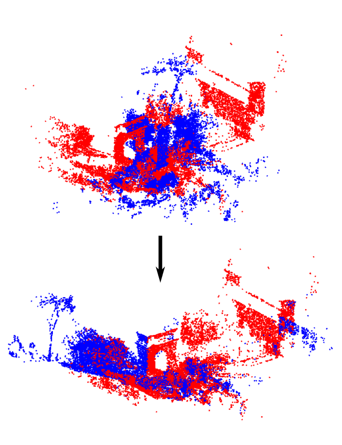
(b) s4-s5—Arch.

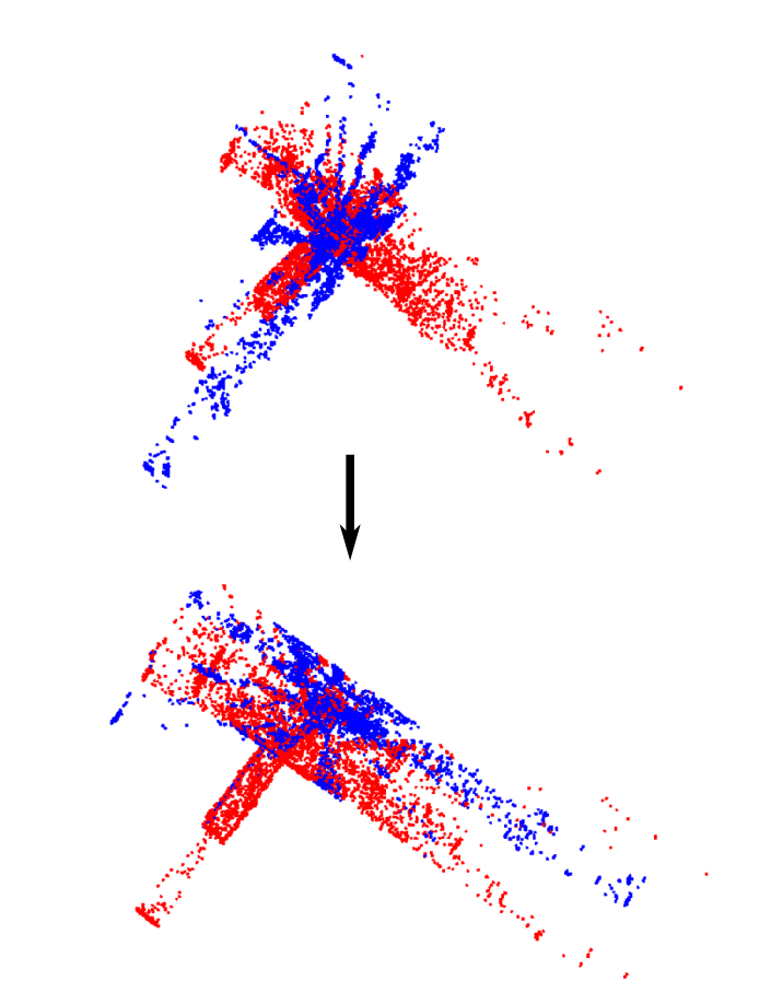
(c) s9-s10—Facility.

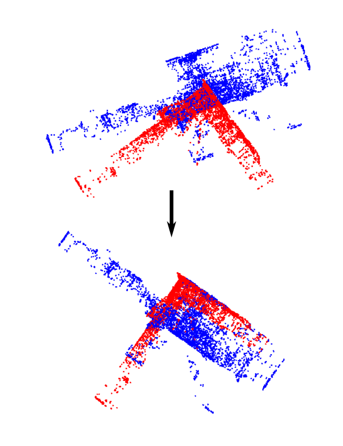
(d) s18-s19—Facility.

Figure 12: Registered pairwise real-world data. 10k points are shown for each point cloud.

To demonstrate the practicality of our method, comparisons on large sale LiDAR datasets were also performed. Figure 10 reports the accuracy of all methods on an outdoor dataset, Arch, and an indoor dataset, Facility. Among the datasets used in  (Theiler et al., 2015), these are the most challenging ones, which most clearly demonstrate the advantages of our proposed method. We point out that both are not staged, but taken from real surveying projects and representative for the registration problems that arise in difficult field campaigns. For completeness, Appendix 9.3 contains results on easier data, where most of the compared methods work well). The accuracy was again measured by the difference between the estimated and ground truth (provided in the selected datasets, see (Theiler et al., 2015) for details) relative poses. Similar as before, at a reasonable error threshold of $15$ cm for translation, respectively $1^{\circ}$ for rotation, our method had 100% success rate; whereas failure cases occurred with all other methods. And as shown in Figure 11, FMP + BnB showed comparable speed than its competitors on all data. It successfully registered millions of points and tens of thousands of point matches (see Table 2) within 100 s, including the match generation time. We see the excellent balance between high accuracy and reliability on the one hand, and low computation time on the other hand as a particular strength of our method.

Figures 12–15 visually show various large scale scenes (pair-wise and complete) registered by our method; more detailed demonstrations can be found in the video demo in our project homepage. Note that the runtime for registering a complete dataset (in Figure 3 and 17 to 19) was slightly less than the sum of pair-wise runtimes, since a scan forms part of multiple pairs, but keypoints and FPFH features need to be extracted only once and can then be reused.

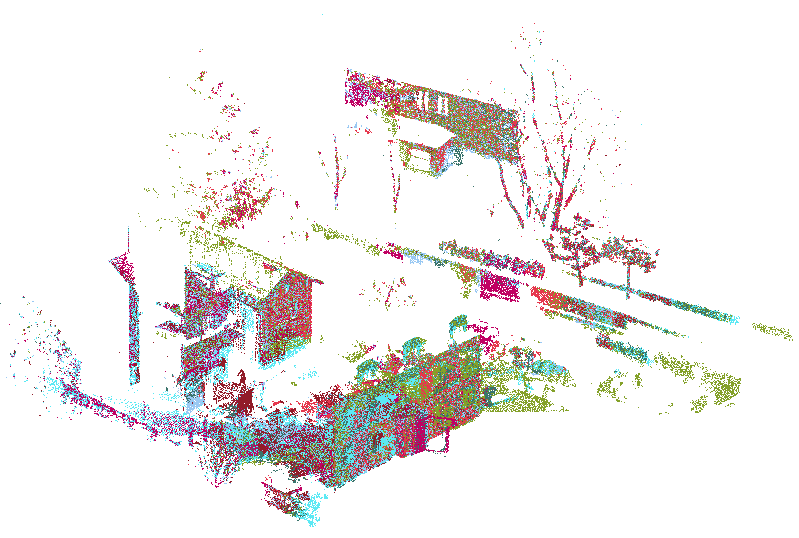
Figure 13: Complete registration result—Facade. All 7 scans were registered in 134.95s.

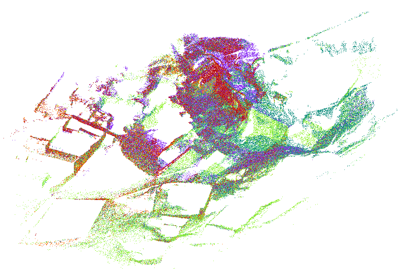
Figure 14: Complete registration result—Courtyard. All 8 scans were registered in 84.02s.

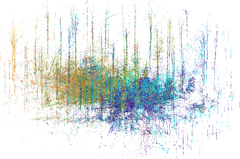
Figure 15: Complete registration result—Trees. All 6 scans were registered in 142.72s.

7 Conclusion

We have described a practical and optimal solution for terrestrial LiDAR scan registration. The main characteristic of our approach is that it combines a reliable, optimal solver with high computational efficiency, by exploiting two properties of terrestrial LiDAR: (1) it restricts the registration problem to 4DOF (3D translation + azimuth), since modern laser scanners have built-in level compensators. And (2) it aggressively prunes the number of matches used to compute the transformation, realising that the sensor noise level is low, therefore a small set of corresponding points is sufficient for accurate registration, so long as they are correct. Given some set of candidate correspondences that may be contaminated with a large number of incorrect matches (which is often the case for real 3D point clouds); our algorithm first applies a fast pruning method that leaves the optimum of the alignment objective unchanged, then uses the reduced point set to find that optimum with the branch-and-bound method. The pruning greatly accelerates the solver while keeping intact the optimality w.r.t. the original problem. The BnB solver explicitly searches the 3D translation space, which can be bounded efficiently; while solving for 1D rotation implicitly with a novel, polynomial-time algorithm. Experiments show that our algorithm is significantly more reliable than previous methods, with competitive speed.

8 Acknowledgement

This work was supported by the ARC grant DP160103490.

9 Appendix

9.1 Compute $\mathtt{int}_{i}$ and solve the max-stabbing problem

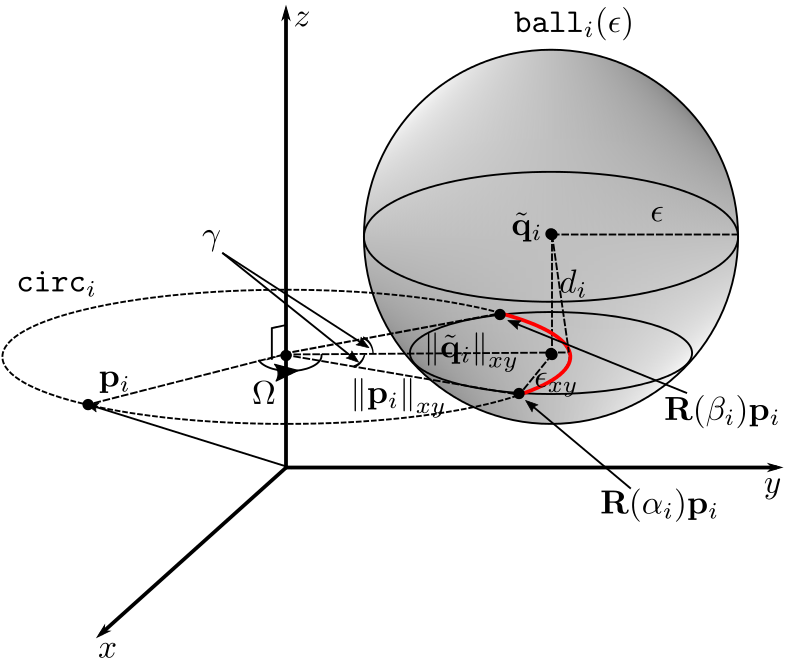
Figure 16: Illustration of Algorithm 4, $\mathtt{int}_{i}$ is rendered in red.

Algorithm 4 Compute the angle interval that aligns $\mathbf{p}_{i}$ with $\tilde{\mathbf{q}}_{i}$

0:  $\mathbf{p}_{i}$, $\tilde{\mathbf{q}}_{i}$ and $\epsilon$, such that $d_{i}\leq\epsilon$.

1:  $\epsilon_{xy}\leftarrow\sqrt{\epsilon^{2}-(\mathbf{p}_{i}(3)-\tilde{\mathbf{q}}_{i}(3))^{2}}$

2:  if $|\lVert\mathbf{p}_{i}\rVert_{xy}+\lVert\tilde{\mathbf{q}}_{i}\rVert_{xy}|\leq\epsilon_{xy}$ then

3:     return  $[0,2\pi]$.

4:  else

5:     $\Omega=azi(\tilde{\mathbf{q}}_{i})-azi(\mathbf{p}_{i}),\gamma=\arccos{\frac{\lVert\mathbf{p}_{i}\rVert^{2}_{xy}+\lVert\tilde{\mathbf{q}}_{i}\rVert^{2}_{xy}-\epsilon_{xy}}{2\lVert\mathbf{p}_{i}\rVert_{xy}\lVert\tilde{\mathbf{q}}_{i}\rVert_{xy}}}$.

6:     return  $[\Omega-\gamma,\Omega+\gamma]$.

7:  end if

Algorithm 4 shows how to compute $\mathtt{int}_{i}=[\alpha_{i},\beta_{i}]$ for each $(\mathbf{p}_{i},\tilde{\mathbf{q}}_{i})$ during rotation search. As shown in Figure 16, $\mathtt{circ}_{i}$ and $\mathtt{ball}_{i}(\epsilon)$ intersect if and only if the closest distance $d_{i}$ from $\tilde{\mathbf{q}}_{i}$ to $\mathtt{circ}_{i}$ is within $\epsilon$, where

$$d_{i}=\sqrt{(\lVert\mathbf{p}_{i}\rVert_{xy}-\lVert\tilde{\mathbf{q}}_{i}\rVert_{xy})^{2}+(\mathbf{p}_{i}(3)-\tilde{\mathbf{q}}_{i}(3))^{2}}.$$ (28)

In the above equation, $\mathbf{p}_{i}(3)$ is the 3rd channel of $\mathbf{p}_{i}$ and $\lVert\mathbf{p}_{i}\rVert_{xy}=\sqrt{\mathbf{p}_{i}(1)^{2}+\mathbf{p}_{i}(2)^{2}}$ is the horizontal length of $\mathbf{p}_{i}$. And the two intersecting points of $\mathtt{circ}_{i}$ and $\mathtt{ball}_{i}(\epsilon)$, namely $\mathbf{R}(\alpha_{i})\mathbf{p}_{i}$ and $\mathbf{R}(\beta_{i})\mathbf{p}_{i}$, have the same azimuthal angular distance $\gamma$ to $\tilde{\mathbf{q}}_{i}$. And by computing the azimuth $\Omega$ from $\mathbf{p}_{i}$ to $\tilde{\mathbf{q}}_{i}$, i.e., $\Omega=azi(\tilde{\mathbf{q}}_{i})-azi(\mathbf{p}_{i})$, where $azi(\cdot)$ is the azimuth of a point, $\mathtt{int}_{i}$ is simply $[\Omega-\gamma,\Omega+\gamma]$. Note that when $\mathtt{circ}_{i}$ is inside $\mathtt{ball}_{i}(\epsilon)$ (Line 2), $\mathtt{int}_{i}$ is $[0,2\pi]$.

$\gamma$ is computed by the law of cosines, because it is an interior angle of the triangle whose three edge lengths are $\lVert\mathbf{p}_{i}\rVert_{xy}$, $\lVert\tilde{\mathbf{q}}_{i}\rVert_{xy}$ and $\epsilon_{xy}$, where $\epsilon_{xy}$ is the horizontal distance between $\tilde{\mathbf{q}}_{i}$ and $\mathbf{R}(\alpha_{i})\mathbf{p}_{i}$ (or $\mathbf{R}(\beta_{i})\mathbf{p}_{i}$).

Algorithm 5 Max-Stabbing algorithm for 1D rotation estimation

0:  $U=\{\mathtt{int}_{i}\}_{i=1}^{M}$, where $\mathtt{int}_{i}=[\alpha_{i},\beta_{i}]$.

1:  $\mathbf{V}\leftarrow\bigcup\limits_{i=1}^{M}\{[\alpha_{i},0],[\beta_{i},1]\}$, sort $\mathbf{V}$ ascendingly according to a1: and a2:.

2:  $\tilde{\delta}\leftarrow 0$, $\delta\leftarrow 0$.

3:  for each $\mathbf{v}\in\mathbf{V}$ do

4:     if $\mathbf{v}(2)=0$ then

5:        $\delta\leftarrow\delta+1$. And if $\delta>\tilde{\delta}$, then $\tilde{\delta}\leftarrow\delta,\tilde{\theta}\leftarrow\mathbf{v}(1)$.

6:     else

7:        $\delta\leftarrow\delta-1$.

8:     end if

9:  end for

10:  return  $\tilde{\delta},\tilde{\theta}$.

After computing all $\mathtt{int}_{i}$’s, the max-stabbing problem (11) can be efficiently solved by Algorithm 5. Observe that one of the endpoints among all $\mathtt{int}_{i}$’s must achieve the max-stabbing, the idea of Algorithm 5 is to compute the stabbing value $\delta$ for all endpoints and find the maximum one.

We first pack all endpoints into an array $\mathbf{V}=\bigcup\limits_{i=1}^{M}\{[\alpha_{i},0],[\beta_{i},1]\}$. The $0/1$ label attached to each endpoint represents whether it is the end of an $\mathtt{int}_{i}$, i.e., $\beta_{i}$. Then, to efficiently compute each $\delta$, we sort $\mathbf{V}$ so that the endpoints with

1. smaller angles;

2. and the same angle but are the start of an $\mathtt{int}_{i}$ (the assigned label is 0);

are moved to the front. After sorting, we initialize $\delta$ to 0 and traverse $\mathbf{V}$ from the first element to the last. When we “hit” the beginning of an $\mathtt{int}_{i}$, we increment $\delta$ by 1, and when we “hit” the end of an $\mathtt{int}_{i}$, $\delta$ is reduced by 1. The max-stabbing value $\tilde{\delta}$ and its corresponding angle $\tilde{\theta}$ are returned in the end.

Since the time complexity for sorting and traversing $\mathbf{V}$ is respectively $\mathcal{O}(M\log M)$ and $\mathcal{O}(M)$, the one for Algorithm 5 is $\mathcal{O}(M\log M)$. The space complexity of $\mathcal{O}(M)$ can be achieved with advanced sorting algorithms like merge sort.

9.2 Proof of Lemma 1

First, to prove (15), we re-express $\mathbf{t}^{*}(\mathbb{S})=\underset{\mathbf{t}\in\mathbb{S}}{\operatorname*{arg\,max}}~{}U(\mathbf{t}\mid\mathcal{C},\epsilon)$ as $\mathbf{t}_{\mathbb{S}}+\mathbf{t}^{*}{{}^{\prime}}(\mathbb{S})$, where $\lVert\mathbf{t}^{*}{{}^{\prime}}(\mathbb{S})\rVert\leq d_{\mathbb{S}}$. Using this re-expression, we have

$$\lVert\mathbf{R}(\theta)\mathbf{p}_{i}+\mathbf{t}_{\mathbb{S}}+\mathbf{t}^{*}{{}^{\prime}}(\mathbb{S})-\mathbf{q}_{i}\rVert\leq\epsilon$$ (29a)

$$\Rightarrow \lVert\mathbf{R}(\theta)\mathbf{p}_{i}+\mathbf{t}_{\mathbb{S}}-\mathbf{q}_{i}\rVert-\lVert\mathbf{t}^{*}{{}^{\prime}}(\mathbb{S})\rVert\leq\epsilon$$ (29b)

$$\Rightarrow \lVert\mathbf{R}(\theta)\mathbf{p}_{i}+\mathbf{t}_{\mathbb{S}}-\mathbf{q}_{i}\rVert-d_{\mathbb{S}}\leq\epsilon$$ (29c)

$$\Leftrightarrow \lVert\mathbf{R}(\theta)\mathbf{p}_{i}+\mathbf{t}_{\mathbb{S}}-\mathbf{q}_{i}\rVert\leq\epsilon+d_{\mathbb{S}}.$$ (29d)

(29a) to (29b) is due to the triangle inequality. According to (29a) and (29d), as long as $(\mathbf{p}_{i},\mathbf{q}_{i})$ contributes 1 in $\underset{\mathbf{t}\in\mathbb{S}}{\max}~{}U(\mathbf{t}\mid\mathcal{C},\epsilon)=U(\mathbf{t}_{\mathbb{S}}+\mathbf{t}^{*}{{}^{\prime}}(\mathbb{S})\mid\mathcal{C},\epsilon)$, it must also contribute 1 in $U(\mathbf{t}_{\mathbb{S}}\mid\mathcal{C},\epsilon+d_{\mathbb{S}})$, i.e., $U(\mathbf{t}_{\mathbb{S}}\mid\mathcal{C},\epsilon+d_{\mathbb{S}})\geq\underset{\mathbf{t}\in\mathbb{S}}{\max}~{}U(\mathbf{t}\mid\mathcal{C},\epsilon)$.

And when $\mathbb{S}$ tends to a point $\mathbf{t}$, $d_{\mathbb{S}}$ tends to 0. Therefore, $\bar{U}(\mathbb{S}\mid\mathcal{C},\epsilon)=U(\mathbf{t}_{\mathbb{S}}\mid\mathcal{C},\epsilon+d_{\mathbb{S}})\rightarrow U(\mathbf{t}\mid\mathcal{C},\epsilon)$.

9.3 Further results

Figure 17 to 19 show the accuracy and runtime of our method and all other competitors in Section 6.2 for Facade, Courtyard and Trees. The inlier threshold $\epsilon$ were set to 0.05 m for Facade, 0.2 m for Courtyard and 0.2 m for Trees.

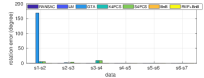
(a) Rotation error.

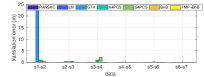
(b) Translation error.

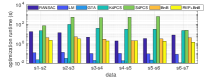
(c) Runtime for optimization.

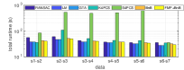
(d) Total runtime.

Figure 17: Accuracy and log scaled runtime for Facade.

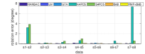
(a) Rotation error.

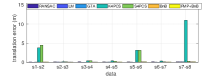
(b) Translation error.

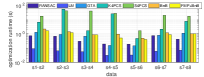
(c) Runtime for optimization.

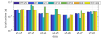
(d) Total runtime.

Figure 18: Accuracy and log scaled runtime for Courtyard.

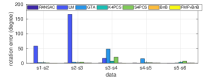
(a) Rotation error.

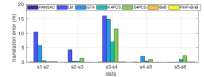
(b) Translation error.

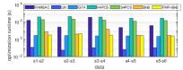
(c) Runtime for optimization.

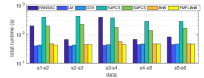
(d) Total runtime.

Figure 19: Accuracy and log scaled runtime for Trees.

References

- Aiger et al. (2008) Aiger, D., Mitra, N. J., Cohen-Or, D., 2008. 4-points congruent sets for robust pairwise surface registration. In: ACM Transactions on Graphics (TOG). Vol. 27. ACM, p. 85.
- Akca (2003) Akca, D., 2003. Full automatic registration of laser scanner point clouds. Tech. rep., ETH Zurich.
- Albarelli et al. (2010) Albarelli, A., Rodola, E., Torsello, A., 2010. A game-theoretic approach to fine surface registration without initial motion estimation. In: Computer Vision and Pattern Recognition (CVPR), 2010 IEEE Conference on. IEEE, pp. 430–437.
- Bazin et al. (2012) Bazin, J.-C., Seo, Y., Pollefeys, M., 2012. Globally optimal consensus set maximization through rotation search. In: Asian Conference on Computer Vision. Springer, pp. 539–551.
- Besl and McKay (1992) Besl, P. J., McKay, N. D., 1992. Method for registration of 3-d shapes. In: Sensor Fusion IV: Control Paradigms and Data Structures. Vol. 1611. International Society for Optics and Photonics, pp. 586–607.
- Brenner and Dold (2007) Brenner, C., Dold, C., 2007. Automatic relative orientation of terrestrial laser scans using planar structures and angle constraints. In: ISPRS Workshop on Laser Scanning. Vol. 200. pp. 84–89.
- Breuel (2001) Breuel, T. M., 2001. A practical, globally optimal algorithm for geometric matching under uncertainty. Electronic Notes in Theoretical Computer Science 46, 188–202.
- Bustos and Chin (2017) Bustos, A. P., Chin, T.-J., 2017. Guaranteed outlier removal for point cloud registration with correspondences. IEEE Transactions on Pattern Analysis and Machine Intelligence.
- Campbell and Petersson (2016) Campbell, D., Petersson, L., 2016. Gogma: Globally-optimal gaussian mixture alignment. In: CVPR. pp. 5685–5694.
- Chen et al. (1999) Chen, C.-S., Hung, Y.-P., Cheng, J.-B., 1999. Ransac-based darces: A new approach to fast automatic registration of partially overlapping range images. IEEE Transactions on Pattern Analysis and Machine Intelligence 21 (11), 1229–1234.
- Chin et al. (2018) Chin, T.-J., Cai, Z., Neumann, F., 2018. Robust fitting in computer vision: Easy or hard? arXiv preprint arXiv:1802.06464.
- Chin and Suter (2017) Chin, T.-J., Suter, D., 2017. The maximum consensus problem: Recent algorithmic advances. Synthesis Lectures on Computer Vision 7 (2), 1–194.
- De Berg et al. (2000) De Berg, M., Van Kreveld, M., Overmars, M., Schwarzkopf, O. C., 2000. Computational geometry. In: Computational geometry. Springer, pp. 1–17.
- Drost et al. (2010) Drost, B., Ulrich, M., Navab, N., Ilic, S., 2010. Model globally, match locally: Efficient and robust 3d object recognition. In: Computer Vision and Pattern Recognition (CVPR), 2010 IEEE Conference on. Ieee, pp. 998–1005.
- Fischler and Bolles (1981) Fischler, M. A., Bolles, R. C., 1981. Random sample consensus: a paradigm for model fitting with applications to image analysis and automated cartography. Communications of the ACM 24 (6), 381–395.
- Franaszek et al. (2009) Franaszek, M., Cheok, G. S., Witzgall, C., 2009. Fast automatic registration of range images from 3d imaging systems using sphere targets. Automation in Construction 18 (3), 265–274.
- Głomb (2009) Głomb, P., 2009. Detection of interest points on 3d data: Extending the harris operator. In: Computer Recognition Systems 3. Springer, pp. 103–111.
- Harris and Stephens (1988) Harris, C., Stephens, M., 1988. A combined corner and edge detector. In: Alvey vision conference. Vol. 15. Citeseer, pp. 10–5244.
- Houshiar et al. (2015) Houshiar, H., Elseberg, J., Borrmann, D., Nüchter, A., 2015. A study of projections for key point based registration of panoramic terrestrial 3d laser scan. Geo-spatial Information Science 18 (1), 11–31.
- Lee et al. (2001) Lee, K., Woo, H., Suk, T., 2001. Data reduction methods for reverse engineering. The International Journal of Advanced Manufacturing Technology 17 (10), 735–743.
- Lowe (1999) Lowe, D. G., 1999. Object recognition from local scale-invariant features. In: Computer vision, 1999. The proceedings of the seventh IEEE international conference on. Vol. 2. Ieee, pp. 1150–1157.
- Lu and Milios (1997) Lu, F., Milios, E., 1997. Globally consistent range scan alignment for environment mapping. Autonomous robots 4 (4), 333–349.
- Mellado et al. (2014) Mellado, N., Aiger, D., Mitra, N. J., 2014. Super 4pcs fast global pointcloud registration via smart indexing. In: Computer Graphics Forum. Vol. 33. Wiley Online Library, pp. 205–215.
- Parra Bustos and Chin (2015) Parra Bustos, A., Chin, T.-J., 2015. Guaranteed outlier removal for rotation search. In: Proceedings of the IEEE International Conference on Computer Vision. pp. 2165–2173.
- Parra Bustos et al. (2016) Parra Bustos, A., Chin, T.-J., Eriksson, A., Li, H., Suter, D., 2016. Fast rotation search with stereographic projections for 3d registration. IEEE Transactions on Pattern Analysis and Machine Intelligence 38 (11), 2227–2240.
- Pomerleau et al. (2013) Pomerleau, F., Colas, F., Siegwart, R., Magnenat, S., 2013. Comparing icp variants on real-world data sets. Autonomous Robots 34 (3), 133–148.
- Rabbani et al. (2007) Rabbani, T., Dijkman, S., van den Heuvel, F., Vosselman, G., 2007. An integrated approach for modelling and global registration of point clouds. ISPRS journal of Photogrammetry and Remote Sensing 61 (6), 355–370.
- Rusinkiewicz and Levoy (2001) Rusinkiewicz, S., Levoy, M., 2001. Efficient variants of the icp algorithm. In: 3-D Digital Imaging and Modeling, 2001. Proceedings. Third International Conference on. IEEE, pp. 145–152.
- Rusu et al. (2009) Rusu, R. B., Blodow, N., Beetz, M., 2009. Fast point feature histograms (fpfh) for 3d registration. In: Robotics and Automation, 2009. ICRA’09. IEEE International Conference on. IEEE, pp. 3212–3217.
- Rusu et al. (2008) Rusu, R. B., Blodow, N., Marton, Z. C., Beetz, M., 2008. Aligning point cloud views using persistent feature histograms. In: Intelligent Robots and Systems, 2008. IROS 2008. IEEE/RSJ International Conference on. IEEE, pp. 3384–3391.
- Scovanner et al. (2007) Scovanner, P., Ali, S., Shah, M., 2007. A 3-dimensional sift descriptor and its application to action recognition. In: Proceedings of the 15th ACM international conference on Multimedia. ACM, pp. 357–360.
- Svarm et al. (2014) Svarm, L., Enqvist, O., Oskarsson, M., Kahl, F., 2014. Accurate localization and pose estimation for large 3d models. In: Proceedings of the IEEE Conference on Computer Vision and Pattern Recognition. pp. 532–539.
- Theiler et al. (2014) Theiler, P. W., Wegner, J. D., Schindler, K., 2014. Keypoint-based 4-points congruent sets–automated marker-less registration of laser scans. ISPRS journal of photogrammetry and remote sensing 96, 149–163.
- Theiler et al. (2015) Theiler, P. W., Wegner, J. D., Schindler, K., 2015. Globally consistent registration of terrestrial laser scans via graph optimization. ISPRS Journal of Photogrammetry and Remote Sensing 109, 126–138.
- Turk and Levoy (1994) Turk, G., Levoy, M., 1994. Zippered polygon meshes from range images. In: Proceedings of the 21st annual conference on Computer graphics and interactive techniques. ACM, pp. 311–318.
- Yang et al. (2016) Yang, J., Li, H., Campbell, D., Jia, Y., 2016. Go-icp: a globally optimal solution to 3d icp point-set registration. IEEE transactions on pattern analysis and machine intelligence 38 (11), 2241–2254.
- Yu and Ju (2018) Yu, C., Ju, D. Y., 2018. A maximum feasible subsystem for globally optimal 3d point cloud registration. Sensors 18 (2), 544.
- Zhong (2009) Zhong, Y., 2009. Intrinsic shape signatures: A shape descriptor for 3d object recognition. In: Computer Vision Workshops (ICCV Workshops), 2009 IEEE 12th International Conference on. IEEE, pp. 689–696.
- Zhou et al. (2016) Zhou, Q.-Y., Park, J., Koltun, V., 2016. Fast global registration. In: European Conference on Computer Vision. Springer, pp. 766–782.