A relaxation time model for efficient and accurate prediction of lattice thermal conductivity

Abstract

Prediction of lattice thermal conductivity is important to many applications and technologies, especially for high-throughput materials screening. However, the state-of-the-art method based on three-phonon scattering process is bound with high computational cost while semi-empirical models such as the Slack equation are less accurate. In this work, we examined the theoretical background of the commonly-used computational models for high-throughput thermal conductivity prediction and proposed an efficient and accurate method based on an approximation for three-phonon scattering strength. This quasi-harmonic approximation has comparable computational cost with many widely-used thermal conductivity models but had the best performance in regard to quantitative accuracy. As compared to many models that can only predict lattice thermal conductivity values, this model also allows to include Normal processes and obtain the phonon relaxation time.

I Introduction

Lattice thermal conductivity is an important material property that plays a key role in many applications and technologies Cahill et al. (2002, 2014). For example, heat generation has become a serious issue to further improve the performance of semiconductor devices, and thus materials with high thermal conductivity are desired for heat dissipation Cahill et al. (2002); Garimella et al. (2012); Lindsay et al. (2013a). While in thermoelectric applications, materials with low thermal conductivity are more favorable since the thermoelectric performance is inversely proportional to thermal conductivity Qiu et al. (2012); Yang et al. (2014); Gorai et al. (2016). Therefore, finding an efficient and robust method to predict lattice thermal conductivity is a desirable goal in itself van Roekeghem et al. (2016); Nath et al. (2017). With a high-throughput computational framework established, it will be much more efficient to search and design new materials with tailored thermal conductivities, since we can do materials characterization and selection based on theoretical understanding before the trial-and-error experimental procedures White Paper (2011).

Nevertheless, developing a both accurate and also computationally inexpensive method remains a big challenge Nath et al. (2017); Plata et al. (2017): accurate methods are bound with high computational costs, and fast methods often lack the quantitative accuracy. As far as we know, the state-of-the-art method for predicting lattice thermal conductivity is solving Boltzmann transport equation (BTE) with interatomic force constants (IFCs) calculated from first-principles calculations. The advantage of this method is that it is free of fitting parameters and has a good predictive power Lindsay (2016). However, extracting anharmonic IFCs from first-principles calculations is computationally very expensive. Plata et al. Plata et al. (2017) attempted to solve such a problem by making effective use of crystal symmetries to reduce the number of static first-principles calculations. The computational cost is reduced compared with other packages like ShengBTE Li et al. (2014) and Phono3py Togo et al. (2015) but it must still be quite large because dozens of static first-principles calculations with large supercells are still required. Compared with ShengBTE, Carrete et al. Carrete et al. (2017) developed a similar but more efficient software package named almaBTE but the major concern about computational cost of anharmonic IFCs remains unaddressed.

Besides the aforementioned method, researchers have tried to use some semi-empirical models to predict lattice thermal conductivity with less computational cost. Among them, the Debye-Grüneisen model Blanco et al. (2004) and simplified Debye-Callaway model Miller et al. (2017) require the least computational resource. These two models do not require the computation of harmonic and anharmonic IFCs, and therefore have much less computational cost. However, the Debye-Grüneisen model Blanco et al. (2004) did not show good quantitative accuracy when applied to material data sets with different structures Toher et al. (2014). It has been implemented in the Automatic-GIBBS-Library (AGL) framework in a high-throughput fashion Toher et al. (2014) . And we can find that the Pearson correlation coefficient between the thermal conductivity calculated with AGL and experimental data is high for cubic and rhombohedral structures, but significantly lower for anisotropic materials and half-Heusler compounds Toher et al. (2014). Miller et al. Miller et al. (2017) tried to refine the simplified Debye-Callaway model by introducing four fitting parameters and adding the Grüneisen constant. The fitting parameters are dependent on the chosen material data set and applying such parameters to other materials will be questionable. The quasi-harmonic approximation (QHA) is another family of methods to predict lattice thermal conductivity, which balance between the accuracy and computational cost Nath et al. (2017, 2018). Harmonic IFCs are computed to get more accurate Grüneisen parameters and Debye temperatures with such methods Nath et al. (2017), while the computation of anharmonic IFCs is circumvented. Bjerg et al. Bjerg et al. (2014) introduced a quasi-harmonic model that uses the full dispersion curve computed with harmonic IFCs as the input. The model was derived by comparing the Slack equation and the Klemens-Callaway model for Debye solids Bjerg et al. (2014). Nath et al. Nath et al. (2017) also used the Slack equation to calculate lattice thermal conductivity. They tried different formulations for the two input parameters and found the best combination by comparing their results with experimental values. The computational cost of QHA methods are higher than the Debye-Grüneisen model or simplified Debye-Callaway model but is significantly lower than the full numerical calculation based on BTE. Based on the result by Nath et al. Nath et al. (2017), it can be found that QHA can have better quantitative accuracy than the Debye-Grüneisen model and have less fitting parameters than the simplified Debye-Callaway model. Despite the efforts to refine the semi-empirical models, their physical origins are still unclear, e.g. the phase space Lindsay and Broido (2008) information is contained in none of them. The Slack equation has been widely used in high-throughput computation of lattice thermal conductivity but some approximations used in its original derivation are unnecessary at the present time, including (i) the Debye-like isotropic dispersion relation and (ii) a constant function instead of Dirac delta function used in its derivation.

In this work, we attempt to find a thermal conductivity model that only requires harmonic IFCs as the input, while maintains a good prediction accuracy. We first reviewed the approximations used in deriving those semi-empirical models and tried to identify the necessary approximations at the present time. We proposed a model based on an approximation developed by Leibfried and Schlömann Leibfried and Schlömann (1954); Leibfried (1955), and also Klemens Klemens (1956, 1958) for intrinsic three-phonon scattering strength. This model will use the full phonon dispersion data but do not require anharmonic IFCs as the input, which can greatly reduce the computational cost compared with the full BTE calculation. It has comparable computational cost but better accuracy than existing QHA methods. This model has been compared with Leibfried and Schlömann’s model, the Slack equation, and Slack’s relaxation time model, and further discussed.

II Theoretical background

In order to better understand the physical origins of those semi-empirical models, we first reviewed the development of the theory and the approximations used in their derivation. In semiconductors and insulators, phonons are the major heat carriers and the lattice thermal conductivity $\kappa_{l}$ can be obtained with the following equation Xie et al. (2014, 2016)

$$\kappa_{l}^{\alpha\beta}=\sum_{\lambda}c_{\lambda}v^{\alpha}_{\lambda}v^{\beta}_{\lambda}\tau_{\lambda},$$ (1)

where $\lambda$ denotes different phonon modes that can be distinguished by wave vector $\boldsymbol{q}$ and phonon branch $\nu$. $c_{\lambda}$ is the volumetric heat capacity Turney et al. (2009). $v^{\alpha}_{\lambda}$ and $v^{\beta}_{\lambda}$ are the phonon group velocities in $\alpha$ and $\beta$ directions, respectively. $\tau_{\lambda}$ is the phonon relaxation time. Among these three phonon properties, $c_{\lambda}$ and $\boldsymbol{v}_{\lambda}$ are computationally less expensive than $\tau_{\lambda}$ since they only require harmonic IFCs as the input while computation of $\tau_{\lambda}$ needs both harmonic and anharmonic IFCs. With harmonic IFCs, we can compute phonon frequencies and eigenvectors with harmonic lattice dynamics method Turney et al. (2009). And then $c_{\lambda}$ and $\boldsymbol{v}_{\lambda}$ can be calculated with phonon frequencies as the input. Under single mode relaxation time approximation (SMRTA), the relaxation time can be calculated with Li et al. (2014)

$$\frac{1}{\tau_{\lambda}^{0}}=\sum\limits_{\lambda^{\prime}\lambda^{\prime\prime}}{\left({{\Gamma_{\lambda,\lambda^{\prime},\lambda^{\prime\prime}}^{(+)}}+\frac{1}{2}{\Gamma_{\lambda,\lambda^{\prime},\lambda^{\prime\prime}}^{(-)}}}\right)}.$$ (2)

It should be noted that only three-phonon scattering processes are considered here and ${\Gamma_{\lambda,\lambda^{\prime},\lambda^{\prime\prime}}^{(\pm)}}$ are the three-phonon scattering rates for two different types of scattering processes Srivastava (1990). The expressions for ${\Gamma_{\lambda,\lambda^{\prime},\lambda^{\prime\prime}}^{(\pm)}}$ are Srivastava (1990)

$$\Gamma_{\lambda,\lambda^{\prime},\lambda^{\prime\prime}}^{(+)}=\frac{2\pi}{\hbar^{2}}\left({n_{\lambda^{\prime}}^{0}-n_{\lambda^{\prime\prime}}^{0}}\right)\left|\Phi_{\lambda,\lambda^{\prime},\lambda^{\prime\prime}}^{(+)}\right|^{2}\delta_{{\boldsymbol{q}_{\lambda}}+{\boldsymbol{q}}_{\lambda^{\prime}}-{\boldsymbol{q}}_{\lambda^{\prime\prime}},{\boldsymbol{G}}}\delta\left({{\omega_{\lambda}}+{\omega_{\lambda^{\prime}}}-{\omega_{\lambda^{\prime\prime}}}}\right),$$ (3a)

$$\Gamma_{\lambda,\lambda^{\prime},\lambda^{\prime\prime}}^{(-)}=\frac{2\pi}{\hbar^{2}}{\left({1+n_{\lambda^{\prime}}^{0}+n_{\lambda^{\prime\prime}}^{0}}\right)\left|\Phi_{\lambda,\lambda^{\prime},\lambda^{\prime\prime}}^{(-)}\right|^{2}\delta_{{\boldsymbol{q}_{\lambda}}-{\boldsymbol{q}}_{\lambda^{\prime}}-{\boldsymbol{q}}_{\lambda^{\prime\prime}},{\boldsymbol{G}}}\delta\left({{\omega_{\lambda}}-{\omega_{\lambda^{\prime}}}-{\omega_{\lambda^{\prime\prime}}}}\right)},$$ (3b)

where $\hbar$ is reduced Plank constant. $n_{\lambda}^{0}$ is the equilibrium phonon distribution and Bose-Einstein statistics should be used. $\Phi_{\lambda,\lambda^{\prime},\lambda^{\prime\prime}}^{(\pm)}$ is the three-phonon scattering strength. It should be noted that the first $\delta_{\text{subscript}}$ is Knonecker delta function and the second $\delta(~{})$ is Dirac delta function. $\boldsymbol{G}$ is a reciprocal lattice vector. Three-phonon scattering processes with $\boldsymbol{G}=0$ are called Normal processes and those with $\boldsymbol{G}\neq 0$ are termed as Umklapp processes. $\omega_{\lambda}$, $\omega_{\lambda^{\prime}}$, and $\omega_{\lambda^{\prime\prime}}$ are the phonon frequencies. The three-phonon scattering strength is expressed as

$$\Phi_{\lambda,\lambda^{\prime},\lambda^{\prime\prime}}^{(\pm)}=\frac{1}{\sqrt{N_{0}}}\sum\limits_{b,l^{\prime}b^{\prime},l^{\prime\prime}b^{\prime\prime}}^{\alpha\beta\gamma}\Psi_{0b,l^{\prime}b^{\prime},l^{\prime\prime}b^{\prime\prime}}^{\alpha\beta\gamma}\sqrt{\frac{\hbar^{3}}{8{m_{b}}{m_{b^{\prime}}}{m_{b^{\prime\prime}}}{\omega_{\lambda}}{\omega_{\lambda^{\prime}}}{\omega_{\lambda^{\prime\prime}}}}}\varepsilon_{b,\lambda}^{\alpha}\varepsilon_{b,\lambda^{\prime}}^{\beta}\varepsilon_{b,{\lambda^{\prime\prime}}}^{\gamma}e^{i\left(\pm\boldsymbol{q}_{\lambda^{\prime}}\cdot{\boldsymbol{R}_{l^{\prime}}}-{\boldsymbol{q}}_{\lambda^{\prime\prime}}\cdot{{\boldsymbol{R}}_{l^{\prime\prime}}}\right)},$$ (4)

where $N_{0}$ is the number of $\boldsymbol{q}$-points. $\Psi_{0b,l^{\prime}b^{\prime},l^{\prime\prime}b^{\prime\prime}}^{\alpha\beta\gamma}$ is an anharmonic IFC term and the subscripts are the atomic indices. For example, $l^{\prime}b^{\prime}$ denotes the $b^{\prime}$-th atom in the $l^{\prime}$-th unit cell. $0$ in the subscript is used to denote the center unit cell. $m_{b}$ is the mass of the $b$-th atom and $\varepsilon^{\alpha}$ is the eigenvector in $\alpha$ direction. ${\boldsymbol{R}_{l^{\prime}}}$ denotes the lattice vector of the $l^{\prime}$-th unit cell.

II.1 Leibfried and Schlömann’s model and the Slack equation

Equations (1)-(4) were derived many years ago but solving them to get a numerical value for lattice thermal conductivity was considered to be impossible at that time Leibfried (1955). The major difficulties in solving these equations to get a thermal conductivity value lie in two aspects. First of all, the three-phonon scattering strength term was very complicated. In order to get an expression for $\kappa_{l}$, Leibfried Leibfried (1955) also claimed that the eigenvectors had to be analyzed more precisely at that time. Secondly, the summation was considered to be difficult to carry out Klemens (1958) and how to deal with Dirac delta function in Eqs. 3a and 3b had to be considered Leibfried (1955).

Regarding the first issue, Leibfried and Schlömann Leibfried and Schlömann (1954) derived an approximation for the three-phonon scattering strength by generalizing the result of a linear chain. Later, Klemens Klemens (1956, 1958) also got a similar formula by generalizing the result for long-wavelength phonons to all the phonon modes, where a Debye-like dispersion relation and ignorance of phonon branch restrictions were also assumed. The quasi-momentum conservation rules shown as Kronecker delta functions in Eqs. 3a and 3b are the prerequisites to use their approximation Klemens (1958). Srivastava showed a similar equation in his book Srivastava (1990), too. All of the three equations are the same except a minor difference by a constant factor between each two of them . The equation is shown as the following

$$\left|\Phi_{\lambda,\lambda^{\prime},\lambda^{\prime\prime}}^{(\pm)}\right|=B_{1}\frac{M\gamma}{\sqrt{N_{0}}}\frac{\omega_{\lambda}\omega_{\lambda^{\prime}}\omega_{\lambda^{\prime\prime}}}{\bar{v}_{0}}\sqrt{\frac{\hbar^{3}}{M^{3}\omega_{\lambda}\omega_{\lambda^{\prime}}\omega_{\lambda^{\prime\prime}}}},$$ (5)

where the term $\displaystyle\sqrt{\frac{\hbar^{3}}{M^{3}\omega_{\lambda}\omega_{\lambda^{\prime}}\omega_{\lambda^{\prime\prime}}}}$ is added by us to account for the difference between our symbol and Klemens’s symbol Klemens (1956), mainly in the representation of creation and annihilation operators. $B_{1}$ is a constant number and $M$ is the total mass of the atoms in the unit cell Roufosse and Klemens (1973). $\gamma$ is the average Grüneisen parameter and $\bar{v}_{0}$ is the phonon group velocity in Debye model. With this estimation, the first issue was solved. However, the summation in Eq. 2 was still considered to be difficult in the 1950s, partly due to the second issue about the Dirac delta function. Leibfried Leibfried (1955) used a very rough approximation to replace the delta function by the inverse of Debye frequency $1/\omega_{D}$. With this estimation the delta function smears so broadly that it covers the whole unit cell Leibfried (1955). With these approximations, Leibfried and Schlömann Leibfried and Schlömann (1954); Leibfried (1955) obtained an expression for lattice thermal conductivity shown as the following

$$\kappa_{l}=B_{2}\left(\frac{k_{B}\theta_{D}}{\hbar}\right)^{3}\frac{\bar{M}a_{0}}{\gamma^{2}T},$$ (6)

where $B_{2}$ is a constant Leibfried (1955). $k_{B}$ is Boltzmann constant. $\theta_{D}$ is Debye temperature and is related to Debye frequency by $\theta_{D}=\hbar\omega_{D}/k_{B}$. $\bar{M}$ is the average atomic mass of the unit cell. $a_{0}$ is the lattice constant and $T$ is temperature. It should be noted that this equation was very useful and convenient in calculating $k_{l}$ from other known parameters of the crystal Slack (1979) and had been used as a standard expression to compare against experimental data Roufosse and Klemens (1973).

Regarding the value of the constant $B_{2}$, there exists some debates. Julian Julian (1965) claimed that Leibfried and Schlömann gave a value that is too large by a factor of 2 due to a numerical error Julian (1965); Klemens and Williams (1986) and corrected it to $\displaystyle\frac{3.22}{1.74\times(2\pi)^{3}}$. In our calculation with Leibfried and Schlömann’s model, this corrected value was used. With the help of digital computers, Julian Julian (1965) also tried to fit the factor $B_{2}$ with Grüneisen parameters. Based on Julian’s fitting parameters, Slack Slack (1979) gave the following equation for lattice thermal conductivity

$$\kappa_{l}=\frac{0.849\times 3\sqrt[3]{4}}{20\pi^{3}\left(1-0.514\gamma^{-1}+0.228\gamma^{-2}\right)}\left(\frac{k_{B}\theta_{D}}{\hbar}\right)^{3}\frac{\bar{M}V^{1/3}}{\gamma^{2}T},$$ (7)

where $V$ is the volume of the unit cell. For face-centered cubic structures, $V={a_{0}}^{3}/4$. This is the Slack equation Slack (1979) that has recently been widely used in the high-throughput computation of thermal conductivity by AGL framework Toher et al. (2014), Bjerg et al. Bjerg et al. (2014), and Nath et al. Nath et al. (2017). Now the origin of the commonly-used Slack equation and the approximations used in its derivation are clearly elucidated. It should be noted that the expression for $B_{2}$ in the Slack equation came from a fitting process.

II.2 Slack’s relaxation time model

Leibfried and Schlömann’s model and the Slack equation can only give the thermal conductivity but physicists may also be interested in the information of phonon relaxation times. In the 1950s, Klemens, Herring, and Callaway had developed some relaxation time models Holland (1963). Herring Herring (1954) developed the formula for Normal processes. While Klemens Klemens (1958) and Callaway Callaway (1959) gave the formulas for Umklapp processes. At high temperatures (e.g. $T\geq 0.1\theta_{D}$), Umklapp processes are the dominant scattering mechanism for most of the materials Slack and Galginaitis (1964). And Slack Slack and Galginaitis (1964); Glassbrenner and Slack (1964) had often used the following model for Umklapp processes

$${\frac{1}{\tau_{\lambda}^{U}}=B_{U}\frac{{\omega_{\lambda}}^{2}T}{\theta_{D}}\exp\left(-\frac{\theta_{D}}{3T}\right)},$$ (8)

where $B_{U}$ is a coefficient and Slack Slack and Galginaitis (1964); Glassbrenner and Slack (1964) obtained an expression for it by fitting to the thermal conductivity formula given by Leibfried and Schlömann. The expression was given as

$$B_{U}=\frac{\hbar\gamma^{2}}{\bar{M}{\bar{v}_{0}}^{2}}.$$ (9)

Bjerg et al. Bjerg et al. (2014) obtained a similar expression for $B_{U}$ by fitting to the Slack equation and their formula is different from Eq. 9 by a factor of about 2.

II.3 Refinement of the thermal conductivity model

As we discussed before, the Slack equation has been commonly used in high-throughput computation of lattice thermal conductivity but not all of the approximations used in its derivation are necessary in the present time. For example, computation of the full phonon dispersion curve was challenging in the 1950s and therefore Debye-like isotropic dispersion relation was assumed in its original derivation Klemens (1958). However, it is not a big challenge now and neither is its computational cost very high. Nowadays, the full phonon dispersion curve can be used to obtain the volumetric heat capacity and group velocity in Eq. 1. The summation in Eq. 2 and the Dirac delta function can also be handled easily in numerical simulations. Therefore, we propose to still use Eqs. 2, 3a and 3b instead of simplified approximations to calculate phonon relaxation times. In these equations, the three-phonon scattering strength is the computationally most expensive part and we propose to use Eq. 5 instead of Eq. 4 to reduce the computational cost.

With our proposed model, the single mode relaxation time approximation used in all of the aforementioned theories also becomes unnecessary. Under SMRTA, we need to assume that all of the phonon modes are in equilibrium except for just one phonon mode Ziman (1960). In the 1990s, an iterative method Omini and Sparavigna (1995, 1996, 1997) was developed as a refinement, which do not need such an assumption. The phonon relaxation times can be computed iteratively until convergence is reached with relaxation times obtained from SMRTA as the initial guess, which is shown below

$${\tau_{\lambda}^{f}}=\tau_{\lambda}^{0}\left(1+{\Delta_{\lambda}}\right),$$ (10)

where

$${\Delta_{\lambda}}=\frac{1}{{{\omega_{\lambda}}v_{\lambda}^{\alpha}}}\sum\limits_{\lambda^{\prime}\lambda^{\prime\prime}}{\left[{\left({v_{\lambda^{\prime\prime}}^{\alpha}{\omega_{\lambda^{\prime\prime}}}\tau_{\lambda^{\prime\prime}}^{f}-v_{\lambda^{\prime}}^{\alpha}{\omega_{\lambda^{\prime}}}\tau_{\lambda^{\prime}}^{f}}\right){\Gamma_{\lambda,\lambda^{\prime},\lambda^{\prime\prime}}^{(+)}}+\frac{1}{2}\left({v_{\lambda^{\prime\prime}}^{\alpha}{\omega_{\lambda^{\prime\prime}}}\tau_{\lambda^{\prime\prime}}^{f}+v_{\lambda^{\prime}}^{\alpha}{\omega_{\lambda^{\prime}}}\tau_{\lambda^{\prime}}^{f}}\right){\Gamma_{\lambda,\lambda^{\prime},\lambda^{\prime\prime}}^{(-)}}}\right]}.$$ (11)

It has to be noted that the superscript $\alpha$ in the equation above indicates the direction of thermal conductivity we are interested in. Iterative method will not introduce tremendous computational cost but can incorporate the distinction between Normal processes and Umklapp processes Lindsay et al. (2014).

Finally, we propose to use Eqs. 2, 3a, 3b, 5, 10 and 11 to calculate phonon relaxation times iteratively. The result from this model is then compared with the original result calculated from full iterative method without approximations. We also compared our proposed model with Eq. 6 given by Leibfried and Schlömann Leibfried and Schlömann (1954), Eq. 7 given by Slack Slack (1979), and Slack’s relaxation time model Slack and Galginaitis (1964); Glassbrenner and Slack (1964) using Eqs. 1, 9 and 8. The advantages of our proposed model are that the computational cost is much lower than the full calculation and less approximations are used than those semi-empirical models. With our proposed model, more physical information is included compared with those commonly-used semi-empirical models. For example, relaxation times can be extracted from our proposed model. The phase space Lindsay and Broido (2008) information and Normal processes is considered in our proposed model while is not contained in any of the other models mentioned above.

III Simulation details

In the implementation of our proposed model, we used the following equation for the average group velocity Chung et al. (2004)

$$\frac{1}{\bar{v}_{0}}=\frac{1}{3}\left(\frac{1}{v_{0,\text{TA1}}}+\frac{1}{v_{0,\text{TA2}}}+\frac{1}{v_{0,\text{LA}}}\right),$$ (12)

where $v_{0,\text{TA1}}$, $v_{0,\text{TA2}}$, and $v_{0,\text{LA}}$ are the magnitudes of group velocities for the three acoustic modes at Brillouin zone $\Gamma$ point, including two transverse acoustic (TA) modes and one longitudinal acoustic (LA) mode. Our proposed model was implemented by revising the original ShengBTE code. With our proposed model, the scattering matrix elements Li et al. (2014) in ShengBTE can be derived from the three-phonon scattering strength shown as Eq. 5, which can be expressed as

$$V_{\lambda,\lambda^{\prime},\lambda^{\prime\prime}}^{(\pm)}=B_{1}\frac{\gamma\omega_{\lambda}\omega_{\lambda^{\prime}}\omega_{\lambda^{\prime\prime}}}{\bar{v}_{0}}\sqrt{\frac{8}{M}}.$$ (13)

It should be noted that the unit conversion factor in the original code should also be changed in order to use this equation. About the implementation of Dirac delta function, ShengBTE used a locally adaptive Gaussian broadening Li et al. (2014).

Debye temperature was calculated using the expression of Domb and Salter Domb and Salter (1952); Morelli and Heremans (2002); Nath et al. (2017)

$$\theta_{D}=\sqrt{\frac{5}{3}\frac{\hbar^{2}}{k_{B}^{2}}\frac{\int_{0}^{\infty}\omega_{\lambda,A}^{2}g(\omega_{\lambda,A})d\omega}{\int_{0}^{\infty}g(\omega_{\lambda,A})d\omega}},$$ (14)

where $g(\omega_{\lambda,A})$ is the density of states for the three acoustic modes. The integration was replaced by a summation over 1000 equal intervals from the lowest frequency to the highest frequency. The average Grüneisen parameter is calculated with the following equation

$$\gamma=\sqrt{\frac{\sum\limits_{\lambda}{\gamma_{\lambda}}^{2}c_{\lambda}}{\sum\limits_{\lambda}c_{\lambda}}}.$$ (15)

It should be noted that $\gamma$ is dependent on temperature since $c_{\lambda}$ is related to temperature. An average Grüneisen parameter at Debye temperature was used in Eqs. 6, 7 and 9 while the average value at temperature $T$ was used in Eq. 13 or Eq. 5. When the Slack equation is used to predict lattice thermal conductivity, Nath et al. Nath et al. (2017) have found that the combination of Eqs. 15 and 14 gives the best result compared with other expressions for $\gamma$ and $\theta_{D}$, so we adopted these equations to compare with our model.

Three different parameters were used to quantify our model. Firstly, the Pearson correlation coefficient $r$ was used to measure the linear correlation Nath et al. (2016). Secondly, Spearman’s rank correlation coefficient $\rho$ was used to assess how well the relationship between two variables can be described using a monotonic function Nath et al. (2016). Thirdly, we used the average factor difference Miller et al. (2017) (AFD) to quantify the difference between the results from different models and the result from full calculation, which is given by

$$\text{AFD}=10^{x},~{}x=\frac{1}{n}\sum_{i=1}^{n}\left|\log(t_{i})-\log(p_{i})\right|,$$ (16)

where $t_{i}$ is the true value from full calculation and $p_{i}$ is the predicted value from different models. $n$ is the number of samples. The advantage of using AFD is that it gives equal weight to all data Miller et al. (2017).

Original ShengBTE code package Li et al. (2014) was used to compute lattice thermal conductivity from full iterative method. A data set of 37 materials was considered and the input harmonic and anharmonic IFCs were downloaded from almaBTE database . To have a balanced computational cost, 30$\times$30$\times$30 $q$ mesh was used for materials containing two atoms in the primitive unit cell and 20$\times$20$\times$20 $q$ mesh was used for materials containing three atoms in the primitive unit cell. Our proposed model was compared with the full iterative calculation. For simplicity, Eq. 15 was used to calculate the average Grüneisen parameter with the mode-dependent Grüneisen parameters $\gamma_{\lambda}$ calculated from anharmonic IFCs. In real applications of our proposed model, the mode-dependent Grüneisen parameters can be obtained from harmonic IFCs, which should be the same from those computed from anharmonic IFCs Broido et al. (2005). Frequencies and group velocities used in Eq. 1 for all the phonon modes were calculated within ShengBTE. $B_{1}$ was first chosen as $2/\sqrt{3}$ according to Klemens Klemens (1956) and then revised by fitting the data to the result from full iterative calculation. The acoustic phonon modes were separated by choosing the three phonon modes with the lowest frequencies for each $q$ point. No isotope scattering was considered in all of our calculations because we are interested in intrinsic lattice thermal conductivity in this work. Our proposed model was then compared with Leibfried and Schlömann’s model, the Slack equation, and Slack’s relaxation time model. In our implementation of Slack’s relaxation time model, Eqs. 1, 8 and 9 were used to calculate lattice thermal conductivity. The calculated results from different models were compared using the above-mentioned correlation coefficients.

IV Results and discussion

Intrinsic lattice thermal conductivities at room temperature (300 K) calculated from full iterative method were first compared with the results from other literatures. We found a good agreement between our data and the literature Lindsay et al. (2013b); Carrete et al. (2014). The data from full iterative calculation were then used as the reference values, which is shown as the $x$ axis in Figs. 1 and 2. The $y$ axis in Fig. 1 shows the result from our proposed model with the initial guess of $B_{1}=2/\sqrt{3}$. The dashed line in Fig. 1 is the trend line of these data and the line equation is $y=x/50$. The Pearson correlation coefficient and Spearman correlation coefficient between the results from our model and the reference values are 0.898 and 0.919, respectively. It can be seen that the data calculated from our proposed model and those from full iterative method show a very strong correlation.

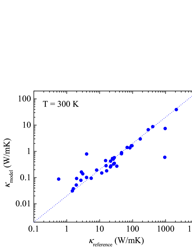
Figure 1: Comparison of intrinsic lattice thermal conductivity calculated from our proposed model with $B_{1}=2/\sqrt{3}$ and the reference value at 300 K, the dotted blue line is $y=x/50$.

However, it was found that there was a quantitative difference in the absolute values between $\kappa_{\text{reference}}$ and our model. The reasons for such a difference might be explained as the following: Firstly, Klemens Klemens (1958) claimed that the quantitative accuracy of the approximation shown as Eq. 5 might not be very reliable. Secondly, the approximations might introduce a factor to the expression of $\kappa_{l}$, which might also be the reason why Julian Julian (1965) needed to fit the factor $B_{2}$ with a digital computer. As such, it is justified to improve our model by fitting the parameter $B_{1}$. Reducing the constant $B_{1}$ by a factor of $1/\sqrt{50}$ will make the calculated intrinsic lattice thermal conductivity increase to 50 times its original value. Therefore, we suggest to use $B_{1}=2/\sqrt{150}$ in the future and we used this value in our following discussions. It should be noted that multiplying a constant number to the calculated thermal conductivity from our model will not change the Pearson and Spearman correlation coefficients. Even without this adjusted value for $B_{1}$, the result calculated from our model can be used as a very good descriptor for intrinsic lattice thermal conductivity.

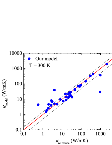
(a)

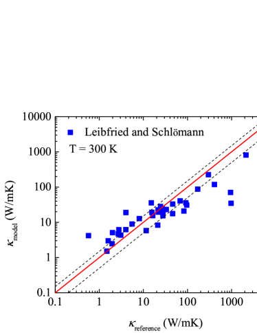
(b)

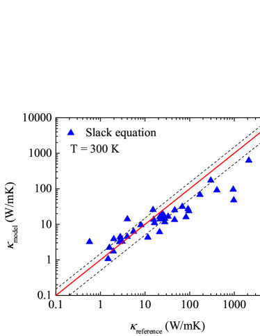
(c)

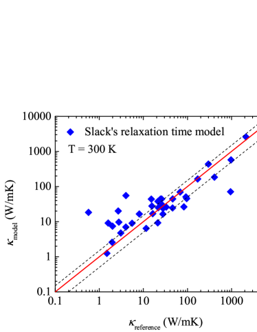
(d)

Figure 2: Intrinsic lattice thermal conductivity at 300 K calculated from (a) our proposed model with $B_{1}=2/\sqrt{150}$, (b) Leibfried and Schlömann’s model, (c) the Slack equation, and (d) Slack’s relaxation time model. The solid red line is $y=x$ and dashed black lines represent $\pm$50% error.

Table 1: Pearson correlation coefficient $r$, Spearman correlation coefficient $\rho$, and average factor difference (AFD) between the thermal conductivity calculated from different models and the reference value at 300 K.

	Our model	Leibfried and Schlömann	Slack equation	Slack’s relaxation time model
$r$	0.898	0.865	0.896	0.906
$\rho$	0.919	0.897	0.908	0.815
AFD	1.649	2.091	2.208	2.174

Figure 2 shows the comparison of intrinsic lattice thermal conductivity from different models at 300 K. We compare our model with Leibfried and Schlömann’s model, the Slack equation, and Slack’s relaxation time models because they are currently widely used. The solid red lines is $y=x$ and is plotted to guide the eye. The dashed black lines indicate $\pm$50% error. The data calculated from these models have been carefully checked and the details can be found in the supplementary materials. We have fully reproduced the result for silicon calculated by Bjerg et al. Bjerg et al. (2014) using the Slack equation. Then we moved forward to use our formulas for $\gamma$ and $\theta_{D}$, and further used different models. The raw data for these figures can also be found in the supplementary materials. From these figures, it can be seen that all these models can predict the qualitative trend of $\kappa_{l}$ reasonably well. As shown in Table 1, we checked the Pearson and Spearman correlation coefficients for different models and found that they are consistently larger than 0.86 and 0.81, respectively. This also indicates that all of these models can give the qualitative trend. By comparing the four models we found that our proposed model showed the largest Spearman correlation coefficient and the second largest Pearson correlation coefficient. We emphasize again here that the Pearson correlation coefficient and Spearman coefficient are not related to the fitting parameter. Pearson correlation coefficient is a measure of the linear relationship Nath et al. (2016) but it is sensitive to the data distribution Wikipedia contributors (2018). For example, the large data points can affect its value significantly. Therefore, in order to give an equal weight to all data points, we further used AFD to quantify the result. With our fitted $B_{1}=2/\sqrt{150}$, our model shows AFD=1.649, which is quite close to unity. By comparison we can find that AFD is closer to unity for our model than that for the other models. From Fig. 2(a) it can be also seen that most of our data points are within the $\pm$50% error lines. It can be thus concluded that our proposed model has the best performance from the comparison.

The reason why our model has the best performance is that we have used less approximations than Leibfried and Schlömann’s model or the Slack equation, and the full phonon dispersion curve is also taken into account. The only part where we have used approximations is in calculating the relaxation time, to be more specific, in three-phonon scattering strength. Besides the better performance, some other advantages of our proposed model are: (i) iterative method can be used with our model, which would be important when Normal processes plays a role, (ii) some important phonon information can be obtained from our model, e.g. the phonon relaxation times. At low temperatures, Normal processes will play a more important role. To show the importance of Normal processes, we also showed the result at 100 K in Fig. 3. Note that we still kept the same $B_{1}$ as the 300 K case.

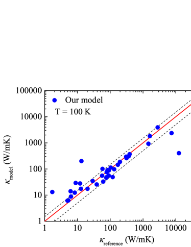
(a)

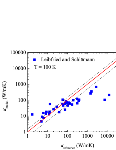
(b)

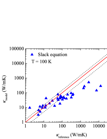
(c)

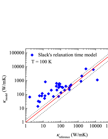
(d)

Figure 3: Intrinsic lattice thermal conductivity at 100 K calculated from (a) our proposed model with $B_{1}=2/\sqrt{150}$, (b) Leibfried and Schlömann’s model, (c) the Slack equation, and (d) Slack’s relaxation time model. The solid red line is $y=x$ and dashed black lines represent $\pm$50% error.

Table 2: Pearson correlation coefficient $r$, Spearman correlation coefficient $\rho$, and average factor difference (AFD) between the thermal conductivity calculated from different models and the reference value at 100 K.

	Our model	Leibfried and Schlömann	Slack equation	Slack’s relaxation time model
$r$	0.977	0.954	0.965	0.980
$\rho$	0.930	0.900	0.912	0.787
AFD	1.730	2.686	2.953	3.841

It can be seen from Fig. 3 that our model has the best performance. Especially, when compared with Leibfried and Schlömann’s model and the Slack equation, our model has better quantitative accuracy for high-thermal-conductivity materials. In Table 2, we also show the correlation coefficients for different models at 100 K. It can be seen that our model shows the largest Pearson and Spearman correlation coefficients and the smallest AFD. The Pearson correlation coefficient is very close to unity because it is sensitive to the largest value in our data. However, the other two correlation coefficient, especially AFD, do not have such an issue and can be used as a good representation of all data points. At 100 K, AFD is 1.730 for our model, which is comparable with the result at 300 K. Nevertheless, the other three models show much worse AFD at 100 K than that at 300 K. This can corroborate the importance of Normal processes and the good performance of our model at low temperatures.

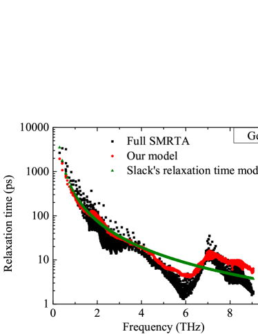
(a) Ge at 300 K

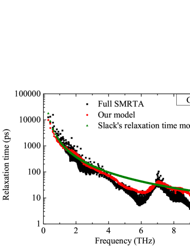
(b) Ge at 100 K

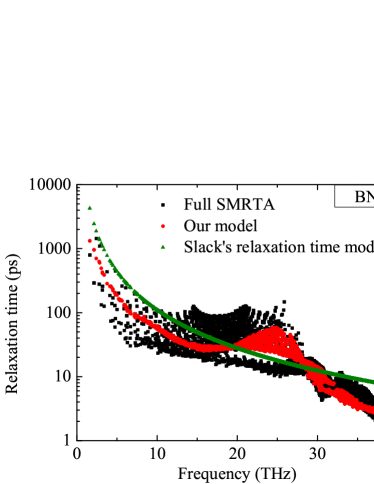
(c) BN at 300 K

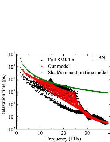
(d) BN at 100 K

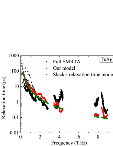
(e) TeAgLi at 300 K

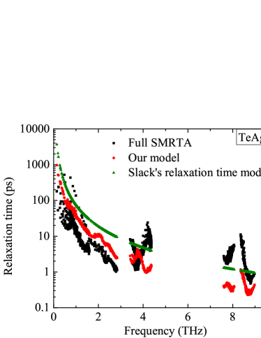
(f) TeAgLi at 100 K

Figure 4: Comparison of the relaxation times calculated from full SMRTA method, our model, and Slack’s relaxation time model.

As we discussed before, another advantage of our model is that some important phonon information can be obtained. In Fig. 4, we further compared the relaxation times calculated from full SMRTA method, our model, and Slack’s relaxation time model. The results for three materials were shown in Fig. 4, where the materials with the highest thermal conductivity value (BN), the typical semiconductor material Ge, and a half-Heusler compound TeAgLi were chosen. The results for the other materials can be found in the supplementary materials. The relaxation times from SMRTA method instead of the iterative method is used in this figure because relaxation times is not well defined in the latter one. It can be found that our model can predict the trend of relaxation times reasonably well, better than Slack’s relaxation time model. Slack’s relaxation time model can only give a rough trend of the relaxation times. It should be noted that the $\omega^{-2}$ trend of relaxation times in Slack’s model may also be questionable Esfarjani et al. (2011). Our model would be physically better in extracting relaxation times compared with Slack’s model as the scattering phase space Lindsay and Broido (2008) information is included in our model. It should be noted that Lindsay has shown the strong relationship of phase space and lattice thermal conductivity Lindsay (2016). The relaxation times computed from Slack’s model deviates even more from the full SMRTA calculation at 100 K than the result at 300 K. Our model shows a good agreement with the full SMRTA calculation at both 100 K and 300 K. Therefore, our model can better characterize the temperature dependence of phonon relaxation times and the lattice thermal conductivity.

V Summary

In summary, we reviewed the approximations used in deriving the Slack equation and identified the necessary approximations at the present time. We proposed a model to calculate lattice thermal conductivity based on the approximation for three-phonon scattering strength, which can be derived from QHA. This model is computationally more efficient than the full calculation and has comparable computational cost but better accuracy than existing QHA methods. The full phonon dispersion curve is taken into account in our model. The results for 37 materials from our proposed model show a strong correlation with the calculated thermal conductivities from full iterative method. We compared our proposed model with other widely-used models, including Leibfried and Schlömann’s model, the Slack equation, and Slack’s relaxation time model, and found that our model has better performance. Our model can take Normal processes into account and has much better performance at low temperatures compared with the other models. Another advantage of our model is that some important phonon information can be obtained, which will enable us to have better understanding about the physics compared with the other high-throughput methods like Slack’s relaxation time model. The better understanding may shed some light on finding high-thermal-conductivity or low-thermal-conductivity materials. Our proposed model finds a balance between accuracy and efficiency and can be very useful because of its quantitative predictive power and low computational cost compared with the full calculation.

Data Availability

The raw data that support the findings of this study are available in the supporting information. The code and scripts for the method proposed in this study are available from the corresponding author upon reasonable request.

Author Contributions

H.X. carried out calculations with comments and ideas from X.G. and H.B. All authors analyzed the data. H.B. supervised the research. H.X. prepared the draft manuscript. X.G. and H.B. commented on, discussed and edited the manuscript.

Competing Interests

The authors declare no competing financial or non-financial interests.

References

- Cahill et al. (2002) D. G. Cahill, W. K. Ford, K. E. Goodson, G. D. Mahan, A. Majumdar, H. J. Maris, R. Merlin, and S. R. Phillpot, Journal of Applied Physics 93, 793 (2002).
- Cahill et al. (2014) D. G. Cahill, P. V. Braun, G. Chen, D. R. Clarke, S. Fan, K. E. Goodson, P. Keblinski, W. P. King, G. D. Mahan, A. Majumdar, H. J. Maris, S. R. Phillpot, E. Pop, and L. Shi, Applied Physics Reviews 1, 011305 (2014).
- Garimella et al. (2012) S. V. Garimella, L. T. Yeh, and T. Persoons, IEEE Transactions on Components, Packaging and Manufacturing Technology 2, 1307 (2012).
- Lindsay et al. (2013a) L. Lindsay, D. A. Broido, and T. L. Reinecke, Physical Review Letters 111, 025901 (2013a).
- Qiu et al. (2012) B. Qiu, H. Bao, G. Zhang, Y. Wu, and X. Ruan, Computational Materials Science 53, 278 (2012).
- Yang et al. (2014) K. Yang, S. Cahangirov, A. Cantarero, A. Rubio, and R. D’Agosta, Physical Review B 89, 125403 (2014).
- Gorai et al. (2016) P. Gorai, D. Gao, B. Ortiz, S. Miller, S. A. Barnett, T. Mason, Q. Lv, V. Stevanović, and E. S. Toberer, Computational Materials Science 112, Part A, 368 (2016).
- van Roekeghem et al. (2016) A. van Roekeghem, J. Carrete, C. Oses, S. Curtarolo, and N. Mingo, Physical Review X 6, 041061 (2016).
- Nath et al. (2017) P. Nath, J. J. Plata, D. Usanmaz, C. Toher, M. Fornari, M. Buongiorno Nardelli, and S. Curtarolo, Scripta Materialia 129, 88 (2017).
- White Paper (2011) M. G. I. White Paper, “Materials Genome Initiative for Global Competitiveness,” https://www.mgi.gov/sites/default/files/documents/materials_genome_initiative-final.pdf (2011), [Online; accessed June 25, 2018].
- Plata et al. (2017) J. J. Plata, P. Nath, D. Usanmaz, J. Carrete, C. Toher, M. Jong, M. Asta, M. Fornari, M. B. Nardelli, and S. Curtarolo, npj Computational Materials 3, 45 (2017).
- Lindsay (2016) L. Lindsay, Nanoscale and Microscale Thermophysical Engineering 20, 67 (2016).
- Li et al. (2014) W. Li, J. Carrete, N. A. Katcho, and N. Mingo, Computer Physics Communications 185, 1747 (2014).
- Togo et al. (2015) A. Togo, L. Chaput, and I. Tanaka, Physical Review B 91, 094306 (2015).
- Carrete et al. (2017) J. Carrete, B. Vermeersch, A. Katre, A. van Roekeghem, T. Wang, G. K. H. Madsen, and N. Mingo, Computer Physics Communications 220, 351 (2017).
- Blanco et al. (2004) M. A. Blanco, E. Francisco, and V. Luaña, Computer Physics Communications 158, 57 (2004).
- Miller et al. (2017) S. A. Miller, P. Gorai, B. R. Ortiz, A. Goyal, D. Gao, S. A. Barnett, T. O. Mason, G. J. Snyder, Q. Lv, V. Stevanović, and E. S. Toberer, Chemistry of Materials 29, 2494 (2017).
- Toher et al. (2014) C. Toher, J. J. Plata, O. Levy, M. de Jong, M. Asta, M. B. Nardelli, and S. Curtarolo, Physical Review B 90, 174107 (2014).
- Nath et al. (2018) P. Nath, D. Usanmaz, D. Hicks, C. Oses, M. Fornari, M. B. Nardelli, C. Toher, and S. Curtarolo, arXiv:1807.04669 [cond-mat.mtrl-sci] (2018).
- Bjerg et al. (2014) L. Bjerg, B. B. Iversen, and G. K. H. Madsen, Physical Review B 89, 024304 (2014).
- Lindsay and Broido (2008) L. Lindsay and D. A. Broido, Journal of Physics: Condensed Matter 20, 165209 (2008).