Sequential Variational Autoencoders for Collaborative Filtering

Abstract.

Variational autoencoders were proven successful in domains such as computer vision and speech processing. Their adoption for modeling user preferences is still unexplored, although recently it is starting to gain attention in the current literature. In this work, we propose a model which extends variational autoencoders by exploiting the rich information present in the past preference history. We introduce a recurrent version of the VAE, where instead of passing a subset of the whole history regardless of temporal dependencies, we rather pass the consumption sequence subset through a recurrent neural network. At each time-step of the RNN, the sequence is fed through a series of fully-connected layers, the output of which models the probability distribution of the most likely future preferences. We show that handling temporal information is crucial for improving the accuracy of the VAE: In fact, our model beats the current state-of-the-art by valuable margins because of its ability to capture temporal dependencies among the user-consumption sequence using the recurrent encoder still keeping the fundamentals of variational autoencoders intact.

1. Introduction

The growing diffusion of Web-based services allows an increasingly large number of users to access and consume online content. People access web pages, purchase items in e-commerce sites, watch online content through streaming services, or interact within social networks and media. Understanding the factors that characterize user preferences and shape their future behavior is crucial in order to provide users with a better experience through the recommendation of new content and data that users are likely to appreciate.

Collaborative filtering approaches to recommendation were extensively investigated by the current literature (Aggarwal, 2016). Among these, latent variable models (Hofmann, 2004; Salakhutdinov and Mnih, 2008b; Wang and Blei, 2011; Kabbur et al., 2013) gained substantial attention, due to their capabilities in modeling the hidden causal relationships that ultimately influence user preferences. Recently, however, new approaches based on neural architectures (see (Zhang et al., 2017a) for a comprehensive survey) were proposed, achieving competitive performance with respect to the current state of the art. Also, new paradigms based on the combination of deep learning and probabilistic latent variable modeling (Kingma and Welling, 2014; Rezende et al., 2014) were proven quite successful in domains such as computer vision and speech processing. However, their adoption for modeling user preferences is still unexplored, although recently it is starting to gain attention (Liang et al., 2018; Li and She, 2017).

The aforementioned approaches rely on the “bag-of-word” assumption: when considering a user and her preferences, the order of such preferences can be neglected and all preferences are exchangeable. This assumption works with general user trends which reflect a long-term behavior. However, it fails to capture the short-term preferences that are specific of several application scenarios, especially in the context of the Web. Sequential data can express causalities and dependencies that require ad-hoc modeling and algorithms. And in fact, efforts to capture this notion of causality have been made, both in the context of latent variable modeling (Rendle et al., 2010; Barbieri et al., 2013; Tavakol and Brefeld, 2014; He et al., 2017a) and deep learning (Hidasi et al., 2016; Devooght and Bersini, 2017; Wu et al., 2017; Tang and Wang, 2018).

In this paper, we consider the task of sequence recommendation from the perspective of combining deep learning and latent variable modeling. Inspired by the approach in (Liang et al., 2018), we assume that at a given timestamp the choice of a given item is influenced by a latent factor that models user trends and preferences. However, the latent factor itself can be influenced by user history and modeled to capture both long-term preferences and short-term behavior. As a matter of fact, the recent studies in the recurrent neural network literature (Chung et al., 2014; Greff et al., 2017; Vaswani et al., 2017) demonstrate the capabilities of these architectures in capturing both long-term and short-term relationships. It is hence natural to exploit them in a variational setting.

Our contribution can be summarized as follows.

• We review the framework of Variational Autoencoders and discuss its adoption for the problem of modeling implicit preferences in a collaborative filtering scenario.

• We extend the framework to the case of sequential recommendation, where user’s preferences exhibit temporal dependencies. In particular, we discuss different modeling alternatives for tackling this task through the adoption of recurrent neural network architectures that model latent dependencies at different abstraction levels.

• We evaluate the proposed framework on standard benchmark datasets, by showing that (a) approaches not considering temporal dynamics are not totally adequate to model user preferences, and (b) the combination of latent variable and temporal dependency modeling produces a substantial gain, even with regard to other approaches that only focus on temporal dependencies through recurrent relationships.

The rest of the paper is organized as follows. Section 2 discusses the recent contributions in the current literature and provides a systematic review of the approaches related to our task of interest. Sections 3 and 4 propose the modeling of user preferences in a variational setting, by illustrating how the general framework can be adapted to the case of temporally ordered dependencies. The effectiveness of the proposed modeling is illustrated in section 5, and pointers to future developments are discussed in section 6.

2. Related Work

Recommender systems have been extensively studied over the last two decades. Within the collaborative filtering framework, recommendation is essentially modeled as a prediction problem: Given a user and an item, we would like to predict the preference of the user for that item, exploiting the user’s past choices, i.e. her history.

Most approaches disregard the temporal order of the preferences in a user’s history. Among these, latent variable models (Hofmann, 2004; Salakhutdinov and Mnih, 2008b, a; Rendle et al., 2009; Agarwal and Chen, 2010; Ning and Karypis, 2011; Wang and Blei, 2011; Rendle, 2012; Kabbur et al., 2013; Barbieri et al., 2014; Barbieri and Manco, 2011) were proven extremely effective in modeling user preferences and providing reliable recommendations. Essentially, these approaches embed users and items into latent spaces that translate relatedness into geometrical closeness. The latent embeddings can be used to decompose the large sparse preference matrix (Salakhutdinov and Mnih, 2008a, b; Agarwal and Chen, 2010), to devise item similarity (Ning and Karypis, 2011; Kabbur et al., 2013), or more generally to parameterize probability distributions for item preference (Rendle et al., 2009; Hofmann, 2004; Wang and Blei, 2011; Rendle, 2012) and sharpen the prediction quality by means of meaningful priors.

The recent literature is currently focusing on deep learning, which shows substantial advantages over traditional approaches. For example, Neural Collaborative Filtering (NCF) (He et al., 2017b) generalizes matrix factorization to a non-linear setting, where users, items and preferences are modeled through a simple multilayer perceptron network that exploits latent factor transformations.

Notably, prominent deep learning approaches to collaborative filtering are based on the idea of autoencoding the features from the preference matrix. AutoRec (Sedhain et al., 2015) exploits autoencoders to encode preference histories. Unseen preferences can be devised by looking at the reconstructed decoding, which is shaped to include scores for all possible items of interest. Autoencoders are also amenable to consider side information (Strub and Mary, 2015) to mitigate the sparsity of the data and to tackle the cold start problem.

Hybrid approaches that integrate latent variable modeling and deep learning have also gained attention. Collaborative Deep Learning (Wang et al., 2015) embeds a stacked denoising autoencoder (Vincent et al., 2010) into a Bayesian matrix factorization setting. Similarly, AutoSVD++ (Zhang et al., 2017b) exploits the notion of contractive autoencoder (Rifai et al., 2011) to learn latent item representations that are integrated into the SVD++ model (Koren, 2008).

The introduction of the variational autoencoding framework (Kingma and Welling, 2014; Rezende et al., 2014) has suggested a tighter coupling between deep learning and latent variable modeling. Collaborative Variational Autoencoder (CVA) (Li and She, 2017) and Hybrid Variational Autoencoder (HVAE) (Gupta et al., 2018) exploit side information to feed a variational autoencoder whose goal is to produce a latent representation of the items. In CVA, the preference matrix is hence modeled by combining user and item embeddings with the item latent representations, while HVAE uses another variational autoencoder to reproduce the whole users’ preference history. By contrast, (Liang et al., 2018) proposes a neural generative model where a user’s history is modeled through a multinomial likelihood conditioned to a latent user representation which in turn is modeled through a variational autoencoder.

Within the context of collaborative filtering, a strong effort has also been made to model temporal dynamics within the history of user preferences (Quadrana et al., 2018). The Factorizing Personalized Markov Chain model (FPMC) (Rendle et al., 2010), for example, proposes a combination of matrix factorization and Markov chains. FPMC considers personalized first-order transition probabilities between items, which are modeled by decomposing the underlying tensor through user and item embeddings. Transition probabilities can also be measured by exploiting more sophisticated modeling (He and McAuley, 2016; He et al., 2017a), where users are mapped into translation (latent) vectors operating on item sequences and consequently a transition corresponds to a geometric affinity of these latent vectors. Orthogonally, Markov dependencies can also be exploited to model dependencies between latent variables (Barbieri et al., 2013), thus resulting in richer formalizations and more accurate recommendations.

Recently, a revamped interest for sequence-based recommendation has taken place, motivated by both the success of recurrent neural networks (Cho et al., 2014; Greff et al., 2017) in domains such as language modeling, and the need to focus on session-based recommendations (Hidasi et al., 2016; Tan et al., 2016), i.e. recommendation that do not rely on a user model and instead can cope with single anonymous preference sessions.

GRU4Rec (Hidasi et al., 2016) proposes a recurrent neural network model based on Gated Recurrent Units to predict the next item in a user session, based on the history seen so far. Since its introduction, this model has witnessed several evolutions, and similar architectures were proposed in (Devooght and Bersini, 2017; Liu et al., 2016; Twardowski, 2016; Wu et al., 2016; Tan et al., 2016; Jannach and Ludewig, 2017; Quadrana et al., 2017). Recurrent networks were also exploited to strengthen matrix factorization, by producing history-aware embeddings of users and items. The RRN approach proposed in (Wu et al., 2017) combines two recurrent networks, whose output at any time-step, relative to a specific user and item, can be hence exploited to predict the current preference.

Finally, the CASER (Convolutional Sequence Embedding Recommendation) model (Tang and Wang, 2018) proposes an approach that departs from RNN modeling and instead exploits a convolutional neural network, by transforming a sequence into a matrix built from the concatenation of the embeddings of the items appearing in the sequence. The matrix can hence feed convolutional layers that can extract relevant useful features for predicting the next items.

3. Background

The framework of variational autoencoders draws from the idea of latent variable modeling (Murphy, 2012). Essentially, we can assume a $K$-dimensional latent variable space $\mathcal{Z}$, upon which we can devise a probability density function $P_{\theta}(\bm{\mathit{z}})$ for $\bm{\mathit{z}}\in\mathcal{Z}$, where $\theta$ represents a set of density parameters. The datapoints $\bm{\mathit{X}}=\left\{\bm{\mathit{x}}_{1},\ldots,\bm{\mathit{x}}_{M}\right\}$ we observe can be modeled through a dependency $P_{\phi}(\bm{\mathit{x}}|\bm{\mathit{z}})$, so that the overall likelihood of $\bm{\mathit{X}}$ can be specified by marginalizing over $\mathcal{Z}$:

$$P(\bm{\mathit{X}})= \prod_{i}P(\bm{\mathit{x}}_{i})=\prod_{i}\int P_{\phi}\left(\bm{\mathit{x}}_{i}|\bm{\mathit{z}}\right)P_{\theta}(\bm{\mathit{z}})\mathop{\mathrm{\mathstrut d}}\nolimits\!\bm{\mathit{z}}\,.$$

Within the classical VAE framework (Kingma and Welling, 2014; Rezende et al., 2014), $\bm{\mathit{z}}$ is assumed to be distributed according to a standard normal distribution, that is $\theta=\{\mathbf{0},\mathbf{I}_{K}\}$ and consequently $\mathbf{z}\sim\mathcal{N}(\mathbf{0},\mathbf{I}_{K})$. The key intuition here is that even complex dependencies can be generated starting from normally distributed variables. Thus, $P_{\phi}(\bm{\mathit{x}}_{i}|\bm{\mathit{z}})$ is parameterized by the function $f_{\phi}(\bm{\mathit{z}})$, representing any (unknown) transformation of $z$ that expresses such a dependency. We can model this transformation through a neural network, so that $\phi$ represents the set of network parameters to be optimized. Hence, we can model the inference problem for $P(\bm{\mathit{X}})$ as optimization problem, where we aim at finding the optimal parameter set $\phi$ that maximize $P(\bm{\mathit{X}})$.

However, $P(\bm{\mathit{X}})$ is typically intractable and we need to find an approximation. Variational inference (Blei et al., 2017) usually tackles this approximation by introducing a proposal distribution $Q(\bm{\mathit{z}}|\bm{\mathit{x}})$, which approximates the true posterior $P(\bm{\mathit{z}}|\bm{\mathit{x}})$. The relationship between the likelihood and the proposal distribution is given by the following equation:

$$\log P(\mathbf{x}) =\int Q(\bm{\mathit{z}}|\bm{\mathit{x}})\log P(\bm{\mathit{x}})\mathop{\mathrm{\mathstrut d}}\nolimits\!\bm{\mathit{z}}$$

$$=\int Q(\bm{\mathit{z}}|\bm{\mathit{x}})\log\frac{P(\bm{\mathit{x}}|\bm{\mathit{z}})P(\bm{\mathit{z}})}{P(\bm{\mathit{z}}|\bm{\mathit{x}})}\mathop{\mathrm{\mathstrut d}}\nolimits\!\bm{\mathit{z}}$$

$$=\int Q(\bm{\mathit{z}}|\bm{\mathit{x}})\log P(\bm{\mathit{X}}|\bm{\mathit{z}})\mathop{\mathrm{\mathstrut d}}\nolimits\!\bm{\mathit{z}}+\int Q(\bm{\mathit{z}}|\bm{\mathit{x}})\log\frac{Q(\bm{\mathit{z}}|\bm{\mathit{x}})}{P(\bm{\mathit{z}}|\bm{\mathit{x}})}\mathop{\mathrm{\mathstrut d}}\nolimits\!\bm{\mathit{z}}$$

$$-\int Q(\bm{\mathit{z}}|\bm{\mathit{x}})\log\frac{Q(\bm{\mathit{z}}|\bm{\mathit{x}})}{P(\bm{\mathit{z}})}\mathop{\mathrm{\mathstrut d}}\nolimits\!\bm{\mathit{z}}$$

$$=E_{z\sim Q}[\log P(\bm{\mathit{x}}|\bm{\mathit{z}})]+\mathit{KL}\left(Q(\bm{\mathit{z}}|\bm{\mathit{x}})\|P(\bm{\mathit{z}}|\bm{\mathit{x}})\right)$$

$$-\mathit{KL}\left(Q(\bm{\mathit{z}}|\bm{\mathit{x}})\|P(\bm{\mathit{z}})\right)\,.$$

By rearranging, we obtain

(3.1) $$\begin{split}\log P(\mathbf{x})&-\mathit{KL}\left[Q(\bm{\mathit{z}}|\bm{\mathit{x}})\|P(\bm{\mathit{z}}|\bm{\mathit{x}})\right]\\ &=E_{z\sim Q}[\log P(\bm{\mathit{x}}|\bm{\mathit{z}})]-\mathit{KL}\left[Q(\bm{\mathit{z}}|\bm{\mathit{x}})\|P(\bm{\mathit{z}})\right]\,.\end{split}$$

This equation is crucial to the development variational autoencoders. The left-hand side represents the term to maximize, plus an error term due to approximating the true posterior $P(\bm{\mathit{z}}|\bm{\mathit{x}})$ with $Q(\bm{\mathit{z}}|\bm{\mathit{x}})$. A good choice of $Q$ gives a small (hopefully zero) approximation error, and consequently allows to directly optimize the likelihood. The right-hand side of the equation (called Evidence Lower Bound, ELBO) represents the equivalent of the left-hand side, but with the added bonus that, for a given choice of $Q$ it becomes tractable and amenable to optimization. In particular, by noticing that

$$\begin{split}\mathit{KL}&\left[\mathcal{N}(\bm{\mathit{\mu}},\bm{\mathit{\Sigma}})\|\mathcal{N}(\bm{\mathit{m}},\bm{\mathit{S}})\right]=\\ &\frac{1}{2}\left(log\frac{|\bm{\mathit{S}}|}{|\bm{\mathit{\Sigma}}|}-K+\mathit{tr}\left(\bm{\mathit{S}}^{-1}\bm{\mathit{\Sigma}}\right)+\left(\bm{\mathit{m}}-\bm{\mathit{\mu}}\right)^{T}\bm{\mathit{S}}^{-1}\left(\bm{\mathit{m}}-\bm{\mathit{\mu}}\right)\right)\,,\end{split}$$

we can choose to model $Q(\bm{\mathit{z}}|\bm{\mathit{x}})=\mathcal{N}(\bm{\mathit{z}}|\mu_{\lambda}(\bm{\mathit{x}}),\Sigma_{\lambda}(\bm{\mathit{x}}))$, so that the term $\mathit{KL}\left[Q(\bm{\mathit{z}}|\bm{\mathit{x}})\|P(\bm{\mathit{z}})\right]$ has a closed form. Again, we can model the parameters $\mu_{\lambda}(\bm{\mathit{x}})$ and $\Sigma_{\lambda}(\bm{\mathit{x}})$ through a neural network trained on $\bm{\mathit{x}}$ and parameterized by $\lambda$. A particular case that we shall use throughout this paper is given by $\bm{\mathit{\Sigma}}_{\lambda}(\bm{\mathit{x}})=\mathit{diag}\left(\sigma_{\lambda,1}(\bm{\mathit{x}}),\ldots,\sigma_{\lambda,K}(\bm{\mathit{x}})\right)$.

As a consequence, the modeling can resort to two neural networks: the first one for “encoding” an input $\bm{\mathit{x}}$ into a latent variable $\bm{\mathit{z}}$ by means of $Q_{\lambda}(\bm{\mathit{z}}|\bm{\mathit{x}})$. The second one “decodes” the latent representation $\bm{\mathit{z}}$ into the corresponding $\bm{\mathit{x}}$ by means of $P_{\phi}(\bm{\mathit{x}}|\bm{\mathit{z}})$. The learning process is governed by the loss function given by the right-hand side of eq. 3.1, computed on the training data $\bm{\mathit{X}}$.

A problem with this loss is that term $E_{\bm{\mathit{z}}\sim Q}[\log P(\bm{\mathit{x}}|\bm{\mathit{z}})]$ is typically approximated by sampling the values $\bm{\mathit{z}}$ according to $Q(\bm{\mathit{z}}|\bm{\mathit{x}})$. However, the sampling is a nondeterministic function that depends on the parameters $\bm{\mathit{\mu}}_{\lambda}$ and $\bm{\mathit{\Sigma}}_{\lambda}$ (which in turn depend on $\lambda$) and is not differentiable. To overcome this, (Kingma and Welling, 2014) propose a reparametrization trick: instead of sampling $\bm{\mathit{z}}$, we can sample an auxiliary noise variable $\bm{\mathit{\epsilon}}$ according to a fixed distribution $P(\bm{\mathit{\epsilon}})$, and obtain $\bm{\mathit{z}}$ by means of a differentiable transformation depending on $\lambda,\bm{\mathit{\epsilon}}$ and $\bm{\mathit{x}}$. Specifically, we can sample gaussian noise $\bm{\mathit{\epsilon}}\sim\mathcal{N}(\bm{\mathit{0}},\bm{\mathit{I}})$, and obtain $\bm{\mathit{z}}_{\lambda}(\bm{\mathit{\epsilon}},\bm{\mathit{x}}_{i})=\bm{\mathit{\mu}}_{\lambda}(\bm{\mathit{x}}_{i})+\bm{\mathit{\Sigma}}_{\lambda}(\bm{\mathit{x}}_{i})\cdot\bm{\mathit{\epsilon}}$, normally distributed according to parameters $\bm{\mathit{\mu}}_{\lambda}$ and $\bm{\mathit{\Sigma}}_{\lambda}$.

To summarize, given the loss function

(3.2) $$\begin{split}\mathcal{L}(\phi,\lambda;\bm{\mathit{X}})=\sum_{i}&\left\{\frac{1}{2}\sum_{k}\left(\sigma_{\lambda,k}(\bm{\mathit{x}}_{i})-1-\log\sigma_{\lambda,k}(\bm{\mathit{x}}_{i})+\mu_{\lambda,k}(\bm{\mathit{x}}_{i})^{2}\right)\right.\\ &-\left.\vphantom{\sum_{k}k}E_{\bm{\mathit{\epsilon}}\sim\mathcal{N}(\bm{\mathit{0}},\bm{\mathit{I}})}\left[\log P_{\phi}\left(\bm{\mathit{x}}_{i}|\bm{\mathit{z}}_{\lambda}(\bm{\mathit{\epsilon}},\bm{\mathit{x}}_{i})\right)\right]\right\}\,,\end{split}$$

we can learn the parameters $\lambda$ and $\phi$, and consequently the encoder $Q_{\lambda}(\bm{\mathit{z}}|\bm{\mathit{x}})$ and the decoder $P_{\phi}(\bm{\mathit{x}}|\bm{\mathit{z}})$.

4. Variational Autoencoders for User Preferences

The general framework described in the previous section can be instantiated to the case of collaborative filtering by specifying the $\bm{\mathit{x}}$ variables, and consequently the probability density $P_{\phi}(\bm{\mathit{x}}|\bm{\mathit{z}})$. We analyze some alternative models here. We shall use the following shared notation: $u\in U=\{1,\ldots,M\}$ indexes a user and $i\in I=\{1,\ldots,N\}$ indexes an item for which the user can express a preference. We model implicit feedback, thus assuming a preference matrix $\bm{\mathit{X}}\in\{0,1\}^{N\times M}$, so that $\bm{\mathit{x}}_{u}$ represents the (binary) row with all the item preferences for user $u$. Given $\bm{\mathit{x}}_{u}$, we define $I_{u}=\{i\in I|x_{u,i}=1\}$ (with $N_{u}=|I_{u}|$). Analogously, $U_{i}=|\{u\in U|x_{u,i}=1\}|$ and $M_{i}=|U_{i}|$.

We also consider a precedence and temporal relationships within $\bm{\mathit{X}}$. First of all, the preference matrix induces a natural ordering relationship between items: $i\prec_{u}j$ has the meaning that $x_{u,i}>x_{u,j}$ in the rating matrix. Also, we assume the existence of timing information $\bm{\mathit{T}}\in{\rm I\!R}_{+}^{M\times N}\cup\{\emptyset\}$, where the term $t_{u,i}$ represents the time when $i$ was chosen by $u$ (with $t_{u,i}=\emptyset$ if $x_{u,i}=0$). Then, $i<_{u}j$ denotes that $t_{u,i}<t_{u,j}$, With an abuse of notation, we also introduce a temporal mark in the elements of $\bm{\mathit{x}}_{u}$: the term $\bm{\mathit{x}}_{u(t)}$ (with $1\leq t\leq N_{u}$) represents the $t$-th item in $I_{u}$ in the sorting induced by $<_{u}$, whereas $\bm{\mathit{x}}_{u(1:t)}$ represents the sequence $\bm{\mathit{x}}_{u(1)},\ldots,\bm{\mathit{x}}_{u(t)}$.

4.1. Multinomial model

The reference model is the Multinomial variational autoencoder (MVAE) proposed in (Liang et al., 2018). Within this framework, for a given user $u$ it is possible to devise $\bm{\mathit{x}}_{u}$ according to the generative setting:

(4.1) $$\begin{gathered}\bm{\mathit{z}}_{u}\sim\mathcal{N}(\bm{\mathit{0}},\bm{\mathit{I}}_{K})\,,\qquad\pi(\bm{\mathit{z}}_{u})\sim\exp\left\{f_{\phi}(\bm{\mathit{z}}_{u})\right\}\,,\\ \bm{\mathit{x}}_{u}\sim\mathit{Multi}\left(N_{u},\pi(\bm{\mathit{z}}_{u})\right)\,.\end{gathered}$$

The underlying “decoder” is modeled by

$$\log P_{\phi}(\bm{\mathit{x}}_{u}|\bm{\mathit{z}}_{u})=\sum_{i}x_{u,i}\log\pi_{i}(\bm{\mathit{z}}_{u})\,,$$

thus enabling a complete specification of the overall variational framework. Prediction for new items is accomplished by resorting to the learned functions $f_{\phi}$ and $Q_{\lambda}$: given a user history $\bm{\mathit{x}}$, we compute $\bm{\mathit{z}}=\bm{\mathit{\mu}}_{\lambda}(\bm{\mathit{x}})$ and then devise the probabilities for the whole item set through $\pi(\bm{\mathit{z}})$. Unseen items can then be ranked according to their associated probabilities.

4.2. Ranking Models

A different formulation is inspired by the Bayesian Personalized Ranking (BPR) model introduced in (Rendle et al., 2009). Here, we explicitly model an order among observations, so that for each triplet $u,i,j$ we can devise whether $i\prec_{u}j$. In classical BPR, this is modeled by associating a factorization rank $\bm{\mathit{p}}^{T}_{u}\bm{\mathit{q}}_{i}$ for each pair $(u,i)$, and requiring that $\bm{\mathit{p}}^{T}_{u}\bm{\mathit{q}}_{i}<\bm{\mathit{p}}^{T}_{u}\bm{\mathit{q}}_{j}$ whenever $i\prec_{u}j$. In a VAE setting, $\bm{\mathit{p}}^{T}_{u}\bm{\mathit{q}}_{i}$ is replaced by a score based on the latent gaussian variable $\bm{\mathit{z}}_{u,i}$:

(4.2) $$\begin{gathered}\bm{\mathit{z}}_{u,i}\sim\mathcal{N}(\bm{\mathit{0}},\bm{\mathit{I}}_{K})\,,\\ i\prec_{u}j\sim\mathit{Bernoulli}\left(\pi(\bm{\mathit{z}}_{u,i},\bm{\mathit{z}}_{u,j})\right)\,,\end{gathered}$$

Two different specifications for $\pi(\bm{\mathit{z}}_{u,i},\bm{\mathit{z}}_{u,j})$ are possible: either we let the neural network implicitly models the comparison between $i$ and $j$

(4.3) $$\pi(\bm{\mathit{z}}_{u,i},\bm{\mathit{z}}_{u,j})\sim\sigma\left(f_{\phi}(\bm{\mathit{z}}_{u,i},\bm{\mathit{z}}_{u,j})\right)\,,$$

or alternatively, we can assume that the network simply provides the score upon which to compare:

(4.4) $$\pi(\bm{\mathit{z}}_{u,i},\bm{\mathit{z}}_{u,j})\sim\sigma\left(f_{\phi}(\bm{\mathit{z}}_{u,j})-f_{\phi}(\bm{\mathit{z}}_{u,i})\right)\,.$$

Here, $\sigma$ represents the standard logistic function $\sigma(z)=1/(1+\exp\{-z\})$.

These alternatives represent two different instantiations of the Ranking Variational Autoencoder. The difference between them is substantial at prediction time: given $u$ and a set $J\subset I$ of unseen items, in both models we need to devise $\bm{\mathit{z}}_{u,i}=\bm{\mathit{\mu}}_{\lambda}(\bm{\mathit{x}}_{u}|x_{u,i}=1)$ for each $i\in J$. However, the instance of eq. 4.3 requires to organize the data as triplets $u,i,j$ and to compute $P_{\phi}(i\prec_{u}j)$ for each triplet. These probabilities can be then exploited to devise an order among the items in $U$. Inconsistencies can arise in this setting, which can in principle prevent to produce a global rank order.

Conversely, the instance of eq. 4.4 can directly sort items according to $f_{\phi}(\bm{\mathit{z}}_{u,i})$ and does not produce inconsistencies, thus being better suited for ranking items. In the following we shall only focus on this instance, that we shall refer to as RVAE.

4.3. Sequential Models

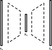
(a) MVAE

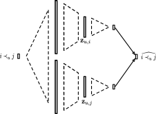
(b) RVAE

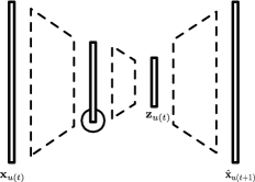
(c) SVAE

Figure 1. Variational architectures. Terms with hat represent decoding reconstruction. Dotted boxes represent neural layers.

The basic framework proposed in section 3 can also be exploited to model time-aware user preferences. Ideally, latent variable modeling should be able to express temporal dynamics and hence causalities and dependencies among preferences in a user’s history. In the following we elaborate on this intuition.

4.3.1. Modeling History-aware User Preferences

Within a probabilistic framework, we can model temporal dependencies by conditioning each event to the previous events: given a sequence $\bm{\mathit{x}}_{(1:T)}$, we have

$$P\left(\bm{\mathit{x}}_{(1:T)}\right)=\prod_{t=0}^{T-1}P\left(\bm{\mathit{x}}_{(t+1)}|\bm{\mathit{x}}_{(1:t)}\right)\,.$$

This specification suggests two key aspects:

• There is a recurrent relationship between $\bm{\mathit{x}}_{(t+1)}$ and $\bm{\mathit{x}}_{(1:t)}$ devised by $P\left(\bm{\mathit{x}}_{(t+1)}|\bm{\mathit{x}}_{(1:t)}\right)$, upon which the modeling can take advantage, and

• each time-step can be handled separately, and in particular it can be modeled through a conditional VAE.

Let us consider the following (simple) generative model

(4.5) $$\begin{gathered}\bm{\mathit{z}}_{u(t)}\sim\mathcal{N}\left(\bm{\mathit{0}},\bm{\mathit{I}}_{K}\right)\,,\qquad\pi\left(\bm{\mathit{z}}_{u(t)}\right)\sim\exp\left\{f_{\phi}\left(\bm{\mathit{z}}_{u(t)}\right)\right\}\,,\\[5.69054pt] \bm{\mathit{x}}_{u(t)}\sim\mathit{Multi}\left(1,\pi\left(\bm{\mathit{z}}_{u(t)}\right)\right)\,,\end{gathered}$$

which results in the joint likelihood

$$P(\bm{\mathit{x}}_{u(1:T)},\bm{\mathit{z}}_{u(1:T)})=\prod_{t}P(\bm{\mathit{x}}_{u(t)}|\bm{\mathit{z}}_{u(t)})P(\bm{\mathit{z}}_{u(t)})\,.$$

Here, we can approximate the posterior $P(\bm{\mathit{z}}_{u(1:T)}|\bm{\mathit{x}}_{u(1:T)})$ with the factorized proposal distribution

$$Q_{\lambda}(\bm{\mathit{z}}_{u(1:T)}|\bm{\mathit{x}}_{(1:T)})=\prod_{t}q_{\lambda}(\bm{\mathit{z}}_{u(t)}|\bm{\mathit{x}}_{(1:t-1)})\,,$$

where $q_{\lambda}(\bm{\mathit{z}}_{u(t)}|\bm{\mathit{x}}_{(1:t-1)})$ is a gaussian distribution whose parameters $\bm{\mathit{\mu}}_{\lambda}(t)$ and $\bm{\mathit{\sigma}}_{\lambda}(t)$ depend upon the current history $\bm{\mathit{x}}_{u(1:t-1)}$, by means of a recurrent layer $\bm{\mathit{h}}_{t}$:

(4.6) $$\begin{split}\bm{\mathit{\mu}}_{\lambda}(t),\bm{\mathit{\sigma}}_{\lambda}(t)&=\varphi_{\lambda}(\bm{\mathit{h}}_{t})\\ \bm{\mathit{h}}_{t}&=\mathit{RNN}_{\lambda}\left(\bm{\mathit{h}}_{t-1},\bm{\mathit{x}}_{u(t-1)}\right)\,.\end{split}$$

The resulting loss function follows directly from eq. 3.2:

$$\begin{split}\mathcal{L}(\phi,\lambda,\bm{\mathit{X}})=\sum_{u}\sum_{t=1}^{N_{u}}&\left\{\frac{1}{2}\sum_{k}\left(\sigma_{\lambda,k}(t)-1-\log\sigma_{\lambda,k}(t)+\mu_{\lambda,k}(t)^{2}\right)\right.\\ &-\left.\vphantom{\sum_{k}k}E_{\bm{\mathit{\epsilon}}\sim\mathcal{N}(\bm{\mathit{0}},\bm{\mathit{I}})}\left[\log P_{\phi}\left(\bm{\mathit{x}}_{u(t)}|\bm{\mathit{z}}_{\lambda}(\bm{\mathit{\epsilon}},t)\right)\right]\right\}\,.\end{split}$$

The proposal distribution introduces a dependency of the latent variable from a recurrent layer, which allows to recover the information from the previous history. We call this model SVAE. Figure 1 shows the main architectural difference with respect to the models proposed so far. In SVAE, we can observe the recurrent relationship occurring in the layer upon which $\bm{\mathit{z}}_{u(t)}$ depends.

Notably, the prediction step can be easily accomplished in a similar way as for MVAE: given a user history $\bm{\mathit{x}}_{u(1:t-1)}$, we can resort to eq. 4.6 and set $\bm{\mathit{z}}=\bm{\mathit{\mu}}_{\lambda}(t)$, upon which we can devise the probability for the $\bm{\mathit{x}}_{u(t)}$ by means of $\pi(\bm{\mathit{z}})$.

4.3.2. A taxonomy of sequential variational autoencoders

We already discussed that within a sequence modeling framework, the core of the approach is on modeling $P\left(\bm{\mathit{x}}_{(t+1)}|\bm{\mathit{x}}_{(1:t)}\right)$ through a conditional variational autoencoder. SVAE describes just one of several possible modeling choices.

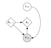
$\scriptscriptstyle P\left(\bm{\mathit{x}}_{(1:T)}\right)=\int P\left(\bm{\mathit{z}}_{(1:T)}\right)\prod_{t=1}^{T-1}P_{\phi}\left(\bm{\mathit{x}}_{(t+1)}|\bm{\mathit{z}}_{(t+1)},\bm{\mathit{x}}_{(1:t)}\right)\mathop{\mathrm{\mathstrut d}}\nolimits\!\bm{\mathit{z}}_{(1:T)}$

(a) Single latent dependency

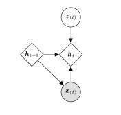
$\scriptscriptstyle P\left(\bm{\mathit{x}}_{(1:T)}\right)=\int P\left(\bm{\mathit{z}}_{(1:T)}\right)\prod_{t=1}^{T-1}P_{\phi}\left(\bm{\mathit{x}}_{(t+1)}|\bm{\mathit{z}}_{(1:t)},\bm{\mathit{x}}_{(1:t)}\right)\mathop{\mathrm{\mathstrut d}}\nolimits\!\bm{\mathit{z}}_{(1:T)}$

(b) Multiple latent dependencies

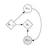
$\scriptscriptstyle P\left(\bm{\mathit{x}}_{(1:T)}\right)=\int\prod_{t=1}^{T-1}P_{\phi}\left(\bm{\mathit{x}}_{(t+1)}|\bm{\mathit{z}}_{(t+1)}\right)P\left(\bm{\mathit{z}}_{(t+1)}|\bm{\mathit{x}}_{(1:t)}\right)\mathop{\mathrm{\mathstrut d}}\nolimits\!\bm{\mathit{z}}_{(1:T)}$

(c) Recurrent latent dependency

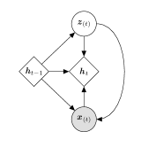
$\scriptscriptstyle P\left(\bm{\mathit{x}}_{(1:T)}\right)=\int\prod_{t=1}^{T-1}P_{\phi}\left(\bm{\mathit{x}}_{(t+1)}|\bm{\mathit{z}}_{(1:t+1)},\bm{\mathit{x}}_{(1:t)}\right)P\left(\bm{\mathit{z}}_{(t+1)}|\bm{\mathit{z}}_{(1:t)},\bm{\mathit{x}}_{(1:t)}\right)\mathop{\mathrm{\mathstrut d}}\nolimits\!\bm{\mathit{z}}_{(1:T)}$

(d) Global recurrent dependency

Figure 2. Recurrent Variational Autoencoders. Diamond boxes represent deterministic variables.

In fact, four alternate formalizations can take place, as illustrated in fig. 2:

• The simplest modeling, considers a single gaussian variable $\bm{\mathit{z}}$ and a parameterization of the conditional distribution $P_{\phi}\left(\bm{\mathit{x}}_{(t+1)}|\bm{\mathit{z}},\bm{\mathit{x}}_{(1:t)}\right)$ with a function $f_{\phi}(\bm{\mathit{z}},\bm{\mathit{h}}_{t+1})$, where $\bm{\mathit{h}}_{t}$ represents the hidden state of a recurrent neural function

  (4.7) $$\bm{\mathit{h}}_{t}=\mathit{RNN}\left(\bm{\mathit{h}}_{t-1},\bm{\mathit{x}}_{(t)}\right)\,.$$

  Figure 2(a) illustrates the graphical model and the sequence likelihood.

• Following (Bayer and Osendorfer, 2014), we can alternatively introduce $t$ independent gaussian variables and parameterize the conditional likelihood $P_{\phi}\left(\bm{\mathit{x}}_{(t+1)}|\bm{\mathit{z}}_{(1:t)},\bm{\mathit{x}}_{(1:t)}\right)$ by means of a function $f_{\phi}(\bm{\mathit{h}}_{t+1})$, where again $\bm{\mathit{h}}_{t}$ represents the hidden state of a recurrent neural function

  (4.8) $$\bm{\mathit{h}}_{t}=\mathit{RNN}\left(\bm{\mathit{h}}_{t-1},\bm{\mathit{x}}_{(t)},\bm{\mathit{z}}_{(t)}\right)\,.$$

  Figure 2(b) illustrates the graphical model and the sequence likelihood.

• So far, the modeling combines history and latent variables to define the conditional distribution. An alternative consists in assuming that history affects the latent variable $\bm{\mathit{z}}$ instead. In practice, the conditional likelihood $P_{\phi}\left(\bm{\mathit{x}}_{(t+1)}|\bm{\mathit{z}}_{(t+1)}\right)$ would only depend on the latent variable, which exhibits a prior distribution $P\left(\bm{\mathit{z}}_{(t+1)}|\bm{\mathit{x}}_{(1:t)}\right)$, modeled as a gaussian with parameters depending on the current state $\bm{\mathit{h}}_{t}$ of the network, devised as in eq. 4.7. The graphical model and sequence likelihood are shown in fig. 2(c) and it resembles the SVAE model discussed above.

• Finally, (Chung et al., 2015) propose a comprehensive model, where the gaussian latent variables $t+1$ also depend on each other through the Markovian dependency $P\left(\bm{\mathit{z}}_{(t+1)}|\bm{\mathit{z}}_{(1:t)},\bm{\mathit{x}}_{(1:t)}\right)$. Both this dependency and $P_{\phi}\left(\bm{\mathit{x}}_{(t+1)}|\bm{\mathit{z}}_{(1:t+1)},\bm{\mathit{x}}_{(1:t)}\right)$ can be specified by the hidden state $\bm{\mathit{h}}_{t}$ of a recurrent network, devised as in eq. 4.8. The graphical model and sequence likelihood are shown in fig. 2(d).

4.3.3. Extending SVAE

The generative model of eq. 4.5 only focuses on the next item in the sequence. The base model however is flexible enough to extend its focus on the next $k$ items, regardless of the time:

$$\bm{\mathit{x}}_{u(t:t+k-1)}\sim\mathit{Multi}\left(k,\pi\left(\bm{\mathit{z}}_{u(t)}\right)\right),$$

Again, the resulting joint likelihood can be modeled in different ways. The simplest way consists in considering $\bm{\mathit{x}}$ as a time-ordered multi-set,

(4.9) $$P(\bm{\mathit{x}}_{u(1:T)},\bm{\mathit{z}}_{u(1:T)})=\prod_{t}P(\bm{\mathit{x}}_{u(t:t+k-1)}|\bm{\mathit{z}}_{u(t)})P(\bm{\mathit{z}}_{u(t)})\,.$$

Alternatively, we can consider the probability of an item as a mixture relative to all the time-steps where it is considered:

(4.10) $$P(\bm{\mathit{x}}_{u(1:T)},\bm{\mathit{z}}_{u(1:T)})=\prod_{t}P(\bm{\mathit{z}}_{u(t)})\sum_{t-k+1\leq j\leq t}P(\bm{\mathit{x}}_{u(t)}|\bm{\mathit{z}}_{u(j)}),$$

where $P(\bm{\mathit{x}}_{u(t)}|\bm{\mathit{z}}_{u(j)})$ is the probability of observing $\bm{\mathit{x}}_{u(t)}$ according to $\pi(\bm{\mathit{z}}_{u(j)})$. In both cases, the variational approximation is modeled exactly as shown above, and the only difference lies in the second component of the loss function, which has to be adapted according to the above equations.

There is an interesting analogy between eq. 4.10 and the attention mechanism (Vaswani et al., 2017). In fact, it can be noticed in the equation that the prediction of $\bm{\mathit{x}}_{u(t)}$ depends on the latent status of the $k$ previous steps in the sequence. In practice, this enables to capture short-term dependencies and to encapsulate them in the same probabilistic framework by weighting the likelihood based on $\bm{\mathit{z}}_{u(t-k+1)},\ldots,\bm{\mathit{z}}_{u(t)}$.

5. Evaluation

We evaluate SVAE on some benchmark datasets, by comparing with various baselines and the current state-of-the-art competitors, in order to assess its capabilities in modeling preference data. Additionally, we provide a sensitivity analysis relative to the configurations/contour conditions upon which SVAE is better suited. The main highlight from our experiments is that SVAE provides a huge edge over the current state-of-the-art for the task of top-N recommendation across various metrics.

5.1. Datasets

We evaluate our model along with the competitors on two popular publicly available datasets, namely Movielens-1M and Netflix. Movielens-1M is a time series dataset containing user-item ratings pairs along with the corresponding timestamp. Since we work on implicit feedback, we binarize the data, by considering only the user-item pairs where the rating provided by the user was strictly greater than 3 on a range 1:5. Netflix has the same data format as Movielens-1M and the same technique is used to binarize the ratings. We use a subset of the full dataset that matches the user-distribution with the full dataset. The subset is built by stratifying users according to their history length, and then sampling a subset of size inversely proportional to the size of the strata. Figure 3 compares the distributions of the full and the sampled dataset: We can notice that the distributions share the same shape, but in the sample users with small history length are undersampled whereas users with large histories are kept.

Table 1. Basic statistics of the datasets used in the experiments.

Table 1 shows the basic statistics of the data. For illustration purposes, we also show the basic statistics of the full Netflix dataset. We can see that the average length of sequences in the Netflix subset is significantly increased, as a result of downsampling users with small history length. Also, notice that the sampling procedure does not affect the number of items. To preprocess the data, we first group the interacted items for each user, and ignore the users who have interacted with less than five items. After preprocessing, we split the remaining users into train, validation and test sets.

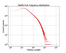
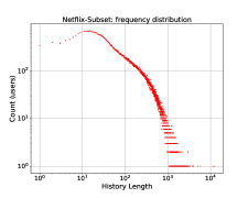
Figure 3. Comparison of the user distributions of the full Netflix dataset and the subsample produced by progressive stratified sampling.

5.2. Evaluation Metrics and protocol

Since we are considering implicit preferences, the evaluation is done on top-n recommendation, and it relies on the following metrics.

Normalized Discounted Cumulative Gain.:

Also abbreviated as NDCG@n, the metric gives more weight to the relevance of items on top of the recommender list and is defined as

$$\textit{NDCG@n}=\frac{\textit{DCG@n}}{\textit{IDCG@n}}$$

where

$$\textit{DCG@n}=\sum_{i=1}^{n}\frac{r_{i}}{log_{2}(i+1)}\quad\text{and}\quad\textit{IDCG@n}=\sum_{i=1}^{|\textit{R}|}\frac{1}{log_{2}(i+1)}.$$

Here, $r_{i}$ is the relevance (either 1 or 0 within the implicit feedback scenario) of the $i$-th recommended items in the recommendation list, and $R$ is the set of relevant items.

Precision.:

By defining $\textit{Hits}=\sum_{i}r_{i}$ as the number of items occurring in the recommendation list that were actually preferred by the user, we have

$$\vspace*{-1mm}\textit{Precision}@n=\frac{\textit{Hits}@n}{n}$$

Recall,:

defined as the percentage of items actually preferred by the user that were present in the recommendation list:

$$Recall@n=\frac{\textit{Hits}@n}{|R|}$$

In our experiments, we use the above metrics with two values of $n$, respectively $10$ and $100$.

The evaluation protocol works as follows. We partition users into training, validation and test set. The model is trained using the full histories of the users in the training set. During evaluation, for each user in the validation/test set we split the time-sorted user history into two parts, fold-in and fold-out splits. The fold-in split is used as a basis to learn the necessary representations and provide a recommendation list which is then evaluated with the fold-out split of the user history using the metrics defined above. We believe that this strategy is more robust when compared to other methodologies wherein the same user can be in both the training as well as testing sets. Table 1 shows the number of heldout users for each datasets.

It is worth noticing that Liang et. al (Liang et al., 2018) follow a similar strategy but with a major difference: they do not consider any sorting for user histories. That is, for the validation/test users, the fold-in set doesn’t precede the fold-out with respect to time. By contrast, we keep the fold-in set to be the first 80% of the time-sorted user history, and the last $20\%$ represents the fold-out set. We shall see in the following sections that this difference is substantial in the evaluation.

5.3. Competitors

We compare our model with various baselines and current state-of-the-art models including recently published neural architectures and we now present a brief summary about our competitors to provide a better understanding of these models.

• POP is a simple baseline where users are recommended the most popular items in the training set.

• BPR, already mentioned in section 4.2, is a state of the art model based on Matrix Factorization, which ranks items differently for each user (Rendle et al., 2009). There is a subtle issue concerning BPR: by separating users on training/validation/test as discussed above, the latent representation of users in the validation/test is not meaningful. That, is, BPR is only capable of providing meaningful predictions for users that were already exploited in the training phase. To solve this, we extended the training set to include the partial history in fold-in for each user in the validation/test. The evaluation still takes place on their corresponding fold-out sets.

• FPMC (Rendle et al., 2010) is a model which clubs both Matrix Factorization and Markov Chains together using personalized transition graphs over underlying Markov chains.

• CASER (Tang and Wang, 2018), already discussed in section 2, is a convolutional model that uses vertical and horizontal convolutional layers to embed a sequence of recent items thereby learning sequential patterns for next-item recommendation. The authors have shown that this model outperforms other approaches based on recurrent neural network modeling, such as GRU4Rec. We use the implementation provided by the authors and tune the network by keeping the number of horizontal filters to be 16, and vertical filters to be 4.

• MVAE, discussed in section 4.1, from which the SVAE model draws heavily. We use the implementation provided by the authors, with the default hyperparameter settings.

We also include the RVAE model proposed in section 4.2, that we consider a baseline here. Notably, despite being considered a simple extension of the BPR model, RVAE relies on a neural layer for embedding users: as a consequence, it does a better job in ranking items for the users which the model has never seen before, contrary to BPR. In practice, RVAE upgrades BPR to session-based recommendations.

5.4. Training Details

The experiments only consider the SVAE model illustrated in subsection 4.3.1 and the extensions of subsection 4.3.3. We reserve a more detailed analysis of the extensions discussed in subsection 4.3.2 to future work. The model is trained end-to-end on the full histories of the training users. Model hyperparameters are set using the evaluation metrics obtained on validation users.

The SVAE architecture includes an embedding layer of size 256, a recurrent layer realized as a GRU with 200 cells, and two encoding layers (of size 150 and 64) and finally two decoding layers (again, of size 64 and 150). We set the number $K$ of latent factors for the variational autoencoder to be 64. Adam (Kingma and Ba, 2014) was used to optimize the loss function coupled with a weight decay of $0.01$. As for RVAE, the architecture includes user/item embedding layers (of size 128), two encoding layers (size 100 and 64), and a final layer that produces the score $f_{\phi}(\bm{\mathit{z}}_{u,i})$. Both SVAE and RVAE were implemented in PyTorch (Paszke et al., 2017) and trained on a single GTX 1080Ti GPU. The source code is available on GitHub.

5.5. Results

Table 2. Results of the evaluation (in percentage). MVAE^∗ considers random splits that disregards the temporal order of user history. BPR^∗ relies on including the fold-in subsequences in the training phase.

In a first set of experiments, we compare SVAE with all competitors described above. Table 2 shows the results of the comparison. SVAE consistently outperforms the competitors on both datasets with a significant gain on all the metrics. It is important here to highlight how the temporal fold-in/fold-out split is crucial for a fair evaluation of the predictive capabilities: MVAE was evaluated both on temporal and random split, exhibiting totally different performances. Our interpretation is that, with random splits, the prediction for an item is easier if the encoding phase is aware of forthcoming items in the same user history. This severely affects the performance and overrates the predictive capabilities of a model: In fact, the accuracy of MVAE drops substantially when a temporal split is considered.

By contrast, SVAE is trained to capture the actual temporal dependencies and ultimately results in better predictive accuracy. This is also shown in fig. 4, where we show that SVAE consistently outperforms the competitors irrespective of the size of fold-in. The only exception is with very short sequences (less than 10 items), where MVAE gets better results with respect to the sequential models. It is also worth noticing how the performance of both sequential models tend to degrade with increasing sequences, but SVAE maintains its advantage over CASER.

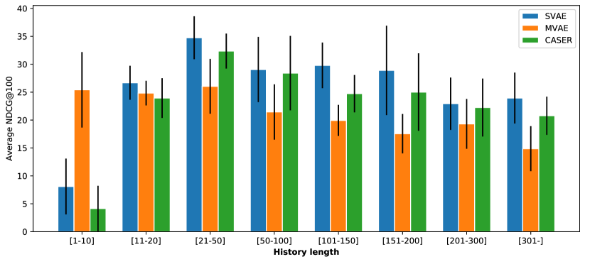
Figure 4. Average NDCG@100 for MVAE, CASER & SVAE across various history lengths.

We discussed in section 4.3.3 how the basic SVAE framework can be extended to focus on predicting the next $k$ items, rather then just the next item. We analyse this capability in fig. 5, where the accuracy for different values of $k$ is considered according to the modeling in 4.9. On Movielens, the best value is achieved for $k=4$, and acceptable values range within the interval $1-10$.

Figure 5. NDCG@100 values for SVAE on Movielens, across different sizes for the number of items forward in time to predict on.

Finally, in fig. 6 we analyse the convergence rate of SVAE, in terms of NDCG (left y-axis and blue line) and loss function values (right y-axis and red line). The learning phase converges quickly and does not exhibit overfitting: on Movielens, a stable model is reached within 8 epochs, whereas Netflix requires 13 epochs. The average runtime per epoch is 197 seconds on Movielens and 2 hours on Netflix: in practice, the learning scales linearly with the number of interactions in the dataset.

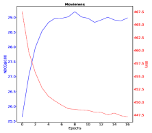
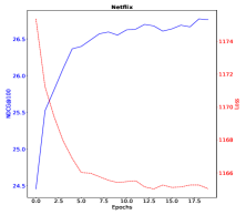
Figure 6. Learning curves on validation data.

6. Conclusions and future work

Combining the representation power of latent spaces, provided by variational autoencoders, with the sequence modeling capabilities of recurrent neural networks is an effective strategy to sequence recommendation. To prove this, we devised SVAE, a simple yet robust mathematical framework capable of modeling temporal dynamics upon different perspectives, within the fundamentals of variational autoencoders. The experimental evaluation highlights the capability of SVAE to consistently outperform state-of-the-art models.

The framework proposed here is worth further extensions that we plan to accomplish in a future work. From a conceptual point of view, we need to perform a thorough analysis of the taxonomy defined in section 4.3.2. From an architectural point of view, the attention mechanism, outlined in section 4.10, requires a better understanding and a more detailed analysis of its possible impact in view of the recent developments (Bahdanau et al., 2014) in the literature. Also, the SVAE framework relies on recurrent networks. However, different architectures (e.g. based on convolution (Tang and Wang, 2018) or translation invariance (He et al., 2017a)) are worth being investigated within a probabilistic variational setting.

References

- (1)
- Agarwal and Chen (2010) D. Agarwal and B. C. Chen. 2010. fLDA: Matrix Factorization Through Latent Dirichlet Allocation. In Proceedings of the Third ACM International Conference on Web Search and Data Mining (WSDM ’10). ACM, New York, NY, USA, 91–100.
- Aggarwal (2016) C. Aggarwal. 2016. Recommender Systems: The Textbook. Springer Publishing Company, Incorporated.
- Bahdanau et al. (2014) D. Bahdanau, K. Cho, and Y. Bengio. 2014. Neural Machine Translation by Jointly Learning to Align and Translate. CoRR abs/1409.0473 (2014).
- Barbieri and Manco (2011) N. Barbieri and G. Manco. 2011. An Analysis of Probabilistic Methods for Top-N Recommendation in Collaborative Filtering. In Proceedings of the Joint European Conference on Machine Learning and Knowledge Discovery in Databases (ECML/PKDD ’11). 172–187.
- Barbieri et al. (2014) N. Barbieri, G. Manco, and E. Ritacco. 2014. Probabilistic Approaches to Recommendations. Morgan & Claypool Publishers.
- Barbieri et al. (2013) N. Barbieri, G. Manco, E. Ritacco, M. Carnuccio, and A. Bevacqua. 2013. Probabilistic topic models for sequence data. Machine Learning (2013), 1–25.
- Bayer and Osendorfer (2014) J. Bayer and C. Osendorfer. 2014. Learning Stochastic Recurrent Networks. CoRR abs/1411.7610 (2014). http://arxiv.org/abs/1411.7610
- Blei et al. (2017) D. M. Blei, A. Kucukelbir, and J. D. McAuliffe. 2017. Variational Inference: A Review for Statisticians. J. Amer. Statist. Assoc. 112, 518 (2017), 859–877.
- Cho et al. (2014) K. Cho, B. van Merrienboer, Ç. Gülçehre, D. Bahdanau, F. Bougares, H. Schwenk, and Y. Bengio. 2014. Learning Phrase Representations using RNN Encoder-Decoder for Statistical Machine Translation. In Proceedings of the Conference on Empirical Methods in Natural Language Processing (EMNLP ’14). 1724–1734.
- Chung et al. (2014) J. Chung, Ç. Gülçehre, K. Cho, and Y. Bengio. 2014. Empirical Evaluation of Gated Recurrent Neural Networks on Sequence Modeling. CoRR abs/1412.3555 (2014). Presented at the Deep Learning workshop at NIPS2014.
- Chung et al. (2015) J. Chung, K. Kastner, L. Dinh, K. Goel, A. Courville, and Y. Bengio. 2015. A Recurrent Latent Variable Model for Sequential Data. In Proceedings of the 28th International Conference on Neural Information Processing Systems (NIPS’15). 2980–2988.
- Devooght and Bersini (2017) R. Devooght and H. Bersini. 2017. Long and Short-Term Recommendations with Recurrent Neural Networks. In Proceedings of the 25th Conference on User Modeling, Adaptation and Personalization (UMAP ’17). 13–21.
- Greff et al. (2017) K. Greff, R. K. Srivastava, J. Koutnik, B. R. Steunebrink, and J. Schmidhuber. 2017. LSTM: A Search Space Odyssey. IEEE Transactions on Neural Networks and Learning Systems 28, 10 (2017), 2222–2232.
- Gupta et al. (2018) K. Gupta, M. Yelahanka Raghuprasad, and P. Kumar. 2018. A Hybrid Variational Autoencoder for Collaborative Filtering. ArXiv e-prints (2018). arXiv:1808.01006
- He et al. (2017a) R. He, W. Kang, and J. McAuley. 2017a. Translation-based Recommendation. In Proceedings of the ACM Conference on Recommender Systems (RecSys ’17). 161–169.
- He and McAuley (2016) R. He and J. McAuley. 2016. Fusing Similarity Models with Markov Chains for Sparse Sequential Recommendation. In Proceedings of the IEEE 16th International Conference on Data Mining (ICDM ’16). 191–200.
- He et al. (2017b) X. He, L. Liao, H. Zhang, L. Nie, X. Hu, and T. Chua. 2017b. Neural Collaborative Filtering. In Proceedings of the 26th International Conference on World Wide Web (WWW ’17). 173–182.
- Hidasi et al. (2016) B. Hidasi, A. Karatzoglou, L. Baltrunas, and D. Tikk. 2016. Session-based Recommendations with Recurrent Neural Networks. In International Conference on Learning Representations (ICLR ’16).
- Hofmann (2004) T. Hofmann. 2004. Latent semantic models for collaborative filtering. ACM Transactions on Information Systems 22, 1 (2004), 89–115.
- Jannach and Ludewig (2017) D. Jannach and M. Ludewig. 2017. When Recurrent Neural Networks Meet the Neighborhood for Session-Based Recommendation. In Proceedings of the ACM Conference on Recommender Systems (RecSys ’17). 306–310.
- Kabbur et al. (2013) S. Kabbur, X. Ning, and G. Karypis. 2013. FISM: Factored Item Similarity Models for top-N Recommender Systems. In Proceedings of the 19th ACM SIGKDD International Conference on Knowledge Discovery and Data Mining (KDD ’13). 659–667.
- Kingma and Welling (2014) D.P. Kingma and M. Welling. 2014. Auto-Encoding Variational Bayes. In Proceedings of the 2nd International Conference on Learning Representations (ICLR ’14).
- Kingma and Ba (2014) D. P. Kingma and J. Ba. 2014. Adam: A Method for Stochastic Optimization. CoRR abs/1412.6980 (2014). http://arxiv.org/abs/1412.6980
- Koren (2008) Y. Koren. 2008. Factorization Meets the Neighborhood: A Multifaceted Collaborative Filtering Model. In Proceedings of the ACM SIGKDD International Conference on Knowledge Discovery and Data Mining (KDD ’08). 426–434.
- Li and She (2017) X. Li and J. She. 2017. Collaborative Variational Autoencoder for Recommender Systems. In Proceedings of the ACM SIGKDD International Conference on Knowledge Discovery and Data Mining (KDD ’17). 305–314.
- Liang et al. (2018) D. Liang, R. G. Krishnan, M.D. Hoffman, and T. Jebara. 2018. Variational Autoencoders for Collaborative Filtering. In Proceedings of the 2018 World Wide Web Conference (WWW ’18). 689–698.
- Liu et al. (2016) Q. Liu, S. Wu, D. Wang, Z. Li, and L. Wang. 2016. Context-Aware Sequential Recommendation. In Proceedings of the IEEE International Conference on Data Mining (ICDM ’16). 1053–1058.
- Murphy (2012) K. P. Murphy. 2012. Machine Learning: A Probabilistic Perspective. The MIT Press.
- Ning and Karypis (2011) X. Ning and G. Karypis. 2011. SLIM: Sparse Linear Methods for Top-N Recommender Systems. In Proceedings of the IEEE 11th International Conference on Data Mining (ICDM ’11). 497–506.
- Paszke et al. (2017) A. Paszke, S. Gross, S. Chintala, G. Chanan, E. Yang, Z. DeVito, Z. Lin, A. Desmaison, L. Antiga, and A. Lerer. 2017. Automatic differentiation in PyTorch. In NIPS Autodiff Workshop.
- Quadrana et al. (2018) M. Quadrana, P. Cremonesi, and D. Jannach. 2018. Sequence-Aware Recommender Systems. ACM Comput. Surv. 51, 4 (2018), 66:1–66:36.
- Quadrana et al. (2017) M. Quadrana, A. Karatzoglou, B. Hidasi, and P. Cremonesi. 2017. Personalizing Session-based Recommendations with Hierarchical Recurrent Neural Networks. In Proceedings of the ACM Conference on Recommender Systems (RecSys ’17). 130–137.
- Rendle (2012) S. Rendle. 2012. Factorization Machines with libFM. ACM Trans. Intell. Syst. Technol. 3, 3 (2012), 57:1–57:22.
- Rendle et al. (2009) S. Rendle, C. Freudenthaler, Z. Gantner, and L. Schmidt-Thieme. 2009. BPR: Bayesian Personalized Ranking from Implicit Feedback. In Proceedings of the Twenty-Fifth Conference on Uncertainty in Artificial Intelligence (UAI ’09). 452–461.
- Rendle et al. (2010) S. Rendle, C. Freudenthaler, and L. Schmidt-Thieme. 2010. Factorizing Personalized Markov Chains for Next-basket Recommendation. In Proceedings of the International Conference on World Wide Web (WWW ’10). 811–820.
- Rezende et al. (2014) D. J. Rezende, S. Mohamed, and D. Wierstra. 2014. Stochastic Backpropagation and Approximate Inference in Deep Generative Models. In Proceedings of the 31th International Conference on Machine Learning (ICML ’14). 1278–1286.
- Rifai et al. (2011) S. Rifai, P Vincent, X. Muller, X. Glorot, and Y. Bengio. 2011. Contractive Auto-encoders: Explicit Invariance During Feature Extraction. In Proceedings of the International Conference on International Conference on Machine Learning (ICML’11). 833–840.
- Salakhutdinov and Mnih (2008a) R. Salakhutdinov and A. Mnih. 2008a. Bayesian Probabilistic Matrix Factorization Using Markov Chain Monte Carlo. In Proceedings of the International Conference on Machine Learning (ICML ’08). 880–887.
- Salakhutdinov and Mnih (2008b) R. Salakhutdinov and A. Mnih. 2008b. Probabilistic Matrix Factorization. In Proceedings of the International Conference on Neural Information Processing Systems (NIPS ’08). 1257–1264.
- Sedhain et al. (2015) S. Sedhain, A. K. Menon, S. Sanner, and L. Xie. 2015. AutoRec: Autoencoders Meet Collaborative Filtering. In Proceedings of the International Conference on World Wide Web (WWW ’15). 111–112.
- Strub and Mary (2015) F. Strub and J. Mary. 2015. Collaborative Filtering with Stacked Denoising AutoEncoders and Sparse Inputs. In NIPS Workshop on Machine Learning for eCommerce. https://hal.inria.fr/hal-01256422
- Tan et al. (2016) Y. K. Tan, X. Xu, and Y. Liu. 2016. Improved Recurrent Neural Networks for Session-based Recommendations. In Proceedings of the 1st Workshop on Deep Learning for Recommender Systems (DLRS ’16). 17–22.
- Tang and Wang (2018) J. Tang and K. Wang. 2018. Personalized Top-N Sequential Recommendation via Convolutional Sequence Embedding. In Proceedings of the ACM International Conference on Web Search and Data Mining (WSDM ’18). 565–573.
- Tavakol and Brefeld (2014) M. Tavakol and U. Brefeld. 2014. Factored MDPs for Detecting Topics of User Sessions. In Proceedings of the 8th ACM Conference on Recommender Systems (RecSys ’14). 33–40.
- Twardowski (2016) B. Twardowski. 2016. Modelling Contextual Information in Session-Aware Recommender Systems with Neural Networks. In Proceedings of the ACM Conference on Recommender Systems (RecSys ’16). 273–276.
- Vaswani et al. (2017) A. Vaswani, N. Shazeer, N. Parmar, J. Uszkoreit, L. Jones, A. N Gomez, L. Kaiser, and I Polosukhin. 2017. Attention is All you Need. In Advances in Neural Information Processing Systems 30. 5998–6008.
- Vincent et al. (2010) P. Vincent, H. Larochelle, I. Lajoie, Y. Bengio, and P. A. Manzagol. 2010. Stacked Denoising Autoencoders: Learning Useful Representations in a Deep Network with a Local Denoising Criterion. J. Mach. Learn. Res. 11 (2010).
- Wang and Blei (2011) C. Wang and D. Blei. 2011. Collaborative Topic Modeling for Recommending Scientific Articles. In Proceedings of the 17th ACM SIGKDD International Conference on Knowledge Discovery and Data Mining (KDD ’11). 448–456.
- Wang et al. (2015) H. Wang, N. Wang, and D. Y. Yeung. 2015. Collaborative Deep Learning for Recommender Systems. In Proceedings of the ACM SIGKDD International Conference on Knowledge Discovery and Data Mining (KDD ’15). 1235–1244.
- Wu et al. (2017) C. Wu, A. Ahmed, A. Beutel, and H. Smola, A.and Jing. 2017. Recurrent Recommender Networks. In Proceedings of the ACM International Conference on Web Search and Data Mining (WSDM ’17). 495–503.
- Wu et al. (2016) S. Wu, W. Ren, C. Yu, G. Chen, D. Zhang, and J. Zhu. 2016. Personal recommendation using deep recurrent neural networks in NetEase. In Proceedings of the IEEE International Conference on Data Engineering (ICDE ’16). 1218–1229.
- Zhang et al. (2017a) S. Zhang, L. Yao, and A. Sun. 2017a. Deep Learning based Recommender System: A Survey and New Perspectives. CoRR abs/1707.07435 (2017). http://arxiv.org/abs/1707.07435
- Zhang et al. (2017b) S. Zhang, L. Yao, and X. Xu. 2017b. AutoSVD++: An Efficient Hybrid Collaborative Filtering Model via Contractive Auto-encoders. In Proceedings of the International ACM SIGIR Conference on Research and Development in Information Retrieval (SIGIR ’17). 957–960.