Projections for model-independent sensitivity estimates on top-quark anomalous electromagnetic couplings at the FCC-he

Abstract

The measurement of the top-quark anomalous electromagnetic couplings is one of the most important goals of the top-quark physics program in present and future collider experiments and would provide direct information on the non-standard interactions of the top-quark. We study a top-quark pair production scenario at the Future Circular Collider Hadron-Electron (FCC-he) through $e^{-}p\to e^{-}\gamma^{*}\gamma^{*}p\to e^{-}t\bar{t}p$ collisions, which will provide information on the sensitivities of anomalous $\hat{a}_{V}$ and $\hat{a}_{A}$ couplings at $95\%\hskip 2.27621ptC.L.$, as well as create the possibility of probing new physics. Energy of the $e^{-}$ beams is taken to be $E_{e}=250\hskip 2.27621ptGeV$ and $500\hskip 2.27621ptGeV$, and the energy of the $p$ beams is considered to be $E_{p}=50\hskip 2.27621ptTeV$. With these energies the FCC-he can measure the dipole moments of the top-quark $\hat{a}_{V}$ and $\hat{a}_{A}$ with a sensitivity of the order ${\cal O}(10^{-2}-10^{-1})$.

I Introduction

The detection of the Higgs boson Tanabashi ; Englert ; Higgs ; Higgs1 ; Guralnik by the ATLAS Atlas and CMS CMS Collaborations at the Large Hadron Collider (LHC), together with the absence so far of any signature new physics beyond the Standard Model (BSM) in collisions at center-of-mass energies of several $TeV$, has triggered great interest of the scientific community in the planning of future colliders that increase the energy and precision frontiers in cleaner environments. The Future Circular Collider (FCC) study develops options for potential high-energy frontier circular colliders at CERN for the post LHC era that will open up new horizons in the field of fundamental physics. These colliders, with their high precision and high-energy reach, could extend the search for new particles and interactions well beyond the LHC that may hold the key to understanding and responding to the open problems of the SM such as: evidence for dark matter, prevalence of matter over antimatter, and neutrino masses. The FCC study puts great emphasis on the scenarios of high-intensity and high-energy frontier colliders: $pp$, $e^{+}e^{-}$ and $e^{-}p$. It should be mentioned that in comparison with the LHC, the FCC-he has the advantage of providing a clean environment with small background contributions from QCD strong interactions. In addition, as the initial states are asymmetric, the backward and forward scattering can be disentangled.

In this paper we considered the electron-proton collision of the FCC-he that is proposed to build on the same site with LHC, as the future extension of the Large Hadron Electron Collider (LHeC). In FCC-he, construction of an Energy Recovery Linac (ERL) is proposed to deliver electrons with energies ranging from $E_{e}=250\hskip 2.27621pt{\rm GeV}$ to $E_{e}=500\hskip 2.27621pt{\rm GeV}$, while a proton beam is provided by the main FCC ring based on a new $80-100\hskip 2.27621pt{\rm km}$ circumference tunnel infrastructure. The FCC-eh will collide a $250\hskip 2.27621pt{\rm GeV}$ to $500\hskip 2.27621pt{\rm GeV}$ electron beam from a linear accelerator external and tangential to the main FCC tunnel, with a $50\hskip 2.27621pt{\rm TeV}$ proton beam. In addition, it would collect factors of thousands more luminosity than the first colliders electron-proton such as the Hadron-Electron Ring Accelerator (HERA). The machine would serve as the most powerful, high-resolution microscope onto the substructure of matter ever built. High-energy $ep$ collisions would provide precise information on the quark and gluon structure of the proton, and how they interact. This machine would complement and enhance the study of the physics of the Higgs boson, top-quark, tau-lepton and broaden the new physics searches also performed at the Future Circular Collider Hadron-Hadron (FCC-hh) and the Future Circular Collider Electro-Electron (FCC-ee). Discoveries such as quark substructure might also arise. In $ep$ collisions new particles can be created in the annihilation of the electron and a (anti)quark, or may be radiated in the exchange of a photon or other vector bosons. FCC-eh could also provide access to Higgs self-interactions and extended Higgs sectors, including scenarios involving dark matter. If neutrino oscillations arise from the existence of heavy sterile neutrinos, direct searches at the FCC-eh would have great discovery prospects in kinematic regions complementary to FCC-hh and FCC-ee, giving the FCC complex a striking potential to shine light on the origin of neutrino masses. For a complete and detailed study on the physics and detector design concepts see Refs. FCChe ; Fernandez ; Fernandez1 ; Fernandez2 ; Huan ; Acar .

The aim of this study is to obtain model-independent sensitivity estimates on top-quark anomalous electromagnetic couplings $\tilde{a}_{V}$ and $\tilde{a}_{A}$ at the Future Circular Collider Hadron-Electron (FCC-he) FCChe ; Fernandez ; Fernandez1 ; Fernandez2 ; Huan ; Acar ; Bruening through $e^{-}p\to e^{-}\gamma^{*}\gamma^{*}p\to e^{-}t\bar{t}p$ collisions. We have based our study on the FCC-he which has been designed to collide electrons with an energy $E_{e}=250\hskip 2.27621ptGeV$ to $E_{e}=500\hskip 2.27621ptGeV$ with protons with an energy $E_{p}=50\hskip 2.27621ptTeV$, corresponding to the center-of-mass energies $\sqrt{s}=2\sqrt{E_{e}E_{p}}=7.07\hskip 2.27621ptTeV$ and $10\hskip 2.27621ptTeV$. Depending on the energy of the incoming electrons and the design of the collider, the anticipated integrated luminosity is approximately $50-1000\hskip 2.27621ptfb^{-1}$.

Many studies on the physical potential of top-quark using different processes and environments have been presented by several theoretical, experimental and phenomenological authors and groups. Furthermore, the processes involving top-quarks provide us unique opportunities to test the Standard Model (SM) predictions and look for possible signatures of new physics BSM. These signals can be the anomalous electromagnetic dipole moments of the top-quark, that is, its Magnetic Moment ($t$-MM) and its Electric Dipole Moment ($t$-EDM), with the latter considered as a source of CP violation. The estimate in the SM for the $t$-MM $(a_{t})$ Benreuther and $t$-EDM $(d_{t})$ Hoogeveen ; Pospelov ; Soni is given by:

$$\mbox{SM}:\begin{array}[]{ll}a_{t}=0.02,\\ d_{t}<10^{-30}(ecm),\end{array}$$ (1)

and the $t$-MM can be tested in the LHC and future colliders such as the Compact Linear Collider (CLIC), the Large Hadron-Electron Collider (LHeC) and the FCC-he. As shown in Eq. (1), the $t$-EDM value is strongly suppressed and difficult to measure. What’s more, if its value were zero, it wouldn’t be possible to measure it at all. However, the $t$-EDM is very useful for probing new physics BSM.

A summary of sensitivities achievable on the electromagnetic dipole moments of the top-quark is given in Table I. See Refs. Ibrahim ; Atwood ; Polouse ; Choi ; Polouse1 ; Aguilar0 ; Amjad ; Juste ; Asner ; Abe ; Aarons ; Brau ; Baer ; Grzadkowski:2005ye for other results on the $t$-MM and the $t$-EDM in different contexts.

Table 1: Summary of sensitivities achievable on the electromagnetic dipole moments of the top-quark.

Model	Theoretical sensitivity: $\hat{a}_{V}$, $\hat{a}_{A}$	C. L.	Reference
Top-quark pair production at LHC	$(-0.041,0.043),(-0.035,0.038)$	$68\%$	Juste
$t\bar{t}\gamma$ production at LHC	$(-0.2,0.2),(-0.1,0.1)$	$90\%$	Baur
Radiative $b\to s\gamma$ transitions at Tevatron and LHC	$(-2,0.3),(-0.5,1.5)$	$90\%$	Bouzas
Process $pp\to p\gamma^{*}\gamma^{*}p\to pt\bar{t}p$ at LHC	$(-0.6389,0.0233),(-0.1158,0.1158)$	$68\%$	Sh
Measurements of $\gamma p\to t\bar{t}$ at LHeC	$(-0.05,0.05),(-0.20,0.20)$	$90\%$	Bouzas1
Top-quark pair production $e^{+}e^{-}\to t\bar{t}$ at ILC	$(-0.002,0.002),(-0.001,0.001)$	$68\%$	Aguilar
Process $\gamma e^{-}\to\bar{t}b\nu_{e}$ at CLIC	$(-0.0258,0.0350),(-0.0301,0.0301)$	$95\%$	murat
Process $e^{+}e^{-}\to e^{+}\gamma^{*}e^{-}\to\bar{t}b\nu_{e}e^{+}$ at CLIC	$(-0.0609,0.1081),(-0.0777,0.0777)$	$95\%$	murat
Mode $\gamma\gamma\to t\bar{t}$ at CLIC	$(-0.02203,0.0020),(-0.0206,0.0206)$	$95\%$	Billur
Mode $e^{+}\gamma\to e^{+}\gamma^{*}\gamma\to e^{+}t\bar{t}$ at CLIC	$(-0.4570,0.0045),(-0.0431,0.0431)$	$95\%$	Billur
Mode $e^{+}e^{-}\to e^{+}\gamma^{*}\gamma^{*}e^{-}\to e^{+}t\bar{t}e^{-}$ at CLIC	$(-0.6013,0.0151),(-0.0890,0.0890)$	$95\%$	Billur

The structure of this paper is as follows. In Section II, we introduce the top-quark effective electromagnetic interactions. In Section III, we present sensitivity estimates on top-quark anomalous electromagnetic couplings through $e^{-}p\to e^{-}\gamma^{*}\gamma^{*}p\to e^{-}t\bar{t}p$ collisions. In Section IV, we present our conclusions .

II Production of $t\bar{t}$ pairs via the process $e^{-}p\to e^{-}\gamma^{*}\gamma^{*}p\to e^{-}t\bar{t}p$

II.1 Top-quark Effective Coupling $t\bar{t}\gamma$

A suitable model-independent formalism for describing possible new physics effects is based on effective Lagrangian. In this formalism, all the heavy degrees of freedom are integrated out to obtain the effective interactions between the SM particles. This is justified due to the fact that the related observables have so far not shown any significant deviation from the SM predictions. In the effective Lagrangian formalism, potential deviations from the SM for the anomalous $t\bar{t}\gamma$ coupling could be described using the following Lagrangian:

$${\cal L}_{eff}={\cal L}_{SM}+\sum_{n}\frac{\alpha_{n}}{\Lambda^{2}}{\cal O}^{(6)}_{n}+h.c..$$ (2)

Here, ${\cal L}_{eff}$ is the effective Lagrangian which contains a series of higher-dimensional operators built with the SM fields, ${\cal L}_{SM}$ is the renormalizable SM Lagrangian, $\Lambda$ is the scale at which new physics is expected to be observed, $\alpha_{n}$ are dimensionless coefficients and ${\cal O}^{(6)}_{n}$ represents the dimension-six gauge-invariant operator.

The most general effective coupling $t\bar{t}\gamma$ includes the SM coupling and contributions from dimension-six effective operators and can be written as Sh ; Kamenik ; Baur ; Aguilar ; Aguilar1 :

$${\cal L}_{t\bar{t}\gamma}=-g_{e}Q_{t}\bar{t}\Gamma^{\mu}_{t\bar{t}\gamma}tA_{\mu},$$ (3)

where $g_{e}$ is the electromagnetic coupling constant, and $Q_{t}$ is the top-quark electric charge. The Lorentz-invariant vertex function $\Gamma^{\mu}_{t\bar{t}\gamma}$, which describes the interaction of a $\gamma$ photon with two top-quarks, can be parameterized by:

$$\Gamma^{\mu}_{t\bar{t}\gamma}=\gamma^{\mu}+\frac{i}{2m_{t}}(\hat{a}_{V}+i\hat{a}_{A}\gamma_{5})\sigma^{\mu\nu}q_{\nu},$$ (4)

where $m_{t}$ is the mass of the top-quark, $q$ is the momentum transfer to the photon, and the couplings $\hat{a}_{V}$ and $\hat{a}_{A}$ are real and related to the anomalous magnetic moment $(a_{t})$ and the electric dipole moment $(d_{t})$ of the top-quark, respectively. The relations between $\hat{a}_{V}(\hat{a}_{A})$ and $a_{t}(d_{t})$ are given by:

$$\hat{a}_{V} = Q_{t}a_{t},$$ (5)

$$\hat{a}_{A} = \frac{2m_{t}}{e}d_{t}.$$ (6)

The operators that contribute to top-quark eletromagnetic anomalous couplings Buhmuller ; Aguilar2 are:

$${\cal O}_{uW}^{33}=\bar{q}_{L3}\sigma^{\mu\nu}\tau^{a}t_{R}{\tilde{\phi}}W_{\mu\nu}^{a},$$ (7)

$${\cal O}_{uB\phi}^{33}=\bar{q}_{L3}\sigma^{\mu\nu}t_{R}{\tilde{\phi}}B_{\mu\nu},$$ (8)

where $\bar{q}_{L3}$ is the quark field, $\sigma^{\mu\nu}$ are the Pauli matrices and ${\tilde{\phi}}$ is the Higgs doublet, while $W_{\mu\nu}^{a}$ and $B_{\mu\nu}$ are the $U(1)_{Y}$ and $SU(2)_{L}$ gauge field strength tensors, respectively.

From the parametrization given by Eq. (3), and from the operators of dimension-six given in Eqs. (7) and (8) we obtain the corresponding CP even ${\hat{a}_{V}}$ and CP odd ${\hat{a}_{A}}$ observables:

$$\hat{a}_{V}=\frac{2m_{t}}{e}\frac{\sqrt{2}\upsilon}{\Lambda^{2}}Re\Bigl{[}\cos\theta_{W}C_{uB\phi}^{33}+\sin\theta_{W}C_{uW}^{33}\Bigr{]},$$ (9)

$$\hat{a}_{A}=\frac{2m_{\tau}}{e}\frac{\sqrt{2}\upsilon}{\Lambda^{2}}Im\Bigl{[}\cos\theta_{W}C_{uB\phi}^{33}+\sin\theta_{W}C_{uW}^{33}\Bigr{]}.$$ (10)

In these equations, $\upsilon=246$ GeV is the breaking scale of the electroweak symmetry, $\Lambda$ is the new physics scale, and $\sin\theta_{W}(\cos\theta_{W})$ is the sine(cosine) of the weak mixing angle.

II.2 Theoretical Calculations

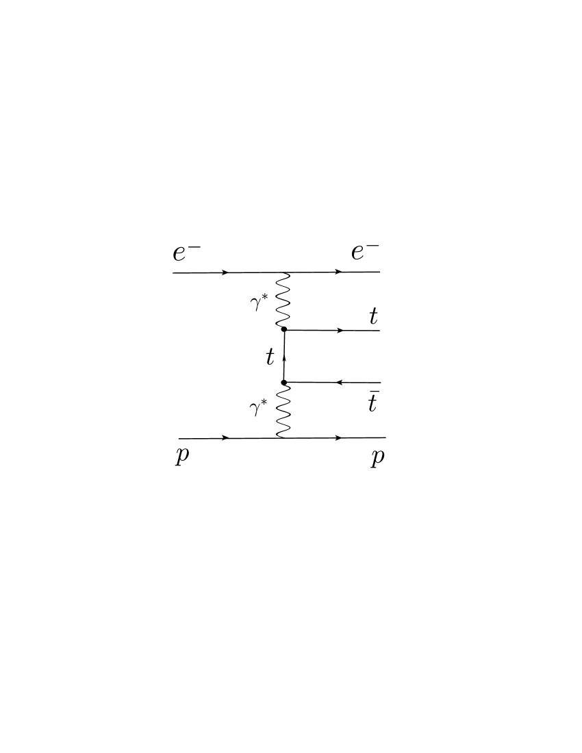
Figure 1: A schematic diagram for the process $e^{-}p\to e^{-}\gamma^{*}\gamma^{*}p\to e^{-}t\bar{t}p$.

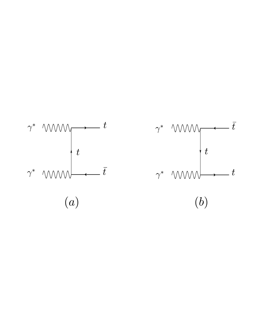
Figure 2: Feynman diagrams contributing to the subprocess $\gamma^{*}\gamma^{*}\to t\bar{t}$.

In the $e^{-}p$ colliders, the top-quark pairs can be produced through the channel $e^{-}p\to e^{-}\gamma^{*}\gamma^{*}p\to e^{-}t\bar{t}p$. The schematic diagram corresponding to this process is given in Fig. 1. The representative leading order Feynman diagrams for the subprocess $\gamma^{*}\gamma^{*}\to t\bar{t}$ are depicted in Fig. 2.

For the $\gamma^{*}\gamma^{*}$ collision, including the effects of the effective Lagrangian given by Eq. (3), the corresponding matrix elements for the subprocess $\gamma^{*}\gamma^{*}\to t\bar{t}$ are given as a function of the Mandelstam invariants $\hat{s}$, $\hat{t}$ and $\hat{u}$, as well as of their dipole moments $\hat{a}_{V}$ and $\hat{a}_{A}$:

$$|M_{1}|^{2} = \frac{16\pi^{2}Q_{t}^{2}\alpha^{2}_{e}}{2m_{t}^{4}(\hat{t}-m_{t}^{2})^{2}}\biggl{[}48\hat{a}_{V}(m_{t}^{2}-\hat{t})(m_{t}^{2}+\hat{s}-\hat{t})m_{t}^{4}-16(3m_{t}^{4}-m_{t}^{2}\hat{s}+\hat{t}(\hat{s}+\hat{t}))m_{t}^{4}$$ (11)

$$+ 2(m_{t}^{2}-\hat{t})(\hat{a}_{V}^{2}(17m_{t}^{4}+(22\hat{s}-26\hat{t})m_{t}^{2}+\hat{t}(9\hat{t}-4\hat{s}))$$

$$+ \hat{a}_{A}^{2}(17m_{t}^{2}+4\hat{s}-9\hat{t})(m_{t}^{2}-\hat{t}))m_{t}^{2}+12\hat{a}_{V}(\hat{a}_{V}^{2}+\hat{a}_{A}^{2})\hat{s}(m_{t}^{3}-m_{t}\hat{t})^{2}$$

$$- (\hat{a}_{V}^{2}+\hat{a}_{A}^{2})^{2}(m_{t}^{2}-\hat{t})^{3}(m_{t}^{2}-\hat{s}-\hat{t})\biggr{]},$$

$$|M_{2}|^{2} = \frac{-16\pi^{2}Q_{t}^{2}\alpha^{2}_{e}}{2m_{t}^{4}(\hat{u}-m_{t}^{2})^{2}}\biggl{[}48\hat{a}_{V}(m_{t}^{4}+(\hat{s}-2\hat{t})m_{t}^{2}+\hat{t}(\hat{s}+\hat{t}))m_{t}^{4}$$ (12)

$$+ 16(7m_{t}^{4}-(3\hat{s}+4\hat{t})m_{t}^{2}+\hat{t}(\hat{s}+\hat{t}))m_{t}^{4}$$

$$+ 2(m_{t}^{2}-\hat{t})(\hat{a}_{V}^{2}(m_{t}^{4}+(17\hat{s}-10\hat{t})m_{t}^{2}+9\hat{t}(\hat{s}+\hat{t}))$$

$$+ \hat{a}_{A}^{2}(m_{t}^{2}-9\hat{t})(m_{t}^{2}-\hat{t}-\hat{s}))m_{t}^{2}$$

$$+ (\hat{a}_{V}^{2}+\hat{a}_{A}^{2})^{2}(m_{t}^{2}-\hat{t})^{3}(m_{t}^{2}-\hat{s}-\hat{t})\biggr{]},$$

$$M_{1}^{{\dagger}}M_{2}+M_{2}^{{\dagger}}M_{1} = \frac{16\pi^{2}Q_{t}^{2}\alpha^{2}_{e}}{m_{t}^{2}(\hat{t}-m_{t}^{2})(\hat{u}-m_{t}^{2})}$$ (13)

$$\times \biggl{[}-16(4m_{t}^{6}-m_{t}^{4}\hat{s})+8\hat{a}_{V}m_{t}^{2}(6m_{t}^{4}-6m_{t}^{2}(\hat{s}+2\hat{t})-\hat{s})^{2}$$

$$+ 6\hat{t})^{2}+6\hat{s}\hat{t})+(\hat{a}_{V}^{2}(16m_{t}^{6}-m_{t}^{4}(15\hat{s}+32\hat{t})+m_{t}^{2}(15\hat{s})^{2}$$

$$+ 14\hat{t}\hat{s}+16\hat{t})^{2})+\hat{s}\hat{t}(\hat{s}+\hat{t}))+\hat{a}_{A}^{2}(16m_{t}^{6}-m_{t}^{4}(15\hat{s}+32\hat{t})$$

$$+ m_{t}^{2}(5\hat{s})^{2}+14\hat{t}\hat{s}+16\hat{t})^{2})+\hat{s}\hat{t}(\hat{s}+\hat{t})))-4\hat{a}_{V}\hat{s}(\hat{a}_{V}^{2}+\hat{a}_{A}^{2})$$

$$\times (m_{t}^{4}+m_{t}^{2}(\hat{s}-2\hat{t})+\hat{t}(\hat{s}+\hat{t}))-4\hat{a}_{A}(\hat{a}_{V}^{2}+\hat{a}_{A}^{2})(2m_{t}^{2}-\hat{s}-2\hat{t})$$

$$\times \epsilon_{\alpha\beta\gamma\delta}p_{1}^{\alpha}p_{2}^{\beta}p_{3}^{\gamma}p_{4}^{\delta}-2\hat{s}(\hat{a}_{V}^{2}+\hat{a}_{A}^{2})^{2}(m_{t}^{4}-2\hat{t}m_{t}^{2}+\hat{t}(\hat{s}+\hat{t}))\biggr{]}.$$

In Eqs. (11)-(13), $\hat{s}=(p_{1}+p_{2})^{2}=(p_{3}+p_{4})^{2}$, $\hat{t}=(p_{1}-p_{3})^{2}=(p_{4}-p_{2})^{2}$, $\hat{u}=(p_{3}-p_{2})^{2}=(p_{1}-p_{4})^{2}$, where $p_{1}$ and $p_{2}$ are the four-momenta of the incoming photons, $p_{3}$ and $p_{4}$ are the momenta of the outgoing top-quarks, $Q_{t}$ is the top-quark charge, $\alpha_{e}=g^{2}_{e}/4\pi$ is the fine-structure constant and $m_{t}$ is the mass of the top-quark.

The Weizsacker-Williams Approximation (WWA), also alternatively called the Equivalent Photon Approximation (EPA) Budnev ; Baur1 ; Piotrzkowski , is useful for determining the $e^{-}p\to e^{-}\gamma^{*}\gamma^{*}p\to e^{-}t\bar{t}p$ scattering cross-section. In EPA, photons emitted from incoming charged particles with very low virtuality are scattered at very small angles from the beam pipe. Because the emitted quasi-real photons have a low $Q^{2}$ virtuality, they are almost real. These processes have been observed experimentally at the LEP, the Tevatron and the LHC Abulencia ; Aaltonen1 ; Aaltonen2 ; Chatrchyan1 ; Chatrchyan2 ; Abazov ; Chatrchyan3 . In WWA or EPA, the quasi-real photons emitted from both lepton and proton beams collide with each other and produce the subprocess $\gamma^{*}\gamma^{*}\rightarrow t\bar{t}$. In the WWA, the spectrum of the photon emitted by electron $(\gamma^{*}_{1})$ is given by Belyaev ; Budnev :

$$f_{\gamma^{*}_{1}}(x_{1}) = \frac{\alpha}{\pi E_{e}}\left\{\left[\frac{1-x_{1}+x_{1}^{2}/2}{x_{1}}\right]\log{\left(\frac{Q_{max}^{2}}{Q_{min}^{2}}\right)}-\frac{m_{e}^{2}x_{1}}{Q_{min}^{2}}\left(1-\frac{Q_{min}^{2}}{Q_{max}^{2}}\right)\right.$$

$$- \left.\frac{1}{x_{1}}\left[1-\frac{x_{1}}{2}\right]^{2}log\left(\frac{x_{1}^{2}E_{e}^{2}+Q_{max}^{2}}{x_{1}^{2}E_{e}^{2}+Q_{min}^{2}}\right)\right\},$$

where $x_{1}=E_{\gamma^{*}_{1}}/E_{e}$ and $Q^{2}_{max}$ is maximum virtuality of the photon. The minimum value of the $Q^{2}_{min}$ is given by:

$$Q_{min}^{2}=\frac{m_{e}^{2}x_{1}^{2}}{1-x_{1}}.$$ (15)

The spectrum of the photon emitted by proton $(\gamma^{*}_{2})$ can be written as follows Belyaev ; Budnev :

$$f_{\gamma^{*}_{2}}(x_{2})=\frac{\alpha}{\pi E_{p}}\left\{\left[1-x_{2}\right]\left[\varphi\left(\frac{Q_{max}^{2}}{Q_{0}^{2}}\right)-\varphi\left(\frac{Q_{min}^{2}}{Q_{0}^{2}}\right)\right]\right\},$$ (16)

where the function $\varphi$ is given by:

$$\varphi(\theta)= (1+ay)\left[-\textit{In}\left(1+\frac{1}{\theta}\right)+\sum_{k=1}^{3}\frac{1}{k(1+\theta)^{k}}\right]+\frac{y(1-b)}{4\theta(1+\theta)^{3}}$$ (17)

$$+c(1+\frac{y}{4})\left[\textit{In}\left(\frac{1-b+\theta}{1+\theta}\right)+\sum_{k=1}^{3}\frac{b^{k}}{k(1+\theta)^{k}}\right].$$

From Eq. (17), we define the following:

$$y=\frac{x_{2}^{2}}{(1-x_{2})},$$ (18)

$$a=\frac{1+\mu_{p}^{2}}{4}+\frac{4m_{p}^{2}}{Q_{0}^{2}}\approx 7.16,$$ (19)

$$b=1-\frac{4m_{p}^{2}}{Q_{0}^{2}}\approx-3.96,$$ (20)

$$c=\frac{\mu_{p}^{2}-1}{b^{4}}\approx 0.028.$$ (21)

Therefore, the total cross-section of the $e^{-}p\to e^{-}\gamma^{*}\gamma^{*}p\to e^{-}t\bar{t}p$ signal in the WWA is obtained as follows:

$$\sigma(e^{-}p\rightarrow e^{-}\gamma^{*}\gamma^{*}p\rightarrow e^{-}t\bar{t}p)=\int_{x_{1}^{min}}^{x_{1}^{max}}\int_{x_{2}^{min}}^{x_{2}^{max}}f_{\gamma_{1}^{*}}(x_{1})f_{\gamma_{2}^{*}}(x_{2})d\hat{\sigma}(\gamma^{*}\gamma^{*}\rightarrow t\bar{t})dx_{1}dx_{2}.$$ (22)

The main anomalous electromagnetic couplings affecting top-quark physics that are of interest for our study are $\hat{a}_{V}$ and $\hat{a}_{A}$. We calculate the dependencies of the $e^{-}p\to e^{-}\gamma^{*}\gamma^{*}p\to e^{-}t\bar{t}p$ associated production cross-sections for FCC-he at $7.07\hskip 2.27621ptTeV$ and $10\hskip 2.27621ptTeV$ on $\hat{a}_{V}$ and $\hat{a}_{A}$ using CalcHEP Belyaev , obtaining the following numerical results:

$i)$ For $\sqrt{s}=7.07\hskip 2.27621ptTeV$.

$$\sigma(\hat{a}_{V}) = \Bigl{[}(0.00458)\hat{a}_{V}^{4}+(0.00829)\hat{a}^{3}_{V}+(0.01158)\hat{a}^{2}_{V}+(0.00439)\hat{a}_{V}+0.00165\Bigr{]}(pb)$$ (23)

$$\sigma(\hat{a}_{A}) = \Bigl{[}(0.00458)\hat{a}_{A}^{4}+(0.00937)\hat{a}^{2}_{A}+0.00165\Bigr{]}(pb).$$ (24)

$ii)$ For $\sqrt{s}=10\hskip 2.27621ptTeV$.

$$\sigma(\hat{a}_{V}) = \Bigl{[}(0.00928)\hat{a}_{V}^{4}+(0.01263)\hat{a}^{3}_{V}+(0.01712)\hat{a}^{2}_{V}+(0.00596)\hat{a}_{V}+0.00225\Bigr{]}(pb)$$ (25)

$$\sigma(\hat{a}_{A}) = \Bigl{[}(0.00928)\hat{a}_{A}^{4}+(0.01414)\hat{a}^{2}_{A}+0.00225\Bigr{]}(pb).$$ (26)

The sensitivities on the total cross-section and on the coefficients of $\hat{a}_{V}$ and $\hat{a}_{A}$ increase with the center-of-mass energy, confirming the expected competitive advantage of the high-energies attainable with the FCC-he.

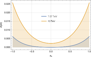
Figure 4: Same as in Fig. 3, but for $\hat{a}_{A}$.

For signal production, as shown in Figs. 3 and 4, we give the total cross-section of the process $e^{-}p\to e^{-}\gamma^{*}\gamma^{*}p\to e^{-}t\bar{t}p$ as a function of the anomalous couplings $\hat{a}_{V}$ and $\hat{a}_{A}$ corresponding to the effective vertex $t\bar{t}\gamma$. We maintain the energy of the $e^{-}p$ collider at $\sqrt{s}=7.07\hskip 2.27621ptTeV$ and $\sqrt{s}=10\hskip 2.27621ptTeV$, the two main options of FCC-he.

As shown in Figs. 3 and 4, the anomalous $\hat{a}_{V}$ and $\hat{a}_{A}$ parameters have different CP properties which can be seen in Eqs. (11)-(13) and in Eqs. (23)-(26). The contribution of $\hat{a}_{V}$ coupling to the total cross-section is proportional to even and odd powers. In Fig. 3, there are small intervals around $\hat{a}_{V}$ in which the cross-section that includes new physics is smaller than the SM cross-section (from Eqs. (23) and (25), terms depending on $\hat{a}_{V}$ give purely the contribution BSM, and those which do not dependent on $\hat{a}_{V}$ give the SM cross-section). For this reason, the $\hat{a}_{V}$ coupling has a partially destructive effect on the total cross-section. Furthermore, in Fig. 4 the total cross-section with respect to the $\hat{a}_{A}$ parameter is of even power and a nonzero value of this parameter allows a constructive effect on the total cross-section.

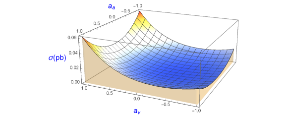
Figure 5: The total cross sections of the process $e^{-}p\to e^{-}\gamma^{*}\gamma^{*}p\to e^{-}t\bar{t}p$ as a function of $\hat{a}_{V}$ and $\hat{a}_{A}$ for center-of-mass energy of $\sqrt{s}=7.07$ $TeV$ at the FCC-he.

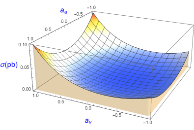
Figure 6: Same as in Fig. 5, but for center-of-mass energy of $\sqrt{s}=10$ $TeV$.

In order to illustrate the contribution of the two interactions, in Figs. 5 and 6 we give the total cross-sections with respect to $\hat{a}_{V}$ and $\hat{a}_{A}$ for center-of-mass energies $\sqrt{s}=7.07\hskip 2.27621ptTeV$ and $10\hskip 2.27621ptTeV$, respectively. As expected, the results are similar in both the cases. In Fig. 6, with an increase in $\sqrt{s}$, the value in the total cross-section rapidly increases and the maximum is achieved either for $\hat{a}_{V}=1$ and $\hat{a}_{A}=1$, or for $\hat{a}_{V}=1$ and $\hat{a}_{A}=-1$. Both figures show great sensitivity with respect to the anomalous couplings $\hat{a}_{V}$ and $\hat{a}_{A}$.

To put our results in perspective with those reported in the literature, we make a direct comparison of our results for the total cross-section as a function of the dipole moments $\hat{a}_{V}$ and $\hat{a}_{A}$ given by Figs. 3 and 4 (or similarly by Figs. 5 and 6), with those reported in Ref. Sh (see Figs. 3 and 4). We find that our results, using the process $e^{-}p\to e^{-}\gamma^{*}\gamma^{*}p\to e^{-}t\bar{t}p$ at the FCC-he energies, show significant improvement as compared to the process $pp\to p\gamma^{*}\gamma^{*}p\to pt\bar{t}p$ at LHC energies. For example, with the process that we have considered in this paper, the total cross-section is a factor ${\cal O}(10^{3})$ between $pp\to p\gamma^{*}\gamma^{*}p\to pt\bar{t}p$ and $e^{-}p\to e^{-}\gamma^{*}\gamma^{*}p\to e^{-}t\bar{t}p$, that is, our results are 3 orders of magnitude higher than those reported in Ref. Sh . This indicates that the sensitivity on the anomalous couplings $\hat{a}_{V}$ and $\hat{a}_{A}$ can be improved at the FCC-he by a few orders of magnitude in comparison with the LHC. In the case of the LHeC, the authors of Ref. Bouzas1 specifically measure $\sigma(\gamma e^{-}\to t\bar{t})$ with $10\%$ $(18\%)$ error, obtaining the following results for the $t$-MM $(\kappa)$ and the $t$-EDM $(\tilde{\kappa})$: $|\kappa|<0.05(0.09)$ and $|\tilde{\kappa}|<0.20(0.28)$. In our case, using the process $e^{-}p\to e^{-}\gamma^{*}\gamma^{*}p\to e^{-}t\bar{t}p$, we obtain: $\hat{a}_{V}=(-0.5014,0.0457)$ and $\hat{a}_{A}=|0.1470|$ with $\delta_{sys}=5\%$, ${\cal L}=1000\hskip 2.27621ptfb^{-1}$ and $95\%\hskip 2.27621ptC.L.$. Although the conditions for the study of both processes $\gamma e^{-}\to t\bar{t}$ and $e^{-}p\to e^{-}\gamma^{*}\gamma^{*}p\to e^{-}t\bar{t}p$ are not the same, our result indicates an improvement of the sensitivity by a factor of 0.914 (0.735) for $\hat{a}_{V}(\hat{a}_{A})$ with respect to the results reported in Ref. Bouzas1 .

III Projections on the dipole moments of the top-quark

We evaluate the potential of top-quark pairs production at the FCC-he with center-of-mass energies of 7.07 and 10 TeV for the measurement of the MM and EDM $\hat{a}_{V}$ and $\hat{a}_{A}$ of the top-quark. To carry out our study, we concentrate on the double top-quark production process, $e^{-}p\to e^{-}\gamma^{*}\gamma^{*}p\to e^{-}t\bar{t}p$, followed by $t(\bar{t})\to bW^{+}(\bar{b}W^{-})$, where the $W$ boson decays into leptons and hadrons.

To probe the sensitivity on the anomalous $\hat{a}_{V}$ and $\hat{a}_{A}$ parameters we perform a $\chi^{2}$ test and calculate $68\%$, $90\%$ and $95\%$ confidence level (C.L.) sensitivities. The $\chi^{2}$ distribution murat ; Billur is defined by:

$$\chi^{2}=\biggl{(}\frac{\sigma_{SM}-\sigma_{BSM}(\sqrt{s},\hat{a}_{V},\hat{a}_{A})}{\sigma_{SM}\sqrt{(\delta_{st})^{2}+(\delta_{sys})^{2}}}\biggr{)}^{2},$$ (27)

with $\sigma_{BSM}(\sqrt{s},\hat{a}_{V},\hat{a}_{A})$ as the total cross-section which contains contributions from the SM and physics BSM, $\delta_{st}=\frac{1}{\sqrt{N_{SM}}}$ and $\delta_{sys}$ are the statistical and systematic uncertainties, respectively. The number of events for the process $e^{-}p\to e^{-}\gamma^{*}\gamma^{*}p\to e^{-}t\bar{t}p$ is given by $N_{SM}={\cal L}_{int}\times\sigma_{SM}\times BR\times\epsilon_{b-tag}\times\epsilon_{b-tag}$, where ${\cal L}_{int}$ is the integrated luminosity and $b$-jet tagging efficiency is $\epsilon_{b}=0.8$ atlas . The top-quark decay almost $100\%$ into a $W$ boson and a $b$ quark. For top-quark pair production, we can categorize decay products according to the decomposition of $W$. In this work, we assume that for the signal, one of the $W$ bosons decays leptonically and the other hadronically. This event has already been studied by ATLAS and CMS Collaborations cmstop1 ; cmstop2 ; atlastop . It is worth mentioning that the branching rations for $W$ decay are: $BR(W\to qq^{\prime})=0.674$ for hadronic decay, $BR(W\to l\nu_{e,\mu})=0.213$ for light leptonic decays and $BR(W\to\tau\nu_{\tau})=0.113$ Data2018 . Therefore, for $t\bar{t}$ production followed by $t\to Wb$ decays, the branching rations for the dominant channels are the hadronic and semileptonic, respectively. Thus, we assume that the branching ratio of the top-quark pair in the final state is $BR(t\to Wb)=0.286$.

An important part of our study is the incorporation of theoretical uncertainties as there may be several experimental and systematic uncertainty sources in top-quark identification. In hadron colliders, especially the LHC, the process of determining the cross-section of top pair production has been experimentally studied topuncertanintyatlas ; topuncertaintycms . From these studies, the total systematic uncertainty value is about 10$\%$ and is increasingly improved when it is compared with previous experimental studies cmstop2 .

Tables II-VII show the projections for model-independent sensitivity on the dipole moments $\hat{a}_{V}$ and $\hat{a}_{A}$ of the top-quark at the FCC-he. We assume center-of-mass energies of $7.07\hskip 2.27621ptTeV$ and $10\hskip 2.27621ptTeV$, integrated luminosity ${\cal L}=50,100,300,500,1000\hskip 2.27621ptfb^{-1}$, systematic uncertainties $\delta_{sys}=0\%,3\%,5\%$, and we determine $68\%$, $90\%$ and $95\%$ C.L. sensitivities. We find that the mode of top-quark pair production $e^{-}p\to e^{-}\gamma^{*}\gamma^{*}p\to e^{-}t\bar{t}p$ imposes stronger sensitivities on the dipole moments. In conclusion, the FCC-he can measure the electromagnetic dipole moments of the top-quark with a sensitivity of the order ${\cal O}(10^{-2}-10^{-1})$ at $95\%\hskip 2.27621ptC.L.$.

It is worthwhile to compare the results obtained here with those of Ref. Sh which consider the process $pp\to p\gamma^{*}\gamma^{*}p\to pt\bar{t}p$ with the LHC running at $\sqrt{s}=14,33\hskip 2.27621ptTeV$ and with integrated luminosities of ${\cal L}=100,300,3000\hskip 2.27621ptfb^{-1}$. The authors of Ref. Sh find constraints at $68\%\hskip 2.27621ptC.L.$ of the order ${\cal O}(10^{-2}-10^{-1})$. We also note that, while we do consider three systematic errors in our study, the quoted sensitivities in Ref. Sh do not include theoretical uncertainty. Furthermore, the FCC-he sensitivity is even higher in our process than in that reported in Ref. Sh .

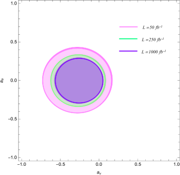
Figure 7: Sensitivity contours at the $95\%\hskip 2.84526ptC.L.$ in the $\hat{a}_{V}-\hat{a}_{A}$ plane through the process $e^{-}p\to e^{-}\gamma^{*}\gamma^{*}p\to e^{-}t\bar{t}p$ for $\sqrt{s}=7.07$ $TeV$ at the FCC-he.

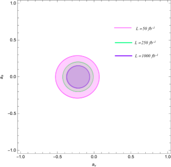
Figure 8: Same as in Fig. 7, but for $\sqrt{s}=10$ $TeV$.

Figs. 7 and 8 show the sensitivity contours at the $95\%\hskip 2.84526ptC.L.$ in the $\hat{a}_{V}-\hat{a}_{A}$ plane through the process $e^{-}p\to e^{-}\gamma^{*}\gamma^{*}p\to e^{-}t\bar{t}p$ for $\sqrt{s}=7.07\hskip 2.27621ptTeV,10\hskip 2.27621ptTeV$ and ${\cal L}=50,250,1000\hskip 2.27621ptfb^{-1}$ at the FCC-he. We find that the sensitivity of the anomalous couplings can be increased with an increase in the luminosity as the couplings scales as $1/\sqrt{\cal L}$ for a given $\chi^{2}$. Thus for $1000fb^{-1}$, the sensitivity of $\hat{a}_{V}$ and $\hat{a}_{A}$ is improved with respect to $50fb^{-1}$ and $250fb^{-1}$, respectively. Concentrating on the sensitivity at $95\%$ C.L., we observe that only contributions to the dipole moments at the order $\hat{a}_{V}=(-0.5900,0.1188)$ and $\hat{a}_{A}=|0.2567|$ could be detected with $50\hskip 2.27621ptfb^{-1}$. With higher luminosity, these sensitivities improve up to $\hat{a}_{V}=(-0.4864,0.0332)$ and $\hat{a}_{A}=|0.1233|$ (at $1000\hskip 2.27621ptfb^{-1}$) (see Table VII). Compared with the sensitivities of Table I, which arise in different contexts, a significant improvement can be obtained.

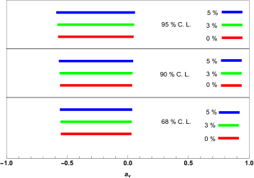
Figure 9: The expected sensitivities of FCC-he measurements at $\sqrt{s}=7.07\hskip 2.27621ptTeV$ to $\hat{a}_{V}$ in the process $e^{-}p\to e^{-}\gamma^{*}\gamma^{*}p\to e^{-}t\bar{t}p$. We assume systematic uncertainties $\delta_{sys}=0,3,5\hskip 2.27621pt\%$ and $68\%,90\%,95\%\hskip 2.27621ptC.L.$.

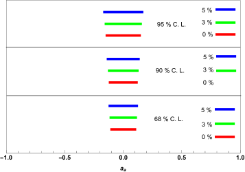
Figure 10: Same as in Fig. 9, but for $\hat{a}_{A}$.

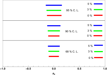
Figure 12: Same as in Fig. 11, but for $\hat{a}_{A}$.

We use channel $e^{-}p\to e^{-}\gamma^{*}\gamma^{*}p\to e^{-}t\bar{t}p$ to make fits to estimate the sensitivities at the various FCC-he center-of-mass energies, using the dependence of the total cross-section on the parameters $\hat{a}_{V}$ and $\hat{a}_{A}$, as shown by Eqs. (23)-(26). In making our $\chi^{2}$ fits, we adopt statistical errors $\delta_{st}=\frac{1}{\sqrt{N_{SM}}}$ (see Eq. (27) ), and we assume systematic uncertainties $\delta_{sys}=0,3\%,5\%$. The sensibility results at $68\%$, $90\%$ and $95\%$ C.L. are plotted in Figs. 9-12 for $7.07\hskip 2.27621ptTeV$ and $10\hskip 2.27621ptTeV$, respectively.

The results from our $7.07\hskip 2.27621ptTeV$ fit shown in Figs. 9 and 10 include the individual sensitivity obtained considering just one parameter at a time and the estimated sensitivities are color-coded in red, green and blue. In these figures, the sensitivities are obtained by taking into account the systematic uncertainties $\delta_{sys}=0\%,3\%,5\%$ at $68\%$, $90\%$ and $95\%$ C.L., respectively.

Similar conclusions hold for the $10\hskip 2.27621ptTeV$ fits whose results are shown in Figs. 11 and 12, where the increases in sensitivity are even more notable with individual sensitivities on $\hat{a}_{V}$ and $\hat{a}_{A}$. This level of sensitivity becomes comparable to that at which future electroweak precision tests may constrain the anomalous couplings $\hat{a}_{V}$ and $\hat{a}_{A}$ as is the case of the ILC and CLIC Aguilar ; murat ; Billur .

IV Conclusions

In this paper, we have emphasized the potential importance for sensitivity of the FCC-he, that is, of a future high-energy $e^{-}p$ collider for directly probing possible new physics BSM by studying sensitivity on the total cross-section and on the $\hat{a}_{V}$ and $\hat{a}_{A}$ at $\sqrt{s}=7.07,10\hskip 2.27621ptTeV$ and ${\cal L}=50$ to $1000\hskip 2.27621ptfb^{-1}$. We have stressed and shown numerically (see Figs. 3-12 and Tables II-VII), that the increase sensitivity at high energy and high luminosity provides opportunities in the process $e^{-}p\to e^{-}\gamma^{*}\gamma^{*}p\to e^{-}t\bar{t}p$ in particular. The extracted results for the FCC-he, presented in Figs 3-12 and Tables II-VII, show very high sensitivity, and in some cases improvements are expected with respect to the potential sensitivity for the LHC, ILC and CLIC (see Table I and Refs. Ibrahim ; Atwood ; Polouse ; Choi ; Polouse1 ; Aguilar0 ; Amjad ; Juste ; Asner ; Abe ; Aarons ; Brau ; Baer ; Grzadkowski:2005ye ). Our results motivate more detailed studies including additional benchmark analyses based on full FCC-he detector simulations at high energies with the aim of verifying and refining our estimates on the sensitivity with which the cross-sections and the $t$-MM and $t$-EDM for the process $e^{-}p\to e^{-}\gamma^{*}\gamma^{*}p\to e^{-}t\bar{t}p$ could be measured at the FCC-he. It is worth mentioning that, in comparison with the LHC, the FCC-he has the advantage of providing a clean environment with small background contributions from QCD strong interactions. With all these arguments already presented, we conclude that the FCC-he is a viable option for model-independent sensitivity estimates on top-quark anomalous electromagnetic couplings with very good accuracy.

Table 2: Sensitivity on the $\hat{a}_{V}$ magnetic moment and the $\hat{a}_{A}$ electric dipole moment for the process $e^{-}p\to e^{-}\gamma^{*}\gamma^{*}p\to e^{-}t\bar{t}p$ for $\sqrt{s}=7.07\hskip 2.27621ptTeV$ and ${\cal L}=50,100,300,500,1000\hskip 2.27621ptfb^{-1}$ at $68\%$ C.L..

$\sqrt{s}=7.07\hskip 2.27621ptTeV$,           $68\%$ C.L.
${\cal L}\hskip 2.27621pt(fb^{-1})$	$\delta_{sys}$	$\hat{a}_{V}$	$\hskip 48.36958pt|\hat{a}_{A}|$
50	$0\%$	[-0.6190, 0.0791]	0.2107
50	$3\%$	[-0.6196, 0.0796]	0.2114
50	$5\%$	[-0.6206, 0.0804]	0.2127
100	$0\%$	[-0.5918, 0.0588]	0.1777
100	$3\%$	[-0.5927, 0.0595]	0.1789
100	$5\%$	[-0.5943, 0.0607]	0.1810
300	$0\%$	[-0.5616, 0.0359]	0.1355
300	$3\%$	[-0.5634, 0.0372]	0.1381
300	$5\%$	[-0.5663, 0.0394]	0.1425
500	$0\%$	[-0.5518, 0.0284]	0.1193
500	$3\%$	[-0.5540, 0.0301]	0.1232
500	$5\%$	[-0.5577, 0.0329]	0.1293
1000	$0\%$	[-0.5415, 0.0204]	0.1005
1000	$3\%$	[-0.5447, 0.0229]	0.1067
1000	$5\%$	[-0.5496, 0.0267]	0.1156

Table 3: Sensitivity on the $\hat{a}_{V}$ magnetic moment and the $\hat{a}_{A}$ electric dipole moment for the process $e^{-}p\to e^{-}\gamma^{*}\gamma^{*}p\to e^{-}t\bar{t}p$ for $\sqrt{s}=7.07\hskip 2.27621ptTeV$ and ${\cal L}=50,100,300,500,1000\hskip 2.27621ptfb^{-1}$ at $90\%$ C.L..

$\sqrt{s}=7.07\hskip 2.27621ptTeV$,           $90\%$ C.L.
${\cal L}\hskip 2.27621pt(fb^{-1})$	$\delta_{sys}$	$\hat{a}_{V}$	$\hskip 48.36958pt|\hat{a}_{A}|$
50	$0\%$	[-0.6434, 0.0972]	0.2107
50	$3\%$	[-0.6441, 0.0978]	0.2114
50	$5\%$	[-0.6454, 0.0987]	0.2127
100	$0\%$	[-0.6106, 0.0729]	0.2009
100	$3\%$	[-0.6117, 0.0737]	0.2022
100	$5\%$	[-0.6137, 0.0752]	0.2045
300	$0\%$	[-0.5736, 0.0451]	0.1533
300	$3\%$	[-0.5758, 0.0467]	0.1563
300	$5\%$	[-0.5793, 0.0494]	0.1612
500	$0\%$	[-0.5614, 0.0357]	0.1351
500	$3\%$	[-0.5642, 0.0379]	0.1394
500	$5\%$	[-0.5688, 0.0413]	0.1463
1000	$0\%$	[-0.5485, 0.0259]	0.1137
1000	$3\%$	[-0.5526, 0.0290]	0.1207
1000	$5\%$	[-0.5587, 0.0336]	0.1308

Table 4: Sensitivity on the $\hat{a}_{V}$ magnetic moment and the $\hat{a}_{A}$ electric dipole moment for the process $e^{-}p\to e^{-}\gamma^{*}\gamma^{*}p\to e^{-}t\bar{t}p$ for $\sqrt{s}=7.07\hskip 2.27621ptTeV$ and ${\cal L}=50,100,300,500,1000\hskip 2.27621ptfb^{-1}$ at $95\%$ C.L..

$\sqrt{s}=7.07\hskip 2.27621ptTeV$,           $95\%$ C.L.
${\cal L}\hskip 2.27621pt(fb^{-1})$	$\delta_{sys}$	$\hat{a}_{V}$	$\hskip 48.36958pt|\hat{a}_{A}|$
50	$0\%$	[-0.6959, 0.1357]	0.2922
50	$3\%$	[-0.6969, 0.1364]	0.2931
50	$5\%$	[-0.6986, 0.1377]	0.2948
100	$0\%$	[-0.6518, 0.1035]	0.2471
100	$3\%$	[-0.6534, 0.1046]	0.2487
100	$5\%$	[-0.6560, 0.1065]	0.2515
300	$0\%$	[-0.6007, 0.0654]	0.1889
300	$3\%$	[-0.6037, 0.0677]	0.1926
300	$5\%$	[-0.6087, 0.0714]	0.1986
500	$0\%$	[-0.5833, 0.0523]	0.1665
500	$3\%$	[-0.5873, 0.0554]	0.1719
500	$5\%$	[-0.5938, 0.0603]	0.1803
1000	$0\%$	[-0.5648, 0.0383]	0.1403
1000	$3\%$	[-0.5706, 0.0427]	0.1489
1000	$5\%$	[-0.5794, 0.0494]	0.1613

Table 5: Sensitivity on the $\hat{a}_{V}$ magnetic moment and the $\hat{a}_{A}$ electric dipole moment for the process $e^{-}p\to e^{-}\gamma^{*}\gamma^{*}p\to e^{-}t\bar{t}p$ for $\sqrt{s}=10\hskip 2.27621ptTeV$ and ${\cal L}=50,100,300,500,1000\hskip 2.27621ptfb^{-1}$ at $68\%$ C.L..

$\sqrt{s}=10\hskip 2.27621ptTeV$,           $68\%$ C.L.
${\cal L}\hskip 2.27621pt(fb^{-1})$	$\delta_{sys}$	$\hat{a}_{V}$	$\hskip 48.36958pt|\hat{a}_{A}|$
50	$0\%$	[-0.5292, 0.0689]	0.1852
50	$3\%$	[-0.5298, 0.0694]	0.1860
50	$5\%$	[-0.5310, 0.0703]	0.1875
100	$0\%$	[-0.5077, 0.0511]	0.1562
100	$3\%$	[-0.5087, 0.0519]	0.1576
100	$5\%$	[-0.5104, 0.0533]	0.1601
300	$0\%$	[-0.4839, 0.0311]	0.1191
300	$3\%$	[-0.4857, 0.0327]	0.1222
300	$5\%$	[-0.4888, 0.0352]	0.1273
500	$0\%$	[-0.4761, 0.0245]	0.1049
500	$3\%$	[-0.4785, 0.0266]	0.1094
500	$5\%$	[-0.4823, 0.0298]	0.1163
1000	$0\%$	[-0.4680, 0.0177]	0.0883
1000	$3\%$	[-0.4714, 0.0205]	0.0955
1000	$5\%$	[-0.4763, 0.0247]	0.1053

Table 6: Sensitivity on the $\hat{a}_{V}$ magnetic moment and the $\hat{a}_{A}$ electric dipole moment for the process $e^{-}p\to e^{-}\gamma^{*}\gamma^{*}p\to e^{-}t\bar{t}p$ for $\sqrt{s}=10\hskip 2.27621ptTeV$ and ${\cal L}=50,100,300,500,1000\hskip 2.27621ptfb^{-1}$ at $90\%$ C.L..

$\sqrt{s}=10\hskip 2.27621ptTeV$,           $90\%$ C.L.
${\cal L}\hskip 2.27621pt(fb^{-1})$	$\delta_{sys}$	$\hat{a}_{V}$	$\hskip 48.36958pt|\hat{a}_{A}|$
50	$0\%$	[-0.5485, 0.0848]	0.2092
50	$3\%$	[-0.5492, 0.0854]	0.2101
50	$5\%$	[-0.5506, 0.0865]	0.2117
100	$0\%$	[-0.5226, 0.0634]	0.1766
100	$3\%$	[-0.5238, 0.0644]	0.1782
100	$5\%$	[-0.5259, 0.0661]	0.1809
300	$0\%$	[-0.4934, 0.0391]	0.1347
300	$3\%$	[-0.4957, 0.0410]	0.1383
300	$5\%$	[-0.4994, 0.0441]	0.1440
500	$0\%$	[-0.4837, 0.0309]	0.1187
500	$3\%$	[-0.4867, 0.0334]	0.1238
500	$5\%$	[-0.4914, 0.0374]	0.1316
1000	$0\%$	[-0.4735, 0.0224]	0.1000
1000	$3\%$	[-0.4778, 0.0260]	0.1081
1000	$5\%$	[-0.4840, 0.0311]	0.1192

Table 7: Sensitivity on the $\hat{a}_{V}$ magnetic moment and the $\hat{a}_{A}$ electric dipole moment for the process $e^{-}p\to e^{-}\gamma^{*}\gamma^{*}p\to e^{-}t\bar{t}p$ for $\sqrt{s}=10\hskip 2.27621ptTeV$ and ${\cal L}=50,100,300,500,1000\hskip 2.27621ptfb^{-1}$ at $95\%$ C.L..

$\sqrt{s}=10\hskip 2.27621ptTeV$,           $95\%$ C.L.
${\cal L}\hskip 2.27621pt(fb^{-1})$	$\delta_{sys}$	$\hat{a}_{V}$	$\hskip 48.36958pt|\hat{a}_{A}|$
50	$0\%$	[-0.5900, 0.1188]	0.2567
50	$3\%$	[-0.5910, 0.1196]	0.2578
50	$5\%$	[-0.5928, 0.1211]	0.2598
100	$0\%$	[-0.5551, 0.0903]	0.2171
100	$3\%$	[-0.5568, 0.0916]	0.2191
100	$5\%$	[-0.5596, 0.0939]	0.2224
300	$0\%$	[-0.5147, 0.0569]	0.1660
300	$3\%$	[-0.5179, 0.0595]	0.1704
300	$5\%$	[-0.5232, 0.0639]	0.1774
500	$0\%$	[-0.5010, 0.0454]	0.1464
500	$3\%$	[-0.5053, 0.0490]	0.1527
500	$5\%$	[-0.5120, 0.0546]	0.1622
1000	$0\%$	[-0.4864, 0.0332]	0.1233
1000	$3\%$	[-0.4925, 0.0383]	0.1334
1000	$5\%$	[-0.5014, 0.0457]	0.1470

Acknowledgments

A. G. R. and M. A. H. R. acknowledge support from SNI and PROFOCIE (México).

Figure 3: The total cross sections of the process $e^{-}p\to e^{-}\gamma^{*}\gamma^{*}p\to e^{-}t\bar{t}p$ as a function of $\hat{a}_{V}$ for center-of-mass energies of $\sqrt{s}=7.07,10$ $TeV$ at the FCC-he.

Figure 11: Same as in Fig. 9, but for $\sqrt{s}=10\hskip 2.27621ptTeV$.

References

• (1) M. Tanabashi, et al., [Particle Data Group], Phys. Rev. D 98, 030001 (2018).
• (2) F. Englert and R. Brout, Phys. Rev. Lett. 13, 321 (1964).
• (3) P. W. Higgs, Phys. Lett. 12, 132 (1964).
• (4) P. W. Higgs, Phys. Rev. Lett. 13, 508 (1964).
• (5) G. S. Guralnik, C. R. Hagen and T. W. B. Kibble, Phys. Rev. Lett. 13, 585 (1964).
• (6) G. Aad, et al., [ATLAS Collaboration], Phys. Lett. B716, 1 (2012).
• (7) S. Chatrchyan, et al., [CMS Collaboration], Phys. Lett. B716, 30 (2012).
• (8) Oliver Brüning, John Jowett, Max Klein, Dario Pellegrini, Daniel Schulte and Frank Zimmermann, EDMS 17979910 FCC-ACC-RPT-0012, V1.0, 6 April, 2017. https://fcc.web.cern.ch/Documents/FCCheBaselineParameters.pdf.
• (9) J. L. A. Fernandez, et al.. [LHeC Study Group], J. Phys. G39, 075001 (2012).
• (10) J. L. A. Fernandez, et al., [LHeC Study Group], arXiv:1211.5102.
• (11) J. L. A. Fernandez, et al., arXiv:1211.4831.
• (12) Huan-Yu, Bi, Ren-You Zhang, Xing-Gang Wu, Wen-Gan Ma, Xiao-Zhou Li and Samuel Owusu, Phys. Rev. D95, 074020 (2017).
• (13) Y. C. Acar, A. N. Akay, S. Beser, H. Karadeniz, U. Kaya, B. B. Oner, S. Sultansoy, Nuclear Inst. and Methods in Physics Research A871, 47 (2017).
• (14) O. Bruening and M. Klein, Mod. Phys. Lett. A28, 1330011 (2013).
• (15) W. Bernreuther, R. Bonciani, T. Gehrmann, R. Heinesch, T. Leineweber, P. Mastrolia, E. Remiddi, Phys. Rev. Lett. 95, 261802 (2005).
• (16) F. Hoogeveen, Nucl. Phys. B341, 322 (1990).
• (17) M. E. Pospelov and I. B. Khriplovich, Sov. J. Nucl. Phys. 53, 638 (1991) [Yad. Fiz. 53 (1991) 1030].
• (18) A. Soni and R. M. Xu, Phys. Rev. Lett. 69, 33 (1992).
• (19) Juste A., Kiyo Y., Petriello F., Teubner T., Agashe K., Batra P., Baur U., Berger C. F., et al., hep-ph/0601112.
• (20) U. Baur, A. Juste, L. H. Orr and D. Rainwater, Phys. Rev. D71, 054013 (2005).
• (21) A. O. Bouzas and F. Larios, Phys. Rev. D87, 074015 (2013).
• (22) Sh. Fayazbakhsh, S. Taheri Monfared and M. Mohammadi Najafabadi, Phys. Rev. D92, 014006 (2015).
• (23) A. O. Bouzas and F. Larios, Phys. Rev. D88, 094007 (2013).
• (24) Aguilar-Saavedra J. A., et al., [ECFA/DESY LC Physics Working Group Collaboration], hep-ph/0106315.
• (25) M. Köksal, A. A. Billur and A. Gutiérrez-Rodríguez, Adv. High Energy Phys. 2017, 6738409 (2017).
• (26) A. A. Billur, M. Köksal and A. Gutiérrez-Rodríguez, Phys. Rev. D96, 056007 (2017).
• (27) T. Ibrahim and P. Nath, Phys. Rev. D82, 055001 (2010).
• (28) D. Atwood, A. Aeppli and A. Soni, Phys. Rev. Lett. 69, 2754 (1992).
• (29) P. Poulose and S. D. Rindani, Phys. Rev. D57, 5444 (1998) [Erratum-ibid. D61 , 119902 (2000)].
• (30) S. Y. Choi and K. Hagiwara, Phys. Lett. B359, 369 (1995).
• (31) P. Poulose and S. D. Rindani, Phys. Rev. D91, 093008 (2015).
• (32) J. A. Aguilar-Saavedra, et al., [TESLA: The Superconducting electron positron linear collider with an integrated x-ray laser laboratory. Technical design report. Part 3. Physics at an $e^{+}e^{-}$ linear collider], arXiv:hep-ph/0106315.
• (33) M. Amjad, M. Boronat, T. Frisson, I. G. García, R. P$\ddot{o}$schl, et al., arXiv:1307.8102 [hep-ex].
• (34) D. Asner, et al., arXiv:1307.8265 [hep-ex].
• (35) T. Abe, et al., [American Linear Collider Working Group Collaboration], arXiv:hep-ex/0106057.
• (36) G. Aarons, et al., [ILC Collaboration], arXiv:0709.1893 [hep-ph].
• (37) J. Brau, et al., [ILC Collaboration], arXiv:0712.1950 [physics.acc-ph].
• (38) H. Baer, T. Barklow, K. Fujii, et al., arXiv:1306.6352 [hep-ph].
• (39) B. Grzadkowski, Z. Hioki, K. Ohkuma and J. Wudka, JHEP 0511, 029 (2005).
• (40) J. F. Kamenik, M. Papucci and A. Weiler, Phys. Rev. D85, 071501 (2012).
• (41) J. A. Aguilar-Saavedra, M. C. N. Fiolhais and A. Onofre, JHEP 07, 180 (2012).
• (42) W. Buhmuller and D. Wyler, Nul. Phys. B268, 621 (1986).
• (43) J. A. Aguilar-Saavedra, Nucl. Phys. B812, 181 (2009).
• (44) V. M. Budnev, I. F. Ginzburg, G. V. Meledin and V. G. Serbo, Phys. Rep. 15, 181 (1975).
• (45) G. Baur, et al., Phys. Rep. 364, 359 (2002).
• (46) K. Piotrzkowski, Phys. Rev. D63, 071502 (2001).
• (47) A. Abulencia, et al., [CDF Collaboration], Phys. Rev. Lett. 98, 112001 (2007).
• (48) T. Aaltonen, et al., [CDF Collaboration], Phys. Rev. Lett. 102, 222002 (2009).
• (49) T. Aaltonen, et al., [CDF Collaboration], Phys. Rev. Lett. 102, 242001 (2009).
• (50) S. Chatrchyan, et al., [CMS Collaboration], JHEP 1201, 052 (2012).
• (51) S. Chatrchyan, et al., [CMS Collaboration], JHEP 1211, 080 (2012).
• (52) V. M. Abazov, et al., [D0 Collaboration], Phys. Rev. D88, 012005 (2013).
• (53) S. Chatrchyan, et al., [CMS Collaboration], JHEP 07, 116 (2013).
• (54) A. Belyaev, N. D. Christensen and A. Pukhov, Comput. Phys. Commun. 184, 1729 (2013).
• (55) ATLAS Collaboration, Report No. ATL-PHYS-PUB-2015-39.
• (56) ATLAS Collaboration, Eur. Phys. J. C71, 1577 (2011).
• (57) CMS Collaboration, Phys. Lett. B695, 424 (2011).
• (58) CMS Collaboration, Eur. Phys. J. C71, 1721 (2011).
• (59) M. Tanabashi, et al., [Particle Data Group], Phys. Rev. D98, 030001 (2018).
• (60) ATLAS Collaboration, Phys. Lett. B761, 136 (2016).
• (61) V. Khachatryan, et al. [CMS Collaboration], Phys. Rev. Lett. 116, 052002 (2016).
Refer to caption