Abundant Serendipitous Emission Line Sources with JWST/NIRSpec

Abstract

The James Webb Space Telescope will provide observational capabilities that far exceed those of current ground- or space-based instrumentation. In particular, the NIRSpec instrument will take highly sensitive spectroscopic data for hundreds of objects simultaneously from 0.6$-$5.3 $\mu$m. Current photometric observations suggest a large and increasing number of faint ($M_{\mathrm{UV}}$ $>-$16) galaxies at high-redshift, with increasing evidence that galaxies at these redshifts have optical emission lines with extremely high equivalent widths. A simple model of their emission line fluxes and number density evolution with redshift is used to predict the number of galaxies that NIRSpec will serendipitously observe during normal observations with the microshutter array. At exposure times of $\approx$ 20 hours in the low-resolution prism mode, the model predicts that, on average, every open 1$\times$3 ‘microslit’ will contain an un-targeted galaxy with a detectable [O iii] and/or H $\alpha$ emission line; while most of these detections are predicted to be of [O iii], H $\alpha$ detections alone would still number 0.56 per open ‘microslit’ for this exposure time. Many of these objects are spectroscopically detectable even when they are fainter than current photometric limits and/or their flux centroids lie outside of the open microshutter area. The predicted number counts for such galaxies match $z\sim 2$ observations of [O iii] emitters from slitless grism spectroscopic surveys, as well as theoretical predictions based on sophisticated modeling of galaxy spectral energy distributions. These serendipitous detections could provide the largest numbers of $z>6$ spectroscopic confirmations in the deepest NIRSpec surveys.

1 INTRODUCTION

The James Webb Space Telescope (JWST; Gardner et al., 2006) represents the most significant new space-based observatory at optical and near-infrared wavelengths of the current decade. Currently scheduled to launch by March 2021, JWST’s spectroscopic capabilities from 0.6 to 28.8 $\mu$m far exceed those of existing observatories, such as the Hubble Space Telescope (HST) or the Spitzer Space Telescope. In particular, the Near-Infrared Spectrograph (NIRSpec; Bagnasco et al., 2007; Birkmann et al., 2010) will give us unprecedented spectral sensitivity and multi-object capabilities (in the multi-object spectroscopy or ‘MOS’ mode) with uninterrupted coverage from 0.6$-$5.3 $\mu$m.

This red wavelength coverage is required to detect bright restframe-optical emission lines, such as H $\alpha$ and [O iii] $\lambda$5007, at high-$z$ since current ground-based observations are typically limited to the $K$-band which extends out to $\sim$2.4 $\mu$m and hence $z\lesssim 4$. JWST/NIRSpec will detect these lines out to $z\sim 9.6$ with one to two orders of magnitude higher spectroscopic sensitivity than existing instruments. With the configurable microshutter array (MSA), NIRSpec can deliver up to $\sim$200 non-overlapping spectra simultaneously. This will be crucial in obtaining spectroscopic confirmations of the numerous high-$z$ galaxy candidates that have so far been detected primarily through HST imaging (e.g. Stanway et al., 2003; Bunker et al., 2004; Dickinson et al., 2004; Bouwens et al., 2017; Livermore et al., 2017; Atek et al., 2018; Ishigaki et al., 2018).

Recent observations have pointed to an abundant population of faint ($M_{\mathrm{UV}}$ $>$ $-$18) $z\gtrsim 4$ galaxies that are often difficult to study spectroscopically due to the intrinsic faintness of the UV (metal) emission lines and the absorption of the powerful Ly $\alpha$ line from the neutral intergalactic medium for galaxies in the reionization epoch (Vanzella et al., 2014). However, photometric techniques have been developed to study the restframe-optical emission line properties of these galaxies: the existence of bright, high-equivalent width (EW) optical emission lines in $z\gtrsim 4$ galaxies is inferred by measuring strong excesses in broad-band Spitzer/IRAC 3.6 $\mu$m and/or 4.5 $\mu$m photometry (e.g. Shim et al., 2011; González et al., 2012; Labbé et al., 2013; Stark et al., 2013; Smit et al., 2014). With EWs of [O iii] and H $\alpha$ often in excess of 500 Å (restframe), these lines should be readily detectable with moderately-deep NIRSpec observations.

Obtaining large spectroscopic samples of $z\gtrsim 4$ galaxies is one of the primary goals of NIRSpec. These samples will be crucial in understanding galaxy formation and evolution, from the contribution of galaxies to the reionization of the universe (e.g. Bouwens et al., 2012; Finkelstein et al., 2012; Robertson et al., 2013) and the relationship between galaxies and accreting supermassive black holes (e.g. Vito et al., 2018), to the build-up of the stellar mass of the universe (e.g. Duncan et al., 2014) and the chemical enrichment histories of the star-forming population (e.g. Maiolino et al., 2008). Even when we have access to exquisite JWST/NIRCam imaging, precise spectroscopic redshifts will be necessary to fully interpret a galaxy’s spectral energy distribution (SED; e.g. Wilkins et al., 2013). If ‘serendipitous’ sources that are not the primary target of observations contribute to the number counts of a NIRSpec survey, then NIRSpec becomes an even more powerful tool to assemble these large samples.

Using integral field unit (IFU) spectroscopy, Brinchmann et al. (2017) show that faint galaxies often have (spectroscopically-detectable) ‘contaminants’ located nearby in projection: between 5 and 10 per cent of galaxies with $F775W$ magnitudes between 25 and 26 have a projected companion within 0$\aas@@fstack{\prime\prime}$5 that has a brighter emission line than the strongest line in the primary galaxy. While this was discussed in the context of contamination in photometric versus spectroscopic redshift surveys, Brinchmann et al. (2017) find that spectroscopic observations with a spatial resolution of 0$\aas@@fstack{\prime\prime}$5 will be contaminated by an object with stronger emission lines 1 per cent of the time. Even though high-$z$ sources are expected to be small in size ($r_{e}\sim 0\aas@@fstack{\prime\prime}1$ at $z=6$; Shibuya et al., 2015; Curtis-Lake et al., 2016), the large and under-sampled NIRSpec point spread function (PSF), particularly at wavelengths $>$ 3 $\mu$m, also means that flux from these objects will be dispersed onto the detector even if they lie outside the 0$\aas@@fstack{\prime\prime}$20 $\times$ 0$\aas@@fstack{\prime\prime}$46 open area of each microshutter. In addition, many of these sources could have spectroscopically-detectable emission lines even with continuum magnitudes below imaging detection limits (cf. Ellis et al., 2001; Rauch et al., 2008; Cassata et al., 2011; Henry et al., 2012; Bacon et al., 2017; Maseda et al., 2018b), making their characterisation with NIRSpec even more crucial.

Given the sensitivity of NIRSpec, the size of the open area of each microshutter, and the number of simultaneous spectra that can be obtained (up to 200 per configuration), we would therefore expect a significant number of ‘contaminating’ spectra in a NIRSpec observation, even more so when coupled with the aforementioned evolution in the highest-EW optical emission lines with redshift. This also extends beyond the estimation of the number of contaminants with stronger emission lines: the primary concern is the number of spectroscopically-detectable emission line sources, agnostic as to whether they are brighter than the primary spectroscopic target.

To this end, we develop a model, based on continuum UV luminosity functions (Section 2), for the evolution of emission line fluxes (H $\alpha$ and [O iii]) with redshift (Section 3). With a realistic model for NIRSpec multi-object observations (Section 4), we estimate the number of ‘serendipitous emission line sources’ that are detectable as a function of observing mode and observing time (Section 5). Caveats and the interpretation of the results from the model are also presented (Section 6). ‘Microshutter’ refers to a single 0$\aas@@fstack{\prime\prime}$20 $\times$ 0$\aas@@fstack{\prime\prime}$46 MSA shutter while ‘microslit’ refers to a 1$\times$3 configuration of open microshutters (1$\aas@@fstack{\prime\prime}$52 tall, including the bars between shutters). We adopt a flat $\Lambda$CDM cosmology ($\Omega_{m}=0.3$, $\Omega_{\Lambda}=0.7$, and H${}_{0}=70~{}$km s^-1 Mpc^-1) and AB magnitudes (Oke, 1974) throughout.

2 UV Luminosity Functions

Galaxy luminosity functions are traditionally fit with a Schechter function (Schechter, 1976) of the form:

$$n(M)\ \mathrm{d}M=0.4\ \ln 10\ \phi^{\star}[10^{0.4(M^{\star}-M)}]^{\alpha+1}e^{[-10^{0.4(M^{\star}-M)}]}\ \mathrm{d}M,$$ (1)

describing the number of galaxies $n$ of a given magnitude $M$, where $\phi^{\star}$ is the normalisation (units of Mpc^-3), $M^{\star}$ is the characteristic magnitude, and $\alpha$ is the faint-end power law slope. An equivalent form of this function can be written in terms of luminosity $L$ instead of $M$.

Predictions for the volume density of galaxies with a given $M_{\mathrm{UV}}$ have been made from the local universe out to the highest observed redshifts. Here, we combine results from many studies to determine a single UV luminosity function parametrized by redshift (see also Parsa et al., 2016; Williams et al., 2018). We fit linear functions to the Schechter function parameters $\alpha$(z) and log₁₀ $\phi_{\star}$(z), and a fourth-order polynomial to $M_{\star,\mathrm{UV}}$($z$) to reproduce the asymptotic behavior at high-$z$ (Bouwens et al., 2015); see Figure 1. These parameters are listed in Table 2. The $M_{\star,\mathrm{UV}}$ values from the literature span a range in restframe wavelength from 1500 to 1700 Å which we consider to be $M_{\star,1550}$ as the average galaxy in these samples has a negligible $K$-correction from these wavelengths to 1550 Å (Oesch et al., 2009). The best-fit parameterizations are:

$$\alpha(z)=-0.131\times z-1.14,$$ (2)

$$log_{10}~{}\phi_{\star}(z)=-0.228\times z-2.10,$$ (3)

and

$$M_{\star}(z)=-0.0112\times z^{3}+0.241\times z^{2}-1.55\times z-17.8.$$ (4)

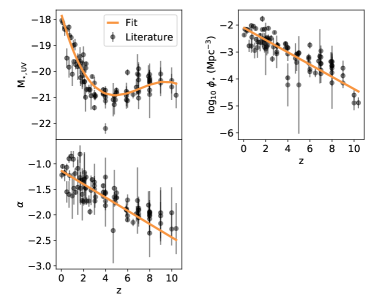
Figure 1: Literature data (Table 2) and polynomial fits to $\alpha$, M_⋆,UV, and log${}_{10}~{}\phi_{\star}$ as a function of redshift. For M_⋆,UV, the fit is a third-order polynomial to capture the flattening of the relation at high-z (Bouwens et al., 2015) and is measured at $\sim$1550 Å. The results of the fits are given in Equations 2, 3, and 4.

The faint-end slope of the galaxy UV luminosity function has recently received considerable attention. In particular, at $z\sim 6$ many authors have used data from the Hubble Frontier Fields (Lotz et al., 2017), leveraging gravitational lensing to find extremely faint galaxies. As mentioned before, the interest in the number density of such faint galaxies is due to the potential contribution of such faint ($M_{\mathrm{UV}}$ $>-$16) galaxies to cosmic reionization. However, the numbers of photometric candidates at these faint limits are small and large uncertainties on the lensing magnification and the redshift of the sources remain.

Based on the existing data, some authors have suggested that deviations from a power-law slope exist at $M_{\mathrm{UV}}$ fainter than $-$16 (Bouwens et al., 2017; Atek et al., 2018), while others find good agreement with a power-law even at the faintest magnitudes probed (e.g. Livermore et al., 2017; Ishigaki et al., 2018); see Figure 2. This is in contrast to results at lower-redshifts, where a power-law slope is observed at least until $M_{\mathrm{UV}}$ = $-$13 (Alavi et al., 2016).

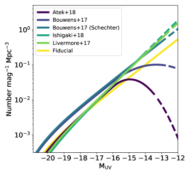
Figure 2: The faint end of the $z\sim 6$ UV luminosity function from Atek et al. (2018), Bouwens et al. (2017), Ishigaki et al. (2018), and Livermore et al. (2017), as well as our fiducial luminosity function (Section 2). In all cases except for the fiducial model, the dashed region of the curves denotes an extrapolation to the observed trend at brighter magnitudes. Atek et al. (2018) and Bouwens et al. (2017) fit for a declining luminosity function above $M_{\mathrm{UV}}$ $=-$16 (also shown is the Schechter function fit to Bouwens et al., 2017). Given their similarity, we will consider the Ishigaki et al. (2018) and Livermore et al. (2017) results together throughout. As discussed in Sections 2 and 6.8, the shape of the faint end of the luminosity function can have a strong effect on the results presented in this work.

Throughout the rest of this work, we will consider the fiducial (Schechter) luminosity function derived above at all redshifts. However, in Section 6.8, we will explore the effect of these different $z\sim 6$ luminosity functions on the number of detectable serendipitous emission line sources.

3 Relationship Between $M_{\mathrm{UV}}$ and Emission Lines

While (UV continuum) luminosity functions predict the number density of galaxies at a given redshift, they do not provide direct constraints on the strength of emission lines, which we require to estimate the number of spectroscopic detection of galaxies. While various studies have concluded that the ‘average’ galaxy at $z\gtrsim 4-6$ has high-EW nebular emission lines (e.g. González et al., 2012; Stark et al., 2013; Labbé et al., 2013; Ceverino et al., 2019), Smit et al. (2016) derive a relationship between $M_{\mathrm{UV}}$ and EW_0,Hα at $z\sim 4.4$. At these redshifts, the strength of H $\alpha$ (plus [N ii] and [S ii]) is determined via a photometric excess in the Spitzer/IRAC photometry. The relation from Smit et al. (2016) is shallow, with a slope $d$ log${}_{10}~{}EW_{0,H\alpha}/dM_{UV}$ of 0.08. To account for the redshift evolution of this relation, we use the result from Labbé et al. (2013), who found that EW_0,Hα increases as $(1+z)^{1.2}$ out to $z\sim 8$. Therefore, we parametrize EW_0,Hα according to:

$$EW_{0,\mathrm{H\alpha}}(M_{\mathrm{UV}},z)=10^{(0.08\times M_{\mathrm{UV}}+4.15)}\left(\frac{1+z}{1+4.4}\right)^{1.2}.$$ (5)

We also incorporate the observed scatter from Smit et al. (2016) into the relation, assuming a Gaussian scatter of $\sigma$ = 0.2 dex. For certain redshifts and $M_{\mathrm{UV}}$ values, the EW value predicted by Equation 5 exceeds 3000 Å, the maximum predicted value from Starburst99 at $Z=0.004$ ($\sim$ 0.25 Z_⊙). In such cases, we adopt this value for EW. This relation is shown in Figure 3.

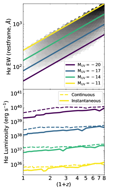
Figure 3: (Top) Relationship between EW_Hα, $M_{\mathrm{UV}}$, and redshift from our model (Equation 5). The background shading shows the (log) density of values for galaxies predicted from our fiducial UV luminosity function (for clarity, only galaxies with $M_{\mathrm{UV}}$ $<-$11 are shown). (Bottom) Predicted H $\alpha$ luminosity versus redshift for the same $M_{\mathrm{UV}}$ values. Our fiducial model with an instantaneous burst of star formation is shown with the solid line while a model using continuous star formation (see Section 6.3 for details) is shown with a dashed line.

While this relationship allows us to predict the EW of H $\alpha$, this does not directly translate into an observable H $\alpha$ flux. Obtaining a line flux from an EW requires knowledge of the continuum level at the position of the line, and the relation between $M_{UV,1550}$ and $M_{6563}$ depends on the stellar population properties. We therefore adopt the models of Starburst99 (Leitherer et al., 1999) to convert EW_0,Hα to $f_{H\alpha}$: we assume an instantaneous burst of star formation with a metallicity $Z=0.004$ and a Salpeter (1955) initial mass function sampled between 1 and 100 M_⊙. With these models, EW_0,Hα maps nearly monotonically to a starburst age. Using this H $\alpha$-derived value for the age of the starburst, the emergent spectrum from the model, normalised to the same $M_{UV,1550}$ as the observed galaxy, is used to estimate the local continuum level at the position of H $\alpha$. This continuum level is then used to convert EW_0,Hα into a line flux.

We would also like to predict the flux of other optical emission lines, namely [O iii] $\lambda$5007. The ratio of H $\alpha$ to [O iii] primarily depends on the metallicity and the ionization parameter and can be as large as 5 in the fiducial photoionization model of Gutkin et al. (2016) at $Z=0.004$. In addition, near-IR grism spectroscopic observations of $1.1<z<2.4$ galaxies with restframe [O iii] EWs in excess of 500 Å by Maseda et al. (2018a), the so-called ‘Extreme Emission Line Galaxies’ (Atek et al., 2011; van der Wel et al., 2011), have an observed ([N ii]-corrected) [O iii]/H $\alpha$ ratio of 2.1 (cf. the value of 1.7 from Anders & Fritze-v. Alvensleben, 2003). These are precisely the types of galaxies that we expect to dominate the population at faint magnitudes and high redshifts and hence dominate the population of serendipitous emission line sources. Therefore, we adopt a value of $f_{\hbox{[O\,{\sc iii}]}}$/$f_{H\alpha}=$ 2.1 $\pm$ 1 (normally-distributed). Further discussion on this point is provided in Section 6.6. For H $\beta$, we assume case B recombination and hence $f_{H\alpha}$/$f_{H\beta}=2.86.$ While we perform the same analysis for H $\beta$ as we do for H $\alpha$ and include its effects in e.g. the contribution to broadband magnitudes in Section 5.1, we do not consider H $\beta$-based detections given its wavelength proximity to the brighter [O iii] emission line.

As we do not consider emission lines apart from [O iii] and H $\alpha$, our results represent a lower limit to the number of potentially observable sources. Another restframe-optical emission line, [O ii] $\lambda\lambda$3727,3729, is commonly observed in star-forming galaxies and would be detectable in NIRSpec up to $z\sim 13$ (currently beyond the constraints from UV luminosity functions based on HST imaging). The ratio of [O iii] to [O ii] varies with ionization parameter, stellar mass, star formation rate, and metallicity (Nakajima & Ouchi, 2014). As such, $z<1$ observations of star-forming galaxies show a mean ratio of 0.4 (Paalvast et al., 2018) whereas the low-mass, low-metallicity $z\sim 2$ ‘Extreme Emission Line Galaxies’ (similar to the sources we expect to dominate the serendipitous NIRSpec counts) have a mean ratio of 3.5 (Maseda et al., 2018a), with evidence that the ratio increases with [O iii] EW (Tang et al., 2018). Hence, large samples of [O ii] emitters might be difficult to obtain at high-$z$. The Williams et al. (2018) JAGUAR catalogue predicts 1/2 as many detectable [O ii] emitters as [O iii] emitters (see Section 6.5). Ly $\alpha$ is also strong in many star-forming galaxies, potentially stronger than H $\alpha$ (e.g. in $z\sim$ 2, 10¹⁰ M_⊙ galaxies; Matthee et al., 2016). However, it is difficult to relate its strength to $M_{\mathrm{UV}}$ in general (e.g. Ando et al., 2006; Nilsson et al., 2009) and it may not be easily observable at $z>6$ where the photons would be absorbed by the predominantly neutral intergalactic medium (e.g. Pentericci et al., 2011; Treu et al., 2012).

4 NIRSpec Observations

NIRSpec offers nine unique spectral configurations spanning the wavelength range 0.6$-$5.3 $\mu$m. This wavelength interval is divided into four wavelength bands (henceforth Bands 0, i, ii, and iii) which are selected via different long-pass filters: $F070LP$, $F100LP$, $F170LP$, and $F290LP$. In each band, specific diffraction gratings can provide $R\sim$ 1000 spectral resolution ($G140M$, $G235M$, and $G395M$) and $R\sim$ 2700 ($G140H$, $G235H$, and $G395H$); Bands 0 and i can be used with either of the G140 gratings. Therefore, Band 0 covers 0.7 $\mu$m $<\lambda<$ 1.3 $\mu$m, Band i covers 1.0 $\mu$m $<\lambda<$ 1.8 $\mu$m, Band ii covers 1.7 $\mu$m $<\lambda<$ 3.1 $\mu$m, and Band iii covers 2.9 $\mu$m $<\lambda<$ 5.3 $\mu$m. NIRSpec’s complete wavelength coverage can be achieved simultaneously with the $R\sim$ 100 prism (and the ‘CLEAR’ blocking filter). A more complete description of NIRSpec’s observation modes can be found in Böker & Tumlinson (2010).

4.1 Instrument sensitivity, slit losses, and spectral resolution

To model the NIRSpec observations we use version 1.3 of the Pandeia (Pontoppidan et al., 2016) code, which is a scriptable exposure time calculator. Pandeia is based on ground test measurements and calibrations of each of JWST’s science instruments. for NIRSpec, Pontoppidan et al. (2016) use data from extensive ground-based cryogenic testing of the instrument science module. They do, however, caution that some uncertainties about the overall throughputs and efficiencies will remain until on-orbit calibrations are performed.

Such caveats notwithstanding, we use Pandeia to determine limiting sensitivities for spatially- and spectrally-unresolved emission lines as a function of wavelength in each possible NIRSpec configuration. We model the observations assuming a 1$\times$3 configuration of open microshutters in the MSA (a ‘microslit’) and a standard three-point nodding pattern in which one third of the total exposure time is spent in each nodding position (centring on shutters $-$1, 0, and +1). In addition, we can model the throughput of the system as a function of spatial position with respect to the open microslit. This can be seen in Figure 4 for the R100 prism observations as the relative throughput for single exposures for for the full three-point nodding pattern.

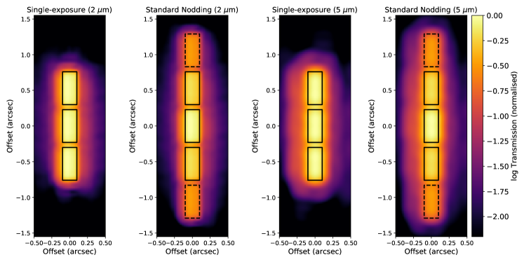
Figure 4: Relative (log) transmission of a point source in R100 (CLEAR/PRISM) mode within a 1$\times$3 NIRSpec microslit (normalised to a centred point source in the central microshutter) as a function of spatial position. Left: the transmission for a single exposure at 2 $\mu$m and for a standard nodding pattern with 1/3 of the exposure time spent with each of the three shutters at the (0,0) position. Right: the same but for 5 $\mu$m. All throughputs are calculated using Pandeia (Pontoppidan et al., 2016). Solid lines denote the original position of the 1$\times$3 NIRSpec microslit while the dashed lines indicate the position of a microshutter in the upper/lower nodding configurations; from top to bottom, each of the five positions observed during a full nodding sequence receives 1/3, 2/3, 1, 2/3, 1/3 of the total exposure time. Particularly at longer wavelengths, objects that lie outside of the 1$\times$3 microslit can have a significant throughput due to the size and wings of the PSF.

Significant throughput in the system occurs even when a (point source) object is not centred inside the open shutter area: an object located 0$\aas@@fstack{\prime\prime}$2 from the microslit centre in the dispersion direction (twice the open area) still has 10 per cent total transmission at 5 $\mu$m. This is a direct consequence of the large wings of the JWST PSF. Asymmetries in the PSF from the telescope and from the NIRSpec optical system lead to variations in the spatial throughput that also vary with wavelength. This is clear from Figure 4 as a gradient in throughput along the dispersion direction at 5 $\mu$m and highlights the need for the full 3D modeling of the instrument transmission performed with Pandeia. Section 6.4 further discusses the impact of the assumption of the source geometry.

In the following we assume the sources are kinematically unresolved, i.e. with velocity widths $\lesssim$ 100 km s^-1, so as not to be resolved even in the highest-resolution mode of NIRSpec ($R\sim$ 2700, otherwise known as R2700). A spectrally-resolved line would lower the S/N estimate slightly by spreading the line flux over more pixels. Typical $z\sim 2$ ‘Extreme Emission Line Galaxies’ have line widths of the order 50 km s^-1 (Maseda et al., 2014) which should anti-correlate with mass. We therefore expect the majority of our serendipitous emission line sources to be spectrally unresolved in all NIRSpec observing modes. Conversely, in R100 spectra [O iii] $\lambda$5007 and $\lambda$4959 are not fully resolved at all wavelengths (see figure 8 of Chevallard et al., 2019). As our model only considers the flux of [O iii] $\lambda$5007 for detections, at $z\lesssim 5$ we may be underestimating the true number of detectable [O iii]-emitters.

4.2 Incomplete wavelength coverage with R2700

While observations with the R100 and R1000 modes can be designed to avoid the gap present between the two NIRSpec detectors, spectra obtained with the R2700 mode are too long ($\approx$3600 pixels) to avoid this gap. By design, only spectra from MSA shutters in the $\sim$200 wide band of columns toward the extreme left edge of the MSA can yield R2700 spectra that cover the full wavelength range (modulo the detector gap). We calculate the effect of the spectral truncation on every operable MSA shutter (193,860 in total) using the MSAViz code (version 1.0.4a2). Results are shown in Figure 5. This effect produces a clear spatial variation, with differences of nearly a factor of two in terms of total wavelength coverage between different parts of the MSA.

Because of this effect, 28 per cent of objects placed in a random microshutter in F290LP/G395H, F170LP/G235H, or F100LP/G140H, (also referred to as R2700 Band iii, Band ii, and Band i, respectively) would lack coverage of H $\alpha$ or [O iii] even though their redshift would imply that the line would be in the nominal wavelength range covered by the configuration. For F070LP/G140H (R2700 Band 0), this number is 13 per cent. When calculating the total number of observable serendipitous sources in each observing mode, we assume this fixed fraction of missing confirmations to average over all possible MSA configurations.

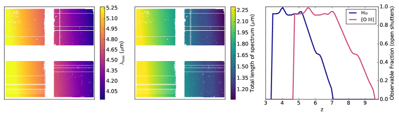
Figure 5: Illustration of the effect of truncated spectra in the R2700 Band iii mode of NIRSpec (nominal: 2.9$-$ 5.3 $\mu$m). Left: the longest wavelength covered for a spectrum beginning at the specified MSA position, as projected onto the detector. Middle: the total length of the R2700 Band iii spectrum, taking into account truncation by the edges of the detectors; only objects in the far left of the MSA have uninterrupted wavelength coverage, excepting the detector gap. Right: total observability of H $\alpha$ and [O iii] emission in R2700 Band iii as a function of redshift when combined over all open MSA shutters. At any spatial position in the MSA, there is not an equal chance that an emission line will be observable. The effect is similar for the other R2700 modes.

5 Expected Numbers of Serendipitous Sources

Our fiducial model for the evolution of the UV luminosity function is used to predict a distribution of line fluxes (H $\alpha$ and [O iii]) based on the method presented in Section 3. For a given exposure time, we calculate the sensitivity of NIRSpec as a function of wavelength for a spectrally-unresolved point source centred in a 1$\times$3 microslit. We then scale this sensitivity as a function of spatial position according to the throughput assuming a standard three-point nodding pattern (Section 4). At each spatial position we determine the fraction of the predicted line emitters that would be detectable ($>$ 5-$\sigma$ in [O iii] and/or H $\alpha$) if the object were located at that position. Note that this ignores (1) the potential spatial extent of the objects, as they are all assumed to be intrinsically point-like and (2) the fact that extracting the flux for an off-centre and potentially newly-discovered source will not necessarily result in the optimal signal-to-noise. The effects of these assumptions are discussed further in Section 6. By taking into account the total volume probed by the NIRSpec microslits, we obtain the total number of observable line emitters per MSA configuration and hence per survey.

Results from a R100 survey as a function of exposure time are shown in Figure 8; objects without broadband detections in HST-based imaging (Figure 8) or JWST-based imaging (Figure 8) will be discussed further in the next section. For four different exposure times (100, 50, 10, and 3 ks), we also show the distribution of redshifts and $M_{\mathrm{UV}}$ values. Longer exposure times result in a larger number of detections at $M_{\mathrm{UV}}$ $\gtrsim-$16. In addition, the largest relative increase comes at redshifts $z=3-6$. Overall, the predicted number of detectable serendipitous sources per microslit exceeds one for an exposure time of 75 ks (21 hours). That is to say, for every targeted source in a NIRSpec R100 observation with 21 hours of exposure time, we expect to see another source with detectable ($>$5-$\sigma$) [O iii] and/or H $\alpha$ emission (cf. Brinchmann et al., 2017).

We can repeat this exercise for different NIRSpec observing modes, taking into account their different 2D transmission functions for their different emission line sensitivities as a function of wavelength. These results are shown in the left panel of Figure 9. At all integration times, the R100 prism is the most efficient at detecting serendipitous sources due to its large wavelength coverage and similar line flux sensitivity to the higher-resolution modes. In general, the two redder settings using the $F290LP$ and $F170LP$ filters (Bands ii and iii) are more efficient than the two bluer settings using $F070LP$ and $F100LP$ (Bands 0 and i) at a fixed exposure time. This is due to the wavelength coverage of the bands and the predominance of $z\gtrsim 3$ [O iii] emitters, visible in the central panel of Figure 8, compared to lower-$z$ emitters at long exposure times. The effect of the incomplete wavelength coverage in the R2700 modes (Section 4.2) is also visible as the nearly constant offset between the dotted and dashed curves since the line flux sensitivities for the medium- and high-resolution gratings are similar, within 7$-$8 per cent on average.

5.1 Serendipitous objects detected in broadband imaging

When designing an MSA configuration for extragalactic spectroscopy in the early years of the mission, many JWST users will likely use CANDELS (Grogin et al., 2011; Koekemoer et al., 2011) HST imaging as the source of their input photometry. CANDELS data covers five well-known extragalactic fields: AEGIS, COSMOS, GOODS-N, GOODS-S, and UDS. The data consists of HST WFC3 and ACS data from the optical to the near-IR. A principle goal of CANDELS-based NIRSpec spectroscopy will be to study the properties of $z\sim 2-6$ galaxies primarily via their restframe-optical emission lines. Given the relative number density of sources in CANDELS, a user might decide to create such a census taking into account the spatial position of other sources in the field, i.e. they will preferentially choose targets with no close companions that could contribute flux inside the microslit.

To estimate the number of serendipitous emission line sources in this case, we follow the same procedure as above. In addition, we apply the criterion that each galaxy must not be visible at HST wavelengths in a survey the depth of CANDELS in GOODS-S (the deepest of the five fields in many ACS and WFC3 filters) using the quoted 5-$\sigma$ values from Skelton et al. (2014) in HST ACS/$F435W$, $F606W$, $F775W$, $F814W$, $F850LP$ and WFC3/$F125W$, $F140W$, $F160W$. An object would be detectable if (1) its UV continuum, based on the $M_{\mathrm{UV}}$ value, is bright enough to be observed directly or (2) the flux of H $\alpha$, [O iii], and/or H $\beta$ would imply that the object is detectable in the broadband imaging. These results are shown in Figure 8.

The most prominent differences with the previous case come when looking at the significantly smaller number of $z\lesssim 2-3$ and $M_{\mathrm{UV}}$ $\lesssim-$18 detections at all exposure times. Filters used in the CANDELS HST imaging contain flux from [O iii] and H $\alpha$ (and H $\beta$) emission up to $z\sim 2.5$, contributing to a number of detections when the EWs are sufficiently large. In addition, the filters probe the UV continuum over the majority of the redshift range in which NIRSpec would detect the emission lines, resulting in a lower number of undetected sources with bright UV magnitudes.

Similar considerations will apply for followup of JWST/NIRCam imaging. Table 1 shows the exposure times and imaging depths achieved (for point sources) in the JWST NIRCam GTO ‘DEEP’ program covering 46 arcmin². Part of this imaging overlaps the Hubble Ultra Deep Field (UDF; Beckwith et al., 2006), one of the most well-studied extragalactic fields, with the deepest HST imaging ever taken. In this region, the combination of HST ACS and WFC3 imaging with NIRCam imaging will be our most complete imaging picture of the distant universe. As above, we can determine the number of serendipitous emission line sources that would be undetectable even in the deepest 4.6 arcmin² of the UDF (using the HST depths from Illingworth et al., 2013, for the JWST/NIRCam depths from Table 1), with results shown in Figure 8. The majority of the sources detectable in exposure times of 10 ks or less are expected to have counterparts in at least one photometric band covered by the UDF and NIRCam ‘DEEP’ surveys. In fact, even at longer exposure times only sources with $M_{\mathrm{UV}}$ $\gtrsim-$16 and $z\gtrsim 4$ remain undetectable with this imaging. The vast majority of these sources (92 per cent) are expected to be detectable via their [O iii] emission. As discussed in Section 6.6, the assumption of a fixed [O iii] to H $\alpha$ ratio equal to 2.1 may be an overestimate in galaxies with extremely low metallicities, which are expected at the highest redshifts and faintest $M_{\mathrm{UV}}$ values. Hence, our predicted counts in this regime likely represent an upper limit.

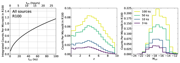
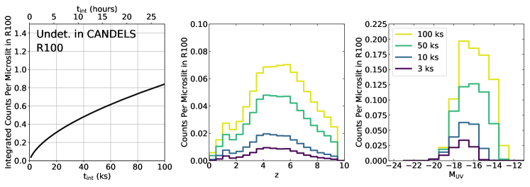
Figure 6: (Left) Estimated cumulative counts of serendipitous emission line sources ($>$5-$\sigma$) in a R100 CLEAR/PRISM survey as a function of the exposure time. (Middle) Redshift distributions for these sources at different exposure times. (Right) M_UV distributions for these sources at different exposure times. The increase in the detectable number of objects with exposure time increases approximately as a power law (deviations no more than 5 per cent) with an exponent of 0.51, implying that surveys become less efficient at detecting these sources with increasing exposure time. The redshift and $M_{\mathrm{UV}}$ distributions, though, do change with exposure time as more high-z ([O iii]) and extremely faint (M${}_{\mathrm{UV}}<$ $-$14) emitters are detectable with longer exposures.

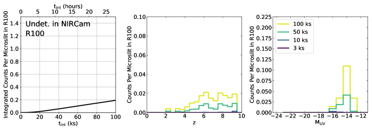
Figure 7: Same as Figure 8 but for sources fainter than the CANDELS GOODS-S detection limits in all applicable HST bands. At a fixed exposure time, brighter ($M_{\mathrm{UV}}$ $<$ $-$19) and lower-$z$ ($z<3$) sources are less common since they are predominantly detectable in the HST imaging.

Figure 8: Same as Figure 8 but for objects which are fainter than the NIRCam ‘DEEP’ survey detection limits (Table 1) and the HST limits in the UDF (Illingworth et al., 2013). Due to the depth and wavelength coverage of NIRCam, many fewer $M_{\mathrm{UV}}$ $<$ $-$16 and $z<4$ galaxies remain even compared to objects that are undetected at CANDELS depth.

Comparisons between all three cases (all objects, objects undetectable in CANDELS imaging, and objects undetectable in the NIRCam ‘DEEP’ survey) are shown in Figure 9 for all NIRSpec configurations. When comparing the shape of the curves, the relation between the integrated counts and the exposure time is nearly a power law for all objects for CANDELS-undetected objects. However, the relationship is noticeably different for the NIRCam-undetected objects. In fact, the derivative d $counts$/ d $t_{int}$ for R100 is constantly decreasing for the former two whereas it increases until $t_{int}=$ 26 ks before flattening for the latter. This implies that the ability to detect serendipitous sources does not increase in efficiency with exposure time when considering all objects or ones that would not be detected in CANDELS-like imaging, and hence the maximal counts would be obtained by a fast tiling of the sky (the contribution of observing overheads notwithstanding). However, for objects that would remain undetectable even in NIRCam imaging, a series of $\sim$7 hour exposures would result in the largest number of serendipitous emission line sources.

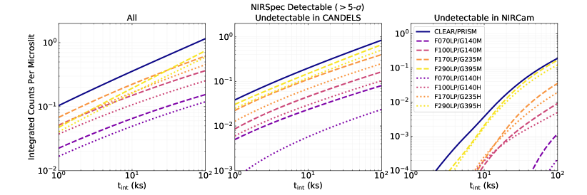
Figure 9: Integrated counts of serendipitous emission line sources ($>$5-$\sigma$, all-$z$) per NIRSpec microslit as a function of exposure time in each grating/filter configuration. The left panel shows the counts for all NIRSpec-detectable sources regardless of their brightness, the middle panel shows the sources that are undetectable at the depth of the CANDELS HST imaging (in GOODS-S), and the right panel shows the sources that are undetectable at the depth of a NIRCam ‘DEEP’ survey (see Table 1). Note the different $y$-scales between the panels.

We can also create a simulated NIRSpec MSA observation by collapsing the projection of 200 individual microslits, approximating a full MSA, along the wavelength direction and combining them into a single 2D map of serendipitous detections, assuming that the sources are distributed randomly on the sky. Figure 10 illustrates this collapsed image for serendipitous H $\alpha$ emitters in the three cases outlined above, with colour-coding in each panel corresponding to $M_{\mathrm{UV}}$, H $\alpha$ flux, and $z$. The same trends as in Figures 8 $-$ 8 manifest themselves in these projections, namely a significantly smaller number of $z\lesssim 4$ and $M_{\mathrm{UV}}$ $\lesssim-$18 sources in the samples of CANDELS- and NIRCam-undetected emitters. The spatial distribution of the sources also changes due to these imaging requirements as the brightest sources with $f_{\mathrm{H\alpha}}>10^{-16}$ erg s^-1 cm^-2, detectable far from the open microslit, would predominantly appear in the broadband imaging. Although our analysis does not consider the potential effect of spatial clustering in the galaxy population, clustering strength decreases with $M_{\mathrm{UV}}$ (Adelberger et al., 2005) and the counts are dominated by faint galaxies.

Considering the small angular separations between some serendipitous sources and the centre of the microslit (Figure 10), it is tantalizing to think that magnification from strong gravitational lensing might allow for the detection of even fainter sources and hence further increase the expected counts. In practice, the incidence rate is difficult to establish as the lensing magnification factor at a fixed angular separation depends on the mass and mass profile of the lensing source, i.e. the primary target of the NIRSpec observations, which are not explicitly considered here. Massive, elliptical galaxies are thought to dominate the total lensing probability of the universe (Turner et al., 1984), so observations targeting these galaxies might result in more detections of lensed background sources. Indeed, two similar instances have been discovered in deep CANDELS HST imaging where an elliptical galaxy at $z=0.65$ strongly lenses an ‘Extreme Emission Line Galaxy’ at $z=1.85$ (Brammer et al., 2012b) and similarly with a lensing elliptical galaxy at $z=1.53$ and an EELG at $z=3.42$ (van der Wel et al., 2013). These observations also highlight the number density of $z>1$ galaxies with high-EW optical emission lines.

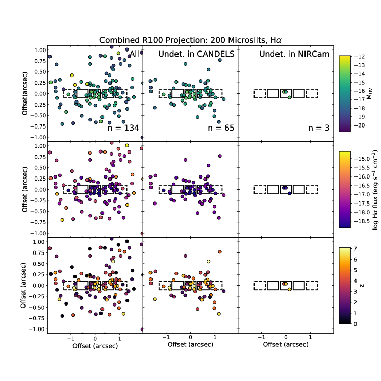
Figure 10: Combined projection of 200 NIRSpec 1$\times$3 microslits (approximating a full MSA) in a 100 ks R100 survey, showing a random iteration of the spatial distribution of serendipitous H $\alpha$ emitters that would be detected at $>$5-$\sigma$ with NIRSpec. The NIRSpec microshutters are shown with the solid and dashed lines (see Figure 4). The sources are colour coded according to the $M_{\mathrm{UV}}$ (top), H $\alpha$ line flux (middle), and redshift (bottom) and split between all observable sources (left; Figure 8), all sources that would be undetectable in CANDELS imaging (middle; Figure 8), and all sources that would be undetectable in NIRCam ‘DEEP’ imaging (right; Figure 8). The same trends as shown in Figures 8 $-$ 8 are clear here, namely the dearth of continuum-bright ($M_{\mathrm{UV}}$ $<$-18) and low-$z$ ($z<2$) sources that would remain undetected in deep photometric data.

NIRCam ‘DEEP’ GTO Imaging
	F090W	F115W	F150W	F200W	F277W	F335M	F356W	F410M	F444W
Exposure time (ks)	60.5	80.8	59.3	38.8	49.1	30.9	38.8	60.5	60.5
5-$\sigma$ Point Source Magnitude (AB)	30.3	30.6	30.7	30.7	30.3	29.6	30.2	29.8	29.9

Table 1: Summary of NIRCam Imaging Program (Proposal ID 1180; PI: D. Eisenstein) covering 46 arcmin². (top) Average exposure times per filter. As pointings often overlap, significantly deeper (2$\times$) regions will exist in the final mosaics. (bottom) The 5-$\sigma$ depth for a point source corresponding to the average exposure times. See also Williams et al. (2018).

6 Discussion

6.1 Comparison to [O iii] in the 3D-HST survey

The large spatial area covered by open microslits in a NIRSpec MSA survey is in many ways similar to a large-field slitless spectroscopic survey. In fact, we can use statistics about the frequency of emission lines in existing slitless (grism) spectroscopic surveys to test our model of emission line fluxes and equivalent widths. The 3D-HST survey (Brammer et al., 2012a; Momcheva et al., 2016), which uses the G141 grism on the HST/Wide Field Camera 3 (WFC3), provides near-complete (modulo contamination) spectral coverage over 626.1 arcmin² from 1.1 to 1.65 microns with a spectral resolution $R\sim 130$.

To compare with 3D-HST, we assume that all emission lines are spectrally- and spatially-unresolved (the latter is explicitly taken into account when determining the limiting sensitivity of the survey; Momcheva et al., 2016). Down to m${}_{F140W}=$ 26.0, 3D-HST has $>$5-$\sigma$ detections of 4972 [O iii] emitters at $1.1<z<2.6$ (Momcheva et al., 2016). Using our model and enforcing the same $F140W$ magnitude limit, we would expect 4474 [O iii] emitters at the same redshifts over the same spatial area, or $\approx$ 10 per cent less than in the full 3D-HST catalogue. We note that this includes objects with low-EW emission lines which are unlikely to be observable at the highest redshifts.

Given that the background noise level in the grism exposures varies by nearly a factor of 3 across the five 3D-HST fields (Brammer et al., 2012a), and that the derived emission line sensitivity is only an average measurement, we conclude that our emission line and equivalent width model is compatible with 3D-HST observations of $1.1<z<2.6$ [O iii] emitters. These data are a close approximation of the JWST/NIRSpec regime at low-$z$.

6.2 Evolution in the model EW with redshift and $M_{\mathrm{UV}}$

In our model for the evolution of H $\alpha$ EW with $z$ and $M_{\mathrm{UV}}$ (Equation 5), we use the redshift evolution from Labbé et al. (2013), EW${}_{\mathrm{H\alpha}}\propto$ (1$+z$)^1.2. This power-law slope implies a factor of $\sim$2 slower evolution than that found in Fumagalli et al. (2012) at $z<2$, EW${}_{\mathrm{H\alpha}}\propto$ (1$+z$)^1.8. Similarly, Mármol-Queraltó et al. (2016) find an even slower evolution, EW${}_{\mathrm{H\alpha}}\propto$ (1$+z$)^1.0. A different evolution with redshift would alter the predictions for the expected number of NIRSpec-detectable serendipitous sources. In particular, we would observe a different number of [O iii] emitters at $z\gtrsim 4-5$, where the observed counts in Figure 8 begin to turn over. In 100 ks at R100, EW${}_{\mathrm{H\alpha}}\propto$ (1$+z$)^1.2 predicts 1.23 detectable ($>$5-$\sigma$) sources per microslit, 0.93 of which would be undetectable at the depth of CANDELS imaging and 0.23 at the depth of the ‘DEEP’ NIRCam imaging; EW${}_{\mathrm{H\alpha}}\propto$ (1$+z$)^1.0 predicts 1.14, 0.82, and 0.17 sources per microslit, respectively (cf. 1.15, 0.84, and 0.19 using our fiducial model).

Only the steeper EW evolution with redshift predicts counts that differ by more than 10 per cent. With this evolution, we would expect a larger number of faint objects (based on the UV luminosity function) to have high-EW emission lines and satisfy these criteria: the difference in EWs between the Fumagalli et al. (2012) evolution and the Labbé et al. (2013) evolution is a factor of 3.7 at $z=8$. As stated previously, the fact that Labbé et al. (2013) base their evolution on measurements that span from $z\sim 1-8$ (or $z=1-5$ for Mármol-Queraltó et al., 2016) compared with just $z\sim 0.6-1.6$ makes it more applicable to high-$z$ studies with NIRSpec.

Similarly, we assume the slope $d~{}\mathrm{log_{10}EW_{H\alpha}}/d~{}M_{\mathrm{UV}}$=0.08 from Smit et al. (2016). This relationship is measured from galaxies with $-$22 $<$ $M_{\mathrm{UV}}$ $<$ $-$20, much brighter than the galaxies that we predict dominate the serendipitous number counts. If we were instead to assume a slope of 0.21 (the 1-$\sigma$ upper limit from Smit et al., 2016), we would expect 2.0 times more serendipitous counts at a fixed $t_{int}$. If there were no relationship (i.e. a slope of 0), then the model predicts 0.6 times the number of serendipitous counts. Thus over a broad range in $d~{}\mathrm{log_{10}EW_{H\alpha}}/d~{}M_{\mathrm{UV}}$, the predicted serendipitous counts can vary by a total factor of 3.1. This is driven by differences at the faint end as the predicted counts at $M_{\mathrm{UV}}$ $>$ $-$18 vary by less than 10 per cent.

The exact slope and scatter of these relations will be robustly constrained in the first large spectroscopic surveys with NIRSpec, as well as large imaging surveys using NIRCam and MIRI.

6.3 Star formation histories

In the conversion of H $\alpha$ EW to H $\alpha$ flux, we could assume a continuous star formation history as opposed to an instantaneous burst. Starburst99 can reproduce the typical H $\alpha$ EWs predicted by our parameterization for a continuous star formation episode of 10$-$100 Myr, similar to the length of star formation episodes in present-day low-mass galaxies ($M_{\star}<$ 10^7.5 M_⊙; Emami et al., 2018) and those predicted by many simulations of galaxy formation at $z>6$ (e.g. Ceverino et al., 2018). As shown in the lower panel of Figure 3, this star formation history results in higher predicted H $\alpha$ luminosities at a fixed EW since the underlying stellar population is older and hence has a brighter optical continuum.

These higher luminosities lead to higher line fluxes and hence a larger number of predicted serendipitous counts. Compared to our fiducial model, a model using continuous star formation predicts 30 per cent more counts at a fixed $t_{int}$. These additional counts are predominantly at $z<6$ (75 per cent of the excess counts) where the H $\alpha$ EWs are lower overall and hence the age difference between the two different star formation histories is largest.

6.4 Physical extent of the serendipitous emitters

In our fiducial model we treat all objects as point-like: a larger source centred inside the microslit would have a lower S/N due to additional slit losses, but non-centred sources would also potentially have more of their flux falling into the microslit. In order to quantify these effects, we consider the case of extended sources with Sérsic indices $n=4$ and $n=1$ and half-light radii of 0$\aas@@fstack{\prime\prime}$2, which is the average projected size of $z=3-6$ galaxies (Shibuya et al., 2015; Curtis-Lake et al., 2016).

If we adopt a fixed 0$\aas@@fstack{\prime\prime}$2 size and Sérsic indices of $n=1$ or $n=4$ instead of a point source geometry for all objects, we predict a larger number of serendipitous counts at a fixed exposure time. The largest number of serendipitous counts is predicted for the $n=4$ Sérsic profile which, for a fixed half-light radius, has the most flux at radii $>$ 1^′′. In general, extended sources have their flux distributed over a larger area and, as most serendipitous counts come from objects that are not located inside the open area of the microslit (Figure 10), this results in significantly more detectable emitters at $z<6$ and $M_{\mathrm{UV}}$ $<-$14. The total counts differ by a factor of 1.64 ($n=4$) and 1.21 ($n=1$) at 100 ks compared to our fiducial model, but this drops to a factor of 1.34 and 1.16, respectively, when restricting to sources with $z>6$ (which are also more likely to be spatially-compact). When restricting to sources with $M_{\mathrm{UV}}$ $>-$14.5, the $n=4$ and $n=1$ counts are lower than the fiducial model by factors of 0.96 and 0.91, respectively, since these faint sources need to be well-centred and a point source geometry results in a higher flux throughput.

Current data, however, indicates that clumpy star formation is more prevalent at high redshifts (e.g. Guo et al., 2015). These clumps do not necessarily have the same emission line properties as the main stellar body of the galaxy (e.g. Zanella et al., 2015) and their surface brightnesses are observed to increase with redshift (Livermore et al., 2015). Therefore a point-source assumption would be appropriate for objects if there is on-average one luminous star-forming clump per galaxy that dominates the line emission of the galaxy; deep JWST/NIRCam imaging probing both the restframe-UV and restframe-optical will shed more light on this issue at the relevant redshifts. Extended sources would also add complications to the detection of these sources as the flux would likely be spread over more detector pixels. Standard methods for background subtraction become more complex with an additional source of flux within a microslit, so observers would need to consider alternatives such as averaging the background level in multiple dedicated sky microslits.

6.5 Comparison to line fluxes in JAGUAR

Chevallard et al. (2019) use BEAGLE (Chevallard & Charlot, 2016) to make predictions for JWST observations based on existing photometric samples in the UDF, modeling and predicting the radiation coming from realistic stellar populations and the effects on the gas within the galaxy. Williams et al. (2018) take this analysis further by creating a full ‘mock’ catalogue (‘JAGUAR’) of sources based on existing mass and luminosity functions, with extrapolations to higher redshifts, lower masses, and lower luminosities than are currently constrained with observations. This includes information about the broadband SEDs of the galaxies for predictions for the fluxes of various emission lines.

Figure 11 compares our method for obtaining H $\alpha$ EWs from the UV luminosity (right panels) to the JAGUAR EWs from Williams et al. (2018, left panels). The mean ratio of the JAGUAR H $\alpha$ EW and the $M_{\mathrm{UV}}$-derived EW is 0.78 for galaxies of all magnitudes. As can be seen, the distribution of EWs does not match the relationship between EW and redshift derived in Labbé et al. (2013). However, when restricting to the same $M_{\mathrm{UV}}$ range as Labbé et al. (2013, i.e. $M_{\mathrm{UV}}$ $<-$20.5), then the distribution of both JAGUAR and $M_{\mathrm{UV}}$-derived EWs with redshift matches well (bottom panels). In particular, the agreement in the bottom-right panel highlights the agreement between the observations of Labbé et al. (2013) and those of Smit et al. (2016), both of which are used to derive Equation 5 and both of which rely on photometric excesses in IRAC data to measure optical line EWs at $z>4$.

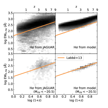
Figure 11: H $\alpha$ EW versus redshift for the full Williams et al. (2018) JAGUAR catalogue (top-left) and from the prediction based on $M_{\mathrm{UV}}$ (Equation 5, top-right) with (log) density in each bin shown with shading. The relationship from Labbé et al. (2013) is overplotted as the solid line and appears to under-predict the H $\alpha$ EWs at all redshifts. However, as noted in Section 3, there is a dependence on $M_{\mathrm{UV}}$: Labbé et al. (2013) only measure EWs in galaxies above 1.5 M^∗ at $z=8$, corresponding to $M_{\mathrm{UV}}$ $=-$20.5. When we restrict the JAGUAR catalogue to values brighter than this, we obtain a better agreement (bottom panels).

Williams et al. (2018) use this catalogue to predict the number counts of high-$z$ galaxies in NIRCam surveys, but it can also be used to predict the number of serendipitous sources that would be detectable with NIRSpec. To determine the number of serendipitous sources from this catalogue, we place a series of 10,000 microslits in random positions within the JAGUAR catalogue field-of-view. We then apply the NIRSpec throughputs (Figure 4) to mimic an observation and nodding sequence and determine how many objects would have their H $\alpha$ and/or [O iii] emission detected as a function of the total exposure time. The catalogue also contains HST and JWST broadband fluxes for each object (including the contribution of the emission lines) so CANDELS and NIRSpec ‘DEEP’ detectability are, as before, defined to be any broadband magnitude greater than the nominal 5-$\sigma$ survey limit in that band.

Results for R100 are illustrated in Figure 12, also including the model predictions from Figures 8 $-$ 8. The predicted H $\alpha$ counts (top panel) are comparable to within a factor of $\times$1.4 for the total number as well as for the CANDELS-undetected objects and within a factor of $\times$5 for NIRCam-undetected objects. The predictions for [O iii] counts differ by a larger amount: a factor of $\times$2.4 and $\times$5.3 for the total number and the CANDELS-undetected objects and a factor of $\times$200 for the NIRCam-undetected objects (solid lines; lower panel). If we were to assume a lower EW for [O iii], specifically setting the flux to be equal to that of H $\alpha$, we obtain the dashed curves which agree with the JAGUAR catalogue results similarly to the case of H $\alpha$.

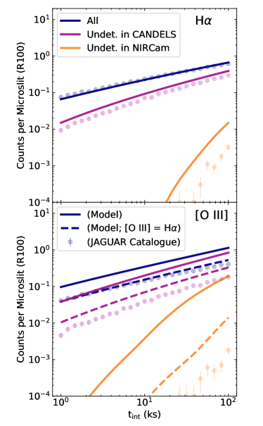
Figure 12: Comparison of the estimated counts of NIRSpec-detectable ($>$5-$\sigma$) serendipitous sources from our model (solid lines) and from simulated observations from the JAGUAR catalogue of Williams et al. (2018, poisson counting errors included); the top panel is for H $\alpha$ emitters and the bottom panel is for [O iii] emitters. Colours differentiate the three different regimes: all galaxies (blue), sources undetectable in CANDELS imaging (purple), and sources undetectable in NIRCam ‘DEEP’ imaging (orange). The counts for [O iii] are noticeably higher in the model than in the JAGUAR catalogue as we assume a higher average value for [O iii]/H $\alpha$, but when setting the fluxes of the lines to be the same the agreement is much better (dashed lines, bottom panel).

In general, the predictions from the JAGUAR catalogue and from our $M_{\mathrm{UV}}$-based model agree well for H $\alpha$ and we can understand the discrepancy for [O iii] due to differences in the relative strength of that emission line. We will discuss the strength of [O iii] in the next section. Nevertheless, this comparison shows that we do expect significant numbers of serendipitous emission line sources in deep NIRSpec observations, even when considering H $\alpha$ alone. The slopes of the relations (d counts / d $t_{int}$) from the model and from JAGUAR are strikingly similar even when the normalisations are different. This similarity further reinforces our model relating emission line strength to the UV continuum luminosity functions, which rise as a power-law at the faint end where the majority of the serendipitous sources lie.

6.6 Dependence on the [O iii] to H $\alpha$ ratio

As mentioned in Section 3, we adopt a median ratio of [O iii] to H $\alpha$ of 2.1 This is slightly higher than what is assumed in e.g. Anders & Fritze-v. Alvensleben (2003), which results from our use of observational constraints from emission line-dominated galaxies at $z\sim 2$ as well as different stellar population models. Specifically, we use the models of Gutkin et al. (2016) at $Z=0.004$ which were specifically designed to reproduce nebular emission in galaxies that span a broad range in physical properties and redshifts. These models do not completely rely on calibrations from Hii regions and local galaxies which do not necessarily represent the range in physical conditions expected in the average galaxy at high redshift (e.g. Brinchmann et al., 2008; Erb et al., 2010; Stark et al., 2014; Shapley et al., 2015; Sanders et al., 2016; Strom et al., 2017; Chevallard et al., 2018). Dust is not explicitly included in our model, which would also lower the observed [O iii]/H $\alpha$ ratio from the intrinsic ratio. However, dust attenuation is not expected to contribute strongly at low masses (Garn & Best, 2010; Schaerer & de Barros, 2010) and specifically for $z\gtrsim 1$ galaxies with high-EW optical emission lines (Maseda et al., 2014).

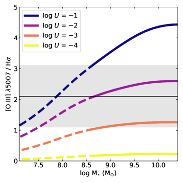
Figure 13: Ratio of [O iii] $\lambda$5007 to H $\alpha$ versus stellar mass from the Gutkin et al. (2016) for different log $U$ values and assuming the mass-metallicity relation from Amorín et al. (2010), with the shaded region showing our 1-$\sigma$ adopted value of 2.1 $\pm$ 1. The chosen mass metallicity relation is measured for ‘Extreme Emission Line Galaxies’ at $z\sim 0.3$, with dashed portions of the lines representing extrapolations to lower masses. Galaxies with intense radiation fields (log $U\gtrsim-2$; Amorín et al., 2014) are expected to contribute the most to the serendipitous counts, although at extremely low masses and metallicities the number of [O iii] detections could begin to drop.

As a result of using this ratio, we predict more detectable [O iii] emitters than the Williams et al. (2018) JAGUAR catalogue described in the previous section (when using [O iii]/H $\alpha$ $=$ 1, we obtain the dashed curves in Figure 12, which provides better agreement with the JAGUAR catalogue). This ratio changes with galaxy properties such as metallicity and ionization parameter (Harikane et al., 2018) which in turn evolve with redshift, and hence our fixed ratio represents a simplification of the true emission line properties of high-$z$ galaxies. This ratio is predicted to drop at the lowest metallicities (and hence stellar masses), but the mass at which this happens depends on the exact mass-metallicity relationship assumed and this regime is not yet observed. Figure 13 shows how this ratio evolves with stellar mass (via the mass-metallicity relationship) and log $U$ for the Gutkin et al. (2016) models assuming $\xi_{d}=0.3$, $n_{H}=100$ cm^-3, C/O = C/O_⊙, and $m_{up}=100$ M_⊙. While the $z\sim 0.3$ mass-metallicity relationship for ‘Extreme Emission Line Galaxies’ (Amorín et al., 2010) is the closest proxy for the types of galaxies we expect to be producing strong emission lines at high-$z$; even assuming the relation from Troncoso et al. (2014) at $z\approx 3.5$ for all star-forming galaxies produces similar evolution in the ratio at masses $>$ 10^7.5 M_⊙. Observations of these emission line-dominated galaxies imply log $U\approx-2$ to $-1$ (Erb et al., 2010; Amorín et al., 2014; Berg et al., 2018) which is much larger than the values for local star-forming galaxies used in Williams et al. (2018) based on the observations of Carton et al. (2017). This is also true for the general population of [O iii]-emitting galaxies at $z>3$, which have higher ionization parameters at fixed stellar mass or metallicity than locally (Suzuki et al., 2017).

The true distribution of this ratio will not be known until JWST/NIRSpec assembles large samples of high-$z$ galaxies with detections of both lines. Our simple model uses a ratio based on observations of [O iii] and H $\alpha$ in high-EW (high specific star formation rate), low-metallicity ($<$ 25 per cent Z_⊙), 10^8-9 M_⊙ galaxies at $z\sim 1-2.5$ (Maseda et al., 2018a) which have similar [O iii] and H $\alpha$ equivalent widths to the galaxies that we expect to be serendipitously detectable with NIRSpec. While the agreement between the predictions and the 3D-HST observations described in Section 6.1 gives observational evidence at $z\approx 2$ for our assumption about the ratio of [O iii] to H $\alpha$, the relationship between emission line-dominated objects and the general population of star-forming galaxies at higher redshifts remains to be seen. In the most pessimistic case where [O iii] is never detected because it is intrinsically much fainter than H $\alpha$, our predicted counts would be given by the curves in the upper panel of Figure 12 where we would still achieve 0.67 counts per open microslit in 100 ks.

6.7 Serendipitous versus targeted counts at high-$z$

Given the expected number of serendipitous $z\gtrsim 6$ galaxies observable in a NIRSpec survey (see Figure 8), it is natural to ask if the overall number counts of such high-$z$ galaxies will be dominated by serendipitous discoveries or by targeted spectroscopy. This high-redshift frontier represents one of the key aspects of the JWST mission in general and specifically one of the drivers for approved GTO and ERS programs.

As mentioned above, Bouwens et al. (2015) detect 137 $z>6$ photometric dropout candidates in the deep-WFC3 area UDF (123 $\times$ 136 arcsec). This implies a source density of 29.5 objects per arcminute². According to Jakobsen (2017), the average maximum number of non-overlapping R100 spectra at this source density is 65. In practice, this is an overestimate given that the objects are distributed over an area much smaller than the full NIRSpec field-of-view. Nevertheless, 65 $z>6$ spectra is still less than the 78 (0.39 per microslit) we would expect to serendipitously detect in a deep MSA survey with 200 open microslits at 100 ks.

The 11 $\times$ 11 arcminute JWST JAGUAR catalogue of Williams et al. (2018) contains 9355 $z>6$ galaxies with UV magnitudes that would make them detectable in the DEEP component of the NIRCam/NIRSpec joint GTO program (see Table 1), implying a source density of 77 objects per arcminute² or 110 non-overlapping R100 spectra per MSA configuration (Jakobsen, 2017). In the area of the deepest planned NIRSpec observations (Proposal ID 1210; PI: P. Ferruit) of 100 ks, covering the UDF as followup of the NIRCam DEEP observations, we would therefore expect similar numbers of serendipitous $z>6$ and targeted detections.

6.8 Effect of the faint end of the UV luminosity function

Given the discussion in the literature about the faint-end shape of the UV luminosity function at $z\sim 6$, we consider the effect that such differences would have on the observable number of serendipitous emission line sources. To do so we perform calculations as before, but instead of our fiducial (Schechter) luminosity function we use the Atek et al. (2018) and Bouwens et al. (2017) luminosity functions, which include a departure from a power-law at $M_{\mathrm{UV}}$ $<-$16, and the Schechter function fits from Livermore et al. (2017) and Ishigaki et al. (2018). The last two power-law luminosity functions produce observable counts that are similar within 5 per cent, so for the purposes of this work we consider them as a single luminosity function.

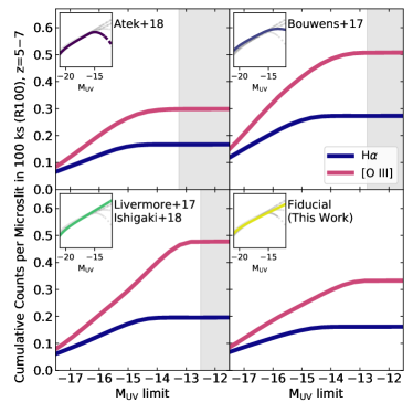
Figure 14: Cumulative number counts per microslit of predicted observable H $\alpha$- and [O iii]-emitters at $z=5-7$ from a 100 ks R100 survey as a function of the faint $M_{\mathrm{UV}}$ limit to which the luminosity function is probed. Each panel shows the results for a different UV luminosity function: the top panels show the predictions for the Atek et al. (2018) and Bouwens et al. (2017) luminosity functions, which include a departure from a power-law at $M_{\mathrm{UV}}$ $=-$16; the bottom panels show the predictions for Livermore et al. (2017); Ishigaki et al. (2018) and our fiducial model (Section 2) for power-law slopes to the faintest magnitudes. The shaded grey regions denote the observational limit to each luminosity function. Large samples of serendipitous [O iii] and H $\alpha$ emitters at these redshifts can, in conjunction with deep imaging data, constrain the shape and potential $M_{\mathrm{UV}}$ cutoff of the UV luminosity function.

Results for H $\alpha$ and [O iii] counts as a function of the faint end of the UV luminosity function are shown in Figure 14. Using the Bouwens et al. (2017) luminosity function results in the largest predicted number of emitters (0.50 [O iii] emitters and 0.27 H $\alpha$ emitters per microslit) if the luminosity function extends to at least $M_{\mathrm{UV}}$ $=-$12, with comparable results for the Livermore et al. (2017) and Ishigaki et al. (2018) luminosity function. Using the Atek et al. (2018) luminosity function results in the fewest (0.30 [O iii] emitters and 0.17 H $\alpha$ emitters).

While UV luminosity functions obtained from deep NIRCam imaging will help to resolve this question (e.g. Yung et al., 2018), NIRSpec will also be crucial in providing spectroscopic confirmations. As the UV luminosity function needs to extend to at least $M_{\mathrm{UV}}$ $\sim-$13 at $z\sim 7-9$ in order for galaxies to reionize the universe (e.g. Robertson et al., 2013), serendipitous detections with NIRSpec could provide valuable constraints on the number counts of such galaxies considering not all $M_{\mathrm{UV}}$ $>-$14 sources will be detectable even with the deepest NIRCam imaging (Figure 8). In fact, the Williams et al. (2018) JAGUAR catalogue does not contain any galaxies at $z>6$ with $M_{\mathrm{UV}}$ $>-$14 that would be detectable in the ‘DEEP’ NIRCam imaging (cf. their figure 25). However, our model predicts NIRSpec confirmations for 0.07 objects per open microslit at $z>6$ with $M_{\mathrm{UV}}$ $>-$14 in 100 ks at R100, and even 0.01 at $z>6$ with $M_{\mathrm{UV}}$ $>-$13. This is also visible in Figure 15, where serendipitous counts with $M_{\mathrm{UV}}$ $>-$14 become more prevalent at $z>4$ (top panel).

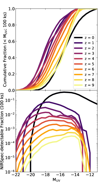
Figure 15: (Top) Cumulative fraction of NIRSpec-detectable ($>$5-$\sigma$) galaxies in a 100 ks R100 observation as a function of $M_{\mathrm{UV}}$ and $z$. (Bottom) Total non-cumulative fraction of objects at a given $M_{\mathrm{UV}}$ and $z$, based on our fiducial luminosity function, that have H $\alpha$ or [O iii] detectable in a 100 ks R100 observation. While the lower-$z$ objects have a higher detectable fraction, the larger numbers of higher-$z$ galaxies mean that they dominate the total counts, as seen in Figure 8. At $z>5$, we also see that the majority of detections occur at $M_{\mathrm{UV}}$ $\gtrsim$ $-$17.

Deep (blind) NIRSpec exposures may therefore represent the most efficient way to find the faintest galaxies at high-$z$. Confirming the UV magnitudes may be difficult when they are not detected in the broadband imaging, but a large enough sample could be stacked together to obtain an average measurement, as in Maseda et al. (2018b). In fact, such confirmations might serve as an independent (spectroscopic-based) constraint on the faint end of the high-$z$ UV luminosity function. At these faint magnitudes, NIRSpec detections are likely to make up only a low fraction of the total number of galaxies at high-$z$, $\sim$0.01 per cent (Figure 15) highlighting the difficulty of studying the average properties of the sources likely responsible for reionization even with JWST.

7 Conclusions

In this work, we predict the number counts of emission line sources that are serendipitously detectable in the multi-object spectroscopy mode of JWST’s NIRSpec instrument. To do so, we develop a model that relates the fluxes and EWs of the H $\alpha$ and [O iii] emission lines to the $M_{\mathrm{UV}}$ and redshift of the galaxy. When coupled to a UV luminosity function that evolves smoothly with redshift, this predicts the line flux distributions of galaxies at a given redshift. With no a priori knowledge of the spatial location of these objects, we calculate the effective volume that NIRSpec probes as a function of the limiting detectable flux in a standard observing setup; even off-centre sources can have much of their flux enter through an open microslit. This model therefore produces the following results:

• For integration times greater than 21 hours (75 ks) in the R100 mode, NIRSpec will serendipitously detect at least one H $\alpha$ and/or [O iii] emitter with $>$5-$\sigma$ significance per open microslit, i.e. there will be an equal or greater number of serendipitous sources than primary targets (Figure 8). At exposure times greater than 6 hours (20 ks), we predict at least 0.5 ($>$5-$\sigma$) emitters per microslit. If we restrict to only H $\alpha$ detections (e.g. if [O iii] is much fainter than our model predicts), then we predict 0.67 detections per open microslit in 100 ks.

• When considering objects that could be detected in broadband imaging, the expected number of serendipitous sources decreases at a fixed integration time depending on the type and depth of the imaging considered. In this work, we consider HST-based imaging as in the CANDELS GOODS-S field as well as the combination of HST-based and JWST/NIRCam-based ‘DEEP’ imaging in the UDF (Figures 8 and 8).

• The R100 mode of NIRSpec, with full spectral coverage from 0.6 to 5.3 $\mu$m, is the most efficient observing mode for detecting serendipitous sources at all exposure times (Figure 9).

• The model predicts NIRSpec detections in some $M_{\mathrm{UV}}$ $>-14$ galaxies, 92 per cent of which are [O iii] emitters assuming our fiducial [O iii] to H $\alpha$ ratio, which might not be detectable even in the deepest NIRCam imaging to be taken with JWST in blank fields (Figures 8 and 15). Detections in such faint galaxies would represent an independent way to constrain the faint end of the high-$z$ UV luminosity functions (Figure 14).

Given the number of potential open microslits in the NIRSpec MSA, surveys intending to optimize number counts of emission line galaxies should strive to open as many as possible in any configuration.

Appendix A UV Luminosity Functions

$<z>$	$\alpha$	log $\phi_{\star}$	M⋆	Reference
0.3	$-$1.19$\pm$0.15	$-$2.21$\pm$0.12	$-$18.38$\pm$0.25	Arnouts et al. (2005)
0.5	$-$1.55$\pm$0.21	$-$2.77$\pm$0.23	$-$19.49$\pm$0.37	Arnouts et al. (2005)
0.7	$-$1.60$\pm$0.26	$-$2.78$\pm$0.25	$-$19.84$\pm$0.40	Arnouts et al. (2005)
1.0	$-$1.63$\pm$0.45	$-$2.94$\pm$0.29	$-$20.11$\pm$0.45	Arnouts et al. (2005)
0.05	$-$1.22$\pm$0.07	$-$2.37$\pm$0.06	$-$18.04$\pm$0.11	Wyder et al. (2005)
1.7	$-$0.81$\pm$0.18	$-$1.77$\pm$0.11	$-$19.80$\pm$0.29	Sawicki & Thompson (2006)
3.0	$-$1.43$\pm$0.13	$-$2.77$\pm$0.11	$-$20.90$\pm$0.18	Sawicki & Thompson (2006)
4.0	$-$1.26$\pm$0.38	$-$3.07$\pm$0.27	$-$21.00$\pm$0.43	Sawicki & Thompson (2006)
4.0	$-$1.82$\pm$0.09	$-$2.84$\pm$0.11	$-$21.14$\pm$0.15	Yoshida et al. (2006)
4.7	$-$2.31$\pm$0.64	$-$3.24$\pm$0.58	$-$21.09$\pm$0.64	Yoshida et al. (2006)
1.14	$-$1.48$\pm$0.32	$-$2.53$\pm$0.02	$-$19.62$\pm$0.06	Dahlen et al. (2007)
1.75	$-$1.48$\pm$0.32	$-$2.51$\pm$0.23	$-$20.24$\pm$0.32	Dahlen et al. (2007)
2.23	$-$1.48$\pm$0.32	$-$2.48$\pm$0.13	$-$19.87$\pm$0.18	Dahlen et al. (2007)
4.8	$-$1.48$\pm$0.35	$-$3.39$\pm$0.31	$-$21.28$\pm$0.38	Iwata et al. (2007)
6.9	$-$1.72$\pm$0.65	$-$3.16$\pm$1.00	$-$20.10$\pm$0.76	Ouchi et al. (2009)
5.0	$-$1.66$\pm$0.06	$-$3.03$\pm$0.09	$-$20.73$\pm$0.11	McLure et al. (2009)
6.0	$-$1.71$\pm$0.11	$-$2.74$\pm$0.12	$-$20.04$\pm$0.12	McLure et al. (2009)
2.3	$-$1.73$\pm$0.07	$-$2.56$\pm$0.09	$-$20.70$\pm$0.11	Reddy & Steidel (2009)
3.05	$-$1.73$\pm$0.13	$-$2.77$\pm$0.13	$-$20.97$\pm$0.14	Reddy & Steidel (2009)
1.7	$-$1.27	$-$2.66$\pm$0.15	$-$19.43$\pm$0.36	Hathi et al. (2010)
2.1	$-$1.17$\pm$0.40	$-$2.80$\pm$0.32	$-$20.39$\pm$0.64	Hathi et al. (2010)
2.7	$-$1.52$\pm$0.29	$-$2.81$\pm$0.32	$-$20.94$\pm$0.53	Hathi et al. (2010)
1.5	$-$1.46$\pm$0.54	$-$2.64$\pm$0.33	$-$19.82$\pm$0.51	Oesch et al. (2010)
1.9	$-$1.60$\pm$0.51	$-$2.66$\pm$0.36	$-$20.16$\pm$0.52	Oesch et al. (2010)
2.5	$-$1.73$\pm$0.11	$-$2.49$\pm$0.12	$-$20.69$\pm$0.17	Oesch et al. (2010)
3.1	$-$1.65$\pm$0.12	$-$2.75$\pm$0.11	$-$20.94$\pm$0.14	van der Burg et al. (2010)
3.8	$-$1.56$\pm$0.08	$-$2.87$\pm$0.07	$-$20.84$\pm$0.09	van der Burg et al. (2010)
4.8	$-$1.65$\pm$0.09	$-$3.08$\pm$0.08	$-$20.94$\pm$0.11	van der Burg et al. (2010)
8.0	$-$1.98$\pm$0.23	$-$-3.37$\pm$0.28	$-$20.26$\pm$0.32	Bradley et al. (2012)
0.13	$-$1.05$\pm$0.04	$-$2.15$\pm$0.03	$-$18.12	Cucciati et al. (2012)
0.3	$-$1.17$\pm$0.05	$-$2.16$\pm$0.06	$-$18.30$\pm$0.15	Cucciati et al. (2012)
0.5	$-$1.07$\pm$0.07	$-$2.18$\pm$0.06	$-$18.40$\pm$0.10	Cucciati et al. (2012)
0.7	$-$0.90$\pm$0.08	$-$2.02$\pm$0.05	$-$18.30$\pm$0.10	Cucciati et al. (2012)
0.9	$-$0.85$\pm$0.10	$-$2.05$\pm$0.05	$-$18.70$\pm$0.10	Cucciati et al. (2012)
1.1	$-$0.91$\pm$0.16	$-$2.13$\pm$0.07	$-$19.00$\pm$0.20	Cucciati et al. (2012)
1.5	$-$1.09$\pm$0.23	$-$2.39$\pm$0.09	$-$19.60$\pm$0.20	Cucciati et al. (2012)
2.1	$-$1.30	$-$2.47$\pm$0.03	$-$20.40$\pm$0.10	Cucciati et al. (2012)
3.0	$-$1.50	$-$3.07$\pm$0.03	$-$21.40$\pm$0.10	Cucciati et al. (2012)
4.0	$-$1.73	$-$3.96$\pm$0.04	$-$22.20$\pm$0.20	Cucciati et al. (2012)
2.2	$-$1.47$\pm$0.23	$-$2.74$\pm$0.32	$-$21.00$\pm$0.55	Sawicki (2012)
7.0	$-$1.90$\pm$0.15	$-$2.96$\pm$0.21	$-$19.90$\pm$0.26	McLure et al. (2013)
8.0	$-$2.02$\pm$0.23	$-$3.35$\pm$0.38	$-$20.12$\pm$0.43	McLure et al. (2013)
7.0	$-$1.87$\pm$0.18	$-$3.19$\pm$0.26	$-$20.14$\pm$0.42	Schenker et al. (2013)
8.0	$-$1.94$\pm$0.23	$-$3.50$\pm$0.34	$-$20.44$\pm$0.41	Schenker et al. (2013)
2.0	$-$1.74$\pm$0.08	$-$2.54$\pm$0.15	$-$20.01$\pm$0.24	Alavi et al. (2014)
8.0	$-$2.08$\pm$0.30	$-$-3.51$\pm$0.44	$-$20.40$\pm$0.47	Schmidt et al. (2014)
0.75	$-$1.23$\pm$0.11	$-$2.45$\pm$0.53	$-$18.62$\pm$0.24	Weisz et al. (2014)
1.25	$-$1.19$\pm$0.11	$-$2.83$\pm$0.38	$-$18.97$\pm$0.22	Weisz et al. (2014)
2.0	$-$1.36$\pm$0.14	$-$2.89$\pm$0.98	$-$19.36$\pm$0.33	Weisz et al. (2014)
3.0	$-$1.36$\pm$0.13	$-$3.00$\pm$0.63	$-$20.45$\pm$0.23	Weisz et al. (2014)
4.0	$-$1.58$\pm$0.08	$-$4.22$\pm$0.80	$-$20.89$\pm$0.13	Weisz et al. (2014)
5.0	$-$1.57$\pm$0.11	$-$4.22$\pm$1.81	$-$20.83$\pm$0.17	Weisz et al. (2014)
3.8	$-$1.64$\pm$0.04	$-$2.71$\pm$0.07	$-$20.88$\pm$0.08	Bouwens et al. (2015)
4.9	$-$1.76$\pm$0.06	$-$3.10$\pm$0.11	$-$21.10$\pm$0.15	Bouwens et al. (2015)
5.9	$-$1.90$\pm$0.10	$-$3.41$\pm$0.19	$-$21.10$\pm$0.24	Bouwens et al. (2015)
6.8	$-$1.98$\pm$0.15	$-$3.34$\pm$0.28	$-$20.61$\pm$0.31	Bouwens et al. (2015)
7.9	$-$1.81$\pm$0.27	$-$3.36$\pm$0.38	$-$20.19$\pm$0.42	Bouwens et al. (2015)
10.4	$-$2.27	$-$4.89$\pm$0.20	$-$20.92	Bouwens et al. (2015)
5.9	$-$1.88$\pm$0.15	$-$3.24$\pm$0.18	$-$20.77$\pm$0.19	Bowler et al. (2015)

Table 2: UV luminosity functions considered in this work. In cases where asymmetric errors are reported, we include the average (symmetrized) errors; when no error is reported, we assume an error of 0.5.

Table 3: continued

UV luminosity functions considered in this work. $<z>$ $\alpha$ log $\phi_{\star}$ M_⋆ Reference 4.0 $-$1.56$\pm$0.06 $-$2.85$\pm$0.06 $-$20.73$\pm$0.09 Finkelstein et al. (2015) 5.0 $-$1.67$\pm$0.06 $-$3.05$\pm$0.08 $-$20.81$\pm$0.13 Finkelstein et al. (2015) 6.0 $-$2.02$\pm$0.10 $-$3.73$\pm$0.20 $-$21.13$\pm$0.28 Finkelstein et al. (2015) 7.0 $-$2.03$\pm$0.21 $-$3.80$\pm$0.34 $-$21.03$\pm$0.44 Finkelstein et al. (2015) 8.0 $-$2.36$\pm$0.47 $-$4.14$\pm$0.96 $-$20.89$\pm$0.91 Finkelstein et al. (2015) 9.0 $-$2.02 $-$3.60$\pm$0.23 $-$20.1 McLeod et al. (2015) 1.3 $-$1.56$\pm$0.04 $-$2.63$\pm$0.09 $-$19.74$\pm$0.18 Alavi et al. (2016) 1.9 $-$1.72$\pm$0.04 $-$2.82$\pm$0.11 $-$20.41$\pm$0.20 Alavi et al. (2016) 2.6 $-$1.94$\pm$0.06 $-$3.26$\pm$0.11 $-$20.71$\pm$0.11 Alavi et al. (2016) 7.0 $-$1.91$\pm$0.27 $-$3.43$\pm$0.13 $-$20.33$\pm$0.42 Laporte et al. (2016) 8.0 $-$1.95$\pm$0.42 $-$3.52$\pm$0.75 $-$20.32$\pm$0.38 Laporte et al. (2016) 9.0 $-$2.17$\pm$0.42 $-$4.15$\pm$0.19 $-$20.45 Laporte et al. (2016) 1.7 $-$1.33$\pm$0.03 $-$2.17$\pm$0.05 $-$19.61$\pm$0.07 Parsa et al. (2016) 1.9 $-$1.32$\pm$0.03 $-$2.15$\pm$0.04 $-$19.68$\pm$0.05 Parsa et al. (2016) 2.25 $-$1.26$\pm$0.04 $-$2.12$\pm$0.05 $-$19.71$\pm$0.07 Parsa et al. (2016) 2.8 $-$1.31$\pm$0.04 $-$2.27$\pm$0.05 $-$20.20$\pm$0.07 Parsa et al. (2016) 3.8 $-$1.43$\pm$0.04 $-$2.69$\pm$0.07 $-$20.71$\pm$0.10 Parsa et al. (2016) 5.9 $-$1.91$\pm$0.03 $-$3.19$\pm$0.04 $-$20.94 Bouwens et al. (2017) 6.0 $-$2.10$\pm$0.03 $-$3.65$\pm$0.04 $-$20.83$\pm$0.05 Livermore et al. (2017) 7.0 $-$2.06$\pm$0.04 $-$3.67$\pm$0.04 $-$20.80$\pm$0.05 Livermore et al. (2017) 8.0 $-$2.01$\pm$0.08 $-$3.77$\pm$0.13 $-$20.72$\pm$0.16 Livermore et al. (2017) 7.0 $-$1.98$\pm$0.10 $-$3.43$\pm$0.21 $-$20.74$\pm$0.21 Atek et al. (2018) 6.5 $-$2.15$\pm$0.07 $-$3.78$\pm$0.15 $-$20.89$\pm$0.15 Ishigaki et al. (2018) 8.0 $-$1.96$\pm$0.17 $-$3.60$\pm$0.23 $-$20.35$\pm$0.25 Ishigaki et al. (2018) 9.0 $-$1.96 $-$3.88$\pm$0.10 $-$20.35 Ishigaki et al. (2018) 10.0 $-$1.96 $-$4.60$\pm$0.18 $-$20.35 Ishigaki et al. (2018) 10.0 $-$2.28$\pm$0.32 $-$4.89$\pm$0.27 $-$20.60 Oesch et al. (2018)

References

- Adelberger et al. (2005) Adelberger K. L., Steidel C. C., Pettini M., Shapley A. E., Reddy N. A., Erb D. K., 2005, ApJ, 619, 697
- Alavi et al. (2014) Alavi A., et al., 2014, ApJ, 780, 143
- Alavi et al. (2016) Alavi A., et al., 2016, ApJ, 832, 56
- Amorín et al. (2010) Amorín R. O., Pérez-Montero E., Vílchez J. M., 2010, ApJ, 715, L128
- Amorín et al. (2014) Amorín R., et al., 2014, ApJ, 788, L4
- Anders & Fritze-v. Alvensleben (2003) Anders P., Fritze-v. Alvensleben U., 2003, A&A, 401, 1063
- Ando et al. (2006) Ando M., Ohta K., Iwata I., Akiyama M., Aoki K., Tamura N., 2006, ApJ, 645, L9
- Arnouts et al. (2005) Arnouts S., et al., 2005, ApJ, 619, L43
- Atek et al. (2011) Atek H., et al., 2011, ApJ, 743, 121
- Atek et al. (2018) Atek H., Richard J., Kneib J.-P., Schaerer D., 2018, MNRAS, 479, 5184
- Bacon et al. (2017) Bacon R., et al., 2017, A&A, 608, A1
- Bagnasco et al. (2007) Bagnasco G., et al., 2007, in Cryogenic Optical Systems and Instruments XII. p. 66920M
- Beckwith et al. (2006) Beckwith S. V. W., et al., 2006, AJ, 132, 1729
- Berg et al. (2018) Berg D. A., Erb D. K., Auger M. W., Pettini M., Brammer G. B., 2018, ApJ, 859, 164
- Birkmann et al. (2010) Birkmann S. M., et al., 2010, in Space Telescopes and Instrumentation 2010: Optical, Infrared, and Millimeter Wave. p. 77310D
- Böker & Tumlinson (2010) Böker T., Tumlinson J., 2010, Technical report, NIRSPEC OPERATIONS CONCEPT DOCUMENT. European Space Agency; ESA-JWST-TN-0297 (JWST-OPS-003212)
- Bouwens et al. (2012) Bouwens R. J., et al., 2012, ApJ, 752, L5
- Bouwens et al. (2015) Bouwens R. J., et al., 2015, ApJ, 803, 34
- Bouwens et al. (2017) Bouwens R. J., Oesch P. A., Illingworth G. D., Ellis R. S., Stefanon M., 2017, ApJ, 843, 129
- Bowler et al. (2015) Bowler R. A. A., et al., 2015, MNRAS, 452, 1817
- Bradley et al. (2012) Bradley L. D., et al., 2012, ApJ, 760, 108
- Brammer et al. (2012a) Brammer G. B., et al., 2012a, ApJS, 200, 13
- Brammer et al. (2012b) Brammer G. B., et al., 2012b, ApJ, 758, L17
- Brinchmann et al. (2008) Brinchmann J., Pettini M., Charlot S., 2008, MNRAS, 385, 769
- Brinchmann et al. (2017) Brinchmann J., et al., 2017, A&A, 608, A3
- Bunker et al. (2004) Bunker A. J., Stanway E. R., Ellis R. S., McMahon R. G., 2004, MNRAS, 355, 374
- Carton et al. (2017) Carton D., et al., 2017, MNRAS, 468, 2140
- Cassata et al. (2011) Cassata P., et al., 2011, A&A, 525, A143
- Ceverino et al. (2018) Ceverino D., Klessen R. S., Glover S. C. O., 2018, MNRAS, 480, 4842
- Ceverino et al. (2019) Ceverino D., Klessen R. S., Glover S. C. O., 2019, MNRAS, 484, 1366
- Chevallard & Charlot (2016) Chevallard J., Charlot S., 2016, MNRAS, 462, 1415
- Chevallard et al. (2018) Chevallard J., et al., 2018, MNRAS, 479, 3264
- Chevallard et al. (2019) Chevallard J., et al., 2019, MNRAS, 483, 2621
- Cucciati et al. (2012) Cucciati O., et al., 2012, A&A, 539, A31
- Curtis-Lake et al. (2016) Curtis-Lake E., et al., 2016, MNRAS, 457, 440
- Dahlen et al. (2007) Dahlen T., Mobasher B., Dickinson M., Ferguson H. C., Giavalisco M., Kretchmer C., Ravindranath S., 2007, ApJ, 654, 172
- Dickinson et al. (2004) Dickinson M., et al., 2004, ApJ, 600, L99
- Duncan et al. (2014) Duncan K., et al., 2014, MNRAS, 444, 2960
- Ellis et al. (2001) Ellis R., Santos M. R., Kneib J.-P., Kuijken K., 2001, ApJ, 560, L119
- Emami et al. (2018) Emami N., Siana B., Weisz D. R., Johnson B. D., 2018, arXiv e-prints,
- Erb et al. (2010) Erb D. K., Pettini M., Shapley A. E., Steidel C. C., Law D. R., Reddy N. A., 2010, ApJ, 719, 1168
- Finkelstein et al. (2012) Finkelstein S. L., et al., 2012, ApJ, 758, 93
- Finkelstein et al. (2015) Finkelstein S. L., et al., 2015, ApJ, 810, 71
- Fumagalli et al. (2012) Fumagalli M., et al., 2012, ApJ, 757, L22
- Gardner et al. (2006) Gardner J. P., et al., 2006, Space Sci. Rev., 123, 485
- Garn & Best (2010) Garn T., Best P. N., 2010, MNRAS, 409, 421
- González et al. (2012) González V., Bouwens R. J., Labbé I., Illingworth G., Oesch P., Franx M., Magee D., 2012, ApJ, 755, 148
- Grogin et al. (2011) Grogin N. A., et al., 2011, ApJS, 197, 35
- Guo et al. (2015) Guo Y., et al., 2015, ApJ, 800, 39
- Gutkin et al. (2016) Gutkin J., Charlot S., Bruzual G., 2016, MNRAS, 462, 1757
- Harikane et al. (2018) Harikane Y., et al., 2018, ApJ, 859, 84
- Hathi et al. (2010) Hathi N. P., et al., 2010, ApJ, 720, 1708
- Henry et al. (2012) Henry A. L., Martin C. L., Dressler A., Sawicki M., McCarthy P., 2012, ApJ, 744, 149
- Illingworth et al. (2013) Illingworth G. D., et al., 2013, ApJS, 209, 6
- Ishigaki et al. (2018) Ishigaki M., Kawamata R., Ouchi M., Oguri M., Shimasaku K., Ono Y., 2018, ApJ, 854, 73
- Iwata et al. (2007) Iwata I., Ohta K., Tamura N., Akiyama M., Aoki K., Ando M., Kiuchi G., Sawicki M., 2007, MNRAS, 376, 1557
- Jakobsen (2017) Jakobsen P., 2017, Technical report, White Paper: NIRSpec Multiplexing and the Need for Proposal Target List Over-booking. European Space Agency; ESA-JWST-SCI-NRS-TN-2017-0003
- Koekemoer et al. (2011) Koekemoer A. M., et al., 2011, ApJS, 197, 36
- Labbé et al. (2013) Labbé I., et al., 2013, ApJ, 777, L19
- Laporte et al. (2016) Laporte N., et al., 2016, ApJ, 820, 98
- Leitherer et al. (1999) Leitherer C., et al., 1999, ApJS, 123, 3
- Livermore et al. (2015) Livermore R. C., et al., 2015, MNRAS, 450, 1812
- Livermore et al. (2017) Livermore R. C., Finkelstein S. L., Lotz J. M., 2017, ApJ, 835, 113
- Lotz et al. (2017) Lotz J. M., et al., 2017, ApJ, 837, 97
- Maiolino et al. (2008) Maiolino R., et al., 2008, A&A, 488, 463
- Mármol-Queraltó et al. (2016) Mármol-Queraltó E., McLure R. J., Cullen F., Dunlop J. S., Fontana A., McLeod D. J., 2016, MNRAS, 460, 3587
- Maseda et al. (2014) Maseda M. V., et al., 2014, ApJ, 791, 17
- Maseda et al. (2018a) Maseda M. V., et al., 2018a, ApJ, 854, 29
- Maseda et al. (2018b) Maseda M. V., et al., 2018b, ApJ, 865, L1
- Matthee et al. (2016) Matthee J., Sobral D., Oteo I., Best P., Smail I., Röttgering H., Paulino-Afonso A., 2016, MNRAS, 458, 449
- McLeod et al. (2015) McLeod D. J., McLure R. J., Dunlop J. S., Robertson B. E., Ellis R. S., Targett T. A., 2015, MNRAS, 450, 3032
- McLure et al. (2009) McLure R. J., Cirasuolo M., Dunlop J. S., Foucaud S., Almaini O., 2009, MNRAS, 395, 2196
- McLure et al. (2013) McLure R. J., et al., 2013, MNRAS, 432, 2696
- Momcheva et al. (2016) Momcheva I. G., et al., 2016, ApJS, 225, 27
- Nakajima & Ouchi (2014) Nakajima K., Ouchi M., 2014, MNRAS, 442, 900
- Nilsson et al. (2009) Nilsson K. K., Möller-Nilsson O., Møller P., Fynbo J. P. U., Shapley A. E., 2009, MNRAS, 400, 232
- Oesch et al. (2009) Oesch P. A., et al., 2009, ApJ, 690, 1350
- Oesch et al. (2010) Oesch P. A., et al., 2010, ApJ, 725, L150
- Oesch et al. (2018) Oesch P. A., Bouwens R. J., Illingworth G. D., Labbé I., Stefanon M., 2018, ApJ, 855, 105
- Oke (1974) Oke J. B., 1974, ApJS, 27, 21
- Ouchi et al. (2009) Ouchi M., et al., 2009, ApJ, 706, 1136
- Paalvast et al. (2018) Paalvast M., et al., 2018, A&A, 618, A40
- Parsa et al. (2016) Parsa S., Dunlop J. S., McLure R. J., Mortlock A., 2016, MNRAS, 456, 3194
- Pentericci et al. (2011) Pentericci L., et al., 2011, ApJ, 743, 132
- Pontoppidan et al. (2016) Pontoppidan K. M., et al., 2016, Pandeia: a multi-mission exposure time calculator for JWST and WFIRST, doi:10.1117/12.2231768, https://doi.org/10.1117/12.2231768
- Rauch et al. (2008) Rauch M., et al., 2008, ApJ, 681, 856
- Reddy & Steidel (2009) Reddy N. A., Steidel C. C., 2009, ApJ, 692, 778
- Robertson et al. (2013) Robertson B. E., et al., 2013, ApJ, 768, 71
- Salpeter (1955) Salpeter E. E., 1955, ApJ, 121, 161
- Sanders et al. (2016) Sanders R. L., et al., 2016, ApJ, 816, 23
- Sawicki (2012) Sawicki M., 2012, MNRAS, 421, 2187
- Sawicki & Thompson (2006) Sawicki M., Thompson D., 2006, ApJ, 642, 653
- Schaerer & de Barros (2010) Schaerer D., de Barros S., 2010, A&A, 515, A73
- Schechter (1976) Schechter P., 1976, ApJ, 203, 297
- Schenker et al. (2013) Schenker M. A., et al., 2013, ApJ, 768, 196
- Schmidt et al. (2014) Schmidt K. B., et al., 2014, ApJ, 786, 57
- Shapley et al. (2015) Shapley A. E., et al., 2015, ApJ, 801, 88
- Shibuya et al. (2015) Shibuya T., Ouchi M., Harikane Y., 2015, ApJS, 219, 15
- Shim et al. (2011) Shim H., Chary R.-R., Dickinson M., Lin L., Spinrad H., Stern D., Yan C.-H., 2011, ApJ, 738, 69
- Skelton et al. (2014) Skelton R. E., et al., 2014, ApJS, 214, 24
- Smit et al. (2014) Smit R., et al., 2014, ApJ, 784, 58
- Smit et al. (2016) Smit R., Bouwens R. J., Labbé I., Franx M., Wilkins S. M., Oesch P. A., 2016, ApJ, 833, 254
- Stanway et al. (2003) Stanway E. R., Bunker A. J., McMahon R. G., 2003, MNRAS, 342, 439
- Stark et al. (2013) Stark D. P., Schenker M. A., Ellis R., Robertson B., McLure R., Dunlop J., 2013, ApJ, 763, 129
- Stark et al. (2014) Stark D. P., et al., 2014, MNRAS, 445, 3200
- Strom et al. (2017) Strom A. L., Steidel C. C., Rudie G. C., Trainor R. F., Pettini M., Reddy N. A., 2017, ApJ, 836, 164
- Suzuki et al. (2017) Suzuki T. L., et al., 2017, ApJ, 849, 39
- Tang et al. (2018) Tang M., Stark D., Chevallard J., Charlot S., 2018, arXiv e-prints,
- Treu et al. (2012) Treu T., Trenti M., Stiavelli M., Auger M. W., Bradley L. D., 2012, ApJ, 747, 27
- Troncoso et al. (2014) Troncoso P., et al., 2014, A&A, 563, A58
- Turner et al. (1984) Turner E. L., Ostriker J. P., Gott III J. R., 1984, ApJ, 284, 1
- Vanzella et al. (2014) Vanzella E., et al., 2014, A&A, 569, A78
- Vito et al. (2018) Vito F., et al., 2018, MNRAS, 473, 2378
- Weisz et al. (2014) Weisz D. R., Johnson B. D., Conroy C., 2014, ApJ, 794, L3
- Wilkins et al. (2013) Wilkins S. M., et al., 2013, MNRAS, 435, 2885
- Williams et al. (2018) Williams C. C., et al., 2018, ApJS, 236, 33
- Wyder et al. (2005) Wyder T. K., et al., 2005, ApJ, 619, L15
- Yoshida et al. (2006) Yoshida M., et al., 2006, ApJ, 653, 988
- Yung et al. (2018) Yung L. Y. A., Somerville R. S., Finkelstein S. L., Popping G., Davé R., 2018, preprint, (arXiv:1803.09761)
- Zanella et al. (2015) Zanella A., et al., 2015, Nature, 521, 54
- van der Burg et al. (2010) van der Burg R. F. J., Hildebrandt H., Erben T., 2010, A&A, 523, A74
- van der Wel et al. (2011) van der Wel A., et al., 2011, ApJ, 742, 111
- van der Wel et al. (2013) van der Wel A., et al., 2013, ApJ, 777, L17