Probing leptoquark chirality via top polarization at the Colliders

Abstract

Anomalies in recent LHCb, Belle and Babar measurements of $R_{D^{(*)}}$, and $R_{K^{(*)}}$ in $B$ decays may indicate the new physics beyond the Standard Model (SM). The leptoquarks ($LQ$) that couple to the $3^{\mathrm{rd}}$ generation quarks and leptons have been proposed as a viable new physics (NP) explanation. Such left-handed $LQ$s can couple to both bottom and top quarks. Since top particles decay before the hadronization, it is possible to reconstruct chirality of boosted top quarks and consequently the chirality of top coupling to the $LQ$s. We perform analysis on the top quark’s chirality in the pair-production channel of the $LQ$, which can be purely left-handed in comparison to unpolarized $t\bar{t}$ SM background. We study the prospects of distinguishing the chirality of a potential $LQ$ signal for the high luminosity run of the LHC and other future colliders.

I Introduction

Leptoquarks generally exist in grand unification models that mediate the transition between lepton and quark fermions. The Standard Model (SM) is gauge anomaly free due to the cancellation between the lepton and quark contributions. Although the baryon number ($B$) and the lepton number ($L$) are conserved in the Standard Model, both $B,L$ violation generally occur in the extended symmetry structures in the grand unification models bib:GUTS like the $SU$(5), $SU$(10), $E_{6}$, etc. while a $B-L$ number conservation can still be preserved Heeck:2014zfa . Explicit $B$ or $L$ violating leptoquark couplings can lead to fast proton decay, and such leptoquarks need to be very heavy to avoid stringent experimental constraints Dorsner:2016wpm . Alternatively the $B$ and $L$ violating terms can also be forbidden by imposing discrete $Z_{3}$ symmetry on the SM lepton and quark fields Arnold:2013cva . On the other hand, $B,L$ conserving LQs which can avoid proton decay and are light enough, are much less constrained and they lead to rich phenomenology at current collider and cosmic ray searches (see Ref. Dorsner:2016wpm for recent reviews and references therein).

The flavor structure of LQ couplings can lead to many interesting new physics signals. Leptoquarks in general can couple to multiple SM fermion generations/flavors. A leptoquark that couples to different lepton or quark generations contributes to loop-level flavor-changing neutral currents Fajfer:2008tm and is tightly constrained for the first two generations Leurer:1993em ; Sahoo:2015wya . Even for flavor-diagonal leptoquark couplings, flavor non-universal couplings contribute to the violation of Lepton Flavor Universality (LFU) and yield large correction to the (semi)leptonic branching ratios in heavy-flavored meson decays Sahoo:2015pzk . Recently LQs have received much attention as possible explanation bib:BAnoLQ to the LFU anomaly in $B$ meson’s decays that has been reported by BaBar Lees:2013uzd , LHCb Aaij:2015yra and Belle Abdesselam:2016cgx experiments, in which the branching ratios $R_{D^{(*)}}=\mathrm{Br}(\bar{B}\rightarrow D^{(*)}\tau^{-}\bar{\nu}_{\tau})/\mathrm{Br}(\bar{B}\rightarrow D^{(*)}l^{-}\bar{\nu}_{l})$ and $R_{K^{(*)}}=\mathrm{Br}(B^{0}\rightarrow K^{(*0)}\mu^{+}\mu^{-})/\mathrm{Br}(B^{0}\rightarrow K^{(*0)}e^{+}e^{-})$ are at $3.9\sigma$ Aaij:2017deq and $2.1-2.5\sigma$ Aaij:2015yra deviation respectively from their SM predictions. LQs that couple to the third generation of quarks and leptons can generate the $b$ quark - lepton interaction to explain these anomalies and stay consistent with the current experimental bounds Fajfer:2015ycq -Sahoo:2016pet .

Leptoquarks can couple differently to the left and right handed (chiral) fermion currents. A coupling to certain lepton and quark chirality can be the indicator of the leptoquark’s identity. At the LHC, the chiral property of LQ can be probed if the LQs, after their potential pair production from QCD interactions, decay to heavy-flavor fermions whose polarization can be reconstructed from the subsequent decays. While the $\mu,\tau$ chirality is difficult to obtain at the LHC due to their long lifetimes and partially invisible decay products, the $t$ quark is an optimal candidate and its chirality can be statistically identified in both full hadronic and semileptonic $t$ decay channels Allahverdi:2015mha . In contrast, other heavy-flavor quarks hadronize before decaying and lose their chirality information. In this work, we focus on the types of LQs that couple to the $t$ quark and study the prospects of probing the leptoquark’s chiral nature of the coupling by reconstructing the top chirality from leptoquark decays at the LHC or future high-luminosity colliders.

We briefly discuss the chiral and spin category of leptoquarks in Section II and identify the candidates that are relevant for the top-quark chirality search at the LHC. Section III studies the potential collider signatures and strategies of distinguishing the signal from a dominant SM $t\bar{t}$ background. Detailed simulation analysis is represented in Sec IV. We make a HL-LHC and future collider sensitivity study and show our results in Section V and then conclude in Section VI.

II The Leptoquark Model

II.1 Vector Leptoquark, $U_{3}=(\mathbf{3},\mathbf{3},2/3)$

Leptoquarks are fields that can simultaneously couple to a lepton and a quark field. Depending on spin there are two types of LQs, spin-zero (scalar) and spin-one (vector). Since it can couple to both lepton and quark, we can also classify them according to the standard model (SM) representations. Also under the SM gauge group there exist six scalar and six vector LQ multiplets Dorsner:2016wpm whose representations, symbols and the chiralities are shown in Table 1. The LQs which differ only in the hypercharge, are denoted by a tilde or bar over their symbol. Since the right chiral neutrino’s presence is till now a questionable issue, an additional bar is put on those types of LQs which contain them.

$(SU(3)_{C},SU(2)_{L},U(1)_{Y})$	Symbol	Type
$(\overline{\mathbf{3}},\mathbf{3},1/3)$	$S_{3}$	$LL$ $(S^{L}_{1})$
$(\mathbf{3},\mathbf{2},7/6)$	$R_{2}$	$RL$ $(S^{L}_{1/2})$, $LR$ $(S^{R}_{1/2})$
$(\mathbf{3},\mathbf{2},1/6)$	$\tilde{R}_{2}$	$RL$ $(\tilde{S}^{L}_{1/2})$, $\overline{LR}$ $(\tilde{S}^{\overline{L}}_{1/2})$
$(\overline{\mathbf{3}},\mathbf{1},4/3)$	$\tilde{S}_{1}$	$RR$ $(\tilde{S}^{R}_{0})$
$(\overline{\mathbf{3}},\mathbf{1},1/3)$	$S_{1}$	$LL$ $(S^{L}_{0})$, $RR$ $(S^{R}_{0})$, $\overline{RR}$ $(S^{\overline{R}}_{0})$
$(\overline{\mathbf{3}},\mathbf{1},-2/3)$	$\bar{S}_{1}$	$\overline{RR}$ $(\bar{S}^{\overline{R}}_{0})$
$(\mathbf{3},\mathbf{3},2/3)$	$U_{3}$	$LL$ $(V^{L}_{1})$
$(\overline{\mathbf{3}},\mathbf{2},5/6)$	$V_{2}$	$RL$ $(V^{L}_{1/2})$, $LR$ $(V^{R}_{1/2})$
$(\overline{\mathbf{3}},\mathbf{2},-1/6)$	$\tilde{V}_{2}$	$RL$ $(\tilde{V}^{L}_{1/2})$, $\overline{LR}$ $(\tilde{V}^{\overline{R}}_{1/2})$
$(\mathbf{3},\mathbf{1},5/3)$	$\tilde{U}_{1}$	$RR$ $(\tilde{V}^{R}_{0})$
$(\mathbf{3},\mathbf{1},2/3)$	$U_{1}$	$LL$ $(V^{L}_{0})$, $RR$ $(V^{R}_{0})$, $\overline{RR}$ $(V^{\overline{R}}_{0})$
$(\mathbf{3},\mathbf{1},-1/3)$	$\bar{U}_{1}$	$\overline{RR}$ $(\bar{V}^{\overline{R}}_{0})$

Table 1: List of scalar and vector LQs.

Out of these twelve LQ multiplet, it is shown Calibbi:2017qbu ; Alok:2017sui that a scalar LQ isotriplet with hypercharge $(Y=1/3)$, a vector LQ isotriplet with hypercharge $(Y=-2/3)$ and a vector LQ isosinglet with hypercharge $(Y=-2/3)$ can contribute to the Flavor-changing-neutral-currents (FCNCs) and thus to recently observed $B$-physics anomalies. Following the nomenclature of Ref.Dorsner:2016wpm they are called $S_{3},U_{1}\ \textrm{and}\ U_{3}$ respectively. Also depending on the chirality of both quark and lepton the chirality of the quark-lepton-LQ operator is determined. Therefore following the same nomenclature we find that $S_{1}$ and $U_{3}$ are of purely left-handed in nature and since we are interested in a vector LQ with pure left-handed couplings, we chose $U_{3}$ with the SM gauge group representation $(\mathbf{3},\mathbf{3},2/3)$ as our study sample. Some recent analysis Buttazzo:2017ixm ; Angelescu:2018tyl have also shown that $U_{1}$ without the right-hand couplings can also contribute to the recent $B$-anomalies and this study therefore can also be relevant for those leptoquarks. Similarly, if one is interested in probing the chirality of a pure left-handed scalar LQ, the ideal candidate would be $S_{3}$.

The corresponding term that goes into the Lagrangian is given by Dorsner:2016wpm

$$\mathcal{L}_{\textit{LQ}}=g_{\textit{LQ}}\bar{Q}^{a}_{L}\gamma^{\mu}L_{L}(V)^{a}_{\mu}+\textrm{h.c.}$$ (II.1)

where $Q^{a}_{L}(L_{L})$ is the left-handed quark (lepton) doublet of SM, subscript $L$ stands for the Left-handed projection operator $P_{L}=(1-\gamma_{5})/2$ and $g_{\textit{LQ}}$ is the corresponding coupling of the leptoquark with the SM particles.

At hadronic collision the LQs can be produced either singly or in pairs. The single production is largely model dependent due to unknown Yukawa couplings. The pair production of leptoquarks happen via QCD interactions because these vector LQs are colour triplet and the interactions depend only on their spin Rizzo:1996ry .

The relevant kinetic and mass terms which give the vector leptoquark-gluon interactions include

$$\mathcal{L}_{VLQ}^{QCD}=-\frac{1}{2}F^{\dagger}_{\mu\nu}F^{\mu\nu}+M_{V}^{2}V^{\dagger}_{\mu}V^{\mu}-ig_{s}\kappa V^{\dagger}_{\mu}G^{\mu\nu}V_{\nu},$$ (II.2)

where $G^{\mu\nu}$ is the usual gluon field strength tensor, $V_{\mu}$ is the vector leptoquark field, $F^{\mu\nu}=D_{\mu}V_{\nu}-D_{\nu}V_{\mu}$ is the field strength tensor with $SU(3)$ covariant derivative $D_{\mu}=\partial_{\mu}+ig_{s}T^{a}G^{a}_{\mu}$, $G^{a}_{\mu}$ is the gluon field and $T^{a}$ is the $SU(3)$ genarator. $\kappa$ is known as ‘anomalous chromomagnetic moment’ which is usually taken to be 1 for numerical calculations Rizzo:1996ry . This is known as the minimum coupling case, though other possibilities are also considered in literature. The advantage of taking $\kappa=1$ is that depending on the LQ mass, the production cross-section of a vector LQ is increased to $5-20$ times larger than that of the scalar one.

Figure 1: LQ pair production from strong interactions. The dominant contributions to the LQ production come from the trilinear $gVV$ and quartic $ggVV$ couplings

Fig.1 shows the dominant leading-order (LO) diagrams for leptoquark pair-production from all possible strong interactions including the quark-quark and gluon fusion. In order to calculate the production cross-section of pair of vector leptoquarks ($VLQ$) from gluon fusion, $gg\rightarrow VV$, we need to determine both the trilinear $gVV$ and quartic $ggVV$ couplings. Usually these couplings are fixed by extended gauge invariance.

Figure 2: Cascade decay of a vector LQ.

Fig.2 shows a conventional leptoquark decay chain where it couples to the top quark. In the collider the signature of both the single and pair-production of LQs are usually similar and they are given by Belyaev:2005ew

1. $2l+jets$ for LQs decaying into a lepton and a quark;

2. $l+jets+\not{E_{T}}$ for one LQ decaying into a lepton and a quark and the other into a neutrino and a quark;

3. $jets+\not{E_{T}}$ both LQs decaying into a neutrino and a quark.

Clearly, according to Fig.2 we are considering the $3^{rd}$ signature. Similar channel has been explored in Ref. Vignaroli:2018lpq . The possible backgrounds for the pair-production of the LQs may be QCD or the gauge boson production with jets, but the dominant contribution comes from the $t\bar{t}$ production.

II.2 The Feynrules model file

We used FEYNRULESChristensen:2008py package to create our leptoquark model. Following the above discussion to generate this model we just need to add the extra Lagrangian terms to the usual Standard Model (SM) Lagrangian. Therefore including the equations II.1 and II.2 the final Lagrangian for this model becomes

$$\mathcal{L}_{\textit{LQ}}^{Final}=\mathcal{L}_{SM}+\mathcal{L}_{\textit{LQ}}+\mathcal{L}_{VLQ}^{QCD}.$$ (II.3)

The new relevant parameters that need to be defined within the FEYNRULES framework were the LQ field itself and its coupling. To give mass to our LQ we were trying to be consistent with the recent exclusion limits for the vector LQs Sirunyan:2018kzh . Also we were aware about the fact that for a heavy LQ the cross-section is significantly low at the LHC. Therefore we chose to give a mass of $1.5~{}\mathrm{TeV}$ to this LQ. Since the NP explanation to the $B$-physics anomalies consider mainly the coupling of LQ to $3^{\mathrm{rd}}$ generation fermions, we took $g_{\textit{LQ}}$ to be unity. To use for our analysis an Universal Feynrules Output (UFO) Degrande:2011ua was generated using these parameters and the Lagrangian II.3. As shown in Fig 2, the decay of $W$s produce lots of jets in the collider as well as significant amount of missing energy $\not{E}_{T}$. To reconstruct a two-top systems which are eventually the decay product of LQs, we chose one $b$-jet and two jets for each top particle. Therefore we finally took two b-jets and four non-b-jets to constitute a reconstructed event.

III Chirality of top quark as a discriminator

Prime motivation of this project was to use the idea of Ref.Allahverdi:2015mha where the chirality of top quark was used as a discriminator between the signal of new interaction and the possible background. We know based on the possible polarizations for the $W$, the preferred spin configuration decay channel for the top quark is a longitudinal $W$ boson $(\sim 70\%)$ and a bottom $(b)$ quark, with the top and bottom spin aligned in the same direction in the center-of-mass frame. Now, if the top is left-handed, the momentum of $b$ quark would be parallel to its spin and thus to the Lorentz boost and since $W$ only couples to the left-handed current the bottom quark would be more energetic in the lab frame. This will create a slanted spectra with the observable, known as $b$ energy ratio and defined as $E(b)/E(t)$. On the contrary due to the equal presence of particles of both chirality the top pair production generates an unpolarized flat spectra. Thus with this observable the top polarization can be determined and distinguished easily that we shall show in the following section.

IV Simulation Analysis

Our goal is to distinguish the pair-production channel of leptoquarks from the possible backgrounds that is present at the collider. Therefore for our analysis, we separately produced signal and background events, applied several cuts and compared them afterwords. For both, signal and background, we simulated 500k events. We used MADGRAPH v3.0Alwall:2014hca for the event genaration, PYTHIA8 Sjostrand:2014zea for the parton showering and hadronization and DELPHES 3.4.1 deFavereau:2013fsa for the detector simulation. For this detector level study we used .LHCO files generated in the MADGRAPH v3.0.

The process used for the LQ production was $pp>LQ\mkern 1.5mu\overline{\mkern-1.5muLQ\mkern-1.5mu}\mkern 1.5mu$ while for the background $pp>t\bar{t}$ process was used. A cross-section which is within $20\%$ of the recent top quark pair production cross section measurement reported by CMS Khachatryan:2015uqb was obtained and thus we used the CMS value for our analysis purpose.

IV.1 Cuts used

Several cuts were used to separate the signal events from the background. Since we decayed our vector LQ to top particles via such processes: $pp>LQ\ \mkern 1.5mu\overline{\mkern-1.5muLQ\mkern-1.5mu}\mkern 1.5mu,LQ>t\ \bar{\nu_{\tau}},\ t>jj\ b,\ \mkern 1.5mu\overline{\mkern-1.5muLQ\mkern-1.5mu}\mkern 1.5mu>\bar{t}\ \nu_{\tau},\ \bar{t}>jj\ \bar{b}$, as shown in the Fig.2, the basic idea was to reconstruct the system with two top particles with some specific energy cuts relevant for the analysis. Top being decayed hadronically in this process, it is fully possible to reconstruct the top energy as also done in LHC. Upon successful b-tagging, the top energy is given by $E(b)+E(j_{1})+E(j_{2})$, where $j_{1}$ and $j_{2}$ are the two non-b jets produced after top decay. The systematics of our analysis are the following: At first, for each event of the .LHCO file we extracted all jets, means both b-tagged jets and non b-tag jets. Then we discarded the events which contain less than four non b-jets and less than two b-jets in it. Since we want to reconstruct 2-top systems, we used the cut on the mass of $W$ particle such that $|m_{W}-80.385|\leq 20~{}\mathrm{GeV}$ and a similar cut on the mass of top particle, $|m_{\rm top}-173.3|\leq 20~{}\mathrm{GeV}$. Therefore we took only those events where the reconstructed mass of the top quarks lie within the range $153~{}\mathrm{GeV}\leq|m_{\rm top}|\leq 193~{}\mathrm{GeV}$. Now, since there are at least two $b$-jets and four non-b jets (total six jets) in each selected event, the minimum number of possible combinations of getting two-top systems would be at least six and since we choose two of them there is a possibility that both of those two-top systems might contain the same non b-jet. This is definitely not the desired situation and therefore a further filtration is needed so that this don’t happen. Obviously, when there are more than six jets present in an event there would be more possible combinations and a more careful filtering process can be applied, but that is not necessary for our purpose because we are only concerned about the events which contain two reconstructed top masses within the specified range. Now, we are left with the events from which a top pair can be reconstructed. Finally, we took all the jets of each reconstructed top and calculated the energy of them ($E_{t}$). We used an energy cut of $250~{}\mathrm{GeV}$ to filter all the elements of the list to get the final list of energies. The reason for putting $250~{}\mathrm{GeV}$ energy cut is to have a significant amount of signal events compared to the background with a clear distinction between the spectra. We tried some lower cuts such as $100~{}\mathrm{GeV}\mathrm{or}~{}150~{}\mathrm{GeV}$, as well as some upper cut like $300~{}\mathrm{GeV}$ to find that for those lower cuts there were significantly large background events and for upper cuts there were considerably smaller signal events. This is quite evident from the energy-cut efficiency for both the signal and the background presented in the Table 2, as we are having a comparable percentage of events after the energy cut. We also calculated the energy of b-jets ($E_{b}$) of each element to calculate the ratio ($E_{b}/E_{t}$). Finally to remove the SM background maximally, we did our MET (Missing Transverse Energy ($\not{E}_{T}$))cut analysis of $150~{}\mathrm{GeV}$.

For the background we used $pp\rightarrow t\bar{t}$ process as this has the largest possible contribution and exactly same cuts were applied for this analysis also.

IV.2 Future collider analysis

We know after the LHC runs are over, there are proposals for new and more energetic colliders such as Future Circular Collider (FCC-hh) at CERN bib:FCC with $\sqrt{s}=100~{}~{}\mathrm{TeV}$ and Super Proton Proton Collider (SppC) in China Su:2015sfa . For our purpose, we also performed an analysis for the FCC energy range. For this analysis we used the inbuilt FCC card of DELPHES and ran the simulation as usual.

There are some significant differences between the FCC Delphes card and the usual LHC delphes.card.dat. Some relevant ones for our purposes can be mentioned as follows: $(i)$ the b-tagging section of the FCC card has been modified quite significantly with extra informations, $(ii)$ Jet Flavor Association section parameters such as PartonPTMin and PartonEtaMax are changed from 1.0 and 2.5 respectively in original delphes.card.dat to 5.0 and 6.0 respectively in FCC card.$(iii)$ Similarly, Jet Finder section parameters such as ParameterR and JetPTMin are changed from 0.5 and 20.0 respectively in LHC card to 0.4 and 30.0 respectively in FCC card. $(iv)$ The parameters ParameterR and JetPTMin are changed from 0.5 and 20.0 respectively in LHC card to 0.4 and 5.0 respectively in FCC card, etc.

V Results

V.1 Signal and background spectrum analysis

Table 2 shows the efficiency of the signal events as we keep imposing several cuts as explained in Sec.IV.1. For LHC, after we filter our events having minimum four non-b-jets and two b jets, $63\%$ of those events fall within $20~{}\mathrm{GeV}$ from the W mass. Out of those events $85\%$ are within $20~{}\mathrm{GeV}$ from the top mass. $24\%$ of these events have two top-system among them. Next, when we apply the energy-cut of $250~{}\mathrm{GeV}$, $32\%$ of previously remaining events pass through that cut. When we multiply all these efficiencies we finally get $4\%$ of the total sample events that satisfy all the cuts. From the results of FCC analysis we find that the efficiency flow is quite similar to that of the LHC.

Collider	$\sigma\times\mathrm{BR}$ (pb)	W-Cut Eff.	Top-Cut Eff.	2-Top system Eff.	Energy-Cut Eff.	Final Eff.
LHC $(\sqrt{s}=13~{}~{}\mathrm{TeV})$	$2.6\times 10^{-4}$ (Sig)	0.63	0.85	0.24	0.32	0.041
	746 (Bkg)	0.87	0.85	0.17	0.36	0.047
	4.8 (Sig)	0.87	0.84	0.18	0.36	0.046
FCC $(\sqrt{s}=100~{}~{}\mathrm{TeV})$	$30\times 10^{3}$ (Bkg)	0.62	0.94	0.57	0.34	0.113

Table 2: Cut-efficiency flow table for LQ decay before MET cut at different colliders

Fig.3 represents the spectral comparison of the signal and the background before putting the MET cut. Blue solid curve represents the $LQ$ signal and the red dotted curve represents the background. A separation between the chirality states (left-handed for the signal (LQ) and unpolarized for the background ($t\bar{t}$)) is clearly seen here.

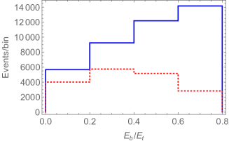
(a) Comparison of shapes of signal and background for LHC

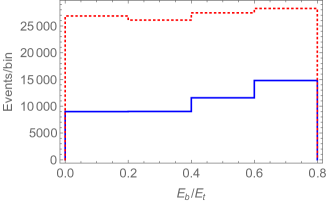
(b) Comparison of shapes of signal and background for FCC

Figure 3: Comparison of shapes of signal and background production cross-section for $1.5~{}\mathrm{TeV}$ left-handed leptoquark. The after-cut event analysis is done for 4 bins. Blue solid curve represents the $LQ$ signal and the red dotted curve represents the background. Different kinematic cuts (without MET cut) used to produce these plots as described in Section IV.

There are few interesting things to be noticed in this comparison of spectrum analysis for the LHC and the FCC collider. First, from the Table 2 we see that there is a significant increase of the pre-cut cross-section for LQ in the FCC analysis compared to the LHC case, it is almost $18000$ times larger, whereas the same for the $t\bar{t}$ is almost $40$ times only. Second, although the efficiency of the signal events remains the same for both LHC and FCC, that of the background increases largely for the FCC analysis. Third the final efficiency of getting the $b$-energy ratio for LQs are comparable in both cases. Fourth and most importantly, the plots show similar nature in both collider analysis and thus can be used to probe the chirality of the LQs in the collider analysis depending on the sensitivity.

V.2 MET cut analysis

We know that in collider, missing transverse energy comes from the particles which either do not or weakly interact with the electromagnetic and strong forces and thus escape the detection. Thus in collider physics it is an extremely important observable for discriminating leptonic decays of $W$ bosons and top quarks from background events such as multijet and Drell–Yan events, because they do not contain neutrinos. As we have considered specifically the hadronic decays with neutrino of our leptoquark, the MET analysis provide us very useful information about separating the signal events from the possible backgrounds. The basic idea is that, if there are neutrinos which are the decay product of the LQs, then they will contribute significantly towards generating a MET cut plot of significant slope and a clear signature of the presence of the leptoquarks as the parent particles.

Collider	LQ Energy cut Eff	LQ MET cut Eff	t$\bar{t}$ Energy cut Eff	t$\bar{t}$ MET cut Eff
LHC $(\sqrt{s}=13~{}~{}\mathrm{TeV})$	0.32	0.97	0.36	0.02
FCC $(\sqrt{s}=100~{}~{}\mathrm{TeV})$	0.36	0.98	0.34	0.02

Table 3: Cut-efficiency flow table for signal and background after MET cut at different colliders

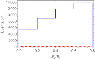
(a) MET cut $150~{}\mathrm{GeV}$ for LHC.

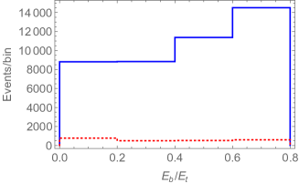
(b) MET cut $150~{}\mathrm{GeV}$ for FCC.

Figure 4: Comparison of signal and background events with MET cut $150~{}\mathrm{GeV}$ at the LHC and FCC

This clearly follows from the table as well as from the following figures. Table 3 shows although the energy cut efficiencies are comparable, the MET cut efficiency of the background is negligible compared to the signal. From Fig. 4(a) also we find that for LHC analysis putting a MET cut of $150~{}\mathrm{GeV}$ the backgrounds can be completely eliminated. If we compare this with Fig. 3(a) we see that a clear signature of left-handed LQ is obtained. Similar trend can also be observed for the FCC analysis. Since we have considered only the hadronic decay of the LQs we are ignoring the possible leptonic and semi-leptonic decays of the backgrounds, although it is quite possible that even we consider them they can not pass through the cuts applied and contribute significantly. It is interesting to notice that, although in FCC the background is higher than the LHC as we see from Fig 3, with the MET cut analysis we can get distinguish the $LQ$ signal from the background.

V.3 Sensitivity analysis

The whole analysis described above gave us two important informations. First, the shape of the LQ signal, with a definite chirality, curve compared to the dominant background and second, the efficiency with different kinematic cuts. We can use this cut-efficiency to find some numbers relevant for the collider study. We did two such estimations here. First is the estimation of number of events for different luminosities at different colliders and the second is the sensitivity test to find the luminosity required to get the $(\chi^{2})$ value with $95\%$ C.L. The results are given in Table 4.

To get the expected number of events at the LHC, we just used $N_{evts}=\sigma\times\rm BR\times\rm Efficiency\times\rm Luminosity(\mathscr{L})$ where $\sigma$ is the only production cross-section of the signal events at different center of mass energies, ($13~{}\mathrm{TeV}$) for LHC and ($100~{}\mathrm{TeV}$) for FCC-hh. Thus choosing the recent luminosity of $(150fb^{-1})$ used by the LHC, we find there is a possibility of getting only $1$ event whereas for the FCC-hh we can get a significantly higher number of signal events, as shown in the table, at the luminosity of $(1000fb^{-1})$ which is about half of the predicted luminosity for the first phase $(2500fb^{-1})$ of FCC-hh.

To perform a sensitivity test, means how much luminosity is required to get similar results as our analysis, for different colliders we wrote a chi-square $(\chi^{2})$ function which is a function of luminosity only, see Appendix A for details. That function is fed with the values of 4-bin analysis we got after putting all the cuts including energy and MET cut as described in Sec. IV. Finally we solve for the required luminosity against the number for $95\%$ C.L with four variables, since we used four bins for our analysis.

Collider	Number of Events $(N_{evts})$	Luminosity ($fb^{-1})$
LHC $(\sqrt{s}=13~{}~{}\mathrm{TeV})$	$1.5~{}(150fb^{-1})$	$3.64\times 10^{5}$
FCC-hh $(\sqrt{s}=100~{}~{}\mathrm{TeV})$	$2.2\times 10^{5}~{}(1000fb^{-1})$	$0.363$

Table 4: Sensitivity analysis for different colliders

VI Conclusion

Using a purely left-handed vector LQ which can only couple to the third generation of quark and lepton, we have shown that it can decay to a pure left-handed top quark which in turn decays to a more energetic bottom quark. Since top quarks decay before the hadronization, we can reconstruct its energy and form a model-independent variable, $b$-energy ratio which can be used as a clear distinguishable signature of tops chirality and consequently the chirality of the leptoquark of which top is the decay product.

In the FCC analysis the SM t$\bar{t}$ background is significantly higher but from the nature of the spectrum the LQ signals are distinguishable. Following Table 2 we see there is a significant increase of two-top system efficiency which may contribute to this high background for the FCC-hh case, though this might be a topic of future investigation. Further with the MET cut analysis we have seen that we can reduce the backgrounds significantly and have a clear signature of left-handed signature.

Following Table 4 It is clear that the present or future LHC run are not sensitive to such analysis and the probability of getting sufficient signal events is almost negligible compared to the future collider like FCC which is quite sensitive for such production.

Appendix A $\chi^{2}$ (chi-square) Analysis

The quantity known as chi-square ($\chi^{2}$) is defined as

$$\chi^{2}\equiv\frac{(x_{1}-\mu_{1})^{2}}{\sigma_{1}^{2}}+\frac{(x_{2}-\mu_{2})^{2}}{\sigma_{2}^{2}}+\dots+\frac{(x_{\nu}-\mu_{\nu})^{2}}{\sigma_{\nu}^{2}}$$ (A.1)

where $\nu$ is the no of independent variables, $x_{i}$s are the independent variables, $\mu_{i}$s are the mean of each variable and $\sigma_{i}^{2}$ are the variance of each variable.

For our purpose the $x_{i}$s are the theoretical prediction which ideally should include both the production cross-section $\times\mathrm{BR}$ for the leptoquark production, known as signal, and the corresponding background. Assuming the background is eliminated we consider only the signal for $x_{i}$s. Therefore explicitly,

$$x_{i}=\big{(}\sigma_{\rm Sig}+\sigma_{\rm Bkg}\big{)}\times(\mathscr{L})\times\textrm{Fraction of events}(N_{i})$$ (A.2)

with $N_{i}=\frac{\textrm{Number of events in each bin}}{\textrm{Total number of events after MET cut}}$ and

$$\sigma_{\rm Sig}=\sigma(pp>LQ\bar{LQ})\times\rm{BR}(LQ>t\nu\cdots)\times\rm{MET~{}Eff},$$ (A.3)

similar for the $\sigma_{\rm Bkg}$.

Similarly $\mu_{i}$s in this case are the SM background obtained from $t\bar{t}$ pair production and given by

$$\mu_{i}=\sigma_{\rm Bkg}\times\textrm{Luminosity}(\mathscr{L})\times\textrm{Fraction of events}(N_{i}).$$ (A.4)

Therefore using equations A.2 and A.4 the final $\chi^{2}$ expression for our analysis of 4 bins become

$$\chi^{2}_{4\rm bins}=\sum_{i=1,4}\frac{(x_{i}-\mu_{i})^{2}}{\sigma_{i}}$$ (A.5)

where $\sigma_{i}=x_{i}+\mu_{i}$.

References

- (1) J. C. Pati and A. Salam, Phys. Rev. D 10, 275 (1974) [Erratum-ibid. D 11, 703 (1975)]. H. Georgi and S. L. Glashow, Phys. Rev. Lett. 32, 438 (1974). H. Georgi, Particles and Fields, 1974 (APS/DPF Williamsburg), ed. C. E. Carlson (AIP, New York, 1975) p.575; H. Fritzsch and P. Minkowski, “Unified Interactions Of Leptons And Hadrons,” Annals Phys. 93, 193 (1975). R. Slansky, Phys. Rept. 79, 1 (1981).
- (2) J. Heeck, “Unbroken B – L symmetry,” Phys. Lett. B 739, 256 (2014),[arXiv:1408.6845 [hep-ph]] .
- (3) I. Doršner, S. Fajfer, A. Greljo, J. F. Kamenik and N. Košnik, “Physics of leptoquarks in precision experiments and at particle colliders,” Phys. Rept. 641, 1 (2016), arXiv:1603.04993 [hep-ph].
- (4) J. M. Arnold, B. Fornal and M. B. Wise, “Phenomenology of scalar leptoquarks,” Phys. Rev. D 88, 035009 (2013) [arXiv:1304.6119 [hep-ph]].
- (5) S. Fajfer and N. Kosnik, “Leptoquarks in FCNC charm decays,” PhysRevD.79.017502, [arXiv:0810.4858 [hep-ph]].
- (6) M. Leurer, “A Comprehensive study of leptoquark bounds,” PhysRevD.49.333, [arXiv:[hep-ph/9309266]].
- (7) S. Sahoo and R. Mohanta, “Scalar leptoquarks and the rare meson decays,” PhysRevD.91.094019, [arXiv:1501.05193 [hep-ph]].
- (8) S. Sahoo and R. Mohanta, “Lepton flavor violating B meson decays via a scalar leptoquark,” Phys. Rev. D 93, no. 11, 114001 (2016), [arXiv:1512.04657 [hep-ph]].
- (9) M. Bauer and M. Neubert, Minimal Leptoquark Explanation for the R , RK , and Anomalies, Phys. Rev.Lett. 116 (2016) 141802, [arXiv:1511.01900 [hep-ph]]. D. Das, C. Hati, G. Kumar and N. Mahajan, Towards a unified explanation of , and anomalies in a left-right model with leptoquarks, Phys. Rev. D94 (2016) 055034, [arXiv:1605.06313 [hep-ph]]. D. Bečirević, S. Fajfer, N. Košnik and O. Sumensari, Leptoquark model to explain the -physics anomalies, and , Phys. Rev. D94 (2016) 115021, [arXiv:1608.08501[hep-ph]]. S. Sahoo, R. Mohanta and A. K. Giri, Explaining the and anomalies with vector leptoquarks, Phys. Rev. D95 (2017) 035027, [arXiv:1609.04367[hep-ph]]. G. Hiller, D. Loose and K. Schönwald, Leptoquark Flavor Patterns & B Decay Anomalies, JHEP 12 (2016) 027, [arXiv:1609.08895[hep-ph]]. B. Bhattacharya, A. Datta, J.-P. Guévin, D. London and R. Watanabe, Simultaneous Explanation of the and Puzzles: a Model Analysis, JHEP 01 (2017) 015, [arXiv:1609.09078[hep-ph]]. A. Crivellin, D. Müller and T. Ota, “Simultaneous explanation of R(D(∗)) and b→sμ+ μ−: the last scalar leptoquarks standing,” JHEP 1709, 040 (2017), [arXiv:1703.09226 [hep-ph]]. D. Bečirević and O. Sumensari, A leptoquark model to accommodate and , [arXiv:1704.05835[hep-ph]]. Y. Cai, J. Gargalionis, M. A. Schmidt and R. R. Volkas, Reconsidering the One Leptoquark solution: flavor anomalies and neutrino mass, [arXiv:1704.05849[hep-ph]]. D. Das, C. Hati, G. Kumar and N. Mahajan, Scrutinizing -parity violating interactions in light of data, [arXiv:1705.09188[hep-ph]]. N. Assad, B. Fornal and B. Grinstein, “Baryon Number and Lepton Universality Violation in Leptoquark and Diquark Models,” [Phys. Lett. B 777, 324 (2018) [arXiv:1708.06350 [hep-ph]]. M. Blanke and A. Crivellin, “ Meson Anomalies in a Pati-Salam Model within the Randall-Sundrum Background,” [Phys. Rev. Lett. 121, no. 1, 011801 (2018) [arXiv:1801.07256 [hep-ph]].
- (10) J. P. Lees et al. [BaBar Collaboration], Phys. Rev. D 88, no. 7, 072012 (2013), arXiv:1303.0571 [hep-ex].
- (11) R. Aaij et al. [LHCb Collaboration], Phys. Rev. Lett. 115, no. 11, 111803 (2015) Erratum: [Phys. Rev. Lett. 115, no. 15, 159901 (2015)] arXiv:1506.08614 [hep-ex].
- (12) A. Abdesselam et al. [Belle Collaboration], arXiv:1603.06711 [hep-ex].
- (13) R. Aaij et al. [LHCb Collaboration], Phys. Rev. D 97, no. 7, 072013 (2018), [[arXiv:1711.02505 [hep-ex]]]
- (14) S. Fajfer and N. Košnik, j.physletb.2016.02.018, arXiv:1511.06024 [hep-ph].
- (15) L. Calibbi, A. Crivellin and T. Ota, Phys. Rev. Lett. 115, 181801 (2015),arXiv:1506.02661 [hep-ph].
- (16) S. Sahoo, R. Mohanta and A. K. Giri, “Explaining the and anomalies with vector leptoquarks,” Phys. Rev. D 95, no. 3, 035027 (2017), [arXiv:1609.04367 [hep-ph]].
- (17) R. Allahverdi et al., “Distinguishing Standard Model Extensions using Monotop Chirality at the LHC,” JHEP 1612, 046 (2016), [arXiv:1507.02271 [hep-ph]].
- (18) L. Calibbi, A. Crivellin and T. Li, “A model of vector leptoquarks in view of the -physics anomalies,” Phys. Rev. D 98, no. 11, 115002 (2018),arXiv:1709.00692 [hep-ph].
- (19) A. K. Alok, B. Bhattacharya, A. Datta, D. Kumar, J. Kumar and D. London, “New Physics in after the Measurement of ,” Phys. Rev. D 96, no. 9, 095009 (2017), [arXiv:1704.07397 [hep-ph]].
- (20) D. Buttazzo, A. Greljo, G. Isidori and D. Marzocca, “B-physics anomalies: a guide to combined explanations,” JHEP 1711, 044 (2017), [arXiv:1706.07808 [hep-ph]]
- (21) A. Angelescu, D. Bečirević, D. A. Faroughy and O. Sumensari, “Closing the window on single leptoquark solutions to the -physics anomalies,” JHEP 1810, 183 (2018),[arXiv:1808.08179 [hep-ph]]
- (22) T. G. Rizzo, “Searches for scalar and vector leptoquarks at future hadron colliders,” eConf C 960625, NEW151 (1996) arxiv:9609267[hep-ph].
- (23) N. Vignaroli, “Seeking LQs in the plus missing energy channel at the high-luminosity LHC,” arXiv:1808.10309 [hep-ph].
- (24) A. Belyaev, C. Leroy, R. Mehdiyev and A. Pukhov, “Leptoquark single and pair production at LHC with CalcHEP/CompHEP in the complete model,” JHEP 0509, 005 (2005) Phys. Rev. D 96, no. 9, 095009 (2017),[arXiv:[hep-ph/0502067]].
- (25) N. D. Christensen and C. Duhr, “FeynRules - Feynman rules made easy,” Comput. Phys. Commun. 180, 1614 (2009), [arXiv:0806.4194 [hep-ph]].
- (26) A. M. Sirunyan et al. [CMS Collaboration], “Constraints on models of scalar and vector leptoquarks decaying to a quark and a neutrino at 13 TeV,” PhysRevD.98.032005 [arXiv:1805.10228 [hep-ex]].
- (27) C. Degrande, C. Duhr, B. Fuks, D. Grellscheid, O. Mattelaer and T. Reiter, “UFO - The Universal FeynRules Output,” Comput. Phys. Commun. 183, 1201 (2012), [arXiv: [arXiv:1108.2040 [hep-ph]].
- (28) J. Alwall et al., “The automated computation of tree-level and next-to-leading order differential cross sections, and their matching to parton shower simulations,” JHEP 1407, 079 (2014), [arXiv:1405.0301 [hep-ph]].
- (29) T. Sjöstrand et al., “An Introduction to PYTHIA 8.2,” Comput. Phys. Commun. 191, 159 (2015),[arXiv:1410.3012 [hep-ph]].
- (30) J. de Favereau et al. [DELPHES 3 Collaboration], “DELPHES 3, A modular framework for fast simulation of a generic collider experiment,” JHEP 1402, 057 (2014), [arXiv:1307.6346 [hep-ex]].
- (31) V. Khachatryan et al. [CMS Collaboration], Phys. Rev. Lett. 116, no. 5, 052002 (2016) PhysRevLett.116.052002, arXiv:1510.05302 [hep-ex].
- (32) Future Circular Collider Study Kickoff Meeting.
- (33) F. Su, J. Gao, M. Xiao, D. Wang, Y. W. Wang, S. Bai and T. J. Bian, “Method study of parameter choice for a circular proton–proton collider,” Chin. Phys. C 40, no. 1, 017001 (2016), arXiv:1503.01530 [physics.acc-ph].