Early-time dynamics of Bose gases quenched into the strongly interacting regime

Abstract

We study the early-time dynamics of a degenerate Bose gas after a sudden quench of the interaction strength, starting from a weakly interacting gas. By making use of a time-dependent generalization of the Nozières-Saint-James variational formalism, we describe the crossover of the early-time dynamics from shallow to deep interaction quenches. We analyze the coherent oscillations that characterize both the density of excited states and the Tan’s contact as a function of the final scattering length. For shallow quenches, the oscillatory behaviour is negligible and the dynamics is universally governed by the healing length and the mean-field interaction energy. By increasing the final scattering length to intermediate values, we reveal a universal regime where the period of the coherent atom-molecule oscillations is set by the molecule binding energy. For the largest scattering lengths we can numerically simulate in the unitary regime, we find a universal scaling behaviour of the typical growth time of the momentum distribution in agreement with recent experimental observations [C. Eigen et al., Nature 563, 221 (2018)].

I Introduction

The possibility of tuning the effective interatomic interaction in ultracold atomic gases via a magnetic-field Feshbach resonance Chin et al. (2010) opens up novel perspectives in the exploration of quantum many-body phenomena and strongly correlated behavior. In particular, it is now possible to experimentally investigate strongly interacting Bose gases near the unitary limit, where the $s$-wave scattering length diverges, $a\to\infty$ Fletcher et al. (2013); Rem et al. (2013); Makotyn et al. (2014); Eismann et al. (2016); Klauss et al. (2017); Lopes et al. (2017); Fletcher et al. (2017); Eigen et al. (2017, 2018). Such a system is inherently unstable due to strong three-body losses to lower lying states, and thus experiments must access the strongly interacting regime by starting with a weakly interacting Bose gas and then rapidly ramping the external magnetic field to the desired scattering length. However, rather than being a complication, this provides a unique opportunity to study the dynamics of a quantum many-body system driven out of equilibrium in a controlled manner. For instance, for shallow quenches within the weakly interacting regime, it has been possible to reconstruct the spectrum of collective excitations of the degenerate gas from the characteristic oscillations of the density-density correlation function Hung et al. (2013), which is the analogue of cosmological Sakharov oscillations.

For the case of deep quenches into the unitary regime, there are fundamental questions regarding the role and nature of three-body losses in the evolution of the Bose gas Fletcher et al. (2013); Rem et al. (2013); Klauss et al. (2017); Eismann et al. (2016); Eigen et al. (2017). A pioneering experiment Makotyn et al. (2014) has shown that the momentum distribution of a degenerate gas can saturate to a prethermal steady-state distribution, thus suggesting that the early-time dynamics after a deep quench is unaffected by three-body recombination. Most recently, C. Eigen et al. Eigen et al. (2018) have observed a universal prethermal post-quench dynamics of the degenerate gas at unitarity. Here, the authors have found scaling laws of the momentum-distribution growth time versus momentum, which are universal when expressed in terms of density scales. These results indicate that, in the post-quench dynamics at very short times, the quasi-particle excitations of the unitary gas are qualitatively similar to the Bogoliubov modes. As we show in this paper, this behaviour can be described without including three-body scattering or losses.

The observed universal dynamics of the unitary Bose gas is consistent with the scale invariance one expects when the scattering length diverges and there is no interaction scale in the problem. This would appear to contradict the existence of Efimov trimers Efimov (1970), which introduces another length scale in the problem and thus breaks the scale invariance of the degenerate Bose gas Braaten and Hammer (2006). However, experiments on the thermal gas Fletcher et al. (2017) have shown that the three-body contact $C_{3}$ Smith et al. (2014) (which provides a measure of the three-body correlations connected with Efimov trimers) is negligible in an early time window after a quench into the unitary regime. Therefore, this suggests that Efimov physics is only important at later times in the dynamics, which is reasonable given that we expect short times to be dominated by short-distance, two-body scattering. Furthermore, the typical density range in many experiments may be insensitive to the Efimov scale Eigen et al. (2017).

In general, the quench dynamics of Bose gases near unitarity is a challenge to describe theoretically Yin and Radzihovsky (2013); Sykes et al. (2014); Rançon and Levin (2014); Kain and Ling (2014); Corson and Bohn (2015); Kira (2015); Ancilotto et al. (2015); Yin and Radzihovsky (2016) since there is no small interaction parameter that allows a perturbative expansion. However, in the early stages of the dynamics after a quench from weak interactions, we expect three-body correlations and losses to be negligible, as discussed above. Therefore, a theory involving only pairwise excitations out of the condensate should be reasonable at short times. To this end, we employ here a time-dependent generalization of the Nozières-Saint James variational formalism Nozières, P. and Saint James, D. (1982), similarly to the approach in Refs. Sykes et al. (2014); Corson and Bohn (2015). This also allows us to capture the effect of the molecular two-body bound state, which is present on the repulsive side of the resonance, $a>0$.

We go beyond previous work and analyze the crossover from shallow to deep quenches using the variational formalism. For shallow quenches the early-time dynamics is integrable Natu and Mueller (2013); Hung et al. (2013); Van Regemortel et al. (2018) and one can make use of a time-dependent Bogoliubov approximation. However, in order to describe the crossover to deep quenches, we have to resort to a numerical analysis of the coupled dynamical equations for the condensate density and the excited state distribution, which, in our modelling, includes the condensate depletion as well as the correlations between non-condensed atoms.

We describe the coherent oscillations developed by the number of excited particles as well as by the Tan’s contact and, up to intermediate values of the final scattering length $a_{f}$, we disclose a universal regime where the oscillation period is constant and determined by the inverse molecule binding energy only. We discuss the optimal values of $a_{f}$ at which these atom-molecule coherent oscillations should be detectable in current experiments.

For the largest scattering lengths we can numerically simulate in the unitary regime, we find that the coherent oscillations persist and are now due to the condensate interaction with the medium. While these oscillations appear strongly damped in current experiments Eigen et al. (2018), our model can correctly reproduce the universal scaling behaviour of the typical growth time of the momentum distribution found by Ref. Eigen et al. (2018), suggesting that higher-order damping mechanisms do not affect the postquench behaviour at very-early times, when a steady state regime is not yet reached.

The paper is organized as follows: In Sec. II we introduce the variational Ansatz for describing the quench dynamics and, in Sec. II.1, we derive the coupled equations of motion for the condensate density and excited state distribution. We summarize in Sec.  II.2 the characteristic system parameters as well as the relevant length and time scales in the crossover from shallow to deep quenches. In Sec. III, we present the numerical results for the non-condensed fraction (Sec. III.1) and the Tan’s contact (Sec. III.2), while in Sec. III.3 we explore the universal scaling laws associated with the very-early-time dynamics of the gas momentum distribution in the unitary regime. Conclusions and perspectives of our work are summarized in Sec. IV.

II Model

We start by considering the Hamiltonian describing a homogeneous gas of $N$ interacting bosons in a three-dimensional (3D) volume $V$ (henceforth we fix $\hbar=1$)

$$\hat{H}=\sum_{\mathbf{k}}\epsilon_{\mathbf{k}}\hat{a}_{{\mathbf{k}}}^{\dagger}\hat{a}_{{\mathbf{k}}}+\frac{U_{\Lambda}}{2V}\sum_{\mathbf{k}_{1},\mathbf{k}_{2},\mathbf{q}}\hat{a}_{\mathbf{k}_{1}+\mathbf{q}}^{\dagger}\hat{a}_{\mathbf{k}_{2}-\mathbf{q}}^{\dagger}\hat{a}_{\mathbf{k}_{2}}\hat{a}_{\mathbf{k}_{1}}\;,$$ (1)

where $\hat{a}_{\mathbf{k}}^{\dagger}$ ($\hat{a}_{\mathbf{k}}$) creates (annihilates) a boson with momentum $\mathbf{k}$ and mass $m$ ($\epsilon_{\mathbf{k}}=|\mathbf{k}|^{2}/2m\equiv k^{2}/2m$). Close to a Feshbach resonance, atom-atom interactions can be modelled via a short-range pseudo-potential, which, in momentum space, is constant with strength $U_{\Lambda}$ up to a momentum cutoff $\Lambda$. The coupling constant and cutoff are related to the $s$-wave scattering length $a$ through the $T$-matrix renormalization process Chin et al. (2010); Gurarie and Radzihovsky (2007):

$$\frac{m}{4\pi a}=\frac{1}{U_{\Lambda}}+\frac{1}{V}\sum_{\mathbf{k}}^{k<\Lambda}\frac{1}{2\epsilon_{\mathbf{k}}}=\frac{1}{U_{\Lambda}}+\frac{m\Lambda}{2\pi^{2}}\;.$$ (2)

The (inverse) cutoff $\Lambda^{-1}$ represents the range of the interaction potential, which is assumed to be much smaller than all other length scales in the problem. In the limit $\Lambda\to\infty$, the contact potential admits, on the repulsive side of the resonance $a>0$, a single molecular bound state with energy Gurarie and Radzihovsky (2007):

$$E_{\text{B}}=-\displaystyle\frac{1}{ma^{2}}\;.$$ (3)

We have checked that our results are converged with respect to the cutoff $\Lambda$.

In order to separate the contribution of the condensed state ${\mathbf{k}}={\mathbf{0}}$ from that of the excited states ${\mathbf{k}}\neq{\mathbf{0}}$, it is useful to rewrite the Hamiltonian (1) by substituting $\hat{a}_{\mathbf{k}}\rightarrow\hat{a}_{0}\delta_{\mathbf{k}\,,{\mathbf{0}}}+\hat{a}_{\mathbf{k}\neq{\mathbf{0}}}$. One thus obtains the following contributions to the Hamiltonian (we henceforth use the notation $\hat{a}_{\mathbf{k}}$ for $\hat{a}_{\mathbf{k}\neq{\mathbf{0}}}$):

$$\hat{H} =\sum_{\mathbf{k}}\epsilon_{\mathbf{k}}\hat{a}_{{\mathbf{k}}}^{\dagger}\hat{a}_{{\mathbf{k}}}+\frac{U_{\Lambda}}{2V}\hat{a}_{0}^{\dagger}\hat{a}_{0}^{\dagger}\hat{a}_{0}\hat{a}_{0}+\hat{H}_{2}+\hat{H}_{3}+\hat{H}_{4}$$ (4)

$$\hat{H}_{2} =\frac{U_{\Lambda}}{2V}\sum_{\mathbf{k}}\left(\hat{a}_{\mathbf{k}}^{\dagger}\hat{a}_{-\mathbf{k}}^{\dagger}\hat{a}_{0}\hat{a}_{0}+2\hat{a}_{\mathbf{k}}^{\dagger}\hat{a}_{\mathbf{k}}\hat{a}_{0}^{\dagger}\hat{a}_{0}+\text{h.c.}\right)$$ (5)

$$\hat{H}_{3} =\frac{U_{\Lambda}}{V}\sum_{\mathbf{k},\mathbf{q}}\left(\hat{a}_{\mathbf{k}-\mathbf{q}}^{\dagger}\hat{a}_{\mathbf{q}}^{\dagger}\hat{a}_{\mathbf{k}}\hat{a}_{0}+\text{h.c.}\right)$$ (6)

$$\hat{H}_{4} =\frac{U_{\Lambda}}{2V}\sum_{\mathbf{k}_{1},\mathbf{k}_{2},\mathbf{q}}\hat{a}_{\mathbf{k}_{1}+\mathbf{q}}^{\dagger}\hat{a}_{\mathbf{k}_{2}-\mathbf{q}}^{\dagger}\hat{a}_{\mathbf{k}_{2}}\hat{a}_{\mathbf{k}_{1}}\;.$$ (7)

In the following, we focus on zero temperature and consider the early-time dynamics of the gas after a quench from an initial scattering length $a_{i}$ to the final value $a_{f}$. We will not carry out any approximation at the level of the Hamiltonian (4), unlike what is done in the time-dependent self-consistent Bogoliubov approximation Yin and Radzihovsky (2016). Instead, we will use the time-dependent generalization of the Nozières-Saint-James variational Ansatz Nozières, P. and Saint James, D. (1982); Song and Zhou (2009):

$$\ket{\psi(t)}=\frac{1}{\mathcal{N}(t)}e^{\sqrt{V}c_{0}(t)\hat{a}^{\dagger}_{0}+\frac{1}{2}\operatorname*{\bar{\sum}}_{\mathbf{k}}g_{\mathbf{k}}(t)\hat{a}^{\dagger}_{\mathbf{k}}\hat{a}^{\dagger}_{-\mathbf{k}}}\ket{0}\;.$$ (8)

Here, the normalization constant $\mathcal{N}(t)$ ensures that $\bra{\psi(t)}\ket{\psi(t)}=1$. The complex variational parameters $c_{0}(t)$ and $g_{\mathbf{k}}(t)$ are related to the momentum occupation numbers,

$$N_{0}(t) =|\langle\hat{a}_{0}\rangle|^{2}=V|c_{0}(t)|^{2}$$ (9)

$$N_{\mathbf{k}}(t) =\langle\hat{a}^{\dagger}_{\mathbf{k}}\hat{a}_{\mathbf{k}}\rangle=\frac{|g_{\mathbf{k}}(t)|^{2}}{1-|g_{\mathbf{k}}(t)|^{2}}\;,$$ (10)

as well as to the pairing term:

$$x_{\mathbf{k}}(t)=\langle\hat{a}_{\mathbf{k}}\hat{a}_{-\mathbf{k}}\rangle=\frac{g_{\mathbf{k}}(t)}{1-|g_{\mathbf{k}}(t)|^{2}}\;,$$ (11)

where $\langle\dots\rangle=\bra{\psi(t)}\dots\ket{\psi(t)}$. Note that $N_{\mathbf{k}}(t)$ and $x_{\mathbf{k}}(t)$ are not independent functions, since they are related by the constraint $|x_{\mathbf{k}}(t)|^{2}=N_{\mathbf{k}}(t)\left[N_{\mathbf{k}}(t)+1\right]$. Also note that $g_{-\mathbf{k}}(t)=g_{\mathbf{k}}(t)$, while the factor $1/2$ in the momentum sum in Eq. (8) avoids double-counting. We use the notation $\operatorname*{\bar{\sum}}_{\mathbf{k}}=\sum^{k<\Lambda}_{\mathbf{k}\neq{\mathbf{0}}}$.

The Ansatz $\ket{\psi(t)}$ describes the $\mathbf{k}=\mathbf{0}$ condensed state as a coherent state, while particles at finite momentum $\mathbf{k}\neq\mathbf{0}$ are excited out of the condensate in pairs only. For shallow quenches ($na_{i,f}^{3}\ll 1$), the condensate depletion is small, such that one can assume that the condensate density is time independent, $|c_{0}(t)|^{2}\simeq n$. In this case, the Ansatz (8) is a controlled approximation at an early stage of the dynamics, where Beliaev-Landau scattering processes involving three particles can be safely neglected Van Regemortel et al. (2018). Here, one can neglect the contributions of $\hat{H}_{3}$ and $\hat{H}_{4}$ to the Hamiltonian (4) and show that the dynamics becomes integrable (see App. A), which recovers the results obtained by Refs. Natu and Mueller (2013); Hung et al. (2013) within a time-dependent Bogoliubov approximation.

The same Ansatz (8) has previously been employed by Refs. Sykes et al. (2014); Corson and Bohn (2015) to describe the quench dynamics of a Bose gas into the strongly interacting regime. Assuming a weakly interacting initial state ($na_{i}^{3}\ll 1$), we will use the Ansatz (8) to study the crossover of the early-time dynamics from shallow to deep quenches, where $na_{f}^{3}\ll 1$ and $na_{f}^{3}\gtrsim 1$, respectively. In general, the dynamics of the condensate depletion cannot be neglected and we include the time dependence of the variational parameter $c_{0}(t)$ in a similar way to the self-consistent Bogoliubov approximation considered by Ref. Yin and Radzihovsky (2016). Further, as explained later, we include all contributions arising from $\langle\hat{H}_{4}\rangle$ which describes the correlations between non-condensed atoms. This, together with the renormalization of the interaction coupling constant (2), allows one to describe the atom-molecule coherent dynamics, as already discussed in Ref. Corson and Bohn (2015). However, as $\langle\hat{H}_{3}\rangle=0$, the Ansatz for $\ket{\psi(t)}$ does not admit neither Beliaev decay nor Landau damping terms that may be responsible for the loss of the atom-molecule coherence.

For weak interactions, Ref. Van Regemortel et al. (2018) has shown that there is a separation of time scales between short-time dynamics dominated by pair-wise excitations and longer-time dynamics requiring the inclusion of higher-order excitation terms such as $\hat{H}_{3}$. However, it remains an open question how this separation of time scales evolves as we approach unitarity. For the case of an impurity atom immersed in a quantum medium, it can be formally shown that the dynamics following a quench of the impurity-medium interactions to the unitary regime is dominated by two-body correlations at times less than the time scale $\epsilon_{n}^{-1}$ set by the density Parish and Levinsen (2016). Moreover, recent experiments on the very-early-time dynamics of quantum quenches in the Bose gas Eigen et al. (2018) suggest that a similar situation holds for the unitary Bose gas. To investigate this further, one must generalize Eq. (8) to include three-particle processes, but this is beyond the scope of this work and will be the subject of future studies.

II.1 Equations of motion

As in Refs. Sykes et al. (2014); Corson and Bohn (2015), the equations of motion for the variational parameters $c_{0}(t)$ and $g_{\mathbf{k}}(t)$ can be derived from the Euler-Lagrange equations Kramer (2008); Corson and Bohn (2015),

$$\frac{d}{dt}\frac{\partial\mathcal{L}}{\partial\dot{c}^{*}_{0}} =\frac{\partial\mathcal{L}}{\partial c^{*}_{0}} \frac{d}{dt}\frac{\delta\mathcal{L}}{\delta\dot{g}^{*}_{\mathbf{k}}} =\frac{\delta\mathcal{L}}{\delta g^{*}_{\mathbf{k}}}\;,$$

associated with the Lagrangian

$$\mathcal{L}=\frac{i}{2}\left[\langle\psi(t)|\dot{\psi}(t)\rangle-\langle\dot{\psi}(t)|\psi(t)\rangle\right]-\langle\hat{H}\rangle\;.$$

When evaluating the contributions to $\langle\hat{H}\rangle$, we have that $\langle\hat{H}_{3}\rangle$ = 0 while

$$\expectationvalue*{\hat{H}_{4}}=\frac{U_{\Lambda}}{2V}\operatorname*{\bar{\sum}}_{{\mathbf{k}},{\mathbf{q}}}\left[2N_{\mathbf{k}}(t)N_{\mathbf{q}}(t)+x_{\mathbf{k}}(t)x^{*}_{\mathbf{q}}(t)\right]\;.$$ (12)

Differently from Yin and Radzihovsky (2016); Kain and Ling (2014), we retain the anomalous expectation values $x_{\mathbf{k}}$ in $\expectationvalue*{\hat{H}_{4}}$. One arrives at the following equations of motion:

$$i\dot{c}_{0} =U_{\Lambda}c_{0}n+\frac{U_{\Lambda}}{V}\operatorname*{\bar{\sum}}_{\mathbf{k}}\frac{c_{0}|g_{\mathbf{k}}|^{2}+c^{*}_{0}g_{\mathbf{k}}}{1-|g_{\mathbf{k}}|^{2}}$$ (13)

$$i\dot{g}_{\mathbf{k}} =2\left[\epsilon_{\mathbf{k}}+U_{\Lambda}n\right]g_{\mathbf{k}}+U_{\Lambda}\big{(}2|c_{0}|^{2}g_{\mathbf{k}}+g_{\mathbf{k}}^{2}c^{*2}_{0}$$

$$+c^{2}_{0}\big{)}+\frac{U_{\Lambda}}{V}\operatorname*{\bar{\sum}}_{\mathbf{q}}\frac{2g_{\mathbf{k}}|g_{\mathbf{q}}|^{2}+g^{2}_{\mathbf{k}}g^{*}_{\mathbf{q}}+g_{\mathbf{q}}}{1-|g_{\mathbf{q}}|^{2}}\;,$$ (14)

that have to be solved for a set of initial conditions $c_{0}(0)$ and $g_{\mathbf{k}}(0)$. Note that the total density

$$n=n_{0}(t)+n_{ex}(t)=|c_{0}(t)|^{2}+\displaystyle\frac{1}{V}\operatorname*{\bar{\sum}}_{{\mathbf{k}}}N_{{\mathbf{k}}}(t)\;,$$ (15)

is conserved during the dynamics governed by Eqs. (13) and (14).

For instantaneous quenches $a_{i}\mapsto a_{f}$, the system is initially ($t=0$) characterized by the scattering length $a_{i}$, while at later times $t>0$ it evolves with the interaction set by the final scattering length $a_{f}$. Therefore, the equations of motion (13) and (14) have to be solved by using $U_{\Lambda}=U_{\Lambda,f}=(1-2a_{f}\Lambda/\pi)^{-1}4\pi a_{f}/m$. The initial state is assumed to be in equilibrium and thus can be found by minimizing $\bra{\psi}\hat{H}-\mu\hat{N}\ket{\psi}$ with respect to time-independent variational parameters $c_{0}(0)$ and $g_{\mathbf{k}}(0)$, where $U_{\Lambda}=U_{\Lambda,i}$ and the Lagrange multiplier $\mu$ (i.e., the chemical potential) fixes the number of particles. For example, for an initial weakly interacting gas $na_{i}^{3}\ll 1$, one has that

$$|c_{0}(0)|^{2} =n\left(1-\displaystyle\frac{8}{3\sqrt{\pi}}\sqrt{na_{i}^{3}}\right)\simeq n$$ (16)

$$g_{{\mathbf{k}}}(0) =\displaystyle\frac{\sqrt{\epsilon_{{\mathbf{k}}}(\epsilon_{{\mathbf{k}}}+2U_{i}n)}-(\epsilon_{{\mathbf{k}}}+nU_{i})}{nU_{i}}\;,$$ (17)

where $U_{i}=4\pi a_{i}/m$.

The last two terms in the equation for the condensate dynamics (13) self-consistently describe the condensate depletion due to the scattering to finite momentum excited states. The last three terms in the equation for the excited state dynamics (14) instead represent the correlations between non-condensed atoms. As shown in App. A, for shallow quenches $na_{i,f}^{3}\ll 1$, the dynamics is integrable, the terms just described can be neglected, and the now simplified Eqs. (25) and (26) can be solved exactly. However, for a generic quench from a weakly interacting gas $na_{i}^{3}\ll 1$ to an arbitrary value of the final scattering length $a_{f}$, the dynamics is not integrable and one has to carry out a numerical analysis.

$a$	$ak_{n}$	$\xi$	$\tau$	$|E_{B}|^{-1}$	$k_{n}^{-1}$	$\epsilon_{n}^{-1}$
$100a_{0}$	$2.1\times 10^{-2}$	$3$ $\mu$m	$9$ ms	$20$ ns	$0.3$ $\mu$m	$80~{}\mu$s
$1000a_{0}$	$2.1\times 10^{-1}$	$0.9$ $\mu$m	$0.9$ ms	$2$ $\mu$s	$0.3$ $\mu$m	$80~{}\mu$s
$60000a_{0}$	$12$	$0.1$ $\mu$m	$15$ $\mu$s	$6$ ms	$0.3$ $\mu$m	$80~{}\mu$s

Table 1: Dimensionless interaction strength $ak_{n}$ in units of $k_{n}=(6\pi^{2}n)^{1/3}$ and characteristic length and time scales for different values of scattering length $a$ (in units of the Bohr radius $a_{0}$) for a ³⁹K gas with density $n=10^{12}$ cm^-3. We indicate in grey all those scales that we expect to be irrelevant in a specific regime. The value $a=60000a_{0}$ is the largest final scattering length we can numerically simulate.

II.2 System parameters

Before describing the results obtained from the numerical simulations, we summarize here the system characteristic length and time scales that we expect to be relevant for different values of the final scattering length $a_{f}$. For shallow quenches $na_{i,f}^{3}\ll 1$, the early-time quasiparticle dynamics can be derived by using the time-dependent Bogoliubov approximation Natu and Mueller (2013); Hung et al. (2013) and can thus be described is terms of the healing length and mean-field time scales only Pitaevskii and Stringari (2003):

$$\xi =\displaystyle\frac{1}{\sqrt{8\pi an}} \tau =\displaystyle\frac{m}{4\pi an}\;.$$ (18)

In fact, it can be shown that, in this regime, the dynamics is universal in terms of these two parameters, where $a$ is taken to be the final scattering length $a_{f}$. Here, the Bose gas occupies the metastable upper branch at positive energies, and the molecular bound state is far below the continuum when $na_{f}^{3}\ll 1$. As shown later on, while atom-molecule coherent oscillations occur on a time scale $|E_{\text{B}}|^{-1}\ll\tau$ (see Tab. 1), their amplitude is negligible in this limit since they rescale as $na_{f}^{3}\ll 1$.

Increasing the value of the final scattering length $a_{f}$ beyond the weakly interacting regime, we anticipate that all scales play a role in the description of the dynamics — typical values for a ³⁹K gas with density $n=10^{12}$ cm^-3 are listed in Tab. 1. However, in the unitary regime $a_{f}\to\infty$, we expect the dynamics to recover a universal behaviour in terms of the density scales only, i.e., in terms of the typical momentum and energy scales:

$$k_{n} =(6\pi^{2}n)^{1/3} \epsilon_{n} =\displaystyle\frac{k_{n}^{2}}{2m}\;.$$ (19)

In particular, we will see that, in the unitary regime, the typical growth time $\tau_{gr}$ of the number of excited particles in a given momentum state ${\mathbf{k}}$ follows a universal scaling law when rescaled by $\epsilon_{n}^{-1}$ and $k_{n}$, respectively. Here, all other system scales become irrelevant in the very-early-time quench dynamics of the gas.

Of course, the arguments above ignore the existence of Efimov trimers, which introduce an additional length scale in the problem. Therefore, one might wonder about the typical time scales at which three-body correlations and losses become relevant in the quench dynamics. It was found in Ref. Fletcher et al. (2017) that for a thermal Bose gas of ³⁹K atoms trapped in a harmonic potential and quenched to large values of the scattering length ($na_{f}^{3}\gg 1$), the three-body contact $C_{3}$ was negligible in the early stages of the dynamics where $t\lesssim 5\epsilon_{n}^{-1}$ — note that the density in this experiment was $n\simeq 2.8\times 10^{13}$ cm^-3, so that $\epsilon_{n}^{-1}\approx 9$ $\mu$s. More recently, it was shown in Ref. Eigen et al. (2018) that, for a box potential trap, interaction quenches to the unitary regime for a degenerate ³⁹K gas have a universal dynamics and are lossless up to $t\simeq\epsilon_{n}^{-1}$ — in that experiment a density of $n=5.1\times 10^{12}$ cm^-3 was considered, and thus $\epsilon_{n}^{-1}\simeq 27~{}\mu$s, while in the Tab. 1 we have fixed $n=10^{12}$ cm^-3 and thus $\epsilon_{n}^{-1}\simeq 80~{}\mu$s.

III Results

We describe here how the early-time quench dynamics of a Bose condensate at zero temperature evolves as a function of the final scattering length $a_{f}$ all the way towards unitarity. To this end, we numerically solve the equations of motion (13) and (14) for the specific case of instantaneous quenches from a non-interacting gas ($a_{i}=0$, $c_{0}(0)=\sqrt{n}$ and $g_{{\mathbf{k}}}(0)=0$) to a generic value $a_{f}$. Since we are considering $s$-wave interactions, we can assume spherical symmetry for the function $g_{\mathbf{k}}(t)=g_{k}(t)$. We use a Gauss-Legendre quadrature routine on a grid of $M$ points in $k$-space and integrate the equations of motion using a 5${}^{\text{th}}$-order Runge-Kutta routine. We have checked our results are converged with respect to the chosen time step. The dynamics has therefore two regularization parameters, namely the number of points $M$ on the Gauss-Legendre momentum grid and the momentum cutoff $\Lambda$. As explained in App. B, we have checked the convergence of our results with respect to both parameters and extrapolated the results from the numerics to both $M\to\infty$ and $\Lambda\to\infty$ limits. Note that, in the limit $\Lambda\to\infty$, our results do not depend on the density $n$ and the final scattering length $a_{f}$ separately; rather they depend on the dimensionless interaction strength $a_{f}k_{n}$.

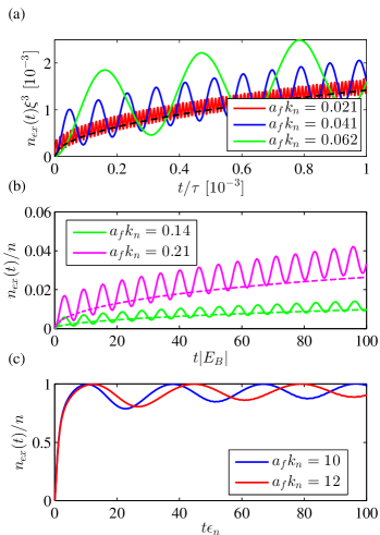
Figure 1: Non-condensed density $n_{ex}(t)$ as a function of time after an instantaneous quench from a non-interacting gas $a_{i}=0$ to different values of the final scattering length $a_{f}$. In all panels, solid lines are the results of the numerical integration of the equations of motion (13) and (14). (a) For shallow quenches, density and time are rescaled by the healing length $\xi$ and mean-field time $\tau$ (18), respectively. At intermediate values of $a_{f}$ (b), it is convenient to rescale the time by the molecular molecular bound state energy $|E_{\text{B}}|$, while, towards unitarity (c), by the energy scale fixed by the gas density $\epsilon_{n}$. In panels (a) and (b), the dashed lines are obtained via the time-dependent Bogoliubov approximation Natu and Mueller (2013) (see Eq. (31)).

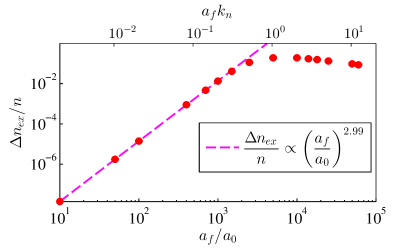
Figure 2: Amplitude of coherent oscillations for the non-condensed fraction $\Delta n_{ex}$ as a function of $a_{f}k_{n}$ ($a_{f}$ in units of the Bohr radius $a_{0}$ is given for a density $n=10^{12}$ cm^-3).

III.1 Non-condensed fraction

We plot in Fig. 1 the density of particles in the excited states $n_{ex}(t)$ (15) as a function of time after an instantaneous quench from the non-interacting case $a_{i}=0$, and for different values of the final scattering length $a_{f}$. It is convenient to rescale both the non-condensed density $n_{ex}(t)$ and the time $t$ by different scales depending on the different range of final scattering lengths $a_{f}$ considered. In the weakly interacting regime (panel (a)), we rescale density and time using the healing length $\xi$ and mean-field time $\tau$ (18), respectively. In this regime, the dynamics obtained within the time-dependent Bogoliubov approximation ([black] dashed line) is universal in these units (see App. A), i.e., it does not depend on any other scale of the problem. One can easily solve Eq. (31) for the early-time dynamics, obtaining a square-root behaviour for the initial increase of $n_{ex}^{Bog}(t)$:

$$n_{ex}^{Bog}(t)\xi^{3}\operatorname*{\simeq}_{t\ll\tau}\displaystyle\frac{1}{4\pi^{3/2}}\sqrt{\frac{t}{\tau}}\;.$$ (20)

As Fig. 1(a) shows, the universal behaviour of $n_{ex}^{Bog}(t)$ in units of $\xi$ and $\tau$ for shallow quenches is only weakly modified by the inclusion of the condensate depletion as well as the correlations between non-condensed atoms, which are both contained in the equations of motion (13) and (14). These terms, together with the renormalization of the interaction strength (2), include a description of the molecular bound state. As a consequence, coherent atom-molecule oscillations appear in the density of excited particles, as already predicted by Ref. Corson and Bohn (2015). The oscillations are due to the reversible transfer of pairs of atoms to the molecular bound state Donley et al. (2002); Claussen et al. (2003). The oscillation period $T$ is set by the molecular binding energy $|E_{\text{B}}|$ and, as explained later, we find that $T\simeq 2\pi/|E_{\text{B}}|$ for a wide interval of $a_{f}$ values (see Fig. 4). For shallow quenches one has $|E_{\text{B}}|^{-1}\ll\tau$ (see Tab. 1) — note that, in panel (a) of Fig. 1, the oscillation period increases with $a_{f}$ because the time $t$ is in units of the mean-field time $\tau$ which decreases like $\propto a_{f}$ while $|E_{\text{B}}|^{-1}$ increases like $\propto a_{f}^{2}$. However, in this regime the amplitude of oscillations is negligible, $\Delta n_{ex}/n\ll 1$, (see Fig. 2) and thus would be difficult to detect. In addition, far from the resonance, the single-channel model employed in (1) may not provide an accurate description of the interactions.

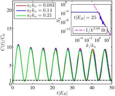
Figure 3: Rescaled Tan’s contact $C(t)/C_{0}$ ($C_{0}=16\pi^{2}a_{f}^{2}n^{2}$) for instantaneous quenches from a non-interacting gas $a_{i}=0$ to different values of the final scattering length $a_{f}$. Inset: momentum distribution $N_{k}(t)$ at a fixed time $t$ and scattering length $a_{f}k_{n}=0.14$.

By increasing the value of the final scattering length $a_{f}$, the time-dependent Bogoliubov approximation eventually loses its validity, primarily because it does not include self-consistently the depletion of the condensate. In Fig. 1(b) we plot the density of particles in the excited states $n_{ex}(t)$ by rescaling the time by the molecular binding energy. In contrast to the case of shallow quenches, we can see that our numerical results, at long enough times, start deviating from the ones obtained within the time-dependent Bogoliubov approximation. This deviation occurs on longer time scales (absolute units) for larger values of $a_{f}$ — in Fig. 1(b) the deviation occurs on shorter time scales for larger values of $a_{f}$ because time is measured in units of $|E_{\text{B}}|^{-1}$. In addition, we find that the amplitude of the coherent atom-molecule oscillations increases as $a_{f}^{3}$ (see Fig. 2) and it reaches $\Delta n_{ex}/n\sim 0.12$ for $a_{f}k_{n}=0.52$. Thus we expect the oscillations to become relevant by increasing the value of $a_{f}$.

We extract the amplitude of the oscillations by averaging over several oscillations after the initial transitory behaviour, and using the standard deviation as the uncertainty — the error bar is too small to be observed in Fig. 2. In addition, we find that the oscillation period is universal $T\simeq 2\pi/|E_{\text{B}}|$ up to $a_{f}k_{n}\lesssim 0.21$, while the medium starts to influence the dynamics by decreasing the period value only for larger interaction strengths (top panel of Fig. 4). Note that, for $a_{f}k_{n}\lesssim 0.21$, $|E_{\text{B}}|^{-1}\lesssim 2~{}\mu$s (see Tab. 1). As commented at the end of Sec. II.2, recent experiments Fletcher et al. (2017); Eigen et al. (2018) have shown that three-body processes and losses are negligible for $t\lesssim\epsilon_{n}^{-1}\sim 80~{}\mu$s and thus there is an interval in the early-time dynamics when we expect that it should be possible to measure coherent atom-molecule oscillations before three-body processes and losses start to affect the dynamics.

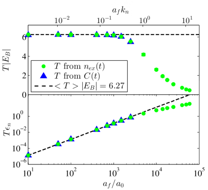
Figure 4: Period $T$ of coherent oscillations extracted from the excited particle density $n_{ex}(t)$ ([green] dots) and from the Tan’s contact $C(t)$ ([blue] triangles) as a function of $a_{f}k_{n}$ ($a_{f}$ in units of the Bohr radius $a_{0}$ is given for a density $n=10^{12}$ cm^-3). Top panel: the period $T$ is plotted in units of the molecular binding energy $|E_{B}|$. Bottom panel: $T$ is plotted in units of the energy scale associated with the gas density $\epsilon_{n}$.

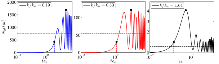
Figure 5: Normalized momentum distribution $\tilde{N}_{{\mathbf{k}}}(t)$ as a function of time $t$ after a diabatic quench to $a_{f}k_{n}=4.1$ (corresponding to $a_{f}=20000a_{0}$ when $n=10^{12}$ cm^-3) for different value of the momentum $k$. The dashed horizontal line represents the value of the mean steady-state $\tilde{N}_{ss}(k)$ reached after an initial quench transient. The dashed vertical line marks the value of the growth time $\tau_{gr}(k)$, defined as the time at which $\tilde{N}_{{\mathbf{k}}}(t)$ reaches $1/4$ of its maximum value ([black] dots) at a given value of $k$.

Finally, we plot in Fig. 1(c) the excited state density for the largest values of $a_{f}$ we can simulate. As explained in App. B, where we discuss the convergence of our results with respect to the number of points $M$ on the Gauss-Legendre momentum grid and the momentum cutoff $\Lambda$, our numerics suffers a critical slowing down of the convergence with respect to both parameters. For this reason, $a_{f}k_{n}=12.4$ ($a_{f}=6\times 10^{4}a_{0}$ and $n=10^{12}$ cm^-3) is the largest value we can simulate to extract converged information in a reasonable running time. In this regime, we find that the excitation density very quickly converges into a steady-state regime with a large average condensate depletion of $\sim 96\%$. In addition, we find that the increase of the period of oscillations $T$ with $a_{f}$ slows down for $a_{f}k_{n}\gtrsim 0.21$. In particular, in Fig. 4 we plot the period of the coherent oscillations, either in units of $|E_{\text{B}}|$ (top panel) or $\epsilon_{n}$ (bottom panel). While the slope of $T\epsilon_{n}$ reduces sensibly, indicating the approach to a universal regime, we cannot enter a universal regime for the period where $T\epsilon_{n}\simeq\text{const}$. At the same time, the period in this regime is $T>\epsilon_{n}^{-1}$ and on this time scale three-body events, heating and losses have been shown to start playing a relevant role in the experiments Fletcher et al. (2017); Eigen et al. (2018), making it difficult to measure the oscillations in $n_{ex}(t)$. However, even though in the unitary regime we neither can disclose a universal behaviour of the oscillation period nor expect this to be accessible experimentally, as we will see later in Sec. III.3, in the unitary regime we find a universal scaling behaviour of the typical growth time $\tau_{gr}$ of the momentum distribution which is a typical time of the very-early gas dynamics ($\tau_{gr}\epsilon_{n}\lesssim 1$).

III.2 Tan’s contact

The momentum distribution of a quantum gas governed by an $s$-wave contact interaction $a$ always decays for large momenta as $k^{-4}$ Tan (2008). The Tan’s contact is thus defined as

$$C=\lim_{k\to\infty}k^{4}N_{\mathbf{k}}\;.$$ (21)

$C$ measures the strength of two-body short-range correlations. For a weakly interacting Bose gas, the Tan’s contact can be easily derived employing the Bogoliubov approximation and is given by $C_{0}=16\pi^{2}a^{2}n^{2}$ Pitaevskii and Stringari (2003). It is possible to show that the momentum distribution retains a $k^{-4}$ large momentum tail also for quantum quenches, and thus one can define an instantaneous Tan’s contact $C(t)$ Corson and Bohn (2015); Yin and Radzihovsky (2016).

As shown in Fig. 3, we extract the time dependence of the Tan’s contact $C(t)$ after instantaneous quenches by fitting the tail of the momentum distribution $N_{{\mathbf{k}}}(t)$ at fixed $t$ (see inset) and plot it for several values of the scattering length $a_{f}$. As for $n_{ex}(t)$, the Tan’s contact also shows coherent oscillations. The oscillation period coincides with that of $n_{ex}(t)$ — see Fig. 4. In addition, we show that there is a a large interval of values of $a_{f}k_{n}\lesssim 0.21$ for which the oscillations are universal both in amplitude (in units of $C_{0}=16\pi^{2}a_{f}^{2}n^{2}$) as well as for the period (in units of $|E_{\text{B}}|^{-1}$) and represent coherent atom-molecule oscillations. As commented in the case of $n_{ex}(t)$, because in this regime $T\simeq 2\pi/|E_{\text{B}}|<\epsilon_{n}^{-1}$, we expect that the coherent atom-molecule oscillations should be measurable by considering the time dependence of the Tan’s contact. However, for larger values of $a_{f}$, eventually the period increases, reaching $T>\epsilon_{n}^{-1}$, and it is thus on time-scales for which the system is affected by three-body effects and losses.

Nevertheless, as discussed in the next section, our Ansatz (8) is still able to describe the very early-time dynamics, and it exposes a universal scaling behaviour of the typical growth time of the momentum distribution, in agreement with recent experiments Eigen et al. (2018).

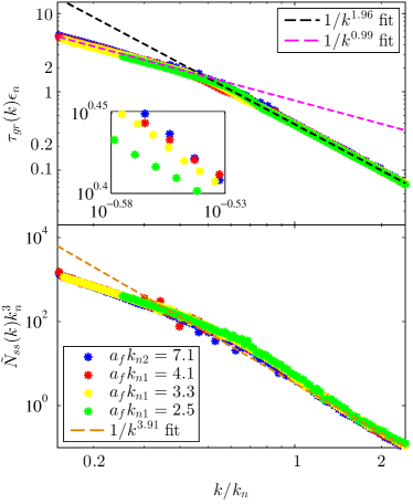
Figure 6: Top panel: Growth time $\tau_{gr}(k)$ of the normalized momentum distribution $\tilde{N}_{{\mathbf{k}}}(t)$ (see Fig. 5) as a function of momentum for different values of $a_{f}$ in the unitary regime and for two densities, $n_{1}=10^{12}$ cm^-3 and $n_{2}=5\times 10^{12}$ cm^-3 (see legend in the bottom panel). Bottom panel: Mean steady-state value $\tilde{N}_{ss}(k)$ reached by the momentum distribution after an initial transient of the quench (see Fig. 5) as a function of momentum for the same values of $a_{f}$ and densities as the top panel.

III.3 Universal prethermal dynamics in the unitary regime

Let us consider the time dependence of the momentum distribution $N_{{\mathbf{k}}}(t)$ after a diabatic quench to $a_{f}$ in the unitary regime. Similarly to Ref. Eigen et al. (2018), we define the normalized momentum distribution, as

$$\tilde{N}_{{\mathbf{k}}}(t) =\displaystyle\frac{N_{{\mathbf{k}}}(t)}{n_{ex}(t)} \displaystyle\frac{1}{V}\displaystyle\operatorname*{\bar{\sum}}_{\mathbf{k}}\tilde{N}_{{\mathbf{k}}}(t) =1\;.$$ (22)

In Fig. 5 we plot $\tilde{N}_{{\mathbf{k}}}(t)$ as a function of time for different values of the momentum $k$. Immediately after the quench, the momentum distribution grows rapidly as $\propto t^{3/2}$. We want to determine the typical growth time $\tau_{gr}(k)$ of the momentum distribution at a fixed momentum. To this end, we identify, at each fixed momentum $k$, the maximum value of $\tilde{N}_{{\mathbf{k}}}(t)$ and define $\tau_{gr}(k)$ ([black] dashed vertical line) as the time at which $\tilde{N}_{{\mathbf{k}}}(\tau_{gr})$ reaches a fixed percentage of the maximum value. We choose this to be $1/4$, but our results are independent of this value, as long as $\tau_{gr}$ lies in the tail of the growing region of $\tilde{N}_{{\mathbf{k}}}(t)$ that is not affected by the oscillatory behaviour yet. In fact, after the transient, the momentum distribution enters a steady-state regime dominated by large coherent oscillations around a steady state value $\tilde{N}_{ss}(k)$ ([black] dashed horizontal line). Note that these are not atom-molecule oscillations only because now they involve the entire medium, as suggested by the fact that their period $T$ moves away from $2\pi/|E_{\text{B}}|$ and starts to saturate towards $\propto\epsilon_{n}^{-1}$.

The presence of large oscillations represents a substantial difference from the experimental results of Ref. Eigen et al. (2018) where highly damped oscillations are barely visible in the prethermal dynamics and where the normalized momentum distribution quickly approaches a steady state value after an almost monotonic initial growth. For this reason, the authors of Ref. Eigen et al. (2018) can apply a sigmoid fit to extract the growth time $\tau_{gr}(k)$ there defined as the time at which the momentum distribution reaches $1/2$ of the steady-state value $\tilde{N}_{ss}(k)$. Even by averaging out the coherent oscillations in our results for $\tilde{N}_{{\mathbf{k}}}(t)$, we cannot apply a sigmoid fit to our data because, at large momenta, the growth towards the steady-state prethermal regime is not monotonic (see the last panel of Fig. 5). For this reason we have applied the criterion previously described to extract the growth time $\tau_{gr}(k)$.

Nevertheless, by plotting in the top panel of Fig. 6 the rescaled growth time $\tau_{gr}(k)\epsilon_{n}$ as a function of the rescaled momentum $k/k_{n}$ we disclose, in agreement with the experiments Eigen et al. (2018), a universal scaling behaviour which is independent of both the final scattering length $a_{f}$ and the gas density $n$. In particular, the value extracted for $\tau_{gr}(k)$ at different values of $a_{f}k_{n}>2.5$ and at two different gas densities, fall onto the same universal curve. As in Eigen et al. (2018), the fitting of our data reveals the following universal scaling laws for small and large momenta:

$$\begin{split}\tau_{gr}(k)\epsilon_{n}&\operatorname*{\simeq}_{k<k_{n}}\displaystyle\frac{k_{n}}{k}\\ \tau_{gr}(k)\epsilon_{n}&\operatorname*{\simeq}_{k>k_{n}}\left(\displaystyle\frac{k_{n}}{k}\right)^{2}\;.\end{split}$$ (23)

We have checked that this result is independent of the specific percentage of the maximum value of $\tilde{N}_{{\mathbf{k}}}(t)$ chosen to define $\tau_{gr}(k)$ — a different percentage just scales rigidly all those curves up or down, leaving unchanged the universal scaling behaviour.

Note that for shallow quenches one can also define a typical growth time $\tau_{gr}^{Bog}(k)$ of the momentum distribution and a steady state value $\tilde{N}_{ss}^{Bog}(k)$ that characterizes the long-time dynamics of the momentum distribution. Starting from the analytic expression (29) for $g_{{\mathbf{k}}}(t)$ obtained within the time-dependent Bogoliubov approximation, one can deduce the following expressions:

$$\displaystyle\frac{\tau^{Bog}_{gr}(k)}{\tau} =\frac{\pi}{6E_{k}\tau} \displaystyle\frac{\tilde{N}_{ss}^{Bog}(k)}{\xi^{3}} =\frac{\sqrt{2^{5}}\pi}{(E_{k}\tau)^{2}}\;.$$ (24)

The dependence on the momentum $k$ of both quantities reveals information about the Bogoliubov spectrum of quasi-particle excitations of a weakly interacting Bose gas, $E_{k}\tau=\sqrt{(k\xi)^{2}[(k\xi)^{2}+2]}$. As in Eq. (23), the result for the growing time $\tau^{Bog}_{gr}(k)$ give the same rescaling with momentum, i.e., at low momenta $k\xi\ll 1$, $\tau^{Bog}_{gr}(k)/\tau\simeq(k\xi)^{-1}$, while in the opposite regime $k\xi\gg 1$, $\tau^{Bog}_{gr}(k)/\tau\simeq(k\xi)^{-2}$. This corresponds to the phonon and free particle regimes of the Bogoliubov spectrum, respectively. In the strongly interacting regime, we thus find the very same universal regime but with the mean-field energy $\tau^{-1}$ replaced by “Fermi” energy $\epsilon_{n}$ and the healing length $\xi$ by $k_{n}^{-1}$. This thus indicates that the excitations spectrum is still phonon-like for small momenta and free-like at higher momenta, but with energy and momentum scales only determined by the gas density. The agreement with the experiments on the universal scaling law of the growth time $\tau_{gr}^{Bog}(k)$ indicates that the very-early-time quench dynamics into the unitary regime, when a stationary prethermal regime has not been reached yet, is dominated by excitations of atoms out of the condensate in pairs only.

We plot in the bottom panel of Fig. 6 the mean steady-state value $\tilde{N}_{ss}(k)$ reached by the momentum distribution after the initial transient after the initial growth as a function of momentum. Like in the experiments, we also find a universal behaviour of this quantity in units of $k_{n}$. However, in contrast with experiments for which this quantity follows a single exponential law, our calculations reveal a crossover to a power-law $k^{-4}$ decay for large values of momenta. This is expected for a dissipationless quantum gas governed by an $s$-wave contact interaction, and leads to the extraction of the Tan’s contact. This indicates that, for quenches into the unitary regime, once the very early-time growth and transient dynamics of the momentum distribution has passed and the system enters the prethermal region, our dissipationless description which leads to strong coherent oscillations around a steady-state value is incomplete.

IV Conclusions

We have analyzed the crossover from shallow to deep instantaneous interaction quenches in the early-time dynamics of a degenerate Bose gas at zero temperature. We have employed a time-dependent Nozières-Saint James variational formalism, which self-consistently describes the excitation of particles out of the condensate in pairs only. We have modelled short-range atom interactions close to a Feshbach resonance using a single-channel model, which admits a molecular bound state on the repulsive side of the resonance. The coupled dynamics between the condensate and the excited states includes the condensate depletion and correlations between non-condensed atoms.

In agreement with previous studies Sykes et al. (2014); Corson and Bohn (2015), we have found coherent atom-molecule oscillations in both the density of excited particles and the Tan’s contact, and we have characterized them as a function of the final scattering length $a_{f}$. For shallow quenches, the oscillations have a negligible amplitude and the dynamics is well captured by a time-dependent Bogoliubov theory Natu and Mueller (2013); Hung et al. (2013), involving the mean-field time and the healing length. However, at intermediate values of the final scattering length $a_{f}k_{n}\lesssim 0.21$, we find a universal regime for atom-molecule oscillations, where the period is only determined by the molecular binding energy, $T\simeq 2\pi/|E_{\text{B}}|$, and the amplitude of oscillations is not negligible. We expect such oscillations to be visible in experiments, since recent experiments on ³⁹K have shown that three-body processes and losses are negligible for $t\lesssim\epsilon_{n}^{-1}\sim 80~{}\mu$s Eigen et al. (2018), while $|E_{\text{B}}|^{-1}\lesssim 2~{}\mu$s.

We have pushed our analysis into the unitary regime and we can simulate the dynamics up to $a_{f}k_{n}=12.4$. Here we find that the growth time of the momentum distribution $\tau_{gr}(k)$, which characterizes the very-early-time quench dynamics, depends on the momentum $k$ with a universal scaling law that is governed by density only. In particular, we can deduce that, at very short times after the quench, the excitations are Bogoliubov modes with the mean-field energy $\tau^{-1}$ replaced by $\epsilon_{n}$ and the healing length $\xi$ by $k_{n}^{-1}$. During these very-early times after the quench, where the momentum distribution has not yet entered a prethermal regime, the agreement between our results and the experiments indicates that higher-order incoherent processes do not affect the postquench behaviour at short times and thus, the employment of a time-dependent Nozières-Saint James variational formalism is adequate in this case. However, the very strong damping of the coherent oscillations observed in experiments when the quench dynamics enters the prethermal regime, indicates that damping and dissipation mechanisms should eventually be taken into account. This is further confirmed by the observation of an exponential behaviour of the mean steady-state value $\tilde{N}_{ss}(k)$ reached by the momentum distribution in the prethermal regime Eigen et al. (2018), while instead our model predicts a typical power-law $k^{-4}$ decay for large values of momenta.

One way to include damping and dissipation would be to consider a phenomenological model, as in Ref. Rançon and Levin (2014), where the system is coupled to an external bath, thus allowing energy to dissipate. Alternatively, one could consider the next order term in the time-dependent variational Ansatz (8) which allows the excitations of particles out of the condensate in triplets. The inclusion of this term would allow one to incorporate the effects of Beliaev decay, Landau scattering Van Regemortel et al. (2018) and potentially even Efimov physics. This will be the subject of future studies.

Appendix A Shallow quenches

For shallow interaction quenches, $na_{i,f}^{3}\ll 1$, the dynamics is integrable and one can solve exactly (13) and (14), recovering the results of Refs. Natu and Mueller (2013); Hung et al. (2013). In this limit, the contribution from $\langle\hat{H}_{4}\rangle$ (12) can be neglected and one can replace the bare interactions with inverse zero-energy T matrix, giving the interaction strength $U_{i,f}=4\pi a_{i,f}/m$. Moreover one can assume the condensate depletion is negligible, $|c_{0}(t)|^{2}\simeq n$, and thus the equation of motions can be simplified to:

$$i\dot{c}_{0} \simeq U_{f}c_{0}n$$ (25)

$$i\dot{g}_{\mathbf{k}} =2\left[\epsilon_{\mathbf{k}}+2U_{f}n\right]g_{\mathbf{k}}+U_{f}\left(g_{\mathbf{k}}^{2}c^{*2}_{0}+c^{2}_{0}\right)\;.$$ (26)

It is easy to show that these equations are solved exactly by

$$c_{0}(t) =\sqrt{n}e^{-iU_{f}nt}$$ (27)

$$g_{\mathbf{k}}(t) =\bar{g}_{\mathbf{k}}(t)e^{-2iU_{f}nt}$$ (28)

$$\bar{g}_{\mathbf{k}}(t) =\frac{E_{\mathbf{k}f}g_{\mathbf{k}}(0)-i\tan(E_{\mathbf{k}f}t)[U_{f}n+\xi_{\mathbf{k}f}g_{\mathbf{k}}(0)]}{E_{\mathbf{k}f}+i\tan(E_{\mathbf{k}f}t)[\xi_{\mathbf{k}f}+U_{f}ng_{\mathbf{k}}(0)]}\;,$$ (29)

where $E_{\mathbf{k}f}=\sqrt{\epsilon_{{\mathbf{k}}}(\epsilon_{{\mathbf{k}}}+2U_{f}n)}$ is the quasi-particle excitation spectrum and $\xi_{\mathbf{k}f}=\epsilon_{{\mathbf{k}}}+U_{f}n$.

This coincides with the result obtained in Refs. Natu and Mueller (2013); Hung et al. (2013) by using a time-dependent Bogoliubov approximation, where one considers the Heisenberg equations of motion for the particle operator $\hat{a}_{{\mathbf{k}}}(t)$,

$$i\displaystyle\frac{d\hat{a}_{{\mathbf{k}}}}{dt}=[\hat{a}_{{\mathbf{k}}},\sum_{\mathbf{k}}\epsilon_{\mathbf{k}}\hat{a}_{{\mathbf{k}}}^{\dagger}\hat{a}_{{\mathbf{k}}}+\hat{H}_{2}]\;.$$

This equation is solved in terms of the Bogoliubov parameters, $\hat{a}_{{\mathbf{k}}}=u_{{\mathbf{k}}}(t)\hat{b}_{{\mathbf{k}}}+v_{{\mathbf{k}}}^{*}(t)\hat{b}_{-{\mathbf{k}}}^{{\dagger}}$, where $|u_{{\mathbf{k}}}(t)|^{2}-|v_{{\mathbf{k}}}(t)|^{2}=1$, giving:

$$i\displaystyle\frac{d}{dt}\begin{pmatrix}u_{{\mathbf{k}}}(t)\\ v_{{\mathbf{k}}}(t)\end{pmatrix}=\begin{pmatrix}\xi_{{\mathbf{k}}f}&U_{f}n\\ -U_{f}n&-\xi_{{\mathbf{k}}f}\end{pmatrix}\begin{pmatrix}u_{{\mathbf{k}}}(t)\\ v_{{\mathbf{k}}}(t)\end{pmatrix}\;.$$

It is easy to show that these coupled equations are solved by

$$\bar{g}_{{\mathbf{k}}}(t) =\displaystyle\frac{v_{{\mathbf{k}}}^{*}(t)}{u_{{\mathbf{k}}}^{*}(t)} |u_{{\mathbf{k}}}(t)| =\displaystyle\frac{1}{\sqrt{1-|\bar{g}_{{\mathbf{k}}}(t)|^{2}}}\;,$$ (30)

and one recovers, e.g. for the fraction of particles in the excited states, the result of Natu and Mueller (2013):

$$n_{ex}^{Bog}(t)\xi^{3}=\frac{1}{2\pi^{2}}\int_{0}^{\tilde{\Lambda}}\tilde{k}^{2}d\tilde{k}\Biggl{[}\frac{|g_{k}(0)|^{2}}{1-|g_{k}(0)|^{2}}\\ -\left(\frac{a_{i}}{a}-1\right)\frac{\sin^{2}\left(\sqrt{\tilde{k}^{2}(\tilde{k}^{2}+2)}\tau\right)}{(\tilde{k}^{2}+2)\sqrt{\tilde{k}^{2}(\tilde{k}^{2}+2a_{i}/a)}}\Biggr{]}\;.$$ (31)

Figure 7: Two-step extrapolation process of the period of oscillations $T$ of the non-condensed density $n_{ex}(t)$ (Fig. 1) with respect to the two system regularisation parameters, $M$ and $\Lambda$. The period $T$ ([blue] dots) is evaluated, at fixed values of $M$ and $\Lambda$, by averaging over several oscillations of $n_{ex}(t)$, with an error given by the standard deviation (not observed in these plots). Top panel: $T$ is plotted as a function of $M^{-1}$ for a fixed value of $\Lambda/k_{n}=513$. The $M\to\infty$ value $T_{M\to\infty}$ is extracted via an exponential fit ([red] solid line). Bottom panel: Plot of the extracted period $T_{M\to\infty}$ with respect to $\Lambda^{-1}$ ([blue] dots). The extrapolated value $T_{M\to\infty,\Lambda\to\infty}$ is obtained via a linear fit ([red] solid line). We have fixed $n=10^{12}$ cm^-3 and $a_{f}=1000a_{0}$ ($a_{f}k_{n}=0.21$).

Appendix B Convergence of the dynamics

We show here the convergence of our results with respect to the number of points $M$ on the Gauss-Legendre momentum grid and the momentum cutoff $\Lambda$. Note that, as the dynamics requires in principle one regularization parameter only, we could send $\Lambda\to\infty$ and use only the number of points $M$ to regularize Eq. (2). However, we could not obtain results converged in time applying this procedure. For this reason, we have fixed both $M$ and $\Lambda$ in our numerics and checked the convergence with respect to both parameters.

We show here the extrapolation procedure followed to extract the $M\to\infty$ and $\Lambda\to\infty$ results for the oscillation period $T$ of the non-condensed density $n_{ex}(t)$. Convergence with respect to both parameters has been checked for all data reported in the main text. We have found that the dynamics converges exponentially fast with respect to the number of Gauss-Legendre points $M$ used for the quadrature, while it only has a linear dependence on the cutoff $\Lambda$ (for the range of $\Lambda$ values computationally accessible). Fig. 7 shows the dependence of the period of oscillations with respect to both $M$ (top panel) and $\Lambda$ (bottom panel). Once we have extracted $T_{M\to\infty}$ for different values of $\Lambda$, we can extract the final value $T_{M\to\infty,\Lambda\to\infty}$ reported in Fig. 4. The numerical calculations are limited by a critical slowing down of the convergence with respect to the regularization parameters for both very small and very large values of $a_{f}$.

References

- Chin et al. (2010) C. Chin, R. Grimm, P. Julienne, and E. Tiesinga, Rev. Mod. Phys. 82, 1225 (2010).
- Fletcher et al. (2013) R. J. Fletcher, A. L. Gaunt, N. Navon, R. P. Smith, and Z. Hadzibabic, Phys. Rev. Lett. 111, 125303 (2013).
- Rem et al. (2013) B. S. Rem, A. T. Grier, I. Ferrier-Barbut, U. Eismann, T. Langen, N. Navon, L. Khaykovich, F. Werner, D. S. Petrov, F. Chevy, and C. Salomon, Phys. Rev. Lett. 110, 163202 (2013).
- Makotyn et al. (2014) P. Makotyn, C. E. Klauss, D. L. Goldberger, E. A. Cornell, and D. S. Jin, Nature Physics 10, 116 (2014).
- Eismann et al. (2016) U. Eismann, L. Khaykovich, S. Laurent, I. Ferrier-Barbut, B. S. Rem, A. T. Grier, M. Delehaye, F. Chevy, C. Salomon, L.-C. Ha, and C. Chin, Phys. Rev. X 6, 021025 (2016).
- Klauss et al. (2017) C. E. Klauss, X. Xie, C. Lopez-Abadia, J. P. D’Incao, Z. Hadzibabic, D. S. Jin, and E. A. Cornell, Phys. Rev. Lett. 119, 143401 (2017).
- Lopes et al. (2017) R. Lopes, C. Eigen, A. Barker, K. G. H. Viebahn, M. Robert-de Saint-Vincent, N. Navon, Z. Hadzibabic, and R. P. Smith, Phys. Rev. Lett. 118, 210401 (2017).
- Fletcher et al. (2017) R. J. Fletcher, R. Lopes, J. Man, N. Navon, R. P. Smith, M. W. Zwierlein, and Z. Hadzibabic, Science 355, 377 (2017).
- Eigen et al. (2017) C. Eigen, J. A. P. Glidden, R. Lopes, N. Navon, Z. Hadzibabic, and R. P. Smith, Phys. Rev. Lett. 119, 250404 (2017).
- Eigen et al. (2018) C. Eigen, J. A. P. Glidden, R. Lopes, E. A. Cornell, R. P. Smith, and Z. Hadzibabic, Nature 563, 221 (2018).
- Hung et al. (2013) C.-L. Hung, V. Gurarie, and C. Chin, Science 341, 1213 (2013).
- Efimov (1970) V. Efimov, Physics Letters B 33, 563 (1970).
- Braaten and Hammer (2006) E. Braaten and H.-W. Hammer, Physics Reports 428, 259 (2006).
- Smith et al. (2014) D. H. Smith, E. Braaten, D. Kang, and L. Platter, Phys. Rev. Lett. 112, 110402 (2014).
- Yin and Radzihovsky (2013) X. Yin and L. Radzihovsky, Phys. Rev. A 88, 063611 (2013).
- Sykes et al. (2014) A. G. Sykes, J. P. Corson, J. P. D’Incao, A. P. Koller, C. H. Greene, A. M. Rey, K. R. A. Hazzard, and J. L. Bohn, Phys. Rev. A 89, 021601 (2014).
- Rançon and Levin (2014) A. Rançon and K. Levin, Phys. Rev. A 90, 021602 (2014).
- Kain and Ling (2014) B. Kain and H. Y. Ling, Phys. Rev. A 90, 063626 (2014).
- Corson and Bohn (2015) J. P. Corson and J. L. Bohn, Phys. Rev. A 91, 013616 (2015).
- Kira (2015) M. Kira, Nature Communications 6 (2015).
- Ancilotto et al. (2015) F. Ancilotto, M. Rossi, L. Salasnich, and F. Toigo, Few-Body Systems 56, 801 (2015).
- Yin and Radzihovsky (2016) X. Yin and L. Radzihovsky, Phys. Rev. A 93, 033653 (2016).
- Nozières, P. and Saint James, D. (1982) Nozières, P. and Saint James, D., J. Phys. France 43, 1133 (1982).
- Natu and Mueller (2013) S. S. Natu and E. J. Mueller, Phys. Rev. A 87, 053607 (2013).
- Van Regemortel et al. (2018) M. Van Regemortel, H. Kurkjian, M. Wouters, and I. Carusotto, Phys. Rev. A 98, 053612 (2018).
- Gurarie and Radzihovsky (2007) V. Gurarie and L. Radzihovsky, Annals of Physics 322, 2 (2007).
- Song and Zhou (2009) J. L. Song and F. Zhou, Phys. Rev. Lett. 103, 025302 (2009).
- Parish and Levinsen (2016) M. M. Parish and J. Levinsen, Phys. Rev. B 94, 184303 (2016).
- Kramer (2008) P. Kramer, Journal of Physics: Conference Series 99, 012009 (2008).
- Pitaevskii and Stringari (2003) L. Pitaevskii and S. Stringari, Bose-Einstein Condensation, International Series of Monographs on Physics (Clarendon Press, 2003).
- Donley et al. (2002) E. A. Donley, N. R. Claussen, S. T. Thompson, and C. E. Wieman, Nature 417, 529 (2002).
- Claussen et al. (2003) N. R. Claussen, S. J. J. M. F. Kokkelmans, S. T. Thompson, E. A. Donley, E. Hodby, and C. E. Wieman, Phys. Rev. A 67, 060701 (2003).
- Tan (2008) S. Tan, Annals of Physics 323, 2952 (2008).