Theoretical foundation of detrending methods for fluctuation analysis such as detrended fluctuation analysis and detrending moving average

Abstract

We present a general framework of detrending methods of fluctuation analysis of which detrended fluctuation analysis (DFA) is one prominent example. Another more recently introduced method is detrending moving average (DMA). Both methods are constructed differently but are similarly able to detect long-range correlations as well as anomalous diffusion even in the presence of nonstationarities. In this article we describe their similarities in a general framework of detrending methods. We establish this framework independently of the definition of DFA or DMA but by investigating the failure of standard statistical tools applied on nonstationary time series, let these be intrinsic nonstationarities such as for Brownian pathes, or external ones due to additive trends. In particular, we investigate the sample averaged mean squared displacement of the summed time series. By modifying this estimator we introduce a general form of the so-called fluctuation function and can formulate the framework of detrending methods. A detrending method provides an estimator of the fluctuation function which obeys the following principles: The first relates the scaling behaviour of the fluctuation function to the stochastic properties of the time series. The second principles claims unbiasedness of the estimatior. This is the centerpiece of the detrending procedure and ensures that the detrending method can be applied to nonstationary time series, e.g. FBM or additive trends. Both principles are formulated and investigated in detail for DFA and DMA by using the relationship between the fluctuation function and the autocovariance function of the underlying stochastic process of the time series.

I Introduction

Long-range temporal correlations are omnipresent in a tremendous amount of data sets and pose an ongoing challenge in time series analysis since its first empirical detection by H. E. Hurst analyzing river flows hurst . For an excellent overview about the research history see graves . Long-range correlations reflect some memory in a time series recorded from a complex system and express themselves usually by a power-law decay of the autocorrelation function. Especially in nonstationary time series the existence of long-range correlations have a non-negligible impact on the analysis, modelling and prediction of these series, see palma ; beran ; pipiras . Several traditional methods for the detection of the correlation structure fail in the presence of nonstationarities such as additive polynomial trends. These methods include the sample estimation of the autocorrelation function, the R/S analysis hurst and the fluctuation analysis kantelhardt2 . Hence advanced methods are required in order to detect reliably long-range correlations in nonstationary time series.

A very popular and frequently used method for the quantitative characterizaton of long range correlations is detrended fluctuation analysis (DFA) introduced by Peng et al. analysing DNA sequences peng . For a good introduction see kantelhardt2 . DFA has been applied to many diverse fields such as heart rate variability penzel ; echeverria ; castiglioni ; baumert , air temperature talkner ; kiraly ; kurnaz ; bunde ; meyer ; massah , hydrology hurst ; zhang ; zhang3 , cloud breaking ivanova , sea surface temperature luo , stock prices cao ; reboredo ; serletis and oil markets ramirez ; wang . The continuing success of DFA can be explained by its easy construction as well as its well-perfoming results taqqu2 ; hu ; chen ; chen2 ; xu ; bashan ; ma ; weron . In addition, DFA has been developed further to also analyse multifractality kantelhardt ; movahed ; movahed2 ; zhang2 ; zhou ; zhou2 and cross-correlations podobnik ; zhou3 ; horvatic . Another more recently developed method is called detrending moving average (DMA), see alessio ; arianos2 and for a good overview see carbone4 . This method is also well-performing xu ; bashan ; carbone2 ; carbone3 ; carbone5 ; shao with strong applications in analyzing financial data carbone6 ; dimatteo ; serletis2 ; matsuhita ; serletis3 and fractal structures carbone7 ; carbone8 ; turk . In kiyono4 a fast algorithm has been proposed which drastically decreases the computation time of DMA. Although DFA and DMA are constructed differently their basic principles are working similarly in the time domain. We refer to these two methods as detrending methods for fluctuation analysis in this article. Yet another powerful method is based on a wavelet-transform of a given time series and was introduced by abry ; veitch , and we will later also discuss its relationship to DFA and DMA. This relationship has already been investigated by kiyono5 for stationary processes.

We focus here on detrending methods for fluctuation analysis which are modified random walk analysis where the time series is interpreted as increment process of a random walk like path. These methods provide an estimator of the so-called fluctuation function whose scaling behaviour is directly related to the correlation type of the time series. The implementation of detrending methods consists of several straightforward steps transforming resulting in an estimator of the fluctuation function. Hereby one crucial part of the procedure is the trend elimination of the path in segments of the time axis, called “detrending”. Since the detrending in DFA and DMA is ad hoc, it is by far not obvious how the fluctuation function is connected to the correlation structure.

The current analytical understanding of DFA and DMA is at a different states. To our best knowledge analytical studies of DMA exist for the derivation of the scaling behaviour for fractional Gaussian noise arianos2 ; arianos ; carbone and on the ability of removing additive trends carbone . In contrast there exist relatively more analytical studies of DFA which can be classified into four categories: 1) Calculation of the scaling behaviour of the fluctuation function for specific process, namely autoregressive model of first order hoell , fractional Gaussian noise hoell2 ; taqqu2 ; bardet ; movahed2 ; crato and FBM movahed ; heneghan ; kiyono ; 2) Derivation of the relationship between the fluctuation function and known statistical quantities, namely the autocorrelation function hoell2 , power spectrum heneghan ; kiyono ; kiyono2 ; kiyono3 ; talkner ; willson ; willson2 and variogram lovstetten ; 3) Describing statistical properties of the fluctuation function bardet ; crato ; 4) Illuminating the functionality of detrending hoell3 . Nevertheless there are still many open questions about these methods, see for example kiyono3 ; bryce , not just about minor technical details but questions about fundamental principles and properties of detrending methods. We know that detrending methods work for a large class of nonstationary processes but we are ignorant of why they work. This is actually rather suprising since the operation of detrending is the centrepiece of detrending methods. Since detrending is usually done on segments of the time series, it leads to mutually inconsistent local trends, and never reproduces a given global, e.g., linear trend on data.

In this article, we present an intuitive and natural motivation of detrending methods and also demonstrate in detail how they work for different types of nonstationarities. In order to accomplish this goal it is essential to derive the general relationship between the fluctuation function and the autocovariance function. Hence this article is constructed as follows. In Sec. 2 we recapitulate problems of the sample autocovariance function in the presence of long-range correlations and nonstationarities. We argue that the mean squared displacement of the random walk path provides a better tool to analyze the correlation structure of a time series. In Sec. 3 we show that the estimator of this mean squared displacement requires stationary increments which is only fulfilled for stationary time series. We demonstrate the failure of the estimator in analyzing the scaling behaviour for two different types of nonstationarity, namely intrinsic and external nonstationarity. In Sec. 4 we introduce the general framework of detrending methods and formulate two basic principles which must be fulfilled in order to estimate reliably the correlation structure. In Sec. 5 we discuss that DFA and DMA are indeed specific realizations of the general framework of detrending methods. Here we only focus on centered DMA and not backward and forward DMA. In Sec. 6 we explicitely show that DFA and DMA fulfill the two principles of detrending methods.

II Basics and motivation

II.1 Autocorrelation function

Given is a time series $\{x(t)\}_{t=1}^{N}$. We understand this time series as a superposition of a single realisation of a stochastic process $\{\epsilon(t)\}_{t=1}^{N}$ and a deterministic function $\{m(t)\}_{t=1}^{N}$ given as

$$x(t)=\epsilon(t)+m(t).$$ (1)

We restrict ourselves to Gaussian stochastic processes with time independent zero mean. $\{\epsilon(t)\}_{t=1}^{N}$ is a realisation of an either discrete or a continuous process, where the latter is sampled at discrete times. The stochastic process itself can be stationary or nonstationary. For the sake of simplicity we use in the following the notation $\{\epsilon(t)\}_{t=1}^{N}$ for either a stochastic process or a single realisation and mention accordingly which of them we mean. Therefore we also use $\{x(t)\}_{t=1}^{N}$ for the combination of a deterministic function $m(t)$ and either a stochastic process or a single realisation. Usually, $m(t)$ is a polynomial in $t$ but it can also be any other non-stochastic function such as being periodic.

Let us first assume that the stochastic process is stationary. The autocorrelation function

$$C(\tau)=\frac{\text{Cov}(\tau)}{\text{Cov}(0)}=\frac{\langle\epsilon(t)\epsilon(t+\tau)\rangle}{\langle\epsilon^{2}(t)\rangle}$$ (2)

is a relevant characteristic. If the stochastic process is nonstationary then the autocovariance function depends on both time points $\text{Cov}(i,j)=\langle\epsilon(i)\epsilon(j)\rangle$.

There are two important classes of correlation types depending on the behaviour of the autocorrelation function for large time lags $\tau$: short-range correlations and long-range correlations. A short-range correlated processes has a finite characteristic correlation time $s_{c}=\int_{0}^{\infty}C(\tau)\mathrm{d}\tau<\infty$ which is characterised by the convergence of the sum of the autocorrelation function over all time lags $\sum_{\tau=0}^{\infty}C(\tau)<\infty$. Notably the uncorrelated white noise process with zero mean and unit variance is included in the class of short-range correlated processes. If on the other the sum diverges $\sum_{\tau=0}^{\infty}C(\tau)=\infty$ then the process is long-range correlated. Hence there exists no characteristic correlation time. Such processes forget their initial conditions very slowly which is known as long memory. Long-range correlations are often described by a decreasing power law of the autocorrelation function

$$C(\tau)\sim\tau^{-\gamma}$$ (3)

with correlation parameter $0<\gamma<1$. An important theoretical model is fractional Gaussian Noise (FGN), see mandelbrot . FGN is the stationary increment process of the self-similar fractional Brownian motion (FBM) with self-similarity parameter $H$. This parameter is often called Hurst parameter and can have the values $1/2<H<1$. We exclude here the anticorrelated regime $0<H<1/2$. Note that the self-similarity parameter and the Hurst parameter are actually different chen3 but for the here studied processes with Gaussian and stationary increments both are equivalent. The relationship between $H$ and the correlation parameter of Eq. (3) is $\gamma=2-2H$. In the special case of $H=1/2$ FBM is the standard Brownian motion (BM).

In order to decide weither or not a given time series is long-range correlated the autocorrelation function in Eq.(2) has to be estimated. This can be done straightforwardly with the sample estimator of the autocorrelation function. The numerator and denominator in Eq.(2) is estimated with the sample estimator of the autocovariance function

$$\widehat{\text{Cov}}_{\text{sample}}(\tau)=\frac{1}{N-\tau}\sum_{i=1}^{N-\tau}x(i)x(i+\tau)$$ (4)

where products of the time series $x(i)x(i+\tau)$ are averaged over all possible time points $i$ for a given time lag $\tau$. Usually one replaces $x(t)$ by $x(t)-\bar{x}(t)$ with the sample mean $\bar{x}(t)$. Unfortunately the estimator $\widehat{\text{Cov}}_{\text{sample}}(\tau)$ has at least two important estimation problems:

• The estimator $\widehat{\text{Cov}}_{\text{sample}}(\tau)$ fluctuates strongly around zero for large $\tau$. This is even the case for only positive values of the true autocovariance function. This statistical uncertainty makes it very difficult to observe a power law $\tau^{-\gamma}$ in the log-log plot which is even worse for short time series.

• The estimator $\widehat{\text{Cov}}_{\text{sample}}(\tau)$ is only meaningful for stationary time series. It can be furthermore even misleading in the sense that this estimator applied to the supperposition of a stationary short-range correlated stochastic processes and a linear trend can show a power law behaviour. This will eventually be misinterpreted as a stationary long-range correlated process, see hoell ; maraun .

A direct estimation of the autocorrelation function is often not possible due to the estimation problems (E1) and (E2). Hence it is reasonable to gain indirectly access to the correlation behaviour using different approaches. We introduce in this article our framework of so-called detrending methods as possible solution of the estimation problems (E1) and (E2). DFA and DMA are examples of these detrending methods. Although it is known that these methods can overcome the problems (E1) and (E2) it lacks until today of both an intuitive understanding as well as a rigorous description. We present in the following basic ideas deduced from well-known mathematical functions and hope we can contribute to the fundamental understanding of the nature of detrending methods.

II.2 Mean squared displacement of the path

To tackle the first estimation problem (E1) we consider the mean squared displacement (MSD) of the path of the stochastic process $\{r(t)\}_{t=1}^{N}$. We define this path as the cumulative sum of the stochastic process

$$r(t)=\sum_{i=1}^{t}\epsilon(i)$$ (5)

so that the stochastic process $\{\epsilon(t)\}_{t=1}^{N}$ is the increment process of $\{r(t)\}_{t=1}^{N}$. If the stochastic process is WN then the path is the standard random walk. The correlation type of the stochastic process, assuming a finite second moment $\langle\epsilon^{2}(t)\rangle$ and stationarity, can be directly connected to the scaling behaviour in $s$ of the path MSD

$$R^{2}(s)=\langle(r(s)-r(0))^{2}\rangle=\langle r^{2}(s)\rangle$$ (6)

which is the mean of the squared displacement with $r(0)=0$. We call this equation the path representation of the path MSD because we will later also introduce a second representation with respect to the increments $\{\epsilon(t)\}_{t=1}^{N}$. Here $s$ is the time covered by the path. In numerical estimates, it should be less than the length of the time series $s\leq N$. The path MSD scales increasingly like

$$R^{2}(s)\sim s^{2\alpha}$$ (7)

with the so-called fluctuation parameter $\alpha$ which will be explained as follows. First we consider stationary stochastic processes. If the stochastic processes is white noise (WN) then the path is BM. Hence the path MSD scales linearly, $R^{2}(s)\sim s$. If the time series is FGN with $1/2<H<1$ then the path is FBM. Hence the path MSD scales super-diffusively $R^{2}(s)\sim s^{2H}$. Although we present here only WN and FGN, processes with an autoregressive part have the same asymptotic scaling behaviour. They can be modeled by an AR($1$) process in the case of short-range correlations and an ARFIMA($1$,$d$,$0$) process in the case of long-range correlations. But then only for large enough $s$ the scaling of $\alpha$ is described as above due to the existence of a larger scaling regime for small $s$. This crossover behaviour requires large data sets in order to observe the correct scaling. Summarizing, for stationary stochastic processes the knowledge of $\alpha$ in Eq. (7) allows us to distinguish between short-range and long-range correlations.

Interestingly, the path MSD contains also information when the stochastic process is nonstationary, whereas for the autocorrelation function stationarity has to be assumed. This means that the path MSD can show anomalous diffusive scaling. We depict this with BM and FBM. If the series is BM then the path is summed BM. Hence the path MSD scales cubically $R^{2}(s)\sim s^{3}$, see hoell . If the series is FBM with $1/2<H<1$ then the path is summed FBM. Hence the path MSD scales like $R^{2}(s)\sim s^{2H+2}$, see taqqu2 . We exclude here the anticorrelated case $0<H<1/2$. So the scaling of the path MSD $R^{2}(s)$ allows us to distinguish between a large class of stochastic processes, stationary and nonstationary, by the value of the fluctuation parameter

$$\alpha\in\begin{cases}\{1/2\}&\text{ for WN},\\ (1/2,1)&\text{ for FGN with }\alpha=H,\\ \{3/2\}&\text{ for BM},\\ (3/2,2)&\text{ for FBM with }\alpha=H+1\end{cases}$$ (8)

with $1/2<H<1$, see figure 1. To be precise, the type of nonstationarity which is exhibited by BM and FBM is called intrinsic, see hoell3 . This means that for a pure noise driven time series $x(t)=\epsilon(t)$ the nonstationarity comes from the nonstationary stochastic process $\{\epsilon(t)\}_{t=1}^{N}$. A second type of nonstationarity introduced in hoell3 is the external one. This means that for the composed time series $x(t)=\epsilon(t)+m(t)$ the nonstationarity comes from the deterministic function $\{m(t)\}_{t=1}^{N}$ when the stochastic process $\{\epsilon(t)\}_{t=1}^{N}$ is stationary. Let us consider the example of a time series composed of WN or FGN superimposed by a linear trend $m(t)\propto t$. The path MSD here still scales as in Eq. (8) because the path is defined as the sum of the stationary process $r(t)=\sum_{i=1}^{t}\epsilon(i)$. But would the path be defined as sum of the time series instead of the stochastic process, nameley as $\tilde{r}(t)=\sum_{i=1}^{t}x(i)$, then the path MSD would scale ballistically $R^{2}(s)\sim s^{4}$ so that $\alpha=2$. In any applications, one is interested in estimating properties of the stochastic process even in the presence of additive deterministic functions. Hence we define the path as sum of the stochastic process and not the full time series. An appropriate estimator of the path MSD should therefore also scale as in Eq. (8) and ignore the presence of determistic additive signal components. The naive estimators instead, calculating the MSD of $\tilde{r}(t)=\sum_{i=1}^{t}x(i)$, in such cases would show ballistic scaling and the information about the stochastic process would be lost.

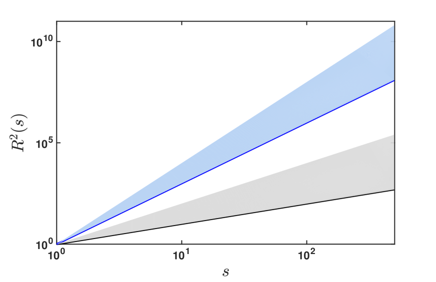
Figure 1: Scaling behaviour of the path MSD for stochastic processes discussed in this article. For the sake of simplicity we used a prefactor of $1$ in Eq. (7) for this figure, i.e. $R^{2}(s)=s^{2\alpha}$. The figure shows white noise with $\alpha=1/2$ (black line), fractional Gaussian noise with $1/2<\alpha<1$ (grey shaded area), Brownian motion with $\alpha=3/2$ (blue line) and fractional Brownian motion with $3/2<\alpha<1$ (blue shaded area). Note that we only consider specific values of the Hurst parameter $H$ here, see Eq. (8) for a detailed classification of the here discussed processes.

II.2.1 Increment represenation of the path MSD

In Eq. (6) the path MSD $R^{2}$ is defined as the squared displacement of the path. We also can express $R^{2}$ in relationhip with the autocovariance function

$$R^{2}(s)=\sum_{i,j=1}^{s}\text{Cov}(i,j)$$ (9)

which is derived by taking the square of the right hand side of Eq. (5). We call this equation the increment representation of the path MSD whereas its definition in Eq. (6) is called path representation. The increment representation is useful to understand the above discussed scaling of $R^{2}(s)$. For nonstationary FBM we refer to taqqu2 where the relationship $\alpha=H+1$ has been straigthforwardly calculated with the help of the right hand side of Eq. (9). For stationary processes it is possible to give a more intuitive understanding of the scaling behaviour of the path MSD and in particular why the path MSD or better an unbiased estimator of the path MSD is able to overcome the estimation problem (E1). First we order Eq. (9) according to the time lag $\tau$

$$R^{2}(s)=\sum_{i=1}^{s}\text{Cov}(0)+2\sum_{\tau=1}^{s-1}\sum_{i=1}^{s-\tau}\text{Cov}(\tau).$$ (10)

Since the autocovariance function $\langle\epsilon(i)\epsilon(i+\tau)\rangle$ doesn’t depend on the time point $i$ we can put the sum over $i$ to the right

$$R^{2}(s)=\text{Cov}(0)\left(s+2\sum_{\tau=1}^{s-1}C(\tau)(s-\tau)\right).$$ (11)

Inserting specific autocorrelation functions in this equation verifies the above explained scaling behaviour of $R^{2}(s)$ for stationary stochastic processes, see kantelhardt2 . We leave the detailed derivation out here since we present later a more general equation and verify the scaling there.

Finally with Eq. (11) we can understand why the path MSD overcomes the estimation problem (E1), see kantelhardt2 : The sum $\sum_{\tau=1}^{s-1}C(\tau)(s-\tau)$ in Eq. (11) scales in the same way as the integral $\int_{0}^{s}C(\tau)(s-\tau)\text{d}\tau$ which represents the area under $C(\tau)(s-\tau)$. Whereas the autocorrelation function decays in $s$, the integral increases, specifically with a power law decay $C(s)\sim s^{-\gamma}$ the integral scales like $s^{2-\gamma}$. Hence, the MSD overcomes (E1) because for large $s$ the values of also large, $s^{2-\gamma}$, and fluctuate only weakly in the log-log plot.

II.2.2 Estimation of the path MSD

We are in principle able to overcome the estimation problem (E1), but we have to find an estimator $\widehat{R^{2}}(s)$ of the path MSD $R^{2}(s)$ which can be applied to a given time series $\{x(t)\}_{t=1}^{N}$. This estimator should also be able to overcome estimation problem (E2). But this will be a difficult task which leads to a modified version of $\widehat{R^{2}}(s)$ and the introduction of detrending methods.

The increment representation of Eq. (9) directly connects the path MSD and the autocovariance function, namely by $R^{2}(s)=\sum_{i,j=1}^{s}\text{Cov}(i,j)$. We use this connection to connect similarly an estimator of the path MSD $\widehat{R^{2}}(s)$ to an estimator of the autocovariance function $\widehat{\text{Cov}}(i,j)$, namely by

$$\widehat{R^{2}}(s)=\sum_{i,j=1}^{s}\widehat{\text{Cov}}(i,j)$$ (12)

which is the increment represenation of the estimator of the path MSD. Below we will try to find a suitable estimator $\widehat{R^{2}}(s)$ in detail because this investigation serves as background of the motivation and formulation of detrending methods.

Although the autocovariance function is a function of the stochastic process $\{\epsilon(t)\}_{t=1}^{N}$, the estimator $\widehat{\text{Cov}}(i,j)$ is applied to the time series $\{x(t)\}_{t=1}^{N}$ and not the single realisation of the stochastic process. Possible external influences $\{m(t)\}_{t=1}^{N}$ are unknown a priori and might be part of the time series. Therefore we need to formulate an equivalent of the path for further investigation. The path is defined as the cumulative sum $r(t)=\sum_{i=1}^{t}\epsilon(i)$ of the stochastic process. Similarly we define the path of the time series as cumulative sum of the time series

$$y(t)=\sum_{i=1}^{t}x(i).$$ (13)

We also call this the profile. So the time series is understood as increment process of the profile. In the case of a pure random time series the profile is the path $y(t)=r(t)$. Similar to the path MSD $R^{2}=\langle r^{2}(s)\rangle$ we have now the profile MSD as $\langle y^{2}(s)\rangle$ which are identical again only for pure random time series.

III Pointwise averaging procedure

No matter if the time series is stationary or not, we simply use now the sample autocovariance function as estimator for the autocovariance function and study the consequences of our choice. The sample autocovariance function only depends on the time lag $\tau$ so we can use Eq. (11) and find $\widehat{R^{2}}(s)$ by replacing $\text{Cov}(\tau)$ with $\widehat{\text{Cov}}_{\text{sample}}(\tau)$, it follows

$$\widehat{R^{2}}_{\text{sample}}(s)=\widehat{\text{Cov}}_{\text{sample}}(0)s+2\sum_{\tau=1}^{s-1}\widehat{\text{Cov}}_{\text{sample}}(\tau)(s-\tau).$$ (14)

The notation "sample" as index of $\widehat{R^{2}}_{\text{sample}}(s)$ indicates the averaging procedure used for the estimation of the autocovariance function. If we use now the definition of the sample autocovariance function $\widehat{\text{Cov}}_{\text{sample}}(\tau)=1/(s-\tau)\sum_{i=1}^{s-\tau}x(i)x(i+\tau)$ then we find

$$\widehat{R^{2}}_{\text{sample}}(s)=\sum_{i,j=1}^{s}x(i)x(j).$$ (15)

but this is exactly the squared profile

$$\widehat{R^{2}}_{\text{sample}}(s)=y^{2}(s).$$ (16)

This result has two problems. First it does not estimate the path MSD but the profile MSD. Hence it will suffer from the unwanted influences of external nonstationarities. But this is expected since we simply used the sample autocovariance. Also the below introduced estimator will have problems with nonstationarity. The second and more obstructive problem of Eq. (16) is that the single value $y^{2}(s)$ is not a reliable estimate. Therefore we present in the next section a better estimation technique which is also used by detrending methods.

IV Segmentwise averaging procedure

IV.1 Segmentation of the time axis and estimator of the autocovariance function

In order to find a better estimator of the autocovariance function than in the previous subsection we have to replace the ensemble average in a suitable way. The meaning of the ensemble average of a random variable is that we ideally average over an infinite amount of samples. Therefore the autocovariance function can be understood as

$$\text{Cov}(i,j)=\langle\epsilon(i)\epsilon(j)\rangle=\lim_{K\to\infty}\frac{1}{K}\sum_{\nu=1}^{K}\epsilon^{(\nu)}(i)\epsilon^{(\nu)}(j).$$ (17)

Here $\{\epsilon^{(\nu)}(i)\}_{i\in\mathbb{N}}$ represents the $\nu$-th realisation of the stochastic process $\{\epsilon(i)\}_{i\in\mathbb{N}}$. In practice, the limit $K\to\infty$ cannot be performed, since we usually only have a finite sample, or as in this article, only one single realisation with finite length of the time axis. Given only one realisation $\{\epsilon^{(1)}(i)\}_{i=1}^{N}$ we replace the ensembles in Eq. (17) appropriately using a segmentation of the time axis which is done as follows.

We divide the time axis $[1,N]$ into $K\in\mathbb{N}$ segments of length $s$. The $\nu$-th segment consists of the time points $[1+d_{v},s+d_{v}]$ with $\nu\in\{1,K\}$. The quantity $d_{v}$ shifts time points from the first to the $\nu$-th segment

$$i\in[1,s]\Rightarrow i+d_{v}\in[1+d_{v},s+d_{v}]$$ (18)

and we therefore call $d_{\nu}$ shift factor which also depends on $s$. For the first segment $\nu=1$ we claim $d_{1}=0$. For the last segment $\nu=K$ the inequality has to be hold $s+d_{K}\leq N$. Note that such a segmentation of the time axis $[1,N]$ usually has some leftovers which are not in any of the segments $[1+d_{\nu},s+d_{\nu}]$. For the sake of simplicity we don’t treat them here. Time points can be shifted from the first segment to the $\nu$-th one in many possible ways depending on the exact form of the shift factor $d_{\nu}$. We discuss now two important ones. First the segments can be shifted subsequently so that we have the segments

$$[1,s],[2,s+1],[3,s+2],\ldots,[1+d_{K},s+d_{K}].$$ (19)

Here the shift factor is $d_{\nu}=\nu-1$ and we have $K=N-s+1$ segments. Alternatively, the segments can be shifted with distance $s$ such that we have the disjoint segments

$$[1,s],[s+1,2s],[2s+1,3s],\ldots,[1+d_{K},s+d_{K}].$$ (20)

Here the shift factor is $d_{\nu}=(\nu-1)s$ and we have $K=\lfloor N/s\rfloor$ segments with the floor function $\lfloor\ldots\rfloor$. Both shifting procedures are later used in this article.

This segmentation of the time axis helps us to estimate the autocovariance function of Eq. (17) when only one realisation $\{\epsilon^{(1)}(i)\}_{i=1}^{N}$ is given as it is often the case in time series analysis. We cut this realisation into segments and take these as ensemble

$$\{\epsilon^{(1)}(i+d_{\nu})\}_{i=1}^{s}\longleftrightarrow\{\epsilon^{(\nu)}(i)\}_{i=1}^{s},$$ (21)

see figure 2. For the sake of simplicity we skip the symbol the first realisation $(1)$ in the following $\epsilon^{(1)}(i)\rightarrow\epsilon(i)$ and hence go back to our previous notation. We can now define an estimator of the autocorrelation function by using the replacement of Eq. (21) for the autocovariance function of Eq. (17) for finite $K$, namely

$$\widehat{\text{Cov}}_{\text{seg}}(i,j)=\frac{1}{K}\sum_{\nu=1}^{K}\epsilon(i+d_{\nu})\epsilon(j+d_{\nu}).$$ (22)

The index "seg" stands for segment. This estimator is only unbiased for stationary stochastic processes $\langle\widehat{\text{Cov}}_{\text{seg}}(i,j)\rangle=\text{Cov}(i,j)$ but not for nonstationary processes. But this is not suprising because the replacement of ensembles with the realisation in segments is only reasonable for stationarity. Nevertheless the here introduced segmentwise estimator of the autocovariance function will play an important role in detrending methods and we will therefore continue to investigate it.

Due to construction this estimator is applied to a pure random time series $x(t)=\epsilon(t)$ which is of course unknown a priori. An actual practical estimator is applied on the full time series and we therefore can finally define the segmentwise averaging estimator of the autocovariance function as

$$\widehat{\text{Cov}}_{\text{seg}}(i,j)=\frac{1}{K}\sum_{\nu=1}^{K}x(i+d_{\nu})x(j+d_{\nu}).$$ (23)

This estimator implies that the the $\nu$-th segment of the single given time series represents the $\nu$-th realisation of an assumed existing ensemble of time series. Using this result we will find next an estimator of the path MSD.

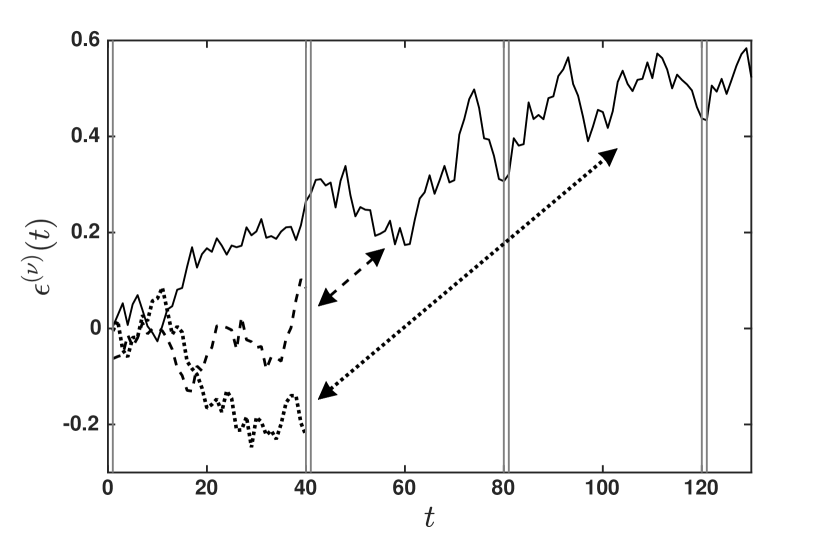
Figure 2: Schematic representation of the of the replacement of the $\nu$-th realisation in the first segment $\{\epsilon^{(\nu)}(i)\}_{i=1}^{s}$ by the first realisation in the $\nu$-th segment $\{\epsilon^{(1)}(i)\}_{i=1+d_{\nu}}^{s+d_{\nu}}$ with $\nu\in\{1,K\}$, see Eq. (21). It is shown here for $K=3$ realisations/segments with Brownian motion as stochastic process. The first realisation (solid line) represents the time series, the second (dashed line) and third realisation (dotted line) are assumed to exist theoretically in the first segment, see more details in the text of this section. Here the segments have a length of $s=40$ and are disjoint with shift factor $d_{\nu}=(\nu-1)s$.

IV.2 Estimator of the path MSD

Now we take the relationship between the path MSD and the autocovariance function $R^{2}(s)=\sum_{i,j=1}^{s}\text{Cov}(i,j)$ of Eq. (9) and replace the autocovariance function with the segmentwise averaging estimator of Eq. (23). So we obtain the estimator of the path MSD as

$$\begin{split}\widehat{R^{2}}_{\text{seg}}(s)&=\sum_{i,j=1}^{s}\widehat{\text{Cov}}_{\text{seg}}(i,j)\\ &=\frac{1}{K}\sum_{\nu=1}^{K}\sum_{i,j=1}^{s}x(i+d_{\nu})x(j+d_{\nu}).\end{split}$$ (24)

In the second step we put the sum over the segments to the left. The notation "seg" as index of $\widehat{R^{2}}_{\text{seg}}(s)$ indicates the segmentwise averaging procedure used for the estimation of the autocovariance function. This equation is the increment representation of the estimator $\widehat{R^{2}}_{\text{seg}}(s)$. The path representation can be derived with respect to the profile of the time series. The double sum of the time series over $i$ and $j$ in Eq. (24) can be written as the squared sum of the time series

$$\sum_{i,j=1}^{s}x(i+d_{\nu})x(j+d_{\nu})=\left(\sum_{i=1}^{s}x(i+d_{\nu})\right)^{2}.$$ (25)

Inside this square the sum of the time series is equivalent to the profile displacement

$$\sum_{i=1}^{s}x(i+d_{\nu})=\sum_{i=1}^{s+d_{\nu}}x(i)-\sum_{i=1}^{d_{\nu}}x(i)=y(s+d_{\nu})-y(d_{\nu}),$$ (26)

see figure 3. So the sum of the time series over all points in the segment $\nu$ of length $s$ is the same as the displacement of the profile where the profile starts at $t=d_{\nu}$ and walks a time interval of $s$ until $t=s+d_{\nu}$. Using this connection we can write the estimator $\widehat{R^{2}}_{\text{seg}}(s)$ in Eq. (24) as average of the squared displacements of the profile

$$\widehat{R^{2}}_{\text{seg}}(s)=\frac{1}{K}\sum_{\nu=1}^{K}(y(s+d_{\nu})-y(d_{\nu}))^{2}$$ (27)

where we average over the number of segments. We call this equation the path representation of the estimator.

The estimator of the path MSD is a general form of two well-known quantities depending on the shift factor $d_{\nu}$. For the subsequent shift factor $d_{\nu}=\nu-1$ the estimator $\widehat{R^{2}}_{\text{seg}}(s)$ is the time averaged mean squared displacement (TAMSD) of the profile

$$\widehat{R^{2}}_{\text{seg}}(s)=\frac{1}{K}\sum_{\nu=0}^{K-1}(y(s+\nu)-y(\nu))^{2}$$ (28)

with $K=N-s+1$ where we decremented the summation index $\nu$ by $1$. Note that $y(0)=0$. A modification of this estimator will later lead to the method of detrending moving average. In the other case described above, the disjoint segmentation with shift factor $d_{\nu}=(\nu-1)s$ the estimator $\widehat{R^{2}}_{\text{seg}}(s)$ is the fluctuation function of the method of fluctuation analysis

$$\widehat{R^{2}}_{\text{seg}}(s)=\frac{1}{K}\sum_{\nu=0}^{K-1}(y((\nu+1)s)-y(\nu s))^{2}$$ (29)

with $K=\lfloor N/s\rfloor$, see kantelhardt2 . Here we also decremented the summation index $\nu$ by $1$. A modification of this fluctuation function with the help of Eq. (24) will later lead to the method of detrended fluctuation analysis.

Summarized, the here introduced estimator $\widehat{R^{2}}_{\text{seg}}(s)$ allows later a simple modification which leads to the basic principle of detrending of detrending methods. This modification is applied to $\widehat{R^{2}}_{\text{seg}}(s)$ in the increment representation of Eq. (24). A modification with the help of the path representation of Eq. (27) is not always possible, e.g., not to derive detrended fluctuation analysis DFA.

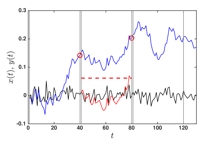
Figure 3: Schematic representation of the equivalence between the profile displacement $y(s+d_{\nu})-y(d_{\nu})$ and the cumulative sum of the time series $\sum_{i=1}^{s}x(i+d_{\nu})$, see Eq. (26). We used white noise (black line)/Brownian motion (blue line) as time series/profile and disjoint segments of length of $s=40$ with the shift factor $d_{\nu}=(\nu-1)s$. The figure highlights the relationship in the second segment $\nu=2$ where we display the time series $\{\sum_{i=1}^{t}x(i+d_{2})\}_{t=1}^{s}$ (red line) and the two points of the profile $y(d_{2})$ and $y(s+d_{2})$ (two red dots). The relationship of Eq. (26) says that $\sum_{i=1}^{s}x(i+d_{2})$ and $y(s+d_{2})-y(d_{2})$ are equivalent which is indicated with the red dashed line in this figure.

IV.3 Bias of the estimator of the path MSD

The bias of the estimator $\widehat{R^{2}}_{\text{seg}}(s)$ is given by the difference between the mean of the estimator of the path MSD and the path MSD

$$B(s)=\langle\widehat{R^{2}}(s)\rangle-R^{2}(s).$$ (30)

In order to derive the bias in the case of the segmentwise averaging procedure we need to calculate the mean of the estimator $\widehat{R^{2}}_{\text{seg}}(s)$ for which we use the increment representation

$$\langle\widehat{R^{2}}_{\text{seg}}(s)\rangle=\frac{1}{K}\sum_{\nu=1}^{K}\sum_{i,j=1}^{s}\langle x(i+\delta_{\nu})x(j+\delta_{\nu})\rangle.$$ (31)

Below we will analyze $\langle\widehat{R^{2}}_{\text{seg}}(s)\rangle$ depending on the stationarity of the time series. We will see that the estimator is only unbiased for stationary processes but not for nonstationary ones.

IV.4 Stationary time series

Here we analyze the bias of the estimator $\widehat{R^{2}}_{\text{seg}}(s)$ for stationary time series. When the time series is stationary, then our model is a pure random time series $x(t)=\epsilon(t)$ because there can be no additive trends $m(t)=0$.

Using the increment representation of Eq. (31) we find for the mean of the estimator

$$\langle\widehat{R^{2}}_{\text{seg}}(s)\rangle=\sum_{i,j=1}^{s}\text{Cov}(i,j)$$ (32)

which is exactly the path MSD $R^{2}(s)$. We used that the stationary autocovariance function is independent of the segment $\langle\epsilon(i+\delta_{\nu})\epsilon(j+\delta_{\nu})\rangle=\langle\epsilon(i)\epsilon(j)\rangle$. So the estimator is unbiased

$$\langle\widehat{R^{2}}_{\text{seg}}(s)\rangle=R^{2}(s).$$ (33)

The same result can be obtained with the path representation

$$\langle\widehat{R^{2}}_{\text{seg}}(s)\rangle=\frac{1}{K}\sum_{\nu=1}^{K}\langle(r(s+d_{\nu})-r(d_{\nu}))^{2}\rangle=\langle r^{2}(s)\rangle$$ (34)

which is also the path MSD. We used that the displacements of the path are stationary.

In summary, the estimator $\widehat{R^{2}}_{\text{seg}}(s)$ estimates the path MSD in the case of a pure random and stationary time series. Furthermore this estimator is unbiased. As estimator with an increasing scaling behaviour it overcomes the estimation problem (E1) from section II.1. Below we will see that nonstationarity and therefore the estimation problem (E2) is still a problem.

IV.5 Nonstationary time series

In the following two subsections we calculate $\langle\widehat{R^{2}}_{\text{seg}}(s)\rangle$ for two different types of nonstationarity and study the bias of the estimator. We have to analyze the autocovariance function of the time series in the $\nu$-th segment $\langle x(i+d_{\nu})x(j+d_{\nu})\rangle$ of the increment representation in Eq. (31). In the path representation of Eq. (27) it is immediately clear that the estimator fails because it is averaged over nonstationary displacements. Nevertheless we analyze $\langle\widehat{R^{2}}_{\text{seg}}(s)\rangle$ in the increment representation because first it shows clearly why this estimator fails and second it allows modification to overcome the problem of nonstationarity.

IV.5.1 Intrinsic nonstationarity

If a time series is represented by a nonstationary stochastic process without additional trends then this nonstationarity is called intrinsic, see hoell3 . As example we investigate Brownian motion and show that the estimator $\widehat{R^{2}}_{\text{seg}}(s)$ is biased.

In order to calculate the mean of the estimator of Eq. (31) we need first to calculate the autocovariance function of the time series in the $\nu$-th segment $\langle x(i+d_{\nu})x(j+d_{\nu})\rangle$ which is here identical to the autocovariance function of Brownian motion in the $\nu$-th segment $\langle\epsilon(i+d_{\nu})\epsilon(j+d_{\nu})\rangle$. The autocovariance function can be split into two parts

$$\begin{split}\langle\epsilon(i+d_{\nu})\epsilon(j+d_{\nu})\rangle&=\text{min}(i+d_{\nu},j+d_{\nu})\\ &=\text{Cov}(i,j)+d_{\nu}\end{split}$$ (35)

with $\text{Cov}(i,j)=\text{min}(i,j)$. Hence the autocovariance function in $\nu$-th segment is the autocovariance function of the first segment plus the shift factor. Interestingly, the dependence of the segment $\nu$ is fully described by the second part, see figure 4. This splitting of the autocovariance function leads also to a splitting of the mean of the estimator in Eq. (31), namely

$$\langle\widehat{R^{2}}_{\text{seg}}(s)\rangle=\sum_{i,j=1}^{K}\text{Cov}(i,j)+\frac{1}{K}\sum_{\nu=1}^{K}\sum_{i,j=1}^{s}d_{\nu}$$ (36)

where the segment average $1/K\sum_{\nu=1}^{K}$ gives $1$ for the first part on the right hand side because $\text{Cov}(i,j)$ is independent of the segment $\nu$. This first part is exactly the path MSD $R^{2}(s)$. Therefore the second part is the bias of the estimator

$$B(s)=\frac{1}{K}\sum_{\nu=1}^{K}\sum_{i,j=1}^{s}d_{\nu}.$$ (37)

So the estimator $\widehat{R^{2}}_{\text{seg}}(s)$ is biased. And the bias is the reason why the estimator $\widehat{R^{2}}_{\text{seg}}(s)$ cannot detect the scaling of the path. This can be shown by calculating $R^{2}(s)$ and $B^{2}(s)$ explicitely. The path MSD is calculated as

$$R^{2}(s)=\frac{1}{3}s^{3}+\frac{1}{2}s^{2}+\frac{1}{6}s$$ (38)

which scales cubically

$$R^{2}(s)\sim\frac{1}{3}s^{3}$$ (39)

for large $s$ and therefore gives a fluctuation parameter $\alpha=3/2$ as discussed in section II.2. The bias $B(s)$ can be calculated for subseguent shifting of the segments with the shift factor $d_{\nu}=v-1$ and $K=N-s+1$ segments and also for disjoint shifting with the shift factor $d_{\nu}=(\nu-1)s$ and $K=N/s$ segments. Note that we use $K=N/s$ and not $K=\lfloor N/s\rfloor$ for the sake of simplicity. In both cases we obtain

$$B(s)=-\frac{1}{2}s^{3}+\frac{N}{2}s^{2}.$$ (40)

The segment length $s$ cannot be larger than the time axis $N$. Even more, the segmentwise averaging procedure requires enough segments $K$ in order to obtain a reliable estimation of the autocovariance function. This requirement reduces the largest possible value of $s$ to some value smaller than $N$. For those allowed values of $s$ the scaling of the bias $B(s)$ dominated by the quadratic term

$$B(s)\sim\frac{N}{2}s^{2}$$ (41)

because the prefactor of the quadtratic term, $N/2$, is bigger than $s$ and hence $\frac{N}{2}s^{2}>\frac{1}{2}s^{3}$. And since $\langle\widehat{R^{2}}_{\text{seg}}(s)\rangle$ is the sum of $R^{2}$ and $B^{2}$ we obtain quadratic scaling of the mean of the estimator

$$\langle\widehat{R^{2}}_{\text{seg}}(s)\rangle\sim\frac{N+1}{2}s^{2}$$ (42)

with the same argument as for the scaling of $B^{2}$. This means that the estimator estimator $\widehat{R^{2}}_{\text{seg}}(s)$ applied on a time series which is a single realisation of Brownian motion estimates a fluctuation parameter of

$$\hat{\alpha}=1.$$ (43)

Here $\hat{\alpha}$ is the estimated slope of $\widehat{R^{2}}_{\text{seg}}(s)$ in the log-log plot which can be observed after applying the estimator $\widehat{R^{2}}_{\text{seg}}(s)$ on a single realisation of Brownian motion. This estimated fluctuation parameter $\hat{\alpha}=1$ is a known result for the method of fluctuation analysis hoell3 and obviously a flaw of this method. In fact it is a wrong estimation because for Brownian motion the fluctuation parameter is $\alpha=3/2$. The reason for this wrong scaling comes from the bias $B^{2}(s)$ which dominates the scaling of the estimator. In addition, we also observe numerically the same scaling $\hat{\alpha}=1$ for FBM with $1/2<H<1$ and assume similar behaviour of the bias. In summary, in the case of a pure random and nonstationary time series as in the case of BM or FBM the estimator of the path MSD using segmentwise averaging procedure has a different scaling than the path MSD.

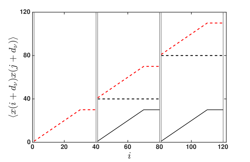
Figure 4: Splitting of the autocovariance function in the $\nu$-th segment $\langle x(i+d_{\nu})x(j+d_{\nu})\rangle=\langle\epsilon(i+d_{\nu})\epsilon(j+d_{\nu})\rangle$ (dashed red line) of Brownian motion into the autocovariance function of the first segment $\text{Cov}(i,j)$ (solid black line) and the autocovariance difference $d_{\nu}$ (dashed black line), see Eq. (35). Here it is $j=30$. And the segments have a length of $s=40$ and are disjoint with shift factor $d_{\nu}=(\nu-1)s$.

IV.5.2 External nonstationarity

Here we calculate $\langle\widehat{R^{2}}_{\text{seg}}(s)\rangle$ for a time series with an external nonstationarity. We model this by a stationary stochastic process $\epsilon(t)$ with an additional deterministic trend, see hoell3 . As example we investigate white noise added to a linear trend,

$$x(t)=\epsilon(t)+mt$$ (44)

and show that the estimator $\widehat{R^{2}}_{\text{seg}}(s)$ is biased. The autocovariance function of the time series in the $\nu$-th segment can again be split into two parts

$$\langle x(i+d_{\nu})x(j+d_{\nu})\rangle=\text{Cov}(i,j)+(i+d_{\nu})(j+d_{\nu})$$ (45)

with the autocovariance function of white noise $\text{Cov}(i,j)=1$ for $i=j$ and $0$ for $i\neq j$. The second part on the right hand side comes from the linear trend. This part completely governs the dependence of the segments. A similar splitting of $\langle x(i+d_{\nu})x(j+d_{\nu})\rangle$ has also been found for the intrinsic nonstationarity of Brownian motion where the first part is the autocovariance function in the first segment and the second part describes the dependence of the segments. The following discussion will therefore be similar to the Brownian motion case.

The splitting of the autocovariance function of Eq. (45) leads also to a splitting of the mean of estimator in Eq. (31), namely

$$\langle\widehat{R^{2}}_{\text{seg}}(s)\rangle=\sum_{i,j=1}^{s}\text{Cov}(i,j)+\frac{m^{2}}{K}\sum_{\nu=1}^{K}\sum_{i,j=1}^{s}(i+d_{\nu})(j+d_{\nu}).$$ (46)

Again the first part is the path MSD and therefore the second part is the bias of the estimator

$$B(s)=\frac{m^{2}}{K}\sum_{\nu=1}^{K}\sum_{i,j=1}^{s}(i+d_{\nu})(j+d_{\nu}).$$ (47)

So the estimator is biased. The path MSD of white noise is given by

$$R^{2}(s)=s$$ (48)

and therefore gives a fluctuation parameter $\alpha=1/2$ as discussed in section II.2. The full solution of the bias $B(s)$ depends on the segmentation. For subsequent segmentation the bias is

$$B(s)=m^{2}\left(\frac{1}{12}s^{4}-\frac{N+1}{6}s^{3}+\frac{4N^{2}+8N+3}{12}s^{2}\right)$$ (49)

and for disjoint segmentation the bias is

$$B(s)=-\frac{m^{2}}{12}s^{4}+\frac{4N^{2}+6N+3}{12}m^{2}s^{2}.$$ (50)

Nevertheless for allowed values of $s$ as explained for Brownian motion both solutions are approximately similar. The bias scales quadratically

$$B(s)\sim\frac{N^{2}m^{2}}{3}s^{2}$$ (51)

because of the largest prefactor $N^{2}/3$. And since $\langle\widehat{R^{2}}_{\text{seg}}(s)\rangle$ is the sum of $R^{2}$ and $B$ we obtain quadratic scaling of the mean of the estimator

$$\langle\widehat{R^{2}}_{\text{seg}}(s)\rangle\sim\frac{N^{2}m^{2}}{3}s^{2}$$ (52)

with the same argument as for the bias. This means that the estimator $\widehat{R^{2}}_{\text{seg}}(s)$ applied to a time series which is a composition of white noise and a linear trend asymtotically estimates a fluctuation parameter of

$$\hat{\alpha}=1.$$ (53)

So the estimator is not able to detect the fluctuation parameter $\alpha=1/2$ of white noise. Numerical tests also show $\hat{\alpha}=1$ where we use FGN with $\alpha=H$ and $1/2<H<1$ instead of white noise. And we obtain also $\hat{\alpha}=1$ when we use trends of higher order in $t$ instead of linear. The bias which comes here only from the additive trend dominates the scaling of the estimator and destroys information about the stationary stochastic process. This wrong scaling of $\hat{\alpha}=1$ is well-known for the method of fluctuation analysis as it can be seen in kantelhardt2 but has not yet been explained by the influence of the bias on the scaling behaviour.

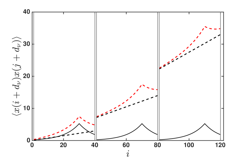
Figure 5: Splitting of the autocovariance function in the $\nu$-th segment $\langle x(i+d_{\nu})x(j+d_{\nu})\rangle$ (dashed red line) of an AR($1$) process with additive linear trend with slope $0.05$ into the autocovariance function of the first segment of the AR($1$) process $\text{Cov}(i,j)$ (solid black line) and the autocovariance difference $0.05^{2}(i+d_{\nu})(j+d_{\nu})$ (dashed black line), see Eq. (45). The AR($1$) process has the autocorrelation function $C(|i-j|)=0.9^{|i-j|}$. Here it is $j=30$. And the segments have a length of $s=40$ and are disjoint with shift factor $d_{\nu}=(\nu-1)s$. Note that we use white noise instead of an AR($1$) process in the text of this section. But the situation of the splitting of the autocovariance function remains.

IV.5.3 Summary

In the previous subsections we have seen that the estimator $\widehat{R^{2}}_{\text{seg}}(s)$ yields an estimation of the scaling exponent of $\widehat{\alpha}=1$ in the case of nonstationarity no matter what stochastic process is underlying the time series. The estimator is neither able to detect the fluctuation parameter $\alpha$ of the path for intrinsic nor for external nonstationary time series. Here we summarize these results, which are the motivation for detrending methods in the next section.

The mean of the estimator $\langle\widehat{R^{2}}_{\text{seg}}(s)\rangle$ depends on the autocovariance function of the time series in the $\nu$-th segment. For intrinsic and external nonstationarity this can be split into the autocovariance function of the stochastic process in the first segment and a segment-dependent part

$$\langle x(i+d_{\nu})x(j+d_{\nu})\rangle=\text{Cov}(i,j)+D_{\nu}(i,j).$$ (54)

We call from now $D_{\nu}(i,j)$ the autocovariance difference of the time series $x(t)$. This splitting leads to a splitting of the mean of the estimator

$$\langle\widehat{R^{2}}_{\text{seg}}(s)\rangle=R^{2}(s)+B(s),$$ (55)

namely into the path MSD and the bias

$$B(s)=\frac{1}{K}\sum_{\nu=1}^{K}\sum_{i,j=1}^{s}D_{\nu}(i,j).$$ (56)

The bias can be seen as the estimator applied to the autocovariance differences. Due to the limitation $s<N$, the bias itself is dominated by one summand which scales like $s^{2}$, which then dominates the scaling of the mean of the estimator

$$\langle\widehat{R^{2}}_{\text{seg}}(s)\rangle\sim B(s)\sim s^{2}\;.$$ (57)

This leads to an estimation of the fluctuation parameter of $\widehat{\alpha}=1$ for a given time series no matter what stochastic process is realised in this time series.

In contrast, for stationary time series the autocovariance differences are zero and so is the bias. In that case the estimator is unbiased. We will provide in the following an estimator for the path MSD which is unbiased also in the case of nonstationarity which is therefore a solution to the estimation problem (E2) of section II.1.

V Detrending methods

V.1 Motivation

Given a time series we want to estimate the scaling behaviour of the path MSD of its stochastic component. For this task the estimator $\widehat{R^{2}}_{\text{seg}}(s)$ is unsuitable due to its failure for nonstationary time series. This can be easily understood in its path representation $\widehat{R^{2}}_{\text{seg}}(s)=1/K\sum_{\nu=1}^{K}(y(s+d_{\nu})-y(d_{\nu}))^{2}$ because the displacements $y(s+d_{\nu})-y(d_{\nu})$ are nonstationary. But we used the increment representation $\widehat{R^{2}}_{\text{seg}}(s)=1/K\sum_{\nu=1}^{K}\sum_{i,j=1}^{s}x(i+d_{\nu})x(j+d_{\nu})$ of the estimator to show in detail the origin of a bias and how this bias destroys the asymptotic scaling. To overcome this problem we introduce here a bunch of new quantities which are all analogue to the already investigated ones. Those new quantities are the foundation of detrending methods.

V.2 The fluctuation function

For the following we want to recall that the path was defined as the cumulative sum of the stochastic process $r(t)=\sum_{i=1}^{t}\epsilon(i).$ Everything what follows now is based on the replacement of the squared path displacement in the increment representation $(r(s)-r(0))^{2}=\sum_{i,j=1}^{s}\epsilon(i)\epsilon(j)$ with the so-called generalised squared path displacement

$$f^{2}(s)=\sum_{i,j=1}^{s}\epsilon(i)\epsilon(j)L(i,j,s)$$ (58)

which is weighted in the increment representation with the weights $L(i,j,s)$. The purpose of the weights $L(i,j,s)$ is to suppress the effects of external nonstationarity and to guarantee the correct scaling with $\alpha>1$ for intrinsic nonstationarities. The next important new quantity is a generalistation of the path MSD. The path MSD was defined as the mean of the squared path displacement $R^{2}=\langle(r(s)-r(0))^{2}\rangle$. We now define the fluctuation function as mean of the generalised squared path displacement

$$F^{2}(s)=\langle f^{2}(s)\rangle.$$ (59)

Using the definition of the generalised squared path displacement the fluctuation function reads

$$F^{2}(s)=\sum_{i,j=1}^{s}\text{Cov}(i,j)L(i,j,s).$$ (60)

for which $R^{2}(s)=\sum_{i,j=1}^{s}\text{Cov}(i,j)$ of Eq. (9) is the analogue equation of the path MSD.

V.3 Estimator of the fluctuation function

We introduce the estimator of the fluctuation function

$$\begin{split}\widehat{F^{2}}(s)&=\sum_{i,j=1}^{s}\widehat{\text{Cov}}_{\text{seg}}(i,j)L(i,j,s)\\ &=\frac{1}{K}\sum_{\nu=1}^{K}\sum_{i,j=1}^{s}x(i+d_{\nu})x(j+d_{\nu})L(i,j,s)\end{split}$$ (61)

which is similarly constructed as $\widehat{R}^{2}_{\text{seg}}(s)$ of Eq. (24). This means we have replaced the autocovariance function in Eq. (60) by the segmentwise averaging estimator of the autocovariance function. Eq. (61) implies that the generalised squared path displacement $f$ is estimated in the $\nu$-th segment by

$$f_{\nu}^{2}(s)=\sum_{i,j=1}^{s}x(i+d_{\nu})x(j+d_{\nu})L(i,j,s)$$ (62)

which is analogue to the squared profile displacement in the increment representation $(y(s+d_{\nu})-y(d_{\nu}))^{2}=\sum_{i,j=1}^{s}x(i+d_{\nu})x(j+d_{\nu})$. Hence the estimator of the fluctuation function can also be understood as average of these estimators of the generalised squared path displacements

$$\widehat{F^{2}}(s)=\frac{1}{K}\sum_{\nu=1}^{K}f^{2}_{\nu}(s)$$ (63)

averaged over all segments. This equation can be seen as the path representation of the estimator. We should note that in the existing literature the term "fluctuation function" is used for the estimator of the fluctuation function. But in our framework we need to be more careful with the concepts.

V.4 Basic principles of detrending methods

A detrending method provides a way to specify weights $L(i,j,s)$ such that the fluctuation function respectively its estimator fulfil the following two principles:

• Scaling: The fluctuation function should have the same asymptotic scaling behaviour as the path MSD

  $$F^{2}(s)\sim s^{2\alpha}$$ (64)

  with the fluctuation parameter $\alpha$.

• Unbiasedness: The estimator of the fluctuation function should be unbiased

  $$\langle\widehat{F^{2}}(s)\rangle=F^{2}(s).$$ (65)

The principles (L1) and (L2) solve the estimation problems (E1) and (E2). The first principle (L1) means that the fluctuation function scales increasingly with two times the fluctuation parameter $\alpha$. So the weights should have no influence on the scaling behaviour compared to the path MSD. With such an increasing power law the estimation problem (E1) is overcome. Of course the same scaling should be exhibited by the estimator which is governed by the second principle. Taking the mean of the estimator $\langle\widehat{F^{2}}(s)\rangle$ in Eq. (61) creates the autocovariance function $\langle x(i+d_{\nu})x(j+d_{\nu})\rangle$. For the above explained types of nonstationarity it splits into the autocovariance function $\text{Cov}(i,j)$ and the autocovariance differences $D_{\nu}(i,j)$. The second principle which requires a bias of zero then leads to

$$B(s)=\frac{1}{K}\sum_{\nu=1}^{K}\sum_{i,j=1}^{s}D_{\nu}(i,j)L(i,j,s)=0.$$ (66)

This equation is the mathematical formulation of what detrending should achieve. In the literature, detrending is used to describe methods which, by removing non-stationarities from (parts of) the time series $x(t)$, restore the correct scaling. In our formalism, detrending means that the differences of the autocovariance function between segments has no influence on the estimation of the fluctuation function. In addition, for stationary processes (L2) holds trivially because the autocovariance differences are zero $D_{\nu}(i,j)=0$. So the second principle (L2) indeed overcomes the estimation problem (E2).

Unfortunately it is not easy to find appropriate weights $L(i,j,s)$. But luckily there exist already methods such as detrended fluctuation analysis and detrending moving average which serve as possible candidates for being examples of detrending methods. But their estimators of the fluctuation function are not in the form of Eq. (61) and it is some effort necessary to show the equivalence.

V.5 Practical implementation

Let us assume we know the specific form of the weights $L(i,j,s)$. Given a time series $x(t)_{t=1}^{N}$ the implementation of detrending methods consists of three steps:

• We divide the time axis into $K$ segments of length $s$ with the $\nu$-th segment given by $[1+d_{\nu},s+d_{\nu}]$.

• In every segment we calculate the estimator of the generalised squared profile displacements $f_{\nu}^{2}(s)$.

• We average $f^{2}_{\nu}(s)$ over all segments and obtain the estimator of the fluctuation function $\widehat{F^{2}}(s)$.

All three steps are repeated for different values of the segment length $s$. Because of the scaling behaviour

$$\widehat{F^{2}}(s)\sim s^{2\widehat{\alpha}}.$$ (67)

we find an estimation of the fluctuation parameter $\widehat{\alpha}$ by linear fitting in the log-log plot.

V.6 Detrending procedure

The detrending procedure is the centerpiece of detrending methods. And since we provided a new and general framework we want to summarize what we now understand under detrending. The following three descriptions are used equivalently:

• When a time series is successfully detrended in the framework of detrending methods then the estimator of the fluctuation function scales asymptotically as the path MSD. Hence we can observe the fluctuation parameter $\alpha$ of the stochastic process underlying the time series.

• The principle (L2) holds which means that the estimator of the fluctuation function is unbiased. This implies a zero bias $B(s)=0$ which is the case when the autocovariance differences between segments $D_{\nu}(i,j)$ have no influence on the estimation procedure.

• The estimators of the generalised squared path displacements $f_{\nu}^{2}(s)$ are identically distributed with respect to the segments. Then the average of $f_{\nu}^{2}(s)$ over all segments provides a unbiased estimation of the fluctuation function.

Description (A) is what is usually understood as detrending in the literature. For instance, the fluctuation parameter $\alpha$ of the DFA fluctuation function for FBM has been analytically derived in movahed . There the original description of the fluctuation function which is not the increment representation has been used. Hence this derivation is unaware of the unbiasedness of the estimator of the fluctuation function which is exactly stated in description (B) and which is firstly described here in this article. Description (C) has been has already been used in hoell3 for DFA applied on FBM. There it has been pointed out that the statistical equivalence of the estimator of the generalised squared path displacements

$$\langle f_{\nu}^{2}(s)\rangle=\langle f_{\omega}^{2}(s)\rangle$$ (68)

for all segments $\nu$ and $\omega$ is necessary in order to satisfy the first principle (L1) of detrending methods. There the unbiasedness of the estimator of the fluctuation function was not mentioned explicitily. But in the here presented framework Eq. (68) is exactly the second principle (L2).

V.7 Superposition principle

The case of external nonstationarity served as motivation to establish detrending methods. It consists of a stationary stochastic process and a deterministic trend. Actually this is a special case of two general processes. If the time series is a composition of two processes $x(t)=x_{1}(t)+x_{2}(t)$ and both are independent of each other then the fluctuation function is the sum of two single ones

$$F^{2}(s)=F_{1}^{2}(s)+F_{2}^{2}(s)$$ (69)

where $F^{2}_{n}(s)$ is the fluctuation function of the process $\{x_{n}(t)\}_{t=1}^{N}$ with $n=1$ and $2$, see hu . This is the superposition principle. Independence between both single processes implies zero cross-correlation $\langle x_{1}(i)x_{2}(j)\rangle=0$ for all $i$ and $j$. Using this in Eq. (60) gives the superposition principle of the fluctuation function. When the second principle (L2) holds then the superposition principle also holds for the estimators of the fluctuation functions.

As special case of external nonstationarity, when the first process is a stationary stochastic process and the second process is a deterministic trend then the superposition principle yields that $F_{1}^{2}(s)$ is the full fluctuation function and $F_{2}^{2}(s)$ is the bias which should be zero under successfull detrending.

V.8 Factorisable weights and wavelets

If the weights are factorisable

$$L(i,j,s)=l(i,s)l(j,s)$$ (70)

then the estimator of the generalised path displacement can be written as weighted sum of the time series

$$f_{\nu}(s)=\sum_{i=1}^{s}x(i+d_{\nu})l(i,s)$$ (71)

with weights $l(i,s)$. This equation is a generalisation of the relationship between the profile displacement and the time series as $y(s+d_{\nu})-y(d_{\nu})=\sum_{i=1}^{s}x(i+d_{\nu})$. As we will see later the method of detrending moving average DMA has factorisable weights, but detrended fluctuation analysis DFA does not.

Another popular estimation method for the scaling exponent with build-in detrending relies on a wavelet transform abry ; veitch . The quantity which corresponds to the fluctuation function Eq. (60) is there the time average of the squared scale-$s$ wavelet coefficient, averaged over all disjoint windows of length $s$ contained in the time series. Its scaling exponent $\beta$ is related to the exponent $\alpha$ used here by $\beta=2\alpha-1$. The detrending is here achieved by choosing wavelets whose first $n$ moments vanish, so that power law trends up to order $n-1$ are projected out from the wavelet transform. The method becomes particularly simple if wavelets are taken from the famility of Haar wavelets abry . The wavelet method therefore is a variant of Eq. (71), where the wavelet is a special choice of the kernel $l(i,s)$, see also kiyono5 .

VI DFA and DMA

In previous section, we introduced basic principles of detrending methods. Now we will show that detrended fluctuation analysis (DFA) and detrending moving average (DMA) are examples of such methods. In order to do so we need to answer two questions: How can we come from the original form of the estimator of the fluctuation function of DFA and DMA to the here introduced one in the increment representation? And what are the specific expressions of the weights $L(i,j,s)$ for DFA and DMA? Both methods are constructed differently nevertheless we present them simultaneously in the following to emphasize their similarities and differences. We then show the ability of DFA and DMA to fulfill basic principles (L1) and (L2).

VI.1 Original description

We present here the original description of DFA kantelhardt2 and DMA carbone4 as it is applied as a tool on real time series. Here we only investigate centered DMA and not backward and forward DMA. In their original definitions, fluctuation functions are not described in the increment representation as in Eq. (61). Actually it is not evident if and how these original forms can be related to our description.

Given is a time series $\{x[t]\}_{t=1}^{N}$. For both methods DMA and DFA the 3 steps of the practical implementation of section V.5 are detailed as follows:

• We divide the time axis into $K$ segments of length $s$ with the $\nu$-th segment given by $[1+d_{\nu},s+d_{\nu}]$. For DMA the segments are shifted by one time point so that $d_{\nu,\text{DMA}}=\nu-1$ and $K_{\text{DMA}}=N-s+1$. For DFA the segments are disjoint so that $d_{\nu,\text{DFA}}=(\nu-1)s$ and $K_{\text{DFA}}=\lfloor N/s\rfloor$.

• First we calculate in every segment $\nu$ the fitting polynomial $\{p_{\nu}^{(q)}(t)\}_{1+d_{\nu}}^{s+d_{\nu}}$ of the profile $\{y(t)\}_{1+d_{\nu}}^{s+d_{\nu}}$ using method of least squares. The fit can have any order $q\in\mathbb{N}$. The estimator of the generalised squared path displacement for DMA is given by the squared distance between the profile and the fit at the middle point $\nu+(s-1)/2$ of the segment

  $$\begin{split}f^{2}_{\nu,\text{DMA$q$}}(s)=\Bigg{(}&y\left(\frac{s+1}{2}+d_{\nu,\text{DMA}}\right)\\ -&p_{\nu}^{(q)}\left(\frac{s+1}{2}+d_{\nu,\text{DMA}}\right)\Bigg{)}^{2}.\end{split}$$ (72)

  We only allow odd $s$ for DMA. For DFA it is the averaged squared distance between profile and fit

  $$\begin{split}f^{2}_{\nu,\text{DFA$q$}}(s)=\frac{1}{s}\sum_{t=1}^{s}\Big{(}&y(t+d_{\nu,\text{DFA}})\\ -&p_{\nu}^{(q)}(t+d_{\nu,\text{DFA}})\Big{)}^{2}\end{split}$$ (73)

  averaged over all points in the segment. The order of the detrending polynomial $q$ is usually indicated by calling the methods DMA$q$ and DFA$q$.

• We average $f^{2}_{\nu}(s)$ over all segments and obtain the estimator of the fluctuation function $\widehat{F^{2}}(s)$.

All three steps are repeated for different values of the segment length $s$ and then we ideally observe the scaling behaviour $\widehat{F^{2}}(s)\sim s^{2\widehat{\alpha}}$ where $\widehat{\alpha}$ is an estimation of the fluctuation parameter $\alpha$. We will now work out how this original definition of the estimator of the fluctuation function for DFA and DMA is related to properties of the stochastic process $\epsilon(t)$, especially to its correlation structure and (non-)stationarity.

VI.2 Increment representation

The estimators of the generalised squared path displacements $f_{\nu}^{2}$ of DMA in Eq. (72) and DFA in Eq. (73) are not written in the increment representation $f_{\nu}^{2}=\sum_{i,j=1}^{s}x(i+d_{\nu})x(j+d_{\nu})L(i,j,s)$. Therefore the weights $L(i,j,s)$ are unknown. The starting point of transforming the original definition into the increment representation is to write the residual $y(t+d_{\nu})-p_{\nu}^{(q)}(t+d_{\nu})$ as a function of the time series elements $x(t)$. We show in appendix A that the residual in the $\nu$-th segment can be expressed as weighted sum of the time series

$$y(t+d_{\nu})-p_{v}^{(q)}(t+d_{\nu})=\sum_{i=1}^{s}x(i+d_{\nu})\omega^{(q)}(i,t)$$ (74)

with $t\in[1,s]$ for DFA and $t=(s+1)/2$ for DMA. An important observation is that the dependence on the segment $\nu$ only occurs as argument in the time series but not the weights. The weights are explicitly given as

$$\omega^{(q)}(i,t)=\Theta(t-i)-\sum_{m=0}^{q}t^{m}\sum_{n=0}^{q}\left(\mathbb{S}^{-1}\right)_{m+1,n+1}\sum_{k=i}^{s}k^{n},$$ (75)

see figure 6 and 7. The Heaviside function $\Theta$ comes from the profile and the second part from the polynomial fit. The $(q+1)\times(q+1)$ matrix $\mathbb{S}$ has the matrix elements $S_{mn}=\sum_{k=1}^{s}k^{m+n-2}$. In principal the second part can be explicitly calculated for any order of detrending $q$. For the lowest order of detrending $q=0$ the weight is

$$\omega^{(0)}(i,t)=\Theta(t-i)-\frac{s-i+1}{s}.$$ (76)

We provide a Mathematica code in appendix E.E.1 which calculates the weights $\omega^{(q)}(i,t)$ for specific but arbitrary order of detrending $q$. With Eq. (74) we can write $f_{\nu}^{2}(s)$ of Eq. (72) and (73) in the increment representation. This is obtained by first inserting the weighted sum of Eq. (74) in Eq. (72) and (73) and then expanding the square. Then we simply can read the weights. For DMA it is the product

$$L_{\text{DMA$q$}}(i,j,s)=\omega^{(q)}\left(i,\frac{s+1}{2}\right)\omega^{(q)}\left(j,\frac{s+1}{2}\right),$$ (77)

see appendix B.B.1 and for DFA it is the average of the products

$$L_{\text{DFA$q$}}(i,j,s)=\frac{1}{s}\sum_{t=1}^{s}\omega^{(q)}(i,t)\omega^{(q)}(j,t),$$ (78)

see appendix B.B.2. We provide a Mathematica code in appendix E.E.3 for the weights of DFA $L_{\text{DFA$q$}}(i,j,s)$ for any order of detrending $q$. For lowest order of detrending $q=0$ it is

$$L_{\text{DFA$0$}}(i,j,s)=\frac{(i-1)(s-j+1)}{s^{2}}.$$ (79)

The weights of DMA are factorisable but not the weights of DFA. Nevertheless with both weights $L(i,j,s)$ we can write the estimator of the fluctuation functions $\widehat{F^{2}}(s)$ for DMA and DFA in the increment representation. We will show in the following the ability of the weights $L(i,j,s)$ of both methods to fulfill the basic principles (L1) and (L2) of section V.

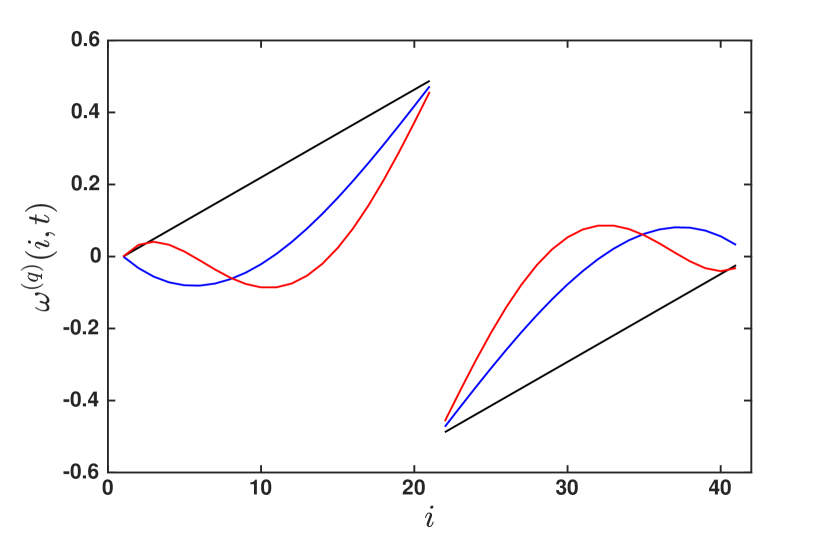
Figure 6: The weights of the residual $\omega^{(q)}(i,t)$ for Eq. (75) for detrending order $q=0$ and $1$ (black line), $q=2$ and $3$ (blue line) and $q=4$ and $5$ (red line). The segment length is $s=41$ and the time point is $t=(s+1)/2=21$. Note that for $t=(s+1)/2$ the weights are identical for $q=0$ and $1$ , $2$ and $3$ as well as $4$ and $5$ but not for other $t$, see figure 7.

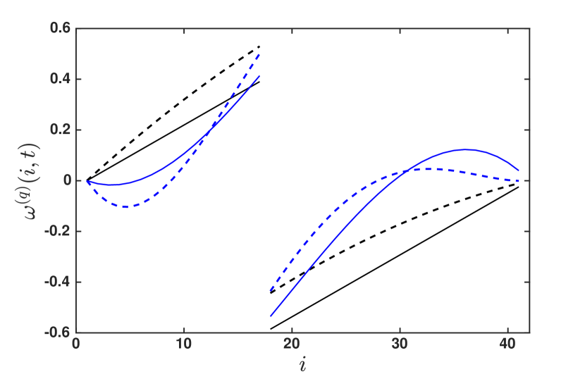
Figure 7: The weights of the residual $\omega^{(q)}(i,t)$ for Eq. (75) for detrending order $q=0$ (solid black line), $1$ (dashed black line), $2$ (solid blue line) and $3$ (dashed blue line). The segment length is $s=41$ and the time point is $t=17$.

VI.3 Scaling of the fluctuation function

Before we continue with our investigation we summarize published results about analytical derivations of the scaling behaviour of the fluctuation function $F^{2}(s)\sim s^{2\alpha}$, i.e. the derivation of $\alpha$ for specific processes. For DFA using the original definition of the fluctuation function: WN hoell AR($1$) hoell , FGN taqqu2 ; bardet ; movahed2 ; crato , BM hoell and FBM movahed ; heneghan ; kiyono . For DFA using the increment representation: WN, AR($1$) and ARFIMA($0$,$d$,$0$) hoell2 . For DMA using the original definition of the fluctuation function: FGN arianos ; arianos2 ; carbone . Although we are not aware of any analytical investigation of additive trends and FBM using the increment representation, we here restrict ourselves to stationary processes. We present simultaneously the investigation for DFA and DMA.

First we order the fluctuation function in the increment representation $F^{2}(s)=\sum_{i,j=1}^{s}\text{Cov}(i,j)L(i,j,s)$ according to the time lag $\tau$, namely

$$\begin{split}F^{2}(s)&=\sum_{i=1}^{s}\text{Cov}(i,i)L(i,i,s)\\ &+2\sum_{\tau=1}^{s-1}\sum_{i=1}^{s-\tau}\text{Cov}(i,i+\tau)L(i,i+\tau,s)\end{split}$$ (80)

For stationary processes the autocovariance function $\text{Cov}(i,j)$ only depends on the time lag $\tau$ and not the time point $i$. Therefore we can write this equation as

$$F^{2}(s)=\langle x^{2}(i)\rangle\left(\mathcal{L}(0,s)+2\sum_{\tau=1}^{s-1}C(\tau)\mathcal{L}(\tau,s)\right)$$ (81)

with the weights for the stationary fluctuation function

$$\mathcal{L}(\tau,s)=\sum_{i=1}^{s-\tau}L(i,i+\tau,s),$$ (82)

see figure 8 and 9. In appendix C we provide a detailed investigation of the weights of DMA $\mathcal{L}_{\text{DMA}q}(\tau,s)$. We also provide a Mathematica code for the calculation of $\mathcal{L}(\tau,s)$ for DMA in appendix E.E.7 and DFA in appendix E.E.8 for any order of detrending. As example we present the weight for DFA and zero order of detrending

$$\mathcal{L}_{\text{DFA}0}(\tau,s)=\frac{-\tau^{3}+3s\tau^{2}+(1-3s^{2})\tau+s^{3}-s}{6s^{2}}.$$ (83)

We also provide a Mathematica code for the calculation of $F^{2}(s)$ of Eq. (81) for DMA in appendix E.E.9 and DFA in appendix E.E.10 for any order of detrending and adjustable autocorrelation function. We tested the code for white noise, AR($1$) and ARFIMA($0$,$d$,$0$) processes. The asymptotic scaling behaviour of these explicit solutions is $2\alpha$ and we can therefore identify the fluctuation parameter for large $s$.

We also can understand the asymptotic behaviour of the fluctuation function directly from Eq. (81), see hoell2 for the DFA fluctuation function. The same argumentation as in hoell2 holds also for the DMA fluctuation function as it is presented for both methods in the following for uncorrelated and long-range correlated processes. For uncorrelated processes as white noise the autocorrelation function is nonzero only for $\tau=0$ and therefore the scaling is determined by the first part $\mathcal{L}(0,s)$ of Eq. (81) which scales linearly

$$F^{2}(s)\sim\mathcal{L}(0,s)\sim s.$$ (84)

Hence the fluctuation function scales with the fluctuation parameter $\alpha=1/2$ as it is claimed by the first principle (L1). In contrast for long-range correlated processes with autocorrelation function $C(\tau)\sim\tau^{-\gamma}$ with correlation parameter $0<\gamma<1$ the sum over $\tau$ in Eq. (81) dominates the asymptotic scaling behaviour

$$F^{2}(s)\sim\sum_{\tau=1}^{s-1}C(\tau)\mathcal{L}(\tau,s)=\sum_{\tau=1}^{s-1}s^{-\gamma}\mathcal{L}(\tau,s)\sim s^{2-\gamma}.$$ (85)

Hence the fluctuation function scales with fluctuation parameter $\alpha=1-\gamma/2$ which is also in accordance with the first principle (L1).

Figure 8: The weights of the stationary DFA fluctuation function $\mathcal{L}_{\text{DFA}q}$ of Eq. (82) for detrending order $q=0$ (black line), $1$ (blue line) and $2$ (red line). Here it is $s=41$.

Figure 9: The weights of the stationary DFA fluctuation function $\mathcal{L}_{\text{DFA}q}$ of Eq. (82) for detrending order $q=0$ and $1$ (black line), $2$ and $3$ (blue line) as well as $4$ and $5$ (red line). Here it is $s=41$.

VI.3.1 Crossover behaviour of autoregressive processes

Stationary processes with an autoregressive part like ARMA and ARFIMA processes show a crossover behaviour of the fluctuation function where only asymptotically the scaling exponent of $2\alpha$ is reached. For DFA applied on an AR($1$) process this has been investigated in hoell ; maraun . In hoell it has been shown that the second part $\sum_{\tau=1}^{s-1}C(\tau)\mathcal{L}(\tau,s)$ dominates the scaling of $F^{2}(s)$ for small enough $s$ due to the nonzero and exponential decaying autocorrelation function. In this small $s$ regime the scaling exponent is larger than $2\alpha$. Only for large enough $s$ the scaling of the AR($1$) fluctuation function goes over to that of the white noise case because then $\sum_{\tau=1}^{s-1}C(\tau)\mathcal{L}(\tau,s)$ becomes sufficiently small in comparison to $\mathcal{L}(0,s)$. We also observe numerically a crossover behaviour for an ARFIMA($1$,$d$,$0$) process which serves as example of a stationary long-range correlated process with an autoregressive part. But here we cannot explain in detail the crossover behaviour since we are not aware of a full analytical solution of the fluctuation function because of the quite complicated form of the autocorrelation function.

Such crossover behaviour requires a relatively large amount of data in order to observe the correct scaling. If there is not enough data then it is difficult to distinguish between short-range and long-range correlations using detrending methods for fluctuations meyer ; hoell .

VI.4 Unbiasedness of the estimator

In order to check the biasedness of the estimator of the fluctuation function we take the mean of the estimator $\langle\widehat{F^{2}}(s)\rangle$ and compare the difference to the fluctuation function $F^{2}(s)$. $\langle\widehat{F^{2}}(s)\rangle$ depends on the autocovariance function of the time series $\langle x(i+d_{\nu})x(j+d_{\nu})\rangle$. If there is no difference then the estimator is unbiased and can detect the scaling of the fluctuation function.

VI.4.1 Stationarity

For stationary processes the autocovariance function of the time series $\langle x(i+d_{\nu})x(j+d_{\nu})\rangle$ is independent of the shift factor $d_{v}$. This means it is the autocovariance function of the stochastic process $\langle x(i+d_{\nu})x(j+d_{\nu})\rangle=\text{Cov}(i,j)$ and therefore the estimator is unbiased $\langle\widehat{F^{2}}(s)\rangle=F^{2}(s)$ and the estimator obtains the scaling as explained in section VI.3.

VI.4.2 Intrinsic nonstationarity

As example of an intrinsic nonstationary process we investigate here FBM with the autocovariance function

$$\text{Cov}(i,j)=\frac{1}{2}\left(i^{2H}+j^{2H}-|i-j|^{2H}\right).$$ (86)

This problem has already been investigated for DFA in hoell3 . But there only the first and second segment has been compared and not all. Here we treat all segments and also the method of DMA. The autocovariance difference between segments $D_{\nu}(i,j)=\langle x(i+d_{\nu})x(j+d_{\nu})\rangle-\text{Cov}(i,j)$ with $\langle x(i+d_{\nu})x(j+d_{\nu})\rangle=\text{Cov}(i+d_{\nu},j+d_{\nu})$ is

$$D_{\nu}(i,j)=\frac{1}{2}\left((i+d_{\nu})^{2H}+(j+d_{\nu})^{2H}-i^{2H}-j^{2H}\right).$$ (87)

We show in appendix D that this can be written as infinite series

$$D_{\nu}(i,j)=\sum_{p=0}^{\infty}\lambda_{p}(i^{p}+j^{p})$$ (88)

using a Taylor expansion. The prefactors $\lambda_{p}$ depend on $H$, $d_{\nu}$ and an arbitrary point where the Taylor series is evaluated at, see appendix D. In hoell3 another series expansion using binomial series for $D_{2}(i,j)$ with DFA shift factor $d_{2}=s$ was proposed. But this series expansion does not converge always with the DMA shift factor whereas Eq. (88) does.

With Eq. (88) we can now check the biasedness of the estimator, namely by taking the mean of Eq. (63) which gives $\langle\widehat{F^{2}}(s)\rangle=1/K\sum_{\nu=1}^{K}\langle f_{\nu}^{2}(s)\rangle$. The mean of the estimator of the generalised squared path displacement is

$$\langle f_{\nu}^{2}(s)\rangle=\sum_{i,j=1}^{s}\text{Cov}(i,j)L(i,j,s)+\sum_{i,j=1}^{s}D_{\nu}(i,j)L(i,j,s)$$ (89)

where we used the splitting of $\langle x(i+d_{\nu})x(j+d_{\nu})\rangle$. With the Mathematica code for the calculation of $\langle f_{\nu}^{2}(s)\rangle$ for DMA in appendix E.E.4 and for DFA in appendix E.E.5 we verified that

$$\sum_{i,j=1}^{s}(i^{p}+j^{p})L(i,j,s)=0$$ (90)

for $p\in[1,50]$ and also particular higher values of $p$. Hence it is reasonable to assume that this equation holds for all $p$. We found that Eq. (90) is only zero for the detrending order $q\geq 1$ for DFA and $q\geq 0$ for DMA. In those cases the estimator is unbiased $\langle\widehat{F^{2}}(s)\rangle=F^{2}(s)$ because the bias is zero $B(s)=0$ due to Eq. (90). Finally, no matter if $\langle f_{\nu}^{2}(s)\rangle$ is zero or not, we also provide a Mathematica code for the calcuation of $\langle\widehat{F^{2}}(s)\rangle=1/K\sum_{\nu=1}^{K}\langle f_{\nu}^{2}(s)\rangle$ in appendix E.E.6. But due to the complicated form of the right hand side of Eq. (89) the code will not always be successfully yielding a result.

VI.4.3 External nonstationarity

As an example of an external nonstationarity we investigate additive trends $\{m(t)\}_{t=1}^{N}$ of order $p$, i.e. $m(t)\sim t^{p}$. The following is similar to the investigation of FBM from the previous section. The autocovariance difference is

$$D_{\nu}(i,j)=m(i+d_{\nu})m(j+d_{\nu}).$$ (91)

With the Mathematica code for the calculation of $\langle f_{\nu}^{2}(s)\rangle$ for DMA in appendix E.E.4 and for DFA in appendix E.E.5 we checked if the generalised squared path displacement applied on the autocovariance differences is zero,

$$\sum_{i,j=1}^{s}m(i+d_{\nu})m(j+d_{\nu})L(i,j,s)=0,$$ (92)

or not. We checked orders of the trend $p\in[1,6]$. For DFA this equation is zero if the order of detrending is $q\geq p+1$. For DMA it is $q\geq p+1$ for odd $p$ and $q\geq p$ for even $p$, this has also been found in carbone . For those cases the estimator of the fluctuation function is unbiased $\langle\widehat{F^{2}}(s)\rangle=F^{2}(s)$ because the bias is zero $B(s)=0$ due to Eq. (92).

VI.4.4 Unified picture of detrending

For both methods DFA and DMA the detrending procedure works similarly for two different types of nonstationarity, namely FBM and additive trends. After segmentation of the time axis the autocovariance function of the time series $\langle x(i+d_{\nu})x(j+d_{\nu})\rangle$ is different in every segment due to the shift factor $d_{\nu}$. This difference is described by the autocovariance differences $D_{\nu}(i,j)$. And since the estimation of the fluctuation function depends on the product $x(i+d_{\nu})x(j+d_{\nu})$ it is necessary that a successful detrending procedure gets rid of the influence of $D_{\nu}(i,j)$. If that is the case then the estimator of the fluctuation function is unbiased and therefore fulfills the second principle (L2). And exactly then the estimator of the fluctuation function can detect the fluctuation parameter $\alpha$ as described in the first principle (L1) even for those two different types of nonstationarity.

VII Summary

We provided three main points in this article of which all of them are similarly relevant and also linked with each other. First we motivated the introduction of detrending methods started from basic statistical methods. We introduced the fluctuation function as modified path MSD written in the increment representation, i.e. the connection between the fluctuation function and autocovariance function. Originally DFA and DMA provide an estimator of the fluctuation function in a form for which several points are unclear: the connection to the autocovariance function, the scaling behaviour and the ability of treating FBM. Especially the last two points are disadvantageous. The reason for this original description of the estimator of the fluctuation function is that these methods evolved from prior methods. But in the increment representation those two points can be handled which led us to the second main point: the description of detrending methods via two basic principles. The first principle ensures that the fluctuation function scales asymptotically similar to the path MSD. The second principles ensures that the estimator of the fluctuation function is unbiased. This is the centerpiece of the detrending procedure and is carried by our construction of the fluctuation function using a modificiation of the path MSD. Without this modification, namely the weighting of the path MSD in the increment representation, the estimator of the path MSD fails for nonstationary time series. And third we showed in detail that DFA and DMA are indeed examples of detrending methods. We explicitly verified the fulfillment of the two basic principles for both methods. in summary, this article provides a basic overview of detrending methods which answered fundamental questions. Furthermore we believe that this work can serve as basis for finding advanced detrending methods depending on specific problems in time series analysis, such as dealing with periodic deterministic components in $x(t)$.

Appendix A Residual as weighted sum

Here we express the residual $y(t+d_{\nu})-p_{\nu}^{(q)}(t+d_{\nu})$ of Eq. (74) in dependence of the time series. First we rewrite the profile and then the fit. The profile is per definition

$$\begin{split}y(t+d_{\nu})&=\sum_{i=1}^{t+d_{\nu}}x(i)=\sum_{i=1}^{s+d_{\nu}}x(i)\Theta(t+d_{\nu}-i)\\ &=y(d_{\nu})+\sum_{i=1+d_{\nu}}^{s+d_{\nu}}x(i)\Theta(t+d_{\nu}-i)\\ &=y(d_{\nu})+\sum_{i=1}^{s}x(i+d_{\nu})\Theta(t-i).\end{split}$$ (93)

The polynomial fit in segment $\nu$ of order $q$ can be written as

$$p_{\nu}^{(q)}(t+d_{\nu})=y(d_{\nu})+\sum_{i=1}^{s}x(i+d_{\nu})P_{\nu}^{(q)}(i,t)$$ (94)

with the weights of the fit

$$P_{\nu}^{(q)}(i,t)=\sum_{m=0}^{q}(t+d_{\nu})^{m}\sum_{n=0}^{q}(\mathbb{S}_{\nu}^{-1})_{m+1,n+1}\sum_{k=i+d_{\nu}}^{s+d_{\nu}}k^{n},$$ (95)

see hoell3 . The inverse matrix elements can be calculated as $(\mathbb{S}_{\nu}^{-1})_{m+1,n+1}=(\text{adj}\mathbb{S}_{\nu})_{m+1,n+1}/\text{det}\mathbb{S_{\nu}}$ where $\text{adj}\mathbb{S}_{\nu}$ is the adjugate matrix of the $(q+1)\times(q+1)$ matrix $\mathbb{S}_{\nu}$. The matrix $\mathbb{S}_{\nu}$ has the elements $S_{mn,\nu}=\sum_{i=1+d_{\nu}}^{s+d_{\nu}}i^{m+n-2}.$ Note that we wrote $\mathbb{S}=\mathbb{S}_{1}$ in section VI.2. With the Mathematica code in appendix E.E.2 we tested several orders of detrending $q$ and always found that $P_{\nu}^{(q)}(i,t)$ is independent of the segment $\nu$. This was tested for $d_{\nu}=(\nu-1)s$ and $\nu-1$. Hence we assume this independence of the segment is true for all $q$. Therefore the residual is

$$y(t+d_{\nu})-p_{\nu}^{(q)}(t+d_{\nu})=\sum_{i=1}^{s}x(i+d_{\nu})\omega^{(q)}(i,t)$$ (96)

with the weights of the residual

$$\omega^{(q)}(i,t)=\Theta(t-i)-P_{1}^{(q)}(i,t).$$ (97)

Appendix B $\boldsymbol{f_{\nu}^{2}(s)}$ in the increment representation

The estimators of the generalised squared path displacement $f_{\nu}^{2}(s)$ of DMA of Eq. (72) and DFA of Eq. (73) are written in their original description. Here we write them in the increment representation $f_{\nu}^{2}(s)=\sum_{i,j=1}^{s}x(i+d_{\nu})x(j+d_{\nu})L(i,j,s)$, see Eq. (62). We find the specific forms of the weights $L(i,j,s)$ for DMA and DFA.

B.1 $\boldsymbol{f_{\nu}^{2}(s)}$ of DMA in the increment representation

In the following we use for the middle point of the first segment the notation $\sigma=(s+1)/2$. For DMA the estimator of the generalised squared path displacement is

$$\begin{split}f^{2}_{\nu,\text{DMA$q$}}(s)=\left(y(\sigma+d_{\nu,\text{DMA}})-p_{\nu}^{(q)}(\sigma+d_{\nu,\text{DMA}})\right)^{2},\end{split}$$ (98)

see Eq. (72). Using the residual as weighted sum given in Eq. (96) we can write this as

$$\begin{split}&f_{\nu,\text{DMA$q$}}^{2}(s)\\ &=\left(\sum_{i=1}^{s}x(i+d_{\nu,\text{DMA}})\omega^{(q)}(i,\sigma)\right)^{2},\\ &=\sum_{i,j=1}^{s}x(i+d_{\nu,\text{DMA}})x(j+d_{\nu,\text{DMA}})\omega^{(q)}(i,\sigma)\omega^{(q)}(j,\sigma).\end{split}$$ (99)

Hence the weights of DMA are

$$L_{\text{DMA}q}(i,j,s)=\omega^{(q)}(i,\sigma)\omega^{(q)}(j,\sigma)$$ (100)

which has breaks due to the Heaviside function. In detail $f_{\nu,\text{DMA$q$}}^{2}(s)$ is given by

$$\begin{split}&f_{\nu,\text{DMA}q}^{2}(s)\\ &=\sum_{i=1}^{\sigma}\Big{[}x^{2}(i+d_{\nu,\text{DMA}})\left(1-P_{1}^{(q)}(i,\sigma)\right)^{2}\Big{]}\\ &+\sum_{i=\sigma+1}^{s}\Big{[}x^{2}(i+d_{\nu,\text{DMA}})\left(P_{1}^{(q)}(i,\sigma)\right)^{2}\Big{]}\\ &+2\sum_{i=1}^{\sigma}\sum_{j=i+1}^{\sigma}\Big{[}x(i+d_{\nu,\text{DMA}})x(j+d_{\nu,\text{DMA}})\\ &\hskip 42.67912pt\times\left(1-P_{1}^{(q)}(i,\sigma)\right)\left(1-P_{1}^{(q)}(j,\sigma)\right)\Big{]}\\ &+2\sum_{i=1}^{\sigma}\sum_{j=\sigma+1}^{s}\Big{[}x(i+d_{\nu,\text{DMA}})x(j+d_{\nu,\text{DMA}})\\ &\hskip 42.67912pt\times\left(1-P_{1}^{(q)}(i,\sigma)\right)\left(-P_{1}^{(q)}(j,\sigma)\right)\Big{]}\\ &+2\sum_{i=\sigma+1}^{s-1}\sum_{j=i+1}^{s}\Big{[}x(i+d_{\nu,\text{DMA}})x(j+d_{\nu,\text{DMA}})\\ &\hskip 42.67912pt\times P_{1}^{(q)}(i,\sigma)P_{1}{(q)}(j,\sigma)\Big{]}.\end{split}$$ (101)

B.2 $\boldsymbol{f_{\nu}^{2}(s)}$ of DFA in the increment representation

For DFA the estimator of the generalised squared path displacement is

$$\begin{split}&f^{2}_{\nu,\text{DFA$q$}}(s)\\ &=\frac{1}{s}\sum_{t=1}^{s}\Big{(}y(t+d_{\nu,\text{DFA}})-p_{\nu}^{(q)}(t+d_{\nu,\text{DFA}})\Big{)}^{2},\end{split}$$ (102)

see Eq. (73). Using the residual as weighted sum given in Eq. (96) we can write this as

$$\begin{split}&f_{\nu,\text{DFA}q}^{2}(s)\\ &=\frac{1}{s}\sum_{t=1}^{s}\left(\sum_{i=1}^{s}x(i+d_{\nu,\text{DFA}})\omega^{(q)}(i,t)\right)^{2},\\ &=\sum_{i,j=1}^{s}x(i+d_{\nu,\text{DFA}})x(j+d_{\nu,\text{DFA}})\\ &\hskip 42.67912pt\times\frac{1}{s}\sum_{t=1}^{s}\omega^{(q)}(i,t)\omega^{(q)}(j,t).\end{split}$$ (103)

Hence the weights of the DFA fluctuation function are

$$L_{\text{DFA}q}(i,j,s)=\frac{1}{s}\sum_{t=1}^{s}\omega^{(q)}(i,t)\omega^{(q)}(j,t)$$ (104)

which has no breaks in contrast to the weights of DMA. In detail for $j>i$ it can be written as

$$\begin{split}&L_{\text{DFA}q}(i,j,s)\\ &=\frac{1}{s}\Bigg{(}\sum_{t=j}^{s}1-\sum_{t=i}^{s}P-1^{(q)}(j,t)\\ &-\sum_{t=j}^{s}P_{1}^{(q)}(i,t)+\sum_{t=1}^{s}P_{1}^{(q)}(i,t)P_{1}^{(q)}(j,t)\Bigg{)}.\end{split}$$ (105)

The restriction $j>i$ is no problem because the double sum $\sum_{i,j=1}^{s}$ can ordered such that only terms with $j>i$ occur, see Eq. (128).

Appendix C Stationary DMA fluctuation function

The fluctuation function of DMA for stationary processes is given by

$$\begin{split}F_{\text{DMA}q}^{2}(s)&=\langle x^{2}(i)\rangle\Big{(}\mathcal{L}_{\text{DMA}q}(0,s)\\ &+2\sum_{\tau=1}^{s-1}C(\tau)\mathcal{L}_{\text{DMA}q}(\tau,s)\Big{)},\end{split}$$ (106)

see Eq. (81) which can be written more detailed as follows. The weights $\mathcal{L}_{\text{DMA}q}(\tau,s)$ have different expressions depending on the time lag $\tau$. This can be derived by using $L_{\text{DMA}q}(i,j,s)$ of Eq. (100) in $\mathcal{L}_{\text{DMA}q}(\tau,s)=\sum_{i=1}^{s-\tau}L_{\text{DMA}q}(i,i+\tau,s)$ of Eq. (82). Again $\sigma=(s+1)/2$. Hence we find the following. For $1\leq\tau\leq\sigma-2$ it is

$$\begin{split}&\mathcal{L}_{\text{DMA}q}(\tau,s)\\ &=\sum_{i=1}^{\sigma-\tau}\left(1-P_{1}^{(q)}(i,\sigma)\right)\left(1-P_{1}^{(q)}(i+\tau,\sigma)\right)\\ &+\sum_{i=\sigma-\tau+1}^{\sigma}\left(1-P_{1}^{(q)}(i,\sigma)\right)\left(-P_{1}^{(q)}(i+\tau,\sigma)\right)\\ &+\sum_{i=\sigma+1}^{s-\tau}P_{1}^{(q)}(i,\sigma)P_{1}^{(q)}(i+\tau,\sigma).\end{split}$$ (107)

For $\tau=\sigma-1$ it is

$$\begin{split}&\mathcal{L}_{\text{DMA}q}(\tau,s)\\ &=\sum_{i=1}^{\sigma-\tau}\left(1-P_{1}^{(q)}(i,\sigma)\right)\left(1-P_{1}^{(q)}(i+\tau,\sigma)\right)\\ &+\sum_{i=\sigma-\tau+1}^{s-\tau}\left(1-P_{1}^{(q)}(i,\sigma)\right)\left(-P_{1}^{(q)}(i+\tau,\sigma)\right).\end{split}$$ (108)

For $\sigma\leq\tau\leq s-1$ it is

$$\begin{split}&\mathcal{L}_{\text{DMA}q}(\tau,s)\\ &=\sum_{i=1}^{s-\tau}\left(1-P_{1}^{(q)}(i,\sigma)\right)\left(-P_{1}^{(q)}(i+\tau,\sigma)\right).\end{split}$$ (109)

Let us write the weights of Eq. (LABEL:w1), (LABEL:w2) and (LABEL:w3) as $\mathcal{L}_{\text{DMA}q}^{(1)}(\tau,s)$, $\mathcal{L}_{\text{DMA}q}^{(2)}(\tau,s)$ and $\mathcal{L}_{\text{DMA}q}^{(3)}(\tau,s)$. Then the statioary fluctuation function of Eq. (106) is given in detail by

$$\begin{split}&F_{\text{DMA}q}^{2}(s)\\ &=\langle x^{2}(i)\rangle\Bigg{(}\mathcal{L}_{\text{DMA}q}^{(1)}(0,s)+2\sum_{\tau=1}^{\sigma-2}C(\tau)\mathcal{L}_{\text{DMA}q}^{(1)}(\tau,s)\\ &+2\sum_{\tau=\sigma-1}^{\sigma-1}C(\tau)\mathcal{L}_{\text{DMA}q}^{(2)}(\tau,s)+2\sum_{\tau=\sigma}^{s-1}C(\tau)\mathcal{L}_{\text{DMA}q}^{(3)}(\tau,s)\Bigg{)}.\end{split}$$ (110)

Appendix D Autocovoariance difference of FBM

The autocovariance difference of FBM is

$$D_{\nu}(i,j)=\frac{1}{2}\left((i+d_{\nu})^{2H}+(j+d_{\nu})^{2H}-i^{2H}-j^{2H}\right),$$ (111)

see Eq. (87). We can write $(i+d_{\nu})^{2H}-i^{2H}$ as infinite sum

$$(i+d_{\nu})^{2H}-i^{2H}=\sum_{m=0}^{\infty}i^{m}(v_{m}(h,d_{\nu},r)-v_{m}(h,0,r))$$ (112)

using Taylor’s series, see appendix D.D.1 for the definition of $v_{m}$. The same holds for the $j$-dependent term of $D_{\nu}(i,j)$. Hence we can write the autocovariance difference as

$$D_{\nu}(i,j)=\sum_{m=0}^{\infty}(i^{m}+j^{m})(v_{m}(h,d_{\nu},r)-v_{m}(h,0,r)).$$ (113)

Note that $r$ can be chosen arbitrarily. In section VI.4.2 we use the definition $\lambda_{m}=v_{m}(h,d_{\nu},r)-v_{m}(h,0,r)$.

D.1 Taylor series

For the function

$$f(i)=(i+d)^{h}$$ (114)

with constants $d\geq 0$ and $h>0$ the Taylor series at point $r$ is

$$f(i)=\sum_{n=0}^{\infty}\frac{f^{(n)}(i_{0})}{n!}(i-r)^{n}.$$ (115)

With the derivative

$$f^{(n)}(i)=\begin{pmatrix}h\\ n\end{pmatrix}n!(i+d)^{h-n}.$$ (116)

the function is

$$f(i)=\sum_{n=0}^{\infty}\begin{pmatrix}h\\ n\end{pmatrix}(r+d)^{h-n}(i-r)^{n}.$$ (117)

Using binomial theorem for the term

$$(i-r)^{n}=\sum_{m=0}^{n}\begin{pmatrix}n\\ m\end{pmatrix}(-r)^{n-m}i^{n}.$$ (118)

the function is

$$f(i)=\sum_{n=0}^{\infty}\sum_{m=0}^{n}\begin{pmatrix}h\\ n\end{pmatrix}\begin{pmatrix}n\\ m\end{pmatrix}(r+d)^{h-n}(-r)^{n-m}i^{m}.$$ (119)

This can be ordered with respect to $i$, namely

$$f(i)=\sum_{m=0}^{\infty}i^{m}v_{m}(h,d,r)$$ (120)

with

$$v_{m}(h,d,r)=\sum_{n=m}^{\infty}\begin{pmatrix}h\\ n\end{pmatrix}\begin{pmatrix}n\\ m\end{pmatrix}(r+d)^{h-n}(-r)^{n-m}.$$ (121)

If $d=0$ we pick a nonzero point $r\neq 0$.

Appendix E Mathematica codes

Here we provide Mathematica codes for important quantitites of this article. They can easily be used by simply copying the source code into Mathematica and execute them. We indicate the begin of a line in the code with (**) for the sake of clarity. Furthermore we explain how the codes can be modified to get different outputs.

E.1 Weights of the first fit

Here we provide the Mathematica code for the weights of the fit with $\nu=1$, namely

$$P_{1}^{(q)}(i,t)=\sum_{m=0}^{q}t^{m}\sum_{n=0}^{q}\left(\mathbb{S}_{1}^{-1}\right)_{m+1,n+1}\sum_{k=i}^{s}k^{n},$$ (122)

see Eq. (95). This is calculated by the following Mathematica code:

(**)q=0;
(**)S[i_]:=Sum[k^i,{k,1,s}];
(**)matrixS:=Table[S[m+n-2],{m,q+1},{n,q+1}];
(**)Simplify[Sum[t^m*Sum[Inverse[matrixS][[
    m+1,n+1]]*Sum[k^n,{k,i,s}],{n,0,q}],{
    m,0,q}]]
    

The output of this code gives $P_{1}^{(0)}(i,t)$ with order of detrending $q=0$. The order of detrending $q$ in the first line "q=0;" can be changed to any order, e.g. to "q=1;" for first order of detrending. Note that $P_{1}^{(q)}(i,t)$ is the same for DFA and DMA.

E.2 Weights of the fits

Here we provide the Mathematica code for the weights of the fit for DFA and DMA

$$P_{\nu}^{(q)}(i,t)=\sum_{m=0}^{q}(t+d_{\nu})^{m}\sum_{n=0}^{q}(\mathbb{S}_{\nu}^{-1})_{m+1,n+1}\sum_{k=i+d_{\nu}}^{s+d_{\nu}}k^{n},$$ (123)

see Eq. (95). This is calculated by the following Mathematica code:

(**)q=0;
(**)d[v_]:=(v-1)*s;
(**)S[i_]:=Sum[k^i,{k,1+d[v],s+d[v]}];
(**)matrixS:=Table[S[m+n-2],{m,q+1},{n,q+1}];
(**)Simplify[Sum[(t+d[v])^m*Sum[Inverse[
    matrixS][[m+1,n+1]]*Sum[k^n,{k,i+d[v],s+
    d[v]}],{n,0,q}],{m,0,q}]]

The output of this code gives $P_{\nu,\text{DFA}}^{(0)}(i,t)$ with order of detrending $q=0$ and DFA shift factor $d_{\nu,\text{DFA}}=(\nu-1)s$. The order of detrending in first line "q=0;" can be changed to any order, e.g. to "q=1;" for first order of detrending. The DFA shift factor in the second line "d[v_]:=(v-1)*s;" can be changed to the DMA shift factor "d[v_]:=v-1;". Note that $P_{\nu}^{(q)}(i,t)$ is the same for DFA and DMA.

E.3 Weights of DFA fluctuation function

Here we provide the Mathematica code for the weights of the DFA fluctuation function with $j>i$, namely

$$\begin{split}&L_{\text{DFA}q}(i,j,s)\\ &=\frac{1}{s}\Bigg{(}\sum_{t=j}^{s}1-\sum_{t=i}^{s}P_{1}^{(q)}(j,t)\\ &-\sum_{t=j}^{s}P_{1}^{(q)}(i,t)+\sum_{t=1}^{s}P_{1}^{(q)}(i,t)P_{1}^{(q)}(j,t)\Bigg{)},\end{split}$$ (124)

see Eq. (LABEL:dfaweight65). This is calculated by the following Mathematica code:

(**)P[i_,t_]:=(1-i+s)/s;
(**)Simplify[1/s*(Sum[1,{t,j,s}]-Sum[P[j,t],
    {t,i,s}]-Sum[P[i,t],{t,j,s}]+Sum[P[i,t]*
    P[j,t],{t,1,s}])]

The output of this code gives $L_{\text{DFA}0}(i,j,s)$ using the output from appendix E.E.1 which is the weight of the fit $P_{1}^{(0)}(i,t)=(1-i+s)/s$. This output from appendix E.E.1 in the first line "(1-i+s)/s" can be changed to any output from the code of appendix E.E.1 by changing the definition of "q" in the code of appendix E.E.1 as explained there.

E.4 $\boldsymbol{\langle f_{\nu}^{2}(s)\rangle}$ of DMA

Here we provide the Mathematica code for the mean of the estimator of the generalised squared path displacement of DMA in the increment representation

$$\langle f^{2}_{\nu,\text{DMA}q}(s)\rangle=\sum_{i,j=1}^{s}G_{\nu}(i,j)L_{\text{DMA}q}(i,j,s),$$ (125)

see Eq. (LABEL:ret3). The function $G_{\nu}(i,j)$ can in principle be arbitrary. Here in the article it is $G_{\nu}(i,j)=\langle x(i+d_{\nu,\text{DMA}})x(j+d_{\nu,\text{DMA}})\rangle$, $\text{Cov}(i,j)$ and $D_{\nu}(i,j)$. But due to the possible complicated form of $G_{\nu}(i,j)$ the code will not always be succesfully calculating a result. With the help of Eq. (LABEL:fdmadetail) it is now in detail

$$\begin{split}&\langle f^{2}_{\nu,\text{DMA}q}(s)\rangle\\ &=\sum_{i=1}^{\sigma}\Big{[}G_{\nu}(i,i)\left(1-P_{1}^{(q)}(i,\sigma)\right)^{2}\Big{]}\\ &+\sum_{i=\sigma+1}^{s}\Big{[}G_{\nu}(i,i)\left(P_{1}^{(q)}(i,\sigma)\right)^{2}\Big{]}\\ &+2\sum_{i=1}^{\sigma}\sum_{j=i+1}^{\sigma}\Big{[}G_{\nu}(i,j)\\ &\hskip 42.67912pt\times\left(1-P_{1}^{(q)}(i,\sigma)\right)\left(1-P_{1}^{(q)}(j,\sigma)\right)\Big{]}\\ &+2\sum_{i=1}^{\sigma}\sum_{j=\sigma+1}^{s}\Big{[}G_{\nu}(i,j)\\ &\hskip 42.67912pt\times\left(1-P_{1}^{(q)}(i,\sigma)\right)\left(-P_{1}^{(q)}(j,\sigma)\right)\Big{]}\\ &+2\sum_{i=\sigma+1}^{s-1}\sum_{j=i+1}^{s}\Big{[}G_{\nu}(i,j)P_{1}^{(q)}(i,\sigma)P_{1}^{(q)}(j,\sigma)\Big{]}.\end{split}$$ (126)

This is calculated by the following Mathematica code:

(**)P[i_,t_]:=(1-i+s)/s;
(**)d[v_]=v-1;
(**)p=1;
(**)G[i_,j_,v_]:=(i+d[v])^p*(j+d[v])^p;
(**)sigma=(s+1)/2;
(**)Simplify[Sum[G[i,i,v]*(1-P[i,sigma])^2,
    {i,1,sigma}]+Sum[G[i,i,v]*P[i,sigma]^2,
    {i,sigma+1,s}]+2*Sum[Sum[G[i,j,v]*(1-
    P[i,sigma])*(1-P[j,sigma]),{j,i+1,
    sigma}],{i,1,sigma}]+2*Sum[Sum[G[i,j,
    v]*(1-P[i,sigma])*(-P[j,sigma]),{j,
    sigma+1,s}],{i,1,sigma}]
    +2*Sum[Sum[G[i,j,v]*P[i,sigma]*P[j,
    sigma],{j,i+1,s}],{i,sigma+1,s-1}]]

The output of this code gives $\langle f^{2}_{\nu,\text{DMA}0}(s)\rangle$ using the output from appendix E.E.1 which is the weight of the fit $P_{1}^{(0)}(i,t)=(1-i+s)/s$ and the autocovariance difference of an additive trend $G_{ij}^{(\nu)}=(i+d_{\nu,\text{DMA}})^{p}(i+d_{\nu,\text{DMA}})^{p}$ of a trend with order $p=1$. The output from appendix E.E.1 in the first line "(1-i+s)/s" can be changed to any output from the code of appendix E.E.1 by changing the definition of "q" in the code of appendix E.E.1 as explained there. The autocovariance difference of the trend in the fourth line "(i+d[v])^p*(j+d[v])^p" can be changed to any $G_{\nu}(i,j)$, e.g. the autocovariance difference of FBM "i^p+j^p" where we left out the prefactors. The order of $p$ in the third line "p=1" can be changed to any order, e.q. to "p=2" for second order.

E.5 $\boldsymbol{\langle f_{\nu}^{2}(s)\rangle}$ of DFA

Here we provide the Mathematica code for the mean of the estimator of the generalised squared path displacement of DMA in the increment representation

$$\langle f^{2}_{\nu,\text{DFA}q}(s)\rangle=\sum_{i,j=1}^{s}G_{\nu}(i,j)L_{\text{DFA}q}(i,j,s),$$ (127)

see Eq. (LABEL:ret2). The function $G_{\nu}(i,j)$ can in principle be arbitrary. Here in the article it is $G_{\nu}(i,j)=\langle x(i+d_{\nu,\text{DFA}})x(j+d_{\nu,\text{DFA}})\rangle$, $\text{Cov}(i,j)$ and $D_{\nu}(i,j)$. But due to the possible complicated form the code will not always be succesfully calculating a result. We can order Eq. (127) to

$$\begin{split}\langle f^{2}_{\nu,\text{DFA}q}(s)\rangle&=\sum_{i=1}^{s}G_{\nu}(i,i)L_{\text{DFA}q}(i,i,s)\\ &+2\sum_{i=1}^{s-1}\sum_{j=i+1}^{s}G_{\nu}(i,j)L_{\text{DFA}q}(i,j,s)\end{split}$$ (128)

This is calculated by the following Mathematica code:

(**)L[i_,j_,s_]:=((-1+i) (1-j+s))/s^2;
(**)d[v_]=(v-1)*s;
(**)p=1;
(**)G[i_,j_,v_]:=(i+d[v])^p*(j+d[v])^p;
(**)Simplify[Sum[G[i,i,v]*L[i,i,s],{i,1,s}]
    +2*Sum[Sum[G[i,j,v]*L[i,j,s],{j,i+1,s}],
    {i,1,s-1}]]

The output of this code gives $\langle f^{2}_{\nu,\text{DFA}0}(s)\rangle$ using the output from appendix E.E.3 which is the weight of the fluctuation function $L_{\text{DFA}0}(i,j,s)=(i-1)(s-j+1)/s^{2}$ and the autocovariance difference of an additive trend $G_{ij}^{(\nu)}=(i+d_{\nu,\text{DMA}})^{p}(i+d_{\nu,\text{DMA}})^{p}$ of a trend with order $p=1$. The output from appendix E.E.3 in the first line "((-1+i) (1-j+s))/s^2" can be changed to any output from the code of appendix E.E.3 by changing the definition of "P[i_,t_]" in the code of appendix E.E.3 as explained there. The autocovariance difference of the trend in the fourth line "(i+d[v])^p*(j+d[v])^p" can be changed to any $G_{\nu}(i,j)$, e.g. the autocovariance difference of FBM "i^p+j^p" where we left out the prefactors. The order of $p$ in the third line "p=1" can be changed to any order, e.q. to "p=2" for second order.

E.6 $\boldsymbol{\langle\widehat{F^{2}}(s)\rangle}$ of DMA and DFA

Here we provide the Mathematica code for the mean of the estimator of the fluctuation function of DMA and DFA

$$\langle\widehat{F^{2}}(s)\rangle=\frac{1}{K}\sum_{\nu=1}^{K}\langle f^{2}_{\nu}(s)\rangle,$$ (129)

see Eq. (63). This is calculated by the following code:

(**)f[v_,s_]:=1/180(-1+s^2)(14+15s(-
    1+2v)+s^2(4-15v+15 v^2));
(**)k=n/s;
(**)Simplify[1/k*Sum[f[v,s],{v,1,k}]]

The output of this code gives $\langle\widehat{F^{2}}_{\text{DFA}0}(s)\rangle$ using $K=N/s$ and the output from appendix E.E.5 which is the mean of the estimator of the generalised squared path displacement of DFA $\langle f^{2}_{\nu,\text{DFA}0}(s)\rangle$. This output from appendix E.E.5 in the first line "1/180(-1+s^2..." can be changed to any output from the code of appendix E.E.5 by changing the definition of "L[i_,j_,s_]" in the code of appendix E.E.5 as explained there. Furthermore can the first line "1/180(-1+s^2..." be changed to the output from the code of appendix E.E.4 which is the mean of the estimator of the generalised squared path displacement of DMA $\langle f^{2}_{\nu,\text{DMA}0}(s)\rangle$. This output from appendix E.E.4 can be changed to any output from the code of appendix E.E.4 by changing the definition of "P[i_,t_]" in the code of appendix E.E.4 as explained there. For DMA the second line "k=n/s" has to be changed to "k=n-s+1".

E.7 Weights of stationary DMA fluctuation function

Here we provide the Mathematica code for the weights of the stationary fluctuation function of DMA $\mathcal{L}_{\text{DMA}q}^{(1)}(\tau,s)$, $\mathcal{L}_{\text{DMA}q}^{(2)}(\tau,s)$ and $\mathcal{L}_{\text{DMA}q}^{(3)}(\tau,s)$, see for their explicit forms Eq. (LABEL:w1), (LABEL:w2) and (LABEL:w3) in appendix C. These are calculated by the following code:

(**)P[i_,t_]:=(1-i+s)/s;
(**)sigma=(s+1)/2;
(**)Simplify[Sum[(1-P[i,sigma])*(1-P[i
    +tau,sigma]),{i,1,sigma-tau}]+Sum[
    (1-P[i,sigma])*(-P[i+tau,sigma]),
    {i,sigma-tau+1,sigma}]+Sum[P[i,
    sigma]*P[i+tau,sigma],{i,sigma+1,
    s-tau}]]
(**)Simplify[Sum[(1-P[i,sigma])*(1-P[i
    +tau,sigma]),{i,1,sigma-tau}]+Sum[
    (1-P[i,sigma])*(-P[i+tau,sigma]),
    {i,sigma-tau+1,s-tau}]]
(**)Simplify[Sum[(1-P[i,sigma])*(-P[i+
    tau,sigma]),{i,1,s-tau}]]

The output of this code gives $\mathcal{L}_{\text{DMA}0}^{(1)}(\tau,s)$, $\mathcal{L}_{\text{DMA}0}^{(2)}(\tau,s)$ and $\mathcal{L}_{\text{DMA}0}^{(3)}(\tau,s)$ using the output from appendix E.E.1 which is the weight of the fit $P_{1}^{(0)}(i,t)=(1-i+s)/s$. This output from appendix E.E.1 in the first line "(1-i+s)/s" can be changed to any output from the code of appendix E.E.1 by changing the definition of "q" in the code of appendix E.E.1 as explained there.

E.8 Weights of stationary DFA fluctuation function

Here we provide the Mathematica code for the weights of the stationary fluctuation function of DFA

$$\mathcal{L}_{\text{DFA}q}(\tau,s)=\sum_{i=1}^{s-\tau}L_{\text{DFA}q}(i,i+\tau,s),$$ (130)

see Eq. (82). This is calculated by the following code:

(**)L[i_,j_,s_]:=((-1+i) (1-j+s))/s^2;
(**)Simplify[Sum[L[i,i+tau,s],{i,1,s-tau}]]

The output of this code gives $\mathcal{L}_{\text{DFA}0}(\tau,s)$ using the output from appendix E.E.3 which is the weight of the fluctuation function $L_{\text{DFA}0}(i,j,s)=(i-1)(s-j+1)/s^{2}$. This output from appendix E.E.3 in the first line "((-1+i) (1-j+s))/s^2" can be changed to any output from the code of appendix E.E.3 by changing the definition of "P[i_,t_]" in the code of appendix E.E.3 as explained there.

E.9 Stationary DMA fluctuation function

Here we provide the Mathematica code for the stationary fluctuation function of DMA

$$\begin{split}&F_{\text{DMA}q}^{2}(s)\\ &=\langle x^{2}(i)\rangle\Bigg{(}\mathcal{L}_{\text{DMA}q}^{(1)}(0,s)+2\sum_{\tau=1}^{\sigma-2}C(\tau)\mathcal{L}_{\text{DMA}q}^{(1)}(\tau,s)\\ &+2\sum_{\tau=\sigma-1}^{\sigma-1}C(\tau)\mathcal{L}_{\text{DMA}q}^{(2)}(\tau,s)+2\sum_{\tau=\sigma}^{s-1}C(\tau)\mathcal{L}_{\text{DMA}q}^{(3)}(\tau,s)\Bigg{)}.\end{split}$$ (131)

see Eq. (LABEL:statflucdmafull). This is calculated by the following code:

(**)c[tau_]:=a^tau/(1-a^2);
(**)sigma=(s+1)/2;
(**)L1[tau_]:=(s^3-6 s^2 tau+2 tau (-1+
    tau^2)+s (-1+6 tau^2))/(12 s^2);
(**)L2[tau_]:=(s-s^3-4 tau+4 tau^3)/
    (24 s^2);
(**)L3[tau_]:=-(((1+s-tau) (-s+s^2+tau-
    2 s tau+tau^2))/(6 s^2));
(**)Simplify[c[0]*L1[0]+2*Sum[c[tau]*
    L1[tau],{tau,1,sigma-2}]+2*Sum[c[
    tau]*L2[tau],{tau,sigma-1,sigma-1}]
    +2*Sum[c[tau]*L3[tau],{tau,sigma,s-1}]]

The output of this code gives $F_{\text{DMA}0}^{2}(s)$ using the autocorrelation function of an AR($1$) process $\text{Cov}(\tau)=a^{\tau}/(1-a^{2})$ with parameter $a$ and the outputs of appendix E.E.7 which are the weights of the stationary fluctuation function stationary of DMA $\mathcal{L}_{\text{DMA}0}^{(1)}(\tau,s)$, $\mathcal{L}_{\text{DMA}0}^{(2)}(\tau,s)$ and $\mathcal{L}_{\text{DMA}0}^{(3)}(\tau,s)$. The autocovariance function in the first line "c[tau_]:=a^tau/(1-a^2);" can be changed to any autocovariance function, e.g. the autocovariance function of white noise with unit variance "c[tau_]:=KroneckerDelta[tau,0];" or ARFIMA($0$,$d$,$0$). The autocovariance function of an ARFIMA($0$,$d$,$0$) is $\text{Cov}(\tau)=\Gamma(\tau+d)\Gamma(\tau-2d)/(\Gamma(\tau+1-d)\Gamma(1-d)\Gamma(d))$. The outputs from appendix E.E.7 in the third line "(s^3-6s^2tau+...", fourth line "(s-s^3-..." and fifth line "(((1+s-tau)..." can be changed to any outputs from appendix E.E.7 by changing the definition of "P[i_,t_]" in the code from appendix E.E.7 as explained there.

E.10 Stationary DFA fluctuation function

Here we provide the Mathematica code of the stationary fluctuation function of DFA

$$\begin{split}F_{\text{DFA}q}^{2}(s)&=\langle x^{2}(i)\rangle\Big{(}\mathcal{L}_{\text{DFA}q}(0,s)\\ &+2\sum_{\tau=1}^{s-1}C(\tau)\mathcal{L}_{\text{DFA}q}(\tau,s)\Big{)},\end{split}$$ (132)

see Eq. (81). This is calculated by the following code:

(**)c[tau_]:=a^tau/(1-a^2);
(**)L[tau_]:=((1+s-tau)(-s+s^2+tau-
    2 s tau+tau^2))/(6 s^2);
(**)Simplify[c[0]*L[0]+2*Sum[c[
    tau]*L[tau],{tau,1,s-1}]]

The output of this code gives $F_{\text{DFA}0}^{2}(s)$ using the autocorrelation function of an AR($1$) process $\text{Cov}(\tau)=a^{\tau}/(1-a^{2})$ with parameter $a$ and the output of appendix E.E.8 which are the weights of the stationary fluctuation function of DFA $\mathcal{L}_{\text{DFA}0}(\tau,s$.) The autocovariance function in the first line "c[tau_]:=a^tau/(1-a^2);" can be changed to any autocovariance function, e.g. the autocovariance function of white noise with unit variance "c[tau_]:=KroneckerDelta[tau,0];" or ARFIMA($0$,$d$,$0$). The autocovariance function of an ARFIMA($0$,$d$,$0$) is $\text{Cov}(\tau)=\Gamma(\tau+d)\Gamma(\tau-2d)/(\Gamma(\tau+1-d)\Gamma(1-d)\Gamma(d))$. The output from appendix E.E.8 in the second line "((1+s-tau)..." can be changed to any output from appendix E.E.8 by changing the definition of "L[i_,j_,s]" in the code from appendix E.E.8 as explained there.

References

- (1) H.E. Hurst, T. Am. Soc. Civ. Eng. 116, 770 (1951).
- (2) T. Graves, R. Gramacy, N. Watkins and C. Franzke, Entropy 19, 437 (2017).
- (3) W. Palma, Long-Memory Time Series, Wiley, 2007
- (4) J. Beran, Statistics for Long-Memory Processes, Chapmann & Hall, 1994
- (5) V. Pipiras and M.S. Taqqu, Long-Range Dependence and Self-Similarity, Cambridge University Press, 2017
- (6) J.W. Kantelhardt, E. Koscielny-Bunde, H.H.A. Rego, S. Havlin and A. Bunde, Physica A 295, 441 (2001).
- (7) C.K. Peng, S.V. Buldyrev, S. Havlin, M. Simons, H.E. Stanley and A.L. Goldberger, Phys. Rev. E 49, 1685 (1994).
- (8) T. Penzel, J.W. Kantelhardt, L. Grote, J.H. Peter and A. Bunde, IEEE T. Bio-Med. Eng. 50, 1143 (2003).
- (9) J.C. Echeverria, M.S. Woolfson, J.A. Crowe, B.R. Hayes-Gill, G.D.H. Croaker and H. Vyas, Chaos 13, 467 (2003).
- (10) P. Castiglioni, G. Parati, A. Civijian, L. Quintin, and M. Di Rienzo, IEEE T. Bio-Med. Eng. 56, 675 (2009).
- (11) M. Baumert, M. Javorka, A. Seeck, R. Faber, P. Sanders, and A. Voss, Comput. Biol. Med. 42, 347 (2012).
- (12) P. Talkner and R.O. Weber, Phys. Rev. E 62, 150 (2000).
- (13) A. Kiraly and I.M. Janosi, Meteorol. Atmos. Phys. 88, 119 (2005).
- (14) M.L. Kurnaz, Fractals 12, 365 (2004).
- (15) E. Koscielny-Bunde, A. Bunde, S. Havlin, H.E. Roman, Y. Goldreich and H.J. Schellnhuber, Phys. Rev. Lett. 81, 729 (1998).
- (16) P. Meyer, M. Hoell and H. Kantz, J. Geophys. Res. Atmos. 123, 4413 (2018).
- (17) M. Massah and H. Kantz, Geophys. Res. Lett. 43, 9243 (2016).
- (18) Q. Zhang, Y. Zhou and V.P. Singh, Hydrol. Process. 28, 753 (2014).
- (19) Q. Zhang, Y. Zhou, V.P. Singh and X. Chen, Hydrol. Process. 26, 436 (2012).
- (20) K. Ivanova and M. Ausloos, Physica A 274, 349 (1999).
- (21) M. Luo, Y. Leung, Y. Zhou and W. Zhang, J. Clim. 28, 3122 (2015).
- (22) G. Cao and M. Guangxi, Physica A 436, 25 (2015).
- (23) J.C Reboredo, M.A. Rivera-Castro, J.G.V. Miranda and R. Garcia-Rubio, Physica A 392, 1631 (2013).
- (24) A. Serletis, O.Y. Uritskaya and V.M. Uritsky, Int. J. Bifurcat. Chaos 18, 599 (2008).
- (25) J. Alvarez-Ramirez, J. Alvarez and E. Rodriguez, Energ. Econ. 30, 2645 (2008).
- (26) Y. Wang, Y. Wei and C. Wu, Physica A 390, 864 (2011).
- (27) M.S. Taqqu, V. Teverovsky and W. Wilinger, Fractals 3, 785 (1995).
- (28) K. Hu, P.C. Ivanov, Z. Chen, P. Carpena and H.E. Stanley, Phys. Rev. E 64, 011114 (2001).
- (29) Z. Chen, P.C. Ivanov, K. Hu and H.E. Stanley, Phys. Rev. E 65, 041107 (2002).
- (30) Z. Chen, K. Hu, P. Carpena, P. Bernaola-Galvan, H.E. Stanley and P.C. Ivanov, Phys. Rev. E 71, 011104, (2005).
- (31) L.M. Xu, P.C. Ivanov, K. Hu, Z. Chen, A. Carbone and H.E. Stanley, Phys. Rev. E 71, 051101 (2005).
- (32) A. Bashan, R. Bartsch, J.W. Kantelhardt and S. Havlin, Physica A 387, 5080 (2008).
- (33) Q.D.Y. Ma, R.P. Bartsch, P. Bernaola-Galvan, M. Yoneyama and P.C. Ivanov, Phys. Rev. E 81, 031101 (2010).
- (34) R. Weron, Physica A 312, 285 (2002).
- (35) J.W. Kantelhardt, S.A. Zschiegner, E. Koscielny-Bunde, S. Havlin, A. Bunde and H.E. Stanley, Physica A 316, 87 (2002).
- (36) M.S. Movahed, G.R. Jafari, F. Ghasemi, S. Rahvar and M.R.R. Tabar, J. Stat. Mech.-Theory E., P02003, (2006).
- (37) M.S. Movahed and E. Hermanis, Physica A 387, 915 (2008).
- (38) Q. Zhang, Y. Zhou, V.P. Singh and Y.D. Chen, J. Hydrol. 400, 121 (2011).
- (39) Y. Zhou, Y. Leung, and Z.G. Yu, Phys. Rev. E 87, 012921 (2013).
- (40) Y. Zhou and Y. Leung, J. Stat. Mech.-Theory E., P06021 (2010).
- (41) B. Podobnik and H.E. Stanley, Phys. Rev. Lett. 100, 084102 (2008).
- (42) W.X. Zhou, Phys. Rev. E 77, 066211 (2008).
- (43) D. Horvatic, H.E. Stanley and B. Podobnik, EPL 94, 18007 (2011).
- (44) E. Alessio, A. Carbone, G. Castelli and V. Frappietro, Eur. Phys. J. B 27, 197 (2002).
- (45) S. Arianos, A. Carbone and C. Tuerk, Phys. Rev. E 84, 046113 (2011).
- (46) A. Carbone, in IEEE TIC-STH 09: IEEE Toronto International Conference on Science and Technology for Humanity (IEEE, Toronto, CANADA, 2009), p. 691. doi: 10.1109/TIC-STH.2009.5444412
- (47) A. Carbone and H.E. Stanley, Physica A 384, 21 (2007).
- (48) A. Carbone, G. Castelli and H. Stanley, Phys. Rev. E 69, 026105 (2004).
- (49) A. Carbone and H.E. Stanley, Physica A 340, 544 (2004)
- (50) Y.H. Shao, G.F. Gu, Z.Q. Jiang and W.X. Zhou, Fractals 23, 1550034 (2015).
- (51) A. Carbone, G. Castelli and H.E. Stanley, 344, 267 (2004).
- (52) T. Di Matteo, Quant. Financ. 7, 21 (2007).
- (53) A. Serletis and A.A. Rosenberg, Physica A 380, 325 (2007).
- (54) R. Matsushita, I. Gleria, A. Figueiredo and S. Da Silva, Phys. Lett. A 368, 173 (2007).
- (55) A. Serletis and A.A. Rosenberg, Chaos Soliton. Fract. 40, 2007 (2009).
- (56) A. Carbone, Phys. Rev. E 76, 056703 (2007).
- (57) A. Carbone, B.M. Chiaia, B. Frigo and C. Tuerk, Phys. Rev. E 82, 036103 (2010).
- (58) C. Tuerk, A. Carbone and B.M. Chiaia, Phys. Rev. E 81, 026706 (2010).
- (59) Y. Tsujimoto, Y. Miki, S. Shimatani and K. Kiyono, Phys. Rev. E 93, 053304 (2016).
- (60) P. Abry and D. Veitch, IEEE T. Inform. Theory 44, 2 (1998).
- (61) D. Veitch and P. Abry, IEEE T. Inform. Theory 45, 878 (1999).
- (62) K. Kiyono, in 2017 International Conference on Noise and Fluctuations (ICNF), IEEE, Vilnius, LITHUANIA, pp. 1-4 (2017). doi: 10.1109/ICNF.2017.7985951
- (63) S. Arianos and A. Carbone, Physica A 382, 9 (2007).
- (64) A. Carbone and K. Kiyono, Phys. Rev. E 93, 063309 (2016).
- (65) M. Hoell and H. Kantz, Eur. Phys. J. B 88, 126 (2015).
- (66) M. Hoell and H. Kantz, Eur. Phys. J. B 88, 327 (2015).
- (67) J.M. Bardet and I. Kammoun, IEEE T. Inform. Theory 54, 2041 (2008).
- (68) N. Crato, R.R. Linhares and S.R.C. Lopes, J. Stat. Comput. Sim. 80, 625 (2010).
- (69) C. Heneghan and G. McDarby, Phys. Rev. E 62, 6103 (2000).
- (70) K. Kiyono, Phys. Rev. E 92, 042925 (2015).
- (71) K. Kiyono and Y. Tsujimoto, Phys. Rev. E 94, 012111 (2016).
- (72) K. Kiyono and Y. Tsujimoto, Physica A: Stat. Mech. Appl. 462, 807 (2016)
- (73) K. Willson, D.P. Francis, R. Wensel, A.J.S. Coats and K.H. Parker, Physiol. Meas. 23, 385 (2002).
- (74) K. Willson and D.P. Francis, Physiol. Meas. 24, N1 (2003).
- (75) O. Løvstetten, Phys. Rev. E 96, 012141 (2017).
- (76) M. Hoell, H. Kantz and Y. Zhou, Phys. Rev. E 94, 042201 (2016).
- (77) R. Bryce and K. Sprague, Sci. Rep.-UK 2, 315 (2012).
- (78) B.B. Mandelbrot and J.W. van Ness, Siam Rev. 10, 422 (1968).
- (79) L. Chen, K.E. Bassler, J.L. McCauley and G.H Gunaratne, Phys. Rev. E 95, 042141 (2017).
- (80) D. Maraun, H.W. Rust and J. Timmer, Nonlinear Proc. Geoph. 11, 495 (2004).