Extremal particles of two-dimensional Coulomb gases and random polynomials on a positive background

Abstract

We study the outliers for two models which have an interesting connection. On the one hand, we study a specific class of planar Coulomb gases which are determinantal. It corresponds to the case where the confining potential is the logarithmic potential of a radial probability measure. On the other hand, we study the zeros of random polynomials that appear to be closely related to the first model. Their behavior far from the origin is shown to depend only on the decaying properties of the probability measure generating the potential. A similar feature is observed for their behavior near the origin. Furthermore, in some cases, the appearance of outliers is observed, and the zeros of random polynomials and the Coulomb gases are seen to exhibit exactly the same behavior, which is related to the unweighted Bergman kernel.

2020 MSC: 60G55; 82B21; 60F05; 60K35; 30C15.

Keywords: Bergman kernel; Coulomb gas; determinantal point process; Gibbs measure; interacting particle system; random polynomial.

1 Introduction

1.1 Coulomb gases and random polynomials

We will be interested in a system of $n$ interacting particles at equilibrium whose positions, $x_{1},\dots,x_{n}\in\nolinebreak\mathbb{C}$, follow the law

$$\frac{1}{Z_{n}}\exp\left(-2\left[-\sum_{i<j}\log|x_{i}-x_{j}|+(n+1)\sum_{i=1}^{n}V(x_{i})\right]\right){\rm d}\ell_{\mathbb{C}^{n}}(x_{1},\dots,x_{n}),$$ (1)

where $Z_{n}$ is a normalizing constant, $V$ is a continuous real valued function, called the confining potential, and $\ell_{\mathbb{C}^{n}}$ is the Lebesgue measure on $\mathbb{C}^{n}$. If we define the Hamiltonian

$$(x_{1},\dots,x_{n})\mapsto-\sum_{i<j}\log|x_{i}-x_{j}|+(n+1)\sum_{i=1}^{n}V(x_{i}),$$ (2)

then (1) is the canonical Gibbs measure at inverse temperature $2$ associated to this Hamiltonian. The random element $(x_{1},\dots,x_{n})$ is sometimes known as a Coulomb gas or a two-component plasma since (2) can be interpreted as the electrostatic energy of a system of confined electrically charged particles. This model is well-defined for every $n$ as soon as the potential $V$ satisfies

$$\varliminf_{|z|\to\infty}\left\{V(z)-\log|z|\right\}>-\infty.$$ (3)

Notice that if we had written $n$ instead of $n+1$ in front of $V$ in (1), then (3) would not be enough to assure that (1) is well-defined. In this article, we will only consider potentials of the form

$$V^{\nu}(z)=\int_{\mathbb{C}}\log|z-w|{\rm d}\nu(w)$$ (4)

for a rotationally invariant probability measure $\nu$ such that its potential $V^{\nu}$ makes sense and is finite. For this kind of potentials, $V(z)-\log|z|$ has a finite limit as $|z|\to\infty$ so that (3) is satisfied but we cannot replace $n+1$ by $n$ in front of the potential in (1). In this article, this model will be called a jellium, since it corresponds to the situation where $n$ classical electrons with unit negative charge are attracted by a positively charged distribution. This denomination is not standard and was discussed in [CGZJ20]. In our case, the positive distribution is $(n+1)\nu$, which has total charge $n+1$. If $(x_{1},\dots,x_{n})$ is a jellium associated to $\nu$, Frostman’s criterion [ST97] and standard large deviation principles (see [GZ19b], for instance) imply the convergence of the sequence of empirical measures towards $\nu$, i.e.

$$\mu_{n}:=\frac{1}{n}\sum_{k=1}^{n}\delta_{x_{k}}\xrightarrow[n\to\infty]{\mathrm{a.s.}}\nu.$$

Assumption 1.

The probability measure $\nu$ is rotationally invariant and satisfies

$$\int_{\mathbb{C}}|\log|z|\,|\,{\rm d}\nu(z)<\infty.$$

This implies, in particular, that $V^{\nu}$ is finite everywhere and that

$$\mathcal{E}(\nu):=-\int_{\mathbb{C}}V^{\nu}(z){\rm d}\nu(z)=-\int_{\mathbb{C}^{2}}\log|z-w|{\rm d}\nu(z){\rm d}\nu(w)\in\mathbb{R}.$$

The key to our approach is the fact that Coulomb gases in the plane at inverse temperature $2$ are determinantal point processes. We state a definition and some facts used in this article in Subsection 5.3 in the appendix. For a nice introduction to this subject, we suggest [HKPV09].

Given a radial measure $\nu$, we can also consider random polynomials

$$P_{n}(z)=\sum_{k=0}^{n}a_{k}R_{k,n}(z)$$ (5)

where the $a_{k}$’s are i.i.d. random variables and $(R_{k,n})_{k\in\{0,\dots,n\}}$ is a normalized basis of monomials in $\mathbb{C}_{n}[X]$ for the inner product

$$\langle P,Q\rangle_{n,\nu}=\int_{\mathbb{C}}P(z)\overline{Q(z)}e^{-2nV^{\nu}(z)}{\rm d}\nu(z),$$ (6)

i.e. $R_{k,n}(z)=z^{k}/\sqrt{\langle X^{k},X^{k}\rangle_{n,\nu}}$ where $X^{k}(z)=z^{k}$. In this article, we will always assume that $\mathbb{P}(P_{n}\neq 0)=1$ or, equivalently, that $\mathbb{P}(a_{0}\neq 0)=1$ so that the polynomial $P_{n}$ has degree exactly $n$ and we will denote its zeros, counted with multiplicity (and in any order), by $z_{1},\dots,z_{n}$.

Assumption 2.

$a_{0}\neq 0$ almost surely, $a_{0}$ is not deterministic and $\mathbb{E}(\log(1+|a_{0}|))<+\infty$.

This moment condition is classical for random polynomials. It ensures that the empirical measures of the zeros $\frac{1}{n}\sum_{k=1}^{n}\delta_{z_{k}}$ converges towards a deterministic measure [IZ13],[BD19] for many models of random polynomials.

Remark 1.1.

Since $\nu$ is invariant under rotations, the basis $(R_{k})_{k\in\{0,\dots,n\}}$ is an orthonormal basis of $\mathbb{C}_{n}[X]$ for the inner product $\langle\cdot,\cdot\rangle_{n,\nu}$. If the $a_{k}$’s are standard complex Gaussian random variables, i.e. if $a_{k}\sim e^{-|z|^{2}}\mathrm{d}\ell_{\mathbb{C}}(z)/\pi$, then the random polynomial $P_{n}$ is just a Gaussian random element of $\mathbb{C}_{n}[X]$ with complex variance $\langle\cdot,\cdot\rangle_{n,\nu}$. In this case, the definition can be naturally extended to non-radial $\nu$. Nevertheless, if the coefficients are not Gaussian, an orthonormal basis should be chosen to use the definition in (5).

The Gaussian case of this model was introduced by Shiffman and Zelditch [SZ99] in the context of random sections of line bundles. It covers the classical random polynomials ensembles, namely Kac polynomials, elliptic polynomials and (nearly) Weyl polynomials for specific choices of $\nu$.

Model	Basis	Measure	Potential
Kac	$X^{k}$	$\nu_{S^{1}}$ uniform on $S^{1}$	$V^{\nu_{S^{1}}}(z)=\max(\log|z|,0)$
Elliptic	$\sqrt{\binom{n}{k}}X^{k}$	$d\nu_{FS}(z)=\frac{d\ell_{\mathbb{C}}(z)}{\pi(1+|z|^{2})^{2}}$	$V^{\omega_{FS}}(z)=\frac{1}{2}\log(1+|z|^{2})$
Nearly Weyl	$\frac{\sqrt{n^{k}}X^{k}}{\sqrt{k!-\int_{n}^{\infty}r^{k}e^{-r}{\rm d}r}}$	$d\nu_{\mathbb{D}}(z)=\frac{1_{|z|<1}d\ell_{\mathbb{C}}(z)}{\pi}$	$V^{\nu_{\mathbb{D}}}(z)=\begin{cases}\frac{1}{2}(|z|^{2}-1)&\!\!\text{if }|z|<1\\ \log|z|&\!\!\text{if }|z|\geq 1\end{cases}$

The random polynomials that we called “Nearly Weyl” polynomials are not exactly the classical rescaled Weyl polynomials, which are usually defined as

$$P_{n}^{\text{Rescaled Weyl}}(z)=\sum_{k=0}^{n}\frac{\sqrt{n^{k}}}{\sqrt{k!}}a_{k}z^{k}$$

and which would be related to the Lebesgue measure on the plane. The actual rescaled Weyl polynomials will be treated in Theorem 1.12. Figure 1 is a realization of the zeros of the three classical models of random polynomials.

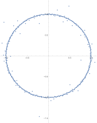
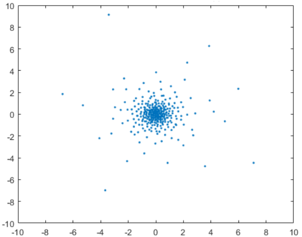
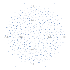
Figure 1: Roots of random polynomials A) Kac, B) Elliptic and C) Nearly Weyl, with complex Gaussian coefficients.

The jellium and zeros of random polynomials present very similar behaviors: for these two models, the sequence of empirical measures $(\mu_{n})_{n\in\mathbb{N}^{+}}$ converges towards $\nu$. Large deviation principles with speed $n^{2}$ but different rate functions are also valid. See [ZZ10, BZ17] for random polynomials and [Har12] for the jellium . At the microscopic level, zeros of random polynomials seem to differ, as it is suggested by the article of Krishnapur and Virag [KV14] which does not apply fully to this case. Figure 2 shows realizations of a jellium associated with the same measures $\nu$ as used in Figure 1: A) $\nu_{S^{1}}$ the uniform measure on the unit circle, B) $\nu_{FS}$ the Fubini-Study measure, and C) $\nu_{\mathbb{D}}$ the uniform measure on the unit disk.

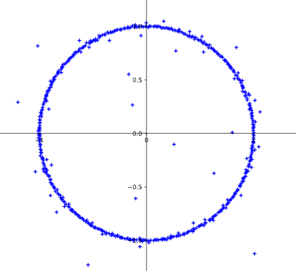
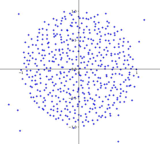
Figure 2: Jellium with background A) $\nu_{S^{1}}$, B) $\nu_{FS}$ et C) $\nu_{\mathbb{D}}$ .

1.2 Results on the jellium

In this section, we study the jellium. We are interested in the behavior of its extremals, i.e. either near the origin or near infinity. We prove that, near the origin, the point process formed by the jellium converges and its limit depends on the behavior of $\nu$ near the origin. A similar feature is observed near infinity. Outliers are seen to appear when $\nu$ gives zero charge to a neighborhood of the origin or to a neighborhood of infinity. These outliers will converge to a Bergman point process of a disk (neighborhood of zero) or of the complement of the disk (neighborhood of infinity) that we introduce now.

Definition 1.2 (Bergman point process).

The Bergman point process of an open set $U\subset\mathbb{C}$, written $\mathcal{B}_{U}$, is the determinantal point process on $U$ associated to the Bergman kernel of the set $U$. We will be interested in two particular cases: The case of an open disk $D_{R}$ of radius $R$ where the Bergman kernel is

$$\forall z,w\in D_{R}\quad K_{D_{R}}(z,w)=\frac{R^{2}}{\pi(R^{2}-z\bar{w})^{2}}$$

and the case of the complement of the closed disk of radius $R$ where the Bergman kernel is

$$\forall z,w\in\mathbb{C}\setminus\bar{D}_{R}\quad K_{\mathbb{C}\setminus\bar{D}_{R}}(z,w)=\frac{R^{2}}{\pi(R^{2}z\bar{w}-1)^{2}}.$$

For more information on the Bergman kernel, Bell [Bel15] gives a nice presentation on this topic. An interesting connection to random analytic functions is given in the work of Peres and Virág [PV05]. More specifically, they prove that $\mathcal{B}_{\mathbb{D}}$ can be seen as the zeros of a Gaussian analytic function. It can be shown that $\mathcal{B}_{\mathbb{D}}$ is invariant in law under any conformal map of $\mathbb{D}$ and that, almost surely, it has an infinite number of points and every point of the unit circle is an accumulation point of $\mathcal{B}_{\mathbb{D}}$.

Theorem 1.3 (Outliers for the jellium).

Let $\nu$ be a probability measure that satisfies Assumption 1 and let $(x_{1},\dots,x_{n})$ be a jellium associated to $\nu$. Let $U$ be a connected component of $\mathbb{C}\setminus\nolinebreak\mathrm{supp}\,\nu$ and suppose that it is either an open disk or the complement of a closed disk. Then the sequence of point processes $\{x_{k}\text{ such that }x_{k}\in U\}$ converges weakly as $n$ goes to infinity towards the Bergman point process $\mathcal{B}_{U}$ of $U$.

The topology on (deterministic) point process is reminded in the appendix, Section 5, for convenience of the reader. This theorem gives the universality of the outliers of the jellium since they only depend on the domain considered. In Figure 2, the outliers outside of the unit disk for a jellium associated to $\nu_{S^{1}}$ or $\nu_{\mathbb{D}}$ have the same limiting behavior.

If $\nu$ has compact support, the convergence of the point process outside a disk in Theorem 1.3 does not immediately imply the convergence of $\max_{k\in\{1,\dots,n\}}|x_{k}|$ towards a universal limiting random variable. Nevertheless, it can be obtained by an analysis of the minima in the inverted model and it is stated in the next corollary.

Corollary 1.4 (Particle of extremal modulus).

Let $\nu$ be a radial, compactly supported, probability measure satisfying Assumption 1. Let $R$ be the outer radius of the support of $\nu$. Then, we have

$$\max_{k\in\{1,\dots,n\}}|x_{k}|\xrightarrow[n\to\infty]{\rm{law}}R\,x_{\infty},$$

where $x_{\infty}$ is a random variable taking values in $[1,\infty)$ with cumulative distribution function

$$\mathbb{P}(x_{\infty}<t)=\prod_{k=1}^{\infty}\left(1-t^{-2k}\right).$$

The law of $R\,x_{\infty}$ is the same as the law of the maximum modulus of the Bergman point process of $\mathbb{C}\setminus\bar{D}_{R}$.

One can check that the random variable $x_{\infty}$ has a finite expected value but infinite variance, as well as the variable $\max_{k\in\{1,\dots,n\}}|x_{k}|$ for any $n$. This tells us that $\max_{k\in\{1,\dots,n\}}|x_{k}|$ is "often" far from $R$ as $n$ goes to infinity. This is a very different behavior from what was known in the context of strongly confining potentials [CP14], for which Gumbel fluctuations were established for the maximum of the modulus at the edge of the support.

Remark 1.5 (Universal behavior of the outer process and screening).

The limiting law of the modulus of the extremal particle and the limiting point process do not depend on the choice of background $\nu$. Since most of the particles fill the disk according to the measure $\nu$, the outer particles "see" two canceling effects: on the one hand they are attracted by the positive background, but they are repelled by the negative charges which have nearly the same effect as the background. The universal behavior of the outer point process is a consequence of this competition. Nevertheless, the behavior depends on the coefficient $(n+1)$ at the left side of $V$ on (1) as can be seen in [GZ19a].

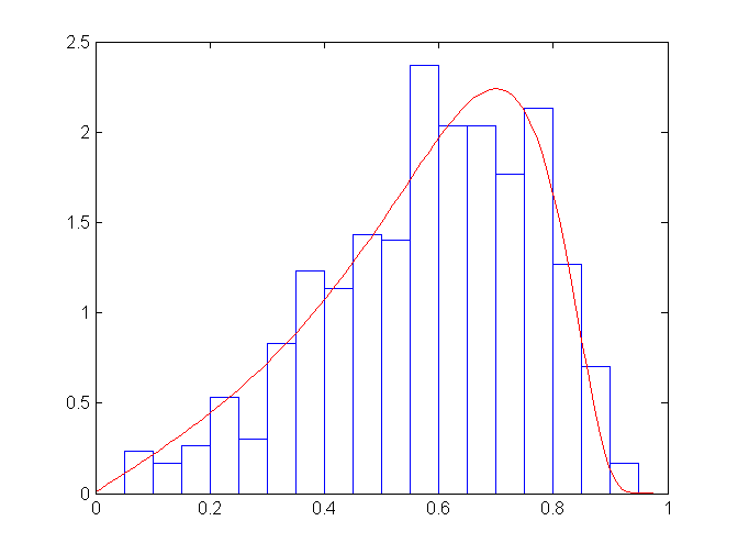
Figure 3: In blue: Histogram for the lowest modulus in a jellium associated to $\nu_{S^{1}}$ with $n=50$. In red: Density of the minimum modulus of $\mathcal{B}_{\mathbb{D}}$.

Figure 3 displays the histogram of a sample of $(\max_{k\in\{1,\dots,n\}}|x_{k}|)^{-1}$ for the jellium associated to the uniform measure on the unit circle, and the density of the minima of the Bergman point process of $\mathbb{D}$. Since $\max_{k\in\{1,\dots,n\}}|x_{k}|$ and its limit are heavy tailed, it was much more convenient to represent the convergence of their inverses.

Theorem 1.3 described the behavior of the extremal particles if the region is uncharged. The next theorem tells us what happens when the extremal region is no longer uncharged.

Theorem 1.6 (Extremal particles in the support).

Let $\nu$ be a measure that satisfies Assumption 1 and let $(x_{1},\dots,x_{n})$ be a jellium associated to $\nu$.

At the origin: Suppose there exists $\alpha>0$ and $\lambda>0$ such that

$$\lim_{r\to 0}\frac{\nu(D_{r})}{r^{\alpha}}=\lambda.$$

Then, $\{n^{1/\alpha}x_{1},\dots,n^{1/\alpha}x_{n}\}$ converges weakly towards the determinantal point process on $\mathbb{C}$ associated to the kernel

$$K(z,w)=\sum_{k=0}^{\infty}b_{k}z^{k}\bar{w}^{k}e^{-\gamma|z|^{\alpha}}e^{-\gamma|w|^{\alpha}}.$$ (7)

where

$$\gamma=\frac{\lambda}{\alpha}\,\,\mbox{ and }\,\,b_{k}^{-1}=2\pi\int_{0}^{\infty}r^{2k+1}e^{-2\gamma r^{\alpha}}{\rm d}r=2\pi\,\Gamma\left(\frac{2k+2}{\alpha}\right).$$

At infinity: Suppose there exists $\alpha>0$ and $\lambda>0$ such that

$$\lim_{r\to\infty}r^{\alpha}\nu(\hskip 0.5pt\mathbb{C}\setminus D_{r})=\lambda.$$ (8)

Then $\{n^{-1/\alpha}x_{1},\dots,n^{-1/\alpha}x_{n}\}$, considered as a point process on $\mathbb{C}\setminus\{0\}$, converges weakly towards the determinantal point process on $\mathbb{C}\setminus\{0\}$ associated to the kernel

$$K(z,w)=\sum_{k=0}^{\infty}\frac{b_{k}}{(z\bar{w})^{k+2}}e^{-\gamma|z|^{-\alpha}}e^{-\gamma|w|^{-\alpha}}$$

where

$$\gamma=\frac{\lambda}{\alpha}\,\,\mbox{ and }\,\,b_{k}^{-1}=2\pi\int_{0}^{\infty}r^{2k+1}e^{-2\gamma r^{\alpha}}{\rm d}r=2\pi\,\Gamma\left(\frac{2k+2}{\alpha}\right).$$

Convergence of the maximum: Under the same hypothesis (8), we have that

$$\frac{1}{n^{1/\alpha}}\max_{k\in\{1,\dots,n\}}|x_{k}|\xrightarrow[n\to\infty]{\mathrm{law}}\lambda^{1/\alpha}x_{\infty},$$

where $x_{\infty}$ is a random variable with cumulative distribution function

$$\mathbb{P}(x_{\infty}\leq t)=\prod_{k=1}^{\infty}\frac{\Gamma\left(\frac{2k}{\alpha},\frac{2}{\alpha t^{\alpha}}\right)}{\Gamma\left(\frac{2k}{\alpha}\right)}$$

and the $\Gamma$ with two arguments denotes the upper incomplete gamma function.

Theorem 1.6 extends the corresponding result of Jiang and Qi [JQ17, Theorem 1] on the spherical ensemble. Note that if $\nu$ has a positive density at the origin then the previous result applies with $\alpha=2$ and $\lambda$ equals to $\pi$ times the density at the origin. We recover the infinite Ginibre point process in that case. The main interest of the result is not the explicit limiting random variables but its universality and the fact that no further regularity is needed for $\nu$.

1.3 Results on random polynomials

In this section, we present results on the extremal zeros of random polynomials associated to a background measure $\nu$ which are the counterparts of the results obtained for the jellium in the previous section. The results are very close to what was obtained before and are presented in the same order.

Theorem 1.7 (Outliers for random polynomials).

Let $\nu$ be a probability measure satisfying Assumption 1 and let $z_{1},\dots,z_{n}$ be the zeros of a random polynomial $P_{n}$ (given by (5)) such that $a_{0}$ satisfies Assumption 2. Let $U$ be a connected component of $\mathbb{C}\setminus\nolinebreak\mathrm{supp}\,\nu$ and suppose that it is either an open disk or the complement of a closed disk.

Disk case: If $U=D_{R}$ for some $R>0$, then

$$\{z_{k}\text{ such that }z_{k}\in D_{R}\}\xrightarrow[n\to\infty]{\mathrm{law}}R\cdot\left\{z\in\mathbb{D}\text{ such that }\sum_{k=0}^{\infty}a_{k}z^{k}=0\right\}.$$

Complement of a disk case: If $U=\mathbb{C}\setminus\bar{D}_{R}$ for some $R>0$, then

$$\{z_{k}\text{ such that }z_{k}\in\mathbb{C}\setminus\bar{D}_{R}\}\xrightarrow[n\to\infty]{\mathrm{law}}R\cdot\left\{z\in\mathbb{C}\setminus\mathbb{D}\text{ such that }\sum_{k=0}^{\infty}a_{k}\frac{1}{z^{k}}=0\right\}.$$

Remark 1.8 (On the limiting random series).

Arnold [Arn66] showed that the random power series

$$\sum_{k=0}^{\infty}a_{k}z^{k}$$

has a radius of convergence equal to $1$ almost surely as soon as $\mathbb{E}(\log(1+|a_{0}|))<\infty$. In the specific case of complex Gaussian coefficients, Peres and Virág [PV05] showed that its zeros follow the same law as the Bergman point process of the unit disk. Hence, in the case of complex Gaussian coefficients, this result is exactly the same as the one for the jellium.

Corollary 1.9 (Zero of extremal modulus).

Let $\nu$ be a probability measure satisfying Assumption 1 and let $z_{1},\dots,z_{n}$ be the zeros of a random polynomial $P_{n}$ (given by (5)) such that $a_{0}$ satisfies Assumption 2. Let $R$ be the outer radius of the support of $\nu$, then

$$\max_{k\in\{1,\dots,n\}}|z_{k}|\xrightarrow[n\to\infty]{\mathrm{law}}R\,\max\left\{|z|\text{ such that }z\in\mathbb{C}\setminus\mathbb{D}\mbox{ and }\sum_{k=0}^{\infty}a_{k}\frac{1}{z^{k}}=0\right\}.$$

In particular, if $a_{0}$ is a complex Gaussian random variable, we have

$$\max_{k\in\{1,\dots,n\}}|z_{k}|\xrightarrow[n\to\infty]{\rm{law}}R\,z_{\infty},$$

where $z_{\infty}$ is a random variable taking values in $[1,\infty)$ with cumulative distribution function

$$\mathbb{P}(z_{\infty}<t)=\prod_{k=1}^{\infty}\left(1-t^{-2k}\right).$$

The limiting random variable that appears in the corollary is only explicitly known for complex Gaussian coefficients, where it is the maximum modulus of the Bergman point process of $D_{R}$, as in Corollary 1.4. For general coefficients, this random variable, as well as $\max_{k\in\{1,\dots,n\}}|z_{k}|$ are heavy tailed [But18]. More precisely, if

$$\varliminf_{t\to 0^{+}}t^{-m}\mathbb{P}(|a_{0}|<t)>0,$$

then the $m$-th moment of $\max_{k\in\{1,\dots,n\}}|z_{k}|$ as well as the $m$-th moment of its limit are infinite. Figure 4 illustrates the convergence of $(\max_{k\in\{1,\dots,n\}}|z_{k}|)^{-1}$ for Gaussian Kac polynomials (i.e. when $\nu=\nu_{S^{1}}$ and $a_{0}$ is a complex Gaussian random variable) towards the minimum modulus of the Bergman point process.

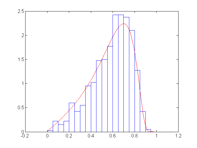
Figure 4: In blue: Histogram for the inverse of the largest root in modulus of Kac polynomials with complex Gaussian coefficients for $n=200$. In red: Density of the minimum modulus of the Bergman point process of $\mathbb{D}$.

In the case where the support of $\nu$ is unbounded or contains the origin, we observe a phenomenon similar to the results of Theorem 1.6 but for which the limiting random variable differs from the jellium case.

Theorem 1.10 (Rescaled extremal roots of random polynomials).

Let $\nu$ be a measure satisfying Assumption 1 and let $z_{1},\dots,z_{n}$ be the zeros of a random polynomial $P_{n}$ (given by (5)) such that $a_{0}$ satisfies Assumption 2.

At the origin: If there exists $\alpha>0$ and $\lambda>0$ such that

$$\lim_{r\to 0}\frac{\nu(D_{r})}{r^{\alpha}}=\lambda$$ (9)

then the point process $\{n^{1/\alpha}z_{1},\dots,n^{1/\alpha}z_{n}\}$ converges almost surely towards the roots of the following random entire function

$$f_{\alpha,\lambda}(z)=\sum_{k=0}^{\infty}\frac{a_{k}}{\Gamma(1+\frac{2k}{\alpha})^{1/2}}\left(\frac{\lambda}{\alpha}\right)^{k/\alpha}z^{k},$$

sometimes known as the Mittag-Leffler random function.

At infinity: If there exists $\alpha>0$ and $\lambda>0$ such that

$$\lim_{r\to\infty}r^{\alpha}\nu\,(\hskip 0.5pt\mathbb{C}\setminus D_{r})=\lambda$$ (10)

then the point process $\{n^{-1/\alpha}z_{1},\dots,n^{-1/\alpha}z_{n}\}$, seen as a point process on $\mathbb{C}\setminus\{0\}$, converges in law towards the inverse of the point process of the zeros of $f_{\alpha,\lambda}$.

Convergence of the maximum: Under the same hypothesis (10), we also have

$$\frac{1}{n^{1/\alpha}}\max_{k\in\{1,\dots,n\}}|z_{k}|\xrightarrow[n\to\infty]{\mathrm{law}}\max\{|z|\text{ such that }z\in\mathbb{C}\setminus\{0\}\mbox{ and }f_{\alpha,\lambda}(1/z)=0\}.$$

When $\alpha=2$ and $\lambda=2$, which occurs for elliptic polynomials, we have

$$f_{2,2}(z)=\sum_{k=0}^{\infty}a_{k}\frac{1}{\sqrt{k!}}z^{k}.$$

and, if $a_{0}$ is a complex standard Gaussian random variable, this random function is known as the planar Gaussian Analytic function. For different $\alpha$ and $\lambda$ but still complex Gaussian coefficients, the random Mittag-Leffler functions are studied for the rigidity of their zero set [KN19].

Remark 1.11.

In the special case $\nu=\nu_{S^{1}}$, the uniform measure on the unit circle, Theorem 1.7 and Corollary 1.9 are just a direct consequence of the result of Arnold [Arn66], while the identification of the limiting point process for complex Gaussian coefficients is exactly the result of Peres and Virág [PV05]. For all the other models of random polynomials, our result is new. There is no hope to observe the Bergman point process for non-Gaussian coefficients, as it was already noticed in [TV15, Section 5]. See [But18] for a discussion of this non-universality in the case of the Kac polynomials.

It is possible to extend Theorem 1.7 to the case where $\nu(\mathbb{C})>1$. Indeed, the same methods that will be used to prove Theorem 1.7 would allow us to prove the straightforward generalization. Since it escapes the main models of interest in this article, we will only state the case of Weyl polynomials which have an easier and shorter proof.

Theorem 1.12 (Extremal particles for the Weyl polynomials).

Let $(a_{k})_{k\in\mathbb{N}}$ be a sequence of i.i.d. random variables satisfying Assumption 2. Let

$$P_{n}(z)=\sum_{k=0}^{n}\frac{\sqrt{n^{k}}}{\sqrt{k!}}a_{k}z^{k}.$$

If $z_{1},\dots,z_{n}$ are the zeros of $P_{n}$ then

$$\{z_{k}\text{ such that }|z_{k}|>1\}\xrightarrow[n\to\infty]{\mathrm{law}}\left\{z\in\mathbb{C}\setminus\bar{\mathbb{D}}\text{ such that }\sum_{k=0}^{\infty}a_{k}\frac{1}{z^{k}}=0\right\}.$$

Furthermore, we have the convergence of the maxima. In particular, when $a_{0}$ is a complex Gaussian random variable, for every $t\in[1,\infty)$ we have

$$\lim_{n\to\infty}\mathbb{P}(\max\{|z|:P_{n}(z)=0\}\leq t)=\prod_{k=1}^{\infty}\left(1-t^{-2k}\right).$$

1.4 Symmetries of the models

The jellium and the zeros of random polynomials have a lot of symmetries, which make those models particularly interesting to study. The jellium, as well as the roots of random polynomials, are stable under the inversion map $i:\mathbb{C}\setminus\{0\}\to\mathbb{C}\setminus\{0\}$, given by

$$i(z)=\frac{1}{z},$$

and also by scaling. This means that under these transformations, a jellium associated to $\nu$ has the same law as a jellium associated to another measure $\nu^{\prime}$. The same is true for zeros of random polynomials.

Theorem 1.13 (Equivariance of the jellium).

Let $\nu$ be a probability measure satisfying Assumption 1 and let $(x_{1},\dots,x_{n})$ be a jellium associated to $\nu$. Then, for any $\lambda>0$, $(\lambda x_{1},\dots,\lambda x_{n})$ has the law of a jellium associated to $\nu(\cdot/\lambda)$ and $(i(x_{1}),\dots,i(x_{n}))$ has the law of a jellium associated to $i_{*}\nu$, the pushforward of $\nu$ by $i$.

The pushforward $i_{*}\nu$ is well-defined since the measure $\nu$ has no atom at $0$ due to Assumption 1. Furthermore, $(i(x_{1}),\dots,i(x_{n}))$ is well-defined almost surely because the event $\{\exists k\text{ such that }x_{k}=0\}$ has zero probability so that the statement of Theorem 1.13 makes sense.

Theorem 1.14 (Equivariance of the zeros of random polynomials).

Let $\nu$ be a probability measure satisfying Assumption 1 and let $z_{1},\dots,z_{n}$ be the zeros of a random polynomial (given by (5)) associated to some i.i.d. sequence $(a_{k})_{k\in\{0,\dots,n\}}$. Then, for every $\lambda>0$, the point process formed by $\lambda z_{1},\dots,\lambda z_{n}$ has the same law as the one formed by the zeros of the random polynomial associated to $\nu(\cdot/\lambda)$ and to the same sequence $(a_{k})_{k\in\{0,\dots,n\}}$. In addition, the point process formed by $i(z_{1}),\dots,i(z_{n})$ has the same law as the one formed by the zeros of the random polynomial associated to $i_{*}\nu$, the pushforward of $\nu$ by $i$, and to the same sequence $(a_{k})_{k\in\{0,\dots,n\}}$.

Remark 1.15 (Equivariance under Möbius transformations).

If we allow non-radial $\nu$, the jellium is also equivariant under translations. This implies the equivariance of the jellium with respect to all Möbius transformations. Zeros of random polynomials with complex Gaussian coefficients are also equivariant under translations, hence under all Möbius transformations. For general coefficients and non-radial measures $\nu$, the model of random polynomials depends on the choice of basis and this basis would have to be transformed accordingly for the equivariance to hold.

The next result is standard and it is contained, for instance, in [HKPV09, Section 5.4] where a connection to Gaussian analytic functions is made. It follows from the equivariance of the Bergman kernel together with the change of variables formula in Lemma 5.3.

Theorem 1.16 (The Bergman point process is conformally invariant).

Let $U_{1}$ and $U_{2}$ be open sets in $\mathbb{C}$ and suppose that there exists a biholomorphism $\varphi$ from $U_{1}$ to $U_{2}$. Then,

$$\varphi(\mathcal{B}_{U_{1}})\overset{\rm law}{=}\mathcal{B}_{U_{2}}.$$

These theorems combined together allow us to reduce the proofs to the study of the point processes near the origin.

Remark 1.17 (On the disk and the complement of a disk).

Notice that the Bergman kernel of $D_{R}\setminus\{0\}$ is the restriction of the Bergman kernel of $D_{R}$ since a square integrable singularity is a removable singularity. This implies that the restriction of $\mathcal{B}_{D_{R}}$ to $D_{R}\setminus\{0\}$ is $\mathcal{B}_{D_{R}\setminus\{0\}}$. In particular, by applying Theorem 1.16, we can say that

$$i(\mathcal{B}_{D_{R}})\overset{\rm law}{=}\mathcal{B}_{\mathbb{C}\setminus\bar{D}_{R}}$$

where $i(\mathcal{B}_{D_{R}})$ makes sense since $0\notin\mathcal{B}_{D_{R}}$ almost surely or, strictly speaking, $i(\mathcal{B}_{D_{R}})$ means the inverse of the restriction of $\mathcal{B}_{D_{R}}$ to $D_{R}\setminus\{0\}$. This can also be obtained by using the explicit formulas given in Definition 1.2.

2 Comments and perspectives

2.1 Related results

A nice introduction to the theory of Coulomb gases can be found in [Ser18]. Coulomb gases are usually studied for strongly confining potentials. [Rid03] showed that the particles of a Ginibre ensemble converge towards the closed unit disk and that the particle farthest from zero exhibits Gumbel fluctuations. This result has been further generalized and different cases have been found in [CP14, Seo15, JQ17, CLQ18, GQ18, LACTGMS18, GZ19a, CGZJ20], always in the radial determinantal setting. Very recently, [Ame19] showed a control of the distance between the particles and the support of the equilibrium measure for general temperatures and not necessarily radial potentials.

A universal limit point process at a point in the bulk where the equilibrium measure has a positive density has been established, for instance, in [Ber13]. Further behaviors in the bulk are studied in [AS18, AKS18, GZ19a] and a nice condition has been given for a radial case in Theorem 1.6 where the regularity outside the origin is not needed. Limiting point process at the edge have been found in [Ame18, AKM19, HW19, GZ19a, AKS19]. To our knowledge, this is the first time that the limiting behavior of the point process for weakly confining potentials has been studied outside the bulk.

2.2 Open questions

For non-radial measures $\nu$ at inverse temperature $2$, we expect our results to generalize: for any connected component $U$ of $\mathbb{C}\setminus\text{supp }\nu$, simply connected, the outliers should converge towards the Bergman point process $\mathcal{B}_{U}$ in the jellium case as well as in the case of the zeros of random polynomials with complex Gaussian coefficients. For general coefficients, for a good choice of basis, we expect to see the zeros of a random function of the form

$$z\mapsto\sum_{k=0}^{\infty}a_{k}\varphi(z)^{k}$$

where $\varphi$ is a conformal map from $U$ to the unit disk.

If we do not assume that the inverse temperature is $2$, all the results presented in this article fall. We hope that similar results hold for any inverse temperature $\beta$. In dimension one, the Sine point process and the Airy point process have $\beta$ counterparts which generalizes them to any temperature. See [VV09] and [RRV11]. We can dream of a generalization to any $\beta$ of the Bergman point process.

For random polynomials, the study of the outliers in the case where $\nu$ is not radial seems hard to study. One may try to understand the behavior of the orthogonal polynomials $R_{k,n}$ associated to an inner product

$$\langle P,Q\rangle_{n,\nu}=\int P(z)\overline{Q(z)}e^{-2nV^{\nu}(z)}{\rm d}\nu(z)$$

which is in general a difficult question. After it is understood, the study of the outliers could be carried out by studying the asymptotics of the covariance kernel of the Gaussian field $(P_{n}(z))_{z\in\mathbb{C}}$

$$K_{n}(z,w)=\sum_{k=0}^{n}R_{k,n}(z)\overline{R_{k,n}(w)}$$

outside of the support of $\nu$.

3 Proof of the equivariance results

We start by proving the equivariance for the jellium, then for the zeros of random polynomials and finally for the Bergman point processes. We remark that these theorems and their proofs are geometric in nature and that they can be nicely explained by using the language of complex line bundles on a regular setting.

Proof of Theorem 1.13.

The equivariance under scaling is straightforward. We only prove the equivariance with respect to the inversion. Let $(x_{1},\dots,x_{n})$ be a jellium associated to a probability measure $\nu$ satisfying Assumption 1. This means that it follows the law

$$\frac{1}{Z_{n}}\exp\left(-2\left[-\sum_{i<j}\log|x_{i}-x_{j}|+(n+1)\sum_{i=1}^{n}V^{\nu}(x_{i})\right]\right){\rm d}\ell_{\mathbb{C}^{n}}(x_{1},\dots,x_{n})$$ (11)

where $Z_{n}$ is a normalization constant. Define

$$G^{V^{\nu}}(x,y)=-\log|x-y|+V^{\nu}(x)+V^{\nu}(y)$$

and define the positive measure $\pi$ by ${\rm d}\pi=e^{-4V^{\nu}}{\rm d}\ell_{\mathbb{C}}$. Using these definitions we can write

$$\exp \left(-2\left[-\sum_{i<j}\log|x_{i}-x_{j}|+(n+1)\sum_{i=1}^{n}V^{\nu}(x_{i})\right]\right){\rm d}\ell_{\mathbb{C}^{n}}(x_{1},\dots,x_{n})$$

$$=\exp\left(-2\sum_{i<j}G^{V^{\nu}}(x_{i},x_{j})\right){\rm d}\pi^{\otimes_{n}}(x_{1},\dots x_{n}).$$ (12)

We define the function $\tilde{V}$ as

$$\tilde{V}(z)={V^{\nu}}\left(\frac{1}{z}\right)+\log|z|.$$

By a straightforward calculation, we obtain that

$$G^{V^{\nu}}(i(x),i(y))=-\log|x-y|+\tilde{V}(x)+\tilde{V}(y)=:G^{\tilde{V}}(x,y)$$

and that $\tilde{\pi}:=i_{*}\pi$ (the pushforward measure of $\pi$ by $i$) is given by

$${\rm d}\tilde{\pi}=e^{-4\tilde{V}}{\rm d}\ell_{\mathbb{C}}.$$

In summary, the ‘inverse’ of $e^{-2\sum_{i<j}G^{V^{\nu}}(x_{i},x_{j})}$ is $e^{-2\sum_{i<j}G^{\tilde{V}}(x_{i},x_{j})}$ and the ‘inverse’ of $\pi$ is $\tilde{\pi}$ so that the inverse of (12) is

$$\exp\left(-2\sum_{i<j}G^{\tilde{V}}(x_{i},x_{j})\right)\mathrm{d}\tilde{\pi}^{\otimes_{n}}(x_{1},\dots,x_{n})$$

$$\quad\quad\quad=\exp\left(-2\left[-\sum_{i<j}\log|x_{i}-x_{j}|+(n+1)\sum_{i=1}^{n}\tilde{V}(x_{i})\right]\right){\rm d}\ell_{\mathbb{C}^{n}}(x_{1},\dots,x_{n}).$$

We finish the proof of the theorem by noticing that

$$\forall z\in\mathbb{C}\setminus\{0\},\quad V^{i_{*}\nu}(z)=V^{\nu}\left(\frac{1}{z}\right)+\log|z|-V^{\nu}(0).$$

Hence, $\tilde{V}$ differs from $V^{i_{*}\nu}$ by a constant. One can remove the constant $V^{\nu}(0)$ from the definition of the potential as it may enter into the normalizing constant associated to this model. ∎

Proof of Theorem 1.14.

The equivariance under scaling is a straightforward calculation. For the inversion, let $P_{n}$ be given by (5) associated to $\nu$ and to an i.i.d. sequence $(a_{k})_{k\in\{1,\dots,n\}}$. We show that the random polynomial $Q_{n}$ defined by

$$Q_{n}(z)=z^{n}P_{n}\left(\frac{1}{z}\right)$$

has the same law as the one given by $(5)$ associated to the measure $i_{*}\nu$ and to the same sequence $(a_{k})_{k\in\{1,\dots,n\}}$.

By a change of variables formula, it can be seen that the application ${}^{*}:\mathbb{C}_{n}[X]\to\mathbb{C}_{n}[X]$ that to each polynomial $P\in\mathbb{C}_{n}[X]$ associates the polynomial $P^{*}\in\mathbb{C}_{n}[X]$ given by

$$P^{*}(z)=z^{n}P(1/z)$$

is an isometry between $\mathbb{C}_{n}[X]$ with the inner product defined by

$$\langle P,Q\rangle_{n,\nu}=\int_{\mathbb{C}}P\overline{Q}e^{-2nV^{\nu}}{\rm d}\nu$$

and $\mathbb{C}_{n}[X]$ with the inner product defined by

$$\langle P,Q\rangle_{n,i_{*}\nu}=\int_{\mathbb{C}}P\overline{Q}e^{-2nV^{i_{*}\nu}}di_{*}\nu.$$

By also noticing that $*$ preserves the monomials, needed only in the general non-Gaussian case, the proof is completed. ∎

Proof of Theorem 1.16.

We start by recalling an important relation satisfied by Bergman kernels on different open sets. Let $U_{1}$ and $U_{2}$ be two open sets and $\varphi$ be a biholomorphism from $U_{1}$ to $U_{2}$. Then, if $K_{U_{1}}$ is the Bergman kernel of $U_{1}$ and $K_{U_{2}}$ is the Bergman kernel of $U_{2}$, we have, by [Bel15, Theorem 16.5],

$$\forall z,w\in U_{1}\quad K_{U_{1}}(z,w)=\varphi^{\prime}(z)K_{U_{2}}(\varphi(z),\varphi(w))\overline{\varphi^{\prime}(w)}.$$

We conclude by an application of the change of variables formula for determinantal point processes given in Lemma 5.3.

∎

4 Proof of the main results

We start by proving a key lemma which will be essential in several of the proofs. It gives a very tractable formula for the potential of radial measures.

Lemma 4.1 (Useful formula for the potential).

Let $\nu\in\mathcal{P}(\mathbb{C})$ be a rotationally invariant probability measure such that $\int_{\mathbb{C}\setminus\mathbb{D}}\log|x|{\rm d}\nu(x)<\infty$. Then

$$V^{\nu}(z)=\int_{1}^{|z|}\frac{\nu(D_{r})}{r}{\rm d}r+\int_{\mathbb{C}\setminus\mathbb{D}}\log|x|{\rm d}\nu(x)$$

where $D_{r}$ denotes the open disk of radius $r$.

This formula is standard and can be seen to be related to Poisson-Jensen formula [ST97, Theorem II.4.10].

Remark 4.2 (The potential is defined up to a constant.).

We recall that one can choose to add a constant to the potential $V^{\nu}$ without changing the law (1). Adding a constant will only change the normalizing constant $Z_{N}$. The potential $V^{\nu}$ can be modified so that it is equal to zero at the unit circle and then

$$\forall z\in\mathbb{C}\quad V^{\nu}(z)=\int_{1}^{|z|}\frac{\nu(D_{r})}{r}{\rm d}r.$$

In fact, $V^{\nu}$ defined in this way satisfies Poisson’s equation with source $2\pi\nu$ even if the actual logarithmic potential (4) does not make sense. Nevertheless, it is only when the condition of Lemma 4.1 is satisfied that $V^{\nu}$ satisfies condition (3). We emphasize again that this representation of the potential will be very helpful in the rest of the article.

Proof of Lemma 4.1.

Since $\nu$ is radial, the disintegration theorem [AGS08, Theorem 5.3.1] allows us to write

$$\nu=\int_{0}^{\infty}l_{r}{\rm d}\mu(r)$$

where $l_{r}\in\mathcal{P}(\mathbb{C})$ is the uniform probability measure on $C_{r}$, the circle centered at $0$ of radius $r$, and $\mu$ is a probability measure on $[0,\infty)$ characterized by

$$\forall a,b>0\quad\mu((a,b))=\nu(\{a<|z|<b\}).$$

This decomposition of the measure means that for any $f$ positive measurable function or integrable with respect to $\nu$ we have

$$\int_{\mathbb{C}}f(z){\rm d}\nu(z)=\int_{0}^{\infty}\left(\int_{C_{r}}f(w)dl_{r}(w)\right){\rm d}\mu(r).$$

Using this relation to compute the potential of the measure $\nu$ we have that for every $z\in\mathbb{C}$

$$V^{\nu}(z)=\int_{\mathbb{C}}\log|z-w|{\rm d}\nu(w)= \int_{0}^{\infty}\left(\int_{C_{r}}\log|z-w|dl_{r}(w)\right){\rm d}\mu(r)$$

$$= \int_{0}^{\infty}V^{l_{r}}(z){\rm d}\mu(r).$$

where $V^{l_{r}}$ is the potential of the uniform measure on $C_{r}$. In fact, since the integrability of $\log|z-\cdot|$ is not yet known we may proceed by a limiting argument by first integrating over the complement of an open annulus that contains $z$. But, since $V^{l_{r}}$ can be computed explicitly and is equal to [Ran95, p.29]

$$V^{l_{r}}(z)=\begin{cases}\log r&\text{ if }|z|\leq r\\ \log|z|&\text{ if }|z|>r\end{cases}$$

we are able to complete the limiting argument. Hence we obtain

$$V^{\nu}(z) =\int_{[|z|,\infty)}\log r\,{\rm d}\mu(r)+\int_{[0,|z|)}\log|z|{\rm d}\mu(r)$$

$$=\int_{[|z|,\infty)}\log r\,{\rm d}\mu(r)+\log|z|\nu(D_{|z|})$$ (13)

where the last term is not there if $z=0$. Notice that, by (13), the lemma is already proven for $|z|=1$. Suppose that $z\neq 0$. Let us notice that Fubini’s theorem implies

$$\int_{|z|}^{\infty}\frac{1}{r}\nu(\hskip 0.5pt\mathbb{C}\setminus D_{r}){\rm d}r =\int_{\mathbb{R}^{+}}1_{r\geq|z|}\frac{1}{r}\left(\int_{\mathbb{R}^{+}}1_{s\geq r}{\rm d}\mu(s)\right){\rm d}r$$

$$=\int_{\mathbb{R}^{+}}1_{s\geq|z|}\left(\int_{|z|}^{s}\frac{1}{r}{\rm d}r\right)\,{\rm d}\mu(s)$$

$$=\int_{[|z|,\infty)}\log s\,{\rm d}\mu(s)-\log|z|\nu(\hskip 0.5pt\mathbb{C}\setminus D_{|z|}).$$

Then, by replacing this equality in (13), we obtain

$$V^{\nu}(z) =\log|z|\left[\,\nu(D_{|z|})+\nu(\hskip 0.5pt\mathbb{C}\setminus D_{|z|})\,\right]+\int_{|z|}^{\infty}\frac{\nu(\hskip 0.5pt\mathbb{C}\setminus D_{r})}{r}{\rm d}r$$

$$=\log|z|+\int_{|z|}^{1}\frac{\nu(\hskip 0.5pt\mathbb{C}\setminus D_{r})}{r}{\rm d}r+\int_{1}^{\infty}\frac{\nu(\hskip 0.5pt\mathbb{C}\setminus D_{r})}{r}{\rm d}r$$

$$=\log|z|+\int_{|z|}^{1}\frac{1-\nu(D_{r})}{r}{\rm d}r+\int_{1}^{\infty}\frac{\nu(\hskip 0.5pt\mathbb{C}\setminus D_{r})}{r}{\rm d}r$$

$$=\int_{1}^{|z|}\frac{\nu(D_{r})}{r}{\rm d}r+\int_{1}^{\infty}\frac{\nu(\hskip 0.5pt\mathbb{C}\setminus D_{r})}{r}{\rm d}r$$

$$=\int_{1}^{|z|}\frac{\nu(D_{r})}{r}{\rm d}r+\int_{[1,\infty)}\log r\,{\rm d}\mu(r)$$

where the last equality is obtained by taking $|z|=1$. The case $z=0$ follows the same argument.

∎

4.1 Results for the jellium

4.1.1 Proof of Theorem 1.3

Proof of Theorem 1.3.

Due to the equivariance of the jellium, stated in Theorem 1.13, and the equivariance of the Bergman point process from Theorem (1.16) together with Remark 1.17, it suffices to assume that $U$, the connected component of $\mathbb{C}\setminus\text{supp }\nu$, is the open unit disk, which can be written as

$$S^{1}\subset\mathrm{supp}\,\nu\subset\mathbb{C}\setminus\mathbb{D}.$$

Step 1: Kernel of the Coulomb gas

Let $\nu$ be a measure satisfying Assumption 1 such that $S^{1}\subset\mathrm{supp}\,\nu\subset\mathbb{C}\setminus\mathbb{D}$. Let $(x_{1},\dots,x_{n})$ be a jellium associated to $\nu$. Notice that, due to Lemma 4.1, $V^{\nu}$ is constant in the unit disk, which we set to be equal to $0$ (see Remark 4.2). The point process $\{x_{1},\dots,x_{n}\}$ is determinantal, because it is a Coulomb gas in the plane with inverse temperature $2$. It is associated to the kernel $K_{n}:\mathbb{C}\times\mathbb{C}\to\mathbb{C}$ defined by

$$K_{n}(z,w)=\sum_{k=0}^{n-1}b_{k,n}z^{k}\bar{w}^{k}e^{-(n+1)V^{\nu}(z)}e^{-(n+1)V^{\nu}(w)}$$

where

$$(b_{k,n})^{-1}=\int_{\mathbb{C}}|z|^{2k}e^{-2(n+1)V^{\nu}(z)}{\rm d}\ell_{\mathbb{C}}(z).$$

The point process $\mathcal{I}_{n}=\{x_{k}:|x_{k}|<1\}$ is the restriction to the open unit disk of the point process $\{x_{1},\dots,x_{n}\}$, and is also a determinantal point process, with kernel given by the restriction of $K_{n}$ to $\mathbb{D}\times\mathbb{D}$. We will also denote this kernel by $K_{n}$. By [ST03, Proposition 3.10], stated in Proposition 5.4 for convenience, in order to prove the convergence of the sequence of point processes $(\mathcal{I}_{n})_{n\in\mathbb{N}^{+}}$ towards the Bergman point process of $\mathbb{D}$, it is enough to prove that the sequence of kernels $(K_{n})_{n\in\mathbb{N}^{+}}$ converges uniformly on compact subsets of $\mathbb{D}\times\mathbb{D}$ towards

$$K(z,w)=\frac{1}{\pi}\frac{1}{(1-z\bar{w})^{2}}=\sum_{k=0}^{\infty}\frac{k+1}{\pi}z^{k}\bar{w}^{k}.$$

In fact, the proof will work, and thus the theorem is true, as soon as the radial potential $V$ satisfying (3) is zero inside of the closed unit disk and positive outside of it.

Step 2: Convergence of the coefficients

First, let us notice that

$$(b_{k,n})^{-1} =\int_{\mathbb{C}}|z|^{2k}e^{-2(n+1)V^{\nu}(z)}{\rm d}\ell_{\mathbb{C}}(z)=2\pi\int_{0}^{\infty}r^{2k+1}e^{-2(n+1)V^{\nu}(r)}{\rm d}r$$

$$=2\pi\int_{0}^{1}r^{2k+1}e^{-2(n+1)V^{\nu}(r)}{\rm d}r+2\pi\int_{1}^{\infty}r^{2k+1}e^{-2(n+1)V^{\nu}(r)}{\rm d}r,$$

where we use $V^{\nu}(r)$ to denote $V^{\nu}$ evaluated at any point of norm $r$. Since the potential $V^{\nu}$ is equal to $0$ inside the unit disk, one can compute the first term

$$2\pi\int_{0}^{1}r^{2k+1}e^{-2(n+1)V(r)}{\rm d}r=2\pi\int_{0}^{1}r^{2k+1}{\rm d}r=\frac{\pi}{k+1}.$$

For the second term, let us prove that

$$\lim_{n\to\infty}\int_{1}^{\infty}r^{2k+1}e^{-2(n+1)V^{\nu}(r)}{\rm d}r=0.$$

But this is a consequence of Lebesgue’s dominated convergence theorem where we use the bound

$$r^{2k+1}e^{-2(n+1)V^{\nu}(r)}\leq r^{2k+1}e^{-2(k+2)V^{\nu}(r)}$$

for $k\leq n-1$. The fact that $r^{2k+1}e^{-2(n+1)V^{\nu}(r)}$ goes to zero when $r>1$ can be seen from the fact that $V^{\nu}(r)>0$ which in turn can be seen from the formula in Lemma 4.1 as follows. Let $r>1$ and write

$$V^{\nu}(r)=\int_{1}^{r}\frac{\nu(D_{s})}{s}{\rm d}s.$$

If $V^{\nu}(r)$ were zero the integrand $\nu(D_{s})$ would be zero for almost every $s\in[1,r]$ which is impossible because $\nu(D_{s})>0$ for $s>1$.

In summary, we obtain $\lim_{n\to\infty}b_{k,n}=\frac{k+1}{\pi}.$

Step 3: Convergence of the kernels

Let us fix $\rho\in(0,1)$ then for any $z$, $w$ inside the disk of radius $\rho$ we have

$$|K_{n}(z,w)-K(z,w)|\leq\sum_{k=0}^{\infty}\left|b_{k,n}-\frac{k+1}{\pi}\right||z|^{k}|w|^{k}\leq\sum_{k=0}^{\infty}\left|b_{k,n}-\frac{k+1}{\pi}\right|\rho^{2k}.$$

The right-hand term converges to zero as $n$ goes to infinity by an application of Lebesgue’s dominated convergence theorem, noticing that

$$\forall k,n\quad 0\leq b_{k,n}\leq\frac{k+1}{\pi}.$$

which implies

$$\left|b_{k,n}-\frac{k+1}{\pi}\right|\rho^{2k}\leq 2\left(\frac{k+1}{\pi}\right)\rho^{2k}.$$

By [ST03, Proposition 3.10] the point process $\mathcal{I}_{n}$ converges towards the Bergman point process $\mathcal{B}_{\mathbb{D}}$. ∎

Proof of Corollary 1.4.

In the case where $U$ is the open unit disk, the point process of the outliers $\mathcal{I}_{n}$ converges towards $\mathcal{B}_{\mathbb{D}}$. By the continuity of the minimum (Lemma 5.1 in the appendix) we obtain that the minimum of the norms of $\mathcal{I}_{n}$ converges to the minimum of the norms of $B_{\mathbb{D}}$. But the limit of the minimum of the norms of $\mathcal{I}_{n}$ coincides with the limit of the minimum of $\{|x_{1}|,\dots,|x_{n}|\}$ since the latter limit is bounded by $1$.

Thanks to [HKPV09, Theorem 4.7.1], the set of norms of the Bergman point process of $\mathbb{D}$ has the same law as $\{U_{k}^{1/2k},k\in\mathbb{N}\setminus\{0\}\}$, with the ${U_{k}}^{\prime}s$ being independent uniform random variables on $[0,1)$. This immediately implies that

$$\mathbb{P}\left(\,\inf\{|z|:z\in\mathcal{B}_{\mathbb{D}}\}\leq t\right)=1-\prod_{k=0}^{\infty}(1-t^{2k}).$$

We conclude the proof by applying the inversion and a scaling. ∎

4.1.2 Proof of Theorem 1.6

Proof.

We prove the first part of the theorem, and we deduce the rest thanks to the equivariance under inversion of the jellium.

Proof at the origin.

Step 1: Kernel of the rescaled Coulomb gas

Let $(x_{1},\dots,x_{n})$ be a jellium associated to $\nu$. Then the point process $\left\{\frac{x_{1}}{n^{1/\alpha}},\dots,\frac{x_{n}}{n^{1/\alpha}}\right\}$ is a determinantal point process associated to the kernel

$$\tilde{K}_{n}(z,w) =\frac{1}{n^{2/\alpha}}K_{n}\left(\frac{z}{n^{1/\alpha}},\frac{w}{n^{1/\alpha}}\right)$$

$$=\sum_{k=0}^{n}b_{k,n}z^{k}\bar{w}^{k}e^{-(n+1)V^{\nu}\left(\frac{z}{n^{1/\alpha}}\right)}e^{-(n+1)V^{\nu}\left(\frac{w}{n^{1/\alpha}}\right)}$$

where

$$b_{k,n}^{-1}=2\pi\int_{0}^{\infty}r^{2k+1}e^{-2(n+1)V^{\nu}\left(\frac{r}{n^{1/\alpha}}\right)}{\rm d}r.$$

This may be seen, for instance, by the change of variables formula in Lemma 5.3. We will prove that the sequence of kernels $(\tilde{K}_{n})_{n\in\mathbb{N}}$ converges uniformly on compact subsets of $\mathbb{C}\times\mathbb{C}$ towards the kernel

$$K(z,w)=\sum_{k=0}^{\infty}b_{k}z^{k}\bar{w}^{k}e^{-\gamma|z|^{\alpha}}e^{-\gamma|w|^{\alpha}}$$ (14)

where

$$\gamma=\frac{\lambda}{\alpha}\,\,\mbox{ and }\,\,b_{k}^{-1}=2\pi\int_{0}^{\infty}r^{2k+1}e^{-2\gamma r^{\alpha}}{\rm d}r.$$

To prove this convergence, we will first prove that $\lim_{n\to\infty}b_{k,n}=b_{k}$, then we will find a sequence $(B_{k})_{k\in\mathbb{N}}$ such that $\sum_{k=0}^{\infty}B_{k}r^{k}$ has an infinite radius of convergence and $b_{k,n}\leq B_{k}$ for every $n$. This will imply the uniform convergence of the kernels.

Step 2: Properties satisfied by the potential

Let $\nu$ be a rotationally invariant probability measure such that there exists $\alpha>0$ and $\lambda>0$ with

$$\lim_{r\to 0}\frac{\nu(D_{r})}{r^{\alpha}}=\lambda.$$

Since the potential of $\nu$ can be written as

$$V^{\nu}(z)=\int_{1}^{|z|}\frac{\nu(D_{r})}{r}{\rm d}r,$$

we obtain that

$$\frac{V^{\nu}(r)-V^{\nu}(0)}{r^{\alpha}}\xrightarrow[r\to 0]{}\frac{\lambda}{\alpha}.$$

and that $V^{\nu}(r)>V^{\nu}(0)$ for every $r>0$. From now on, we will assume that $V^{\nu}(0)=\nolinebreak 0$, since adding a constant to the potential $V^{\nu}$ does not change the law (1). Using this new convention, we have

$$\lim_{r\to 0}\frac{V^{\nu}(r)}{r^{\alpha}}=\frac{\lambda}{\alpha}=:\gamma$$ (15)

and

$$V^{\nu}(r)>0\mbox{ for every }r>0.$$ (16)

In fact, those two properties of the potential are the only properties needed, apart from (3), for the theorem to be true.

Step 3: Convergence of the coefficients

We prove that $b_{k,n}$ converges to $b_{k}$ as $n$ goes to infinity or, equivalently,

$$\lim_{n\to\infty}\int_{0}^{\infty}r^{2k+1}e^{-2(n+1)V^{\nu}\left(\frac{r}{n^{1/\alpha}}\right)}{\rm d}r=\int_{0}^{\infty}r^{2k+1}e^{-2\gamma r^{\alpha}}{\rm d}r$$

We divide the integral in three parts.

$$\int_{0}^{\infty}r^{2k+1}e^{-2(n+1)V^{\nu}\left(\frac{r}{n^{1/\alpha}}\right)}{\rm d}r$$

$$=\int_{0}^{n^{1/\alpha}\varepsilon}r^{2k+1}e^{-2(n+1)V^{\nu}\left(\frac{r}{n^{1/\alpha}}\right)}{\rm d}r$$

$$+\int_{n^{1/\alpha}\varepsilon}^{n^{1/\alpha}M}r^{2k+1}e^{-2(n+1)V^{\nu}\left(\frac{r}{n^{1/\alpha}}\right)}{\rm d}r$$

$$+\int_{n^{1/\alpha}M}^{\infty}r^{2k+1}e^{-2(n+1)V^{\nu}\left(\frac{r}{n^{1/\alpha}}\right)}{\rm d}r$$

where we have chosen $\varepsilon>0$ such that $\frac{\gamma}{2}r^{\alpha}\leq V^{\nu}(r)$ for $|r|\leq\varepsilon$ and $M>\varepsilon$ such that $\frac{1}{2}\log|r|\leq V^{\nu}(r)$ for $|r|\geq M$.

We also know, by the continuity and the positivity outside $0$ of $V^{\nu}$ that there exists a constant $C>0$ such that $C\leq V^{\nu}(r)$ for $r\in[\varepsilon,M]$.

Since

$$e^{-2(n+1)V^{\nu}\left(\frac{r}{n^{1/\alpha}}\right)}1_{[0,n^{1/\alpha}\varepsilon]}(r)\leq e^{-\frac{(n+1)}{n}\gamma r^{\alpha}}\leq e^{-\gamma r^{\alpha}},$$

we can use Lebesgue’s dominated convergence theorem for the first term. The second term is bounded by

$$\int_{n^{1/\alpha}\varepsilon}^{n^{1/\alpha}M}r^{2k+1}e^{-2(n+1)C}{\rm d}r$$

which goes exponentially fast to zero when $n\to\infty$.

The last integral is bounded by

$$\int_{n^{1/\alpha}M}^{\infty}r^{2k+1}e^{-2(n+1)\log\left(\frac{r}{n^{1/\alpha}}\right)}{\rm d}r =n^{(2k+2)/\alpha}\int_{M}^{\infty}\rho^{2k+1}e^{-2(n+1)\log\rho}{\rm d}\rho$$

$$=n^{(2k+2)/\alpha}\int_{M}^{\infty}\rho^{2k-2n-1}{\rm d}\rho\xrightarrow[n\to\infty]{}0.$$

Step 4: Convergence of the kernels

Notice that, uniformly on compact sets,

$$(n+1)V^{\nu}\left(\frac{|z|}{n^{1/\alpha}}\right)\xrightarrow[n\to\infty]{}\gamma|z|^{\alpha}$$

due to (15). Then, it is left to prove that

$$\lim_{n\to\infty}\sum_{k=0}^{n}b_{k,n}z^{k}\bar{w}^{k}=\sum_{k=0}^{\infty}b_{k}z^{k}\bar{w}^{k}$$

uniformly on compact sets of $\mathbb{C}\times\mathbb{C}$.

Take $\varepsilon>0$ such that $2\lambda r^{\alpha}\geq V(r)$ for $|r|\leq\varepsilon$. Then, for every positive integers $k,n$ such that $k\leq n-1$,

$$\int_{0}^{\infty}r^{2k+1}e^{-2(n+1)V^{\nu}\left(\frac{r}{n^{1/\alpha}}\right)}{\rm d}r \geq\int_{0}^{n^{1/\alpha}\varepsilon}r^{2k+1}e^{-4\frac{n+1}{n}\gamma r^{\alpha}}{\rm d}r$$

$$\geq\int_{0}^{n^{1/\alpha}\varepsilon}r^{2k+1}e^{-8\gamma r^{\alpha}}{\rm d}r$$

$$\geq\int_{0}^{k^{1/\alpha}\varepsilon}r^{2k+1}e^{-8\gamma r^{\alpha}}{\rm d}r.$$

This suggests us to define $B_{k}$ by

$$(B_{k})^{-1}=\int_{0}^{k^{1/\alpha}\varepsilon}r^{2k+1}e^{-8\gamma r^{\alpha}}{\rm d}r=k^{(2k+2)/\alpha}\int_{0}^{\varepsilon}\rho^{2k+1}e^{-8\gamma k\rho^{\alpha}}\mathrm{d}\rho=k^{(2k+2)/\alpha}\int_{0}^{\varepsilon}e^{k\left(2\log\rho-8\gamma\rho^{\alpha}\right)}\rho\,\mathrm{d}\rho.$$

By the root test, for $\sum_{k=0}^{\infty}B_{k}x^{k}$ to converge for every $x>0$, we need that

$$\lim_{k\to\infty}\frac{1}{k}\log\left[(B_{k})^{-1}\right]=\infty.$$

We know that $\lim_{k\to\infty}\frac{1}{k}\log\left[k^{(2k+2)/\alpha}\right]=\infty$ so that it would be enough to prove that $\frac{1}{k}\log\int_{0}^{\varepsilon}e^{k\left(2\log\rho-8\gamma\rho^{\alpha}\right)}\rho\,\mathrm{d}\rho$ is bounded from below. In fact, by the Laplace’s method we know that

$$\lim_{k\to\infty}\frac{1}{k}\log\int_{0}^{\varepsilon}e^{k\left(2\log\rho-8\gamma\rho^{\alpha}\right)}\rho\,\mathrm{d}\rho=\sup_{\rho\in[0,\varepsilon]}\{2\log\rho-8\gamma\rho^{\alpha}\}>-\infty.$$

Take $R>0$ and suppose $|z|,|w|\leq R$. We have

$$\left|\sum_{k=0}^{n-1}b_{k,n}z^{k}\bar{w}^{k}-\sum_{k=0}^{\infty}b_{k}z^{k}\bar{w}^{k}\right|\leq\sum_{k=0}^{\infty}|b_{k,n}-b_{k}||z|^{k}|\bar{w}|^{k}\leq\sum_{k=0}^{\infty}|b_{k,n}-b_{k}|R^{2k},$$

where we have defined $b_{k,n}=0$ for $k\geq n$. Since $|b_{k,n}-b_{k}|R^{2k}$ is bounded by $2B_{k}R^{2k}$ we can use Lebesgue’s dominated convergence theorem to conclude.

Step 5: Convergence of the point process and the minima

By [ST03, Proposition 3.10], stated in Proposition 5.4, the point process $\left\{\frac{x_{1}}{n^{1/\alpha}},\dots,\frac{x_{n}}{n^{1/\alpha}}\right\}$ converges to a determinantal point process $P$ associated to the kernel $K$ defined in (14). By the continuity of the minimum (Lemma 5.1) we obtain that $\left\{\frac{|x_{1}|}{n^{1/\alpha}},\dots,\frac{|x_{n}|}{n^{1/\alpha}}\right\}$ converges in law to the minimum of the norms of $P$.

Step 6: Analysis of the limit of the minima

Let $\{Y_{k}\}_{k\geq 0}$ be a sequence of positive independent random variables such that $Y_{k}$ follows the law

$$\frac{r^{2k+1}e^{-2\gamma r^{\alpha}}{\rm d}r}{\int_{0}^{\infty}s^{2k+1}e^{-2\gamma s^{\alpha}}{\rm d}s}.$$

If $P$ is the determinantal point process associated to the kernel $K$ then, by [HKPV09, Theorem 4.7.1], the law of $\{|z|:z\in P\}$ is the same as the law of the point process defined by $\{Y_{k}\}_{k\geq 0}$. So the infimum has cumulative distribution function

$$\mathbb{P}\left(\inf\{Y_{k}\}\leq y\right)=1-\mathbb{P}\left(\inf\{Y_{k}\}>y\right) =1-\prod_{k=0}^{\infty}\mathbb{P}\left(Y_{k}>y\right)$$

But, by a change of variables we may see that

$$\int_{y}^{\infty}r^{2k+1}e^{-2\gamma r^{\alpha}}{\rm d}r =\frac{1}{\alpha(2\gamma)^{(2k+2)/\alpha}}\int_{2\gamma y^{\alpha}}^{\infty}\rho^{(2k+2)/\alpha-1}e^{-\rho}{\rm d}\rho$$

$$=\frac{1}{\alpha(2\gamma)^{(2k+2)/\alpha}}\Gamma\left(\frac{2k+2}{\alpha},2\gamma y^{\alpha}\right)$$

so that

$$\mathbb{P}\left(Y_{k}>y\right)=\frac{\int_{y}^{\infty}r^{2k+1}e^{-2\gamma r^{\alpha}}{\rm d}r}{\int_{0}^{\infty}s^{2k+1}e^{-2\gamma s^{\alpha}}{\rm d}s}=\frac{\Gamma\left(\frac{2k+2}{\alpha},2\gamma y^{\alpha}\right)}{\Gamma\left(\frac{2k+2}{\alpha}\right)}$$

from which we have that

$$\mathbb{P}\left(\inf\{Y_{k}\}\leq y\right)=1-\prod_{k=0}^{\infty}\frac{\Gamma\left(\frac{2k+2}{\alpha},2\gamma y^{\alpha}\right)}{\Gamma\left(\frac{2k+2}{\alpha}\right)}$$ (17)

Proof at infinity and convergence of the maxima.

To prove the result at infinity, we use the equivariance of the jellium under inversion since, if $\nu$ satisfies $\lim_{r\to\infty}r^{\alpha}\nu(\hskip 0.5pt\mathbb{C}\setminus D_{r})=\lambda$, then its pushforward by the inversion, $i_{*}\nu$, satisfies $\lim_{r\to 0}i_{*}\nu(D_{r})/r^{\alpha}=\lambda$. To prove the result about the maxima, we use the same equivariance under inversion together with the convergence of the minima from Step 5 and the cumulative distribution function from (17). ∎

4.2 Results on random polynomials

We prove the results on random polynomials in the same order as we did for the jellium: We prove Theorem 1.7 and Corollary 1.9 using the same strategy, and later we prove Theorem 1.10. At the end of this section we give a short proof of Theorem 1.12.

First, we recall that if $(a_{k})_{k\in\mathbb{N}}$ are i.i.d. random variables satisfying

$$\mathbb{E}(\log(1+|a_{0}|))<+\infty,$$

then the random power series $\sum_{k=0}^{\infty}a_{k}z^{k}$ has almost surely a radius of convergence equal to one. In fact, the following lemma immediately implies the general statement in Corollary 4.4 below.

Lemma 4.3 (Arnold [Arn66]).

Let $(a_{k})_{k\in\mathbb{N}}$ be a sequence of i.i.d. complex random variables. Fix $\varepsilon>0$. Then

$$\sup\limits_{k\in\mathbb{N}}\frac{|a_{k}|}{e^{\varepsilon k}}<\infty\ \mathrm{a.s.}\Longleftrightarrow\mathbb{E}(\log(1+|a_{0}|))<\infty.$$

Proof of the lemma.

For every non negative random variable $X$ we have:

$$\sum\limits_{k=1}^{\infty}\mathbb{P}\left(X\geq k\right)\leq\mathbb{E}(X)\leq\sum\limits_{k=0}^{\infty}\mathbb{P}(X\geq k).$$

Those inequalities come from the relation: $\mathbb{E}(X)=\int_{\mathbb{R}^{+}}\mathbb{P}(X\geq x)\mathrm{d}x$. Now we apply this inequality to the non-negative random variable

$$X=\frac{1}{\varepsilon}\log(1+|a_{0}|).$$

We deduce that

$$\sum\limits_{k=1}^{\infty}\mathbb{P}\left(\frac{1+|a_{k}|}{e^{\varepsilon k}}\geq 1\right)<\infty\Longleftrightarrow\mathbb{E}\left(\log(1+|a_{0}|)\right)<\infty.$$

Borel-Cantelli lemma implies that

$$\mbox{a.s. }\,\frac{1+|a_{k}|}{e^{\varepsilon k}}\geq 1\mbox{ for a finite number of }k\Longleftrightarrow\mathbb{E}\left(\log(1+|a_{0}|)\right)<\infty.$$

In particular, if $\mathbb{E}\left(\log(1+|a_{0}|)\right)<\infty$ then $\varlimsup_{k\to\infty}\frac{|a_{k}|}{e^{\varepsilon k}}\leq 1,$ which implies $\sup\limits_{k\in\mathbb{N}}\frac{|a_{k}|}{e^{\varepsilon k}}<\infty$. Conversely, if $\sup\limits_{k\in\mathbb{N}}\frac{|a_{k}|}{e^{\varepsilon k}}<\infty$ then, for $\theta>\varepsilon$ we have $\lim_{k\to\infty}\frac{|a_{k}|}{e^{\theta k}}=0$ almost surely so that $\frac{1+|a_{k}|}{e^{\theta k}}\geq 1$ for a finite number of $k$ which implies that $\mathbb{E}\left(\log(1+|a_{0}|)\right)<\infty$. ∎

Corollary 4.4 (Radius of convergence of a random power series).

Let $(\eta_{k})_{k\in\mathbb{N}}$ be a (deterministic) sequence of complex numbers. Suppose that $(a_{k})_{k\in\mathbb{N}}$ is a sequence of i.i.d. complex random variables such that

$$\mathbb{E}(\log(1+|a_{0}|))<\infty.$$

If $a_{0}$ is not zero (i.e. the law of $a_{0}$ is not the Dirac delta at $0$) then the radius of convergence of the random power series $\sum_{k=0}^{\infty}\eta_{k}a_{k}z^{k}$ is almost surely equal to the radius of convergence of the deterministic power series $\sum_{k=0}^{\infty}\eta_{k}z^{k}$.

Proof.

Lemma 4.3 implies that

$$\varlimsup_{k\to\infty}{|a_{k}|^{1/k}}\leq 1\,\text{ a.s.}\Longleftrightarrow\mathbb{E}(\log(1+|a_{0}|))<\infty.$$

Since

$$\varlimsup_{k\to\infty}{|\eta_{k}|^{1/k}}\varlimsup_{k\to\infty}{|a_{k}|^{1/k}}\geq\varlimsup_{k\to\infty}{|\eta_{k}a_{k}|^{1/k}}$$

we obtain that the radius of convergence of $\sum_{k=0}^{\infty}\eta_{k}a_{k}z^{k}$ is greater or equal than the radius of convergence of $\sum_{k=0}^{\infty}\eta_{k}z^{k}$. On the other hand, if $\eta_{k}z^{k}$ is not bounded, then $\eta_{k}a_{k}z^{k}$ is not bounded. This is a consequence of the second Borel-Cantelli lemma since we can find $\varepsilon>0$ such that

$$\mathbb{P}(|a_{0}|>\varepsilon)>0$$

which implies that, almost surely,

$$|a_{k}|>\varepsilon\text{ for infinitely many }k.$$

This concludes the proof.

∎

4.2.1 Proof of Theorem 1.7

Proof of Theorem 1.7.

Premilinaries. Thanks to the equivariance of the roots of random polynomials given in Theorem 1.14, we can assume that $U$, the connected component of $\mathbb{C}\setminus\text{supp }\nu$, is the open unit disk. This condition can be written as $S^{1}\subset\text{ supp }\nu\subset\mathbb{C}\setminus\mathbb{D}$.

Proof of 1. Suppose that $\nu$ is a probability measure satisfying Assumption 1 and

$$S^{1}\subset\text{supp }\nu\subset\mathbb{C}\setminus\mathbb{D}.$$

Recall that the random polynomials $P_{n}$ are

$$P_{n}(z)=\sum_{k=0}^{n}\frac{a_{k}}{\sqrt{\langle X^{k},X^{k}\rangle_{n,\nu}}}z^{k},$$

where

$$\langle X^{k},X^{k}\rangle_{n,\nu}=\int_{\mathbb{C}}|z|^{2k}e^{-2nV^{\nu}(z)}\mathrm{d}\nu(z).$$

We define

$$c_{n}=\int_{\mathbb{C}}e^{-2nV^{\nu}(z)}{\rm d}\nu(z),$$

and we would like to prove that, almost surely, $(\sqrt{c_{n}}P_{n})_{n\in\mathbb{N}}$ converges uniformly on compact sets of $\mathbb{D}$ towards $z\mapsto\sum a_{k}z^{k}$. Afterwards, we conclude by Lemma 5.2. Let $\nu_{n}$ be the probability measure defined by

$${\rm d}\nu_{n}=\frac{1}{c_{n}}e^{-2nV^{\nu}}{\rm d}\nu.$$

We begin by proving that

$$\nu_{n}\xrightarrow[n\to\infty]{\mathrm{weakly}}\nu_{S^{1}}$$

where $\nu_{S^{1}}$ denotes the uniform measure on the unit circle. This will be a consequence of Laplace’s method, some simple tightness property, and the invariance under rotations of the measures $\nu_{n}$. Then, we expect that $\langle X^{k},X^{k}\rangle_{n,\nu}/c_{n}=\int_{\mathbb{C}}|z|^{2k}{\rm d}\nu_{n}(z)$ converges to $\int_{\mathbb{C}}|z|^{2k}{\rm d}\nu_{S^{1}}(z)$. This may be a consequence of the weak convergence if $|z|^{2k}$ were bounded. By Laplace’s method, we prove that the integral of $|z|^{2k}$ outside a large open disk converges to zero and then we may consider $|z|^{2k}$ as bounded.

Step 1: Convergence of the measures

In this step we prove that

$$\nu_{n}\xrightarrow[n\to\infty]{\mathrm{weakly}}\nu_{S^{1}}.$$

First, let us show that

$$\lim_{n\to\infty}\frac{1}{n}\log c_{n}=0.$$

This may be seen as an application of Laplace’s method but we write the proof for the reader’s convenience. Since $V^{\nu}$ is non-negative, $c_{n}\leq 1$, which implies

$$\varlimsup_{n\to\infty}\frac{1}{n}\log c_{n}\leq 0.$$

Let $\varepsilon>0$ fixed. Then, since $V^{\nu}$ is continuous and equals $0$ on the unit circle, there exists $\delta>0$ such that $V^{\nu}(z)\leq\varepsilon$ for all $z\in D_{1+\delta}$. This implies that

$$c_{n}=\int_{\mathbb{C}}e^{-2nV^{\nu}(z)}{\rm d}\nu(z)\geq\int_{D_{1+\delta}}e^{-2nV^{\nu}(z)}{\rm d}\nu(z)\geq e^{-2n\varepsilon}\nu(D_{1+\delta}).$$

Taking the logarithm and the lower limit we get, since $\nu(D_{1+\delta})>0$,

$$\varliminf_{n\to\infty}\frac{1}{n}\log c_{n}\geq-2\varepsilon.$$

Since this can be done for every $\varepsilon>0$, we obtain

$$\lim_{n\to\infty}\frac{1}{n}\log c_{n}=0.$$

This behavior along with the fact that for any closed $A\subset\mathbb{C}\setminus\bar{\mathbb{D}}$

$$\frac{1}{n}\log\int_{A}e^{-2nV^{\nu}(z)}{\rm d}\nu(z)\leq-2\inf_{z\in A}V^{\nu}(z)<0$$

imply that for any $r>1$

$$\nu_{n}(\hskip 0.5pt\mathbb{C}\setminus D_{r})\xrightarrow[n\to\infty]{}0.$$ (18)

This last fact also implies that the sequence is tight. Since every $\nu_{n}$ is invariant under rotations, every limit point of the sequence $(\nu_{n})_{n\in\mathbb{N}}$ is also invariant under rotations. The fact that $\nu_{n}(\mathbb{D})=0$ and (18) imply that the only possible limit point is $\nu_{S^{1}}$ so that

$$\nu_{n}\xrightarrow[n\to\infty]{\mathrm{weakly}}\nu_{S^{1}}.$$

Step 2: Convergence of the integrals

Now let us prove that for any fixed non-negative integer $k$ we have

$$\frac{\langle X^{k},X^{k}\rangle_{n,\nu}}{c_{n}}=\int_{\mathbb{C}}|z|^{2k}{\rm d}\nu_{n}(z)\xrightarrow[n\to\infty]{}\int_{\mathbb{C}}|z|^{2k}{\rm d}\nu_{S^{1}}(z)=1.$$

For $A>1$ we write

$$\int_{\mathbb{C}}|z|^{2k}{\rm d}\nu_{n}(z)=\int_{D_{A}}|z|^{2k}{\rm d}\nu_{n}(z)+\int_{\mathbb{C}\setminus D_{A}}|z|^{2k}{\rm d}\nu_{n}(z).$$

First, we notice that the convergence of $\nu_{n}$ towards $\nu_{S^{1}}$ implies that

$$\int_{D_{A}}|z|^{2k}{\rm d}\nu_{n}(z)\xrightarrow[n\to\infty]{}\int_{D_{A}}|z|^{2k}{\rm d}\nu_{S^{1}}(z)=1.$$

That the integral on $\mathbb{C}\setminus D_{A}$ is negligible follows from

$$\lim_{n\to\infty}\frac{1}{n}\log\int_{\mathbb{C}\setminus D_{A}}|z|^{2k}e^{-2nV^{\nu}(z)}{\rm d}\nu(z)=-\inf_{z\in\mathbb{C}\setminus D_{A}}V^{\nu}(z)$$

which is an application of Laplace’s method. For convenience of the reader we will proceed in a somewhat more explicit way. Since $V^{\nu}(z)\sim_{|z|\to\infty}\log|z|$, we may have chosen $A>1$ such that for $|z|>A$ we have $V(z)\geq 1/2\log|z|$. We obtain

$$\int_{\mathbb{C}\setminus D_{A}}|z|^{2k}e^{-2nV^{\nu}(z)}{\rm d}\nu(z) \leq\int_{\mathbb{C}\setminus D_{A}}|z|^{2k}e^{-n\log|z|}{\rm d}\nu(z)$$

$$=\int_{\mathbb{C}\setminus D_{A}}|z|^{2k-n}{\rm d}\nu(z)$$

$$\leq A^{2k-n}$$

if $n\geq 2k$. This entails that

$$\varlimsup_{n}\frac{1}{n}\log\int_{\mathbb{C}\setminus D_{A}}|z|^{2k}e^{-2nV^{\nu}(z)}{\rm d}\nu(z)\leq-A$$

which, using the behavior of $c_{n}$, implies that

$$\frac{1}{c_{n}}\int_{\mathbb{C}\setminus D_{A}}|z|^{2k}e^{-2nV^{\nu}(z)}{\rm d}\nu(z)\xrightarrow[n\to\infty]{}0.$$

Hence, we obtained that for any fixed $k$,

$$\frac{\langle X^{k},X^{k}\rangle_{n,\nu}}{c_{n}}\xrightarrow[n\to\infty]{}1.$$

Step 3: Uniform convergence of the polynomials

Let $\rho\in(0,1)$, then for any $z\in D_{\rho}$ we have

$$\left|\sqrt{c_{n}}P_{n}(z)-\sum_{k=0}^{n}a_{k}z^{k}\right|\leq\sum_{k=0}^{n}\left|\sqrt{\frac{c_{n}}{\langle X^{k},X^{k}\rangle_{n,\nu}}}-1\right||a_{k}|\rho^{k}.$$

This implies that, almost surely, $(\sqrt{c_{n}}P_{n})_{n\in\mathbb{N}}$ converges uniformly on $D_{\rho}$ towards $z\mapsto\sum_{k=0}^{\infty}a_{k}z^{k}$ if we notice that

$$\frac{c_{n}}{\langle X^{k},X^{k}\rangle_{n}}\leq 1$$

which allows us to use Lebesgue’s dominated convergence theorem. Since this happens for every $\rho\in(0,1)$ we have obtained that, almost surely, $(\sqrt{c_{n}}P_{n})_{n\in\mathbb{N}}$ converges uniformly on compact sets of $\mathbb{D}$ towards $z\mapsto\sum_{k=0}^{\infty}a_{k}z^{k}$.

Step 4: Convergence of the point process

To complete the proof, we use Hurwitz’s Theorem, detailed in Lemma 5.2, which gives the almost sure convergence of the point process. ∎

Proof of the Corollary 1.9.

The proof is the same as the one of Corollary 1.4. We use the inversion equivariance and the continuity of the minimum to obtain the convergence in law of $\min_{k\in\{1,\dots,n\}}{1/|z_{k}|}$ and we deduce the corollary by inverting again and scaling. ∎

4.2.2 Proof of Theorem 1.10

Proof.

Proof at the origin. Let us define the positive measure $\mu_{\alpha}$ by

$${\rm d}\mu_{\alpha}(z)=\frac{\alpha}{2\pi}|z|^{\alpha-2}{\rm d}\ell_{\mathbb{C}}(z)$$

which is the only measure $\mu$ satisfying that for every $r>0$, $\mu(D_{r})=r^{\alpha}$. A change of variables shows that

$$\int_{\mathbb{C}}|z|^{2k}e^{-\frac{\lambda}{\alpha}|z|^{\alpha}}\lambda{\rm d}\mu_{\alpha}(z)=\alpha\left(\frac{\alpha}{\lambda}\right)^{2k/\alpha}\Gamma\left(1+\frac{2k}{\alpha}\right).$$ (19)

Using Lemma 5.2 and Lemma 5.1, it is enough to prove that, almost surely,

$$\frac{1}{\sqrt{n}}P_{n}\left(\frac{z}{n^{1/\alpha}}\right)=\sum_{k=0}^{n}a_{k}\frac{1}{\sqrt{n}}\frac{1}{n^{k/\alpha}\sqrt{\langle X^{k},X^{k}\rangle_{n,\nu}}}z^{k}$$

converges uniformly on compact sets of $\mathbb{C}$ towards

$$f_{\alpha,\lambda}(z)=\sum_{k=0}^{\infty}\frac{a_{k}}{\displaystyle\left(\int_{\mathbb{C}}|z|^{2k}e^{-\frac{\lambda}{\alpha}|z|^{\alpha}}\lambda{\rm d}\mu_{\alpha}(z)\right)^{1/2}}z^{k}.$$

We start by recalling some properties of the potential $V^{\nu}$. Indeed, for the convergence to hold, we assume $V^{\nu}(0)=0$ which can be done by adding a constant. Then we will prove that, for any $k$,

$$n^{1+2k/\alpha}\langle X^{k},X^{k}\rangle_{n,\nu}=n^{2k/\alpha}\int_{\mathbb{C}}|z|^{2k}e^{-2nV^{\nu}(z)}n\,{\rm d}\nu(z)\xrightarrow[n\to\infty]{}\int_{\mathbb{C}}|z|^{2k}e^{-\frac{\lambda}{\alpha}|z|^{\alpha}}\lambda{\rm d}\mu_{\alpha}(z).$$ (20)

The idea is quite simple. If $T_{n}(z)=n^{1/\alpha}z$ then

$$n^{2k/\alpha}\int_{\mathbb{C}}|z|^{2k}e^{-2nV^{\nu}(z)}n\,{\rm d}\nu(z)=\int_{\mathbb{C}}|z|^{2k}e^{-2nV^{\nu}\left(\frac{z}{n^{1/\alpha}}\right)}n\,\mathrm{d}T_{n}(\nu)(z)$$

where $T_{n}(\nu)$ denotes the pushforward measure of $\nu$ by $T_{n}$. By the hypothesis (9), we should have that $nT_{n}(\nu)$ converges towards $\lambda\mu_{\alpha}$ and $nV^{\nu}\left(\frac{z}{n^{1/\alpha}}\right)$ converges towards $(\lambda/\alpha)|z|^{\alpha}$ in some sense what would imply (20). Finally, we find a sequence $B_{k}$ such that for any $n\in\mathbb{N}$,

$$\frac{1}{n^{\frac{1}{2}+\frac{k}{\alpha}}\sqrt{\langle X^{k},X^{k}\rangle_{n,\nu}}}\leq B_{k}$$

with $\sum_{k=0}^{\infty}a_{k}B_{k}z^{k}$ having, almost surely, an infinite radius of convergence which, by Corollary 4.4, happens if and only if $\sum_{k=0}^{\infty}B_{k}z^{k}$ has an infinite radius of convergence.

Step 1: Properties of the potential

Let $\nu$ be a rotationally invariant probability measure and suppose that there exists $\alpha>0$ and $\lambda>0$ such that

$$\lim_{r\to 0}\frac{\nu(D_{r})}{r^{\alpha}}=\lambda.$$

We will assume that $V^{\nu}(0)=0$, since adding a constant to the potential $V^{\nu}$ only changes the polynomials $R_{k,n}$ by a multiplicative constant (depending only on $n$) which has no impact on the zeros of $P_{n}$. So, using Lemma 4.1, we can write

$$V^{\nu}(z)=\int_{0}^{|z|}\frac{\nu(D_{r})}{r}{\rm d}r.$$

We obtain that

$$\frac{V^{\nu}(r)}{r^{\alpha}}\xrightarrow[r\to 0]{}\frac{\lambda}{\alpha}=:\gamma$$

and that $V^{\nu}(r)>0$ for every $r>0$. We may also obtain a useful lower bound for $V^{\nu}$. If $\delta\in(0,1)$ and if $|z|\geq\delta$ we can write

$$V^{\nu}(z) =\int_{0}^{\delta}\frac{\nu(D_{r})}{r}{\rm d}r+\int_{\delta}^{|z|}\frac{\nu(D_{r})}{r}{\rm d}r$$

$$\geq\nu(D_{\delta})\log|z|-\nu(D_{\delta})\log\delta$$

$$\geq\nu(D_{\delta})\log|z|$$ (21)

where we have used that $\log\delta<0$.

Step 2: Convergence of the coefficients

Let us define $T_{n}:z\mapsto n^{1/\alpha}z$. Then for any $r>0$ we have

$$nT_{n}(\nu)(D_{r})=n\nu(D_{r/n^{1/\alpha}})\xrightarrow[n\to\infty]{}\lambda r^{\alpha}=\lambda\mu_{\alpha}(D_{r}).$$

In particular, $nT_{n}(\nu)(D_{K})$ converges towards $\lambda\mu_{\alpha}(D_{K})$ and the cumulative distribution function of $nT_{n}(\nu)/nT_{n}(\nu)(D_{K})$, which is a probability measure on $D_{K}$, converges pointwise towards the cumulative distribution function of $\lambda\mu_{\alpha}/\lambda\mu_{\alpha}(D_{K})$. This implies that, for any $K>0$ and any bounded continuous function $g$ on $D_{K}$ we have

$$\int_{D_{K}}g\,n{\rm d}T_{n}(\nu)\xrightarrow[n\to\infty]{}\lambda\int_{D_{K}}g{\rm d}\mu_{\alpha}.$$

Let $\varepsilon\in(0,1)$. There exists $\delta\in(0,1)$ such that for any $z\in D_{\delta}$ we have

$$(1-\varepsilon)\gamma|z|^{\alpha}\leq V(z)\leq(1+\varepsilon)\gamma|z|^{\alpha}$$

and for any $r\in(0,2\delta)$ we have

$$\nu(D_{r})\leq 2\lambda r^{\alpha}.$$ (22)

Let us decompose the integral that interests us, the left-hand side of (20), as the sum

$$\int_{\mathbb{C}}\!n^{2k/\alpha}|z|^{2k}e^{-2nV^{\nu}(z)}n{\rm d}\nu(z)= \int_{D_{\delta}}\!n^{2k/\alpha}|z|^{2k}e^{-2nV^{\nu}(z)}n{\rm d}\nu(z)$$

$$+\int_{\mathbb{C}\setminus D_{\delta}}\!n^{2k/\alpha}|z|^{2k}e^{-2nV^{\nu}(z)}n{\rm d}\nu(z).$$

From the lower bound (4.2.2) found in Step 1, we know that if we denote $\kappa=\nu(D_{\delta})$ then $V^{\nu}(z)\geq\kappa\log|z|$ for $|z|\geq\delta$. This implies that

$$0\leq\int_{\mathbb{C}\setminus D_{\delta}}\!n^{2k/\alpha}|z|^{2k}e^{-2nV^{\nu}(z)}n{\rm d}\nu(z)\leq n^{2k/\alpha+1}\delta^{2k-2\kappa n}$$

when $n\geq k/\kappa$, since in that case $|z|^{2k-2\kappa n}\leq\delta^{2k-2\kappa n}$ for $|z|\leq\delta$, and then

$$\int_{\mathbb{C}\setminus D_{\delta}}\!n^{2k/\alpha}|z|^{2k}e^{-2nV^{\nu}(z)}n{\rm d}\nu(z)\xrightarrow[n\to\infty]{}0.$$

To study the first term, the integral over $D_{\delta}$, we start by noticing that

$$\int_{D_{\delta}}\!n^{2k/\alpha}|z|^{2k}e^{-2n\gamma(1+\varepsilon)|z|^{\alpha}}n{\rm d}\nu(z)\leq\int_{D_{\delta}}\!n^{2k/\alpha}|z|^{2k}e^{-2nV^{\nu}(z)}n{\rm d}\nu(z)$$ (23)

and

$$\int_{D_{\delta}}\!n^{2k/\alpha}|z|^{2k}e^{-2nV^{\nu}(z)}n{\rm d}\nu(z)\leq\int_{D_{\delta}}\!n^{2k/\alpha}|z|^{2k}e^{-2n\gamma(1-\varepsilon)|z|^{\alpha}}n{\rm d}\nu(z).$$ (24)

If we prove that for any $\gamma^{\prime}>0$, we have

$$\int_{D_{\delta}}\!n^{2k/\alpha}|z|^{2k}e^{-2n\gamma^{\prime}|z|^{\alpha}}n{\rm d}\nu(z)\xrightarrow[n\to\infty]{}\int_{\mathbb{C}}\!|z|^{2k}e^{-\gamma^{\prime}|z|^{\alpha}}\lambda{\rm d}\mu_{\alpha}(z)$$ (25)

then, using also (23) and (24), we will obtain that for any $\varepsilon>0$

$$\varlimsup_{n}\int_{D_{\delta}}\!n^{2k/\alpha}|z|^{2k}e^{-2nV^{\nu}(z)}n{\rm d}\nu(z)\leq\int_{\mathbb{C}}\!|z|^{2k}e^{-\gamma(1-\varepsilon)|z|^{\alpha}}\lambda{\rm d}\mu_{\alpha}(z)$$

and

$$\varliminf_{n}\int_{D_{\delta}}\!n^{2k/\alpha}|z|^{2k}e^{-2nV^{\nu}(z)}n{\rm d}\nu(z)\geq\int_{\mathbb{C}}\!|z|^{2k}e^{-\gamma(1+\varepsilon)|z|^{\alpha}}\lambda{\rm d}\mu_{\alpha}(z).$$

Taking the limit as $\varepsilon$ goes to zero will complete the proof.

To prove (25) let us write

$$\int_{D_{\delta}}\!n^{2k/\alpha}|z|^{2k}e^{-2n\gamma^{\prime}|z|^{\alpha}}n{\rm d}\nu(z) =\int_{D_{\delta n^{1/\alpha}}}\!|x|^{2k}e^{-2n\gamma^{\prime}|x/n^{1/\alpha}|^{\alpha}}n{\rm d}T_{n}(\nu)(x)$$

$$=\int_{D_{\delta n^{1/\alpha}}}\!|x|^{2k}e^{-2\gamma^{\prime}|x|^{\alpha}}n{\rm d}T_{n}(\nu)(x).$$

For any fixed integer $K>0$, the weak convergence of the measures $(nT_{n}(\nu))_{n\in\mathbb{N}^{+}}$ towards $\lambda\mu_{\alpha}$ implies that

$$\int_{D_{K}}\!|x|^{2k}e^{-2\gamma^{\prime}|x|^{\alpha}}n{\rm d}T_{n}(\nu)(x)\xrightarrow[n\to\infty]{}\int_{D_{K}}\!|x|^{2k}e^{-2\gamma^{\prime}|x|^{\alpha}}\lambda{\rm d}\mu_{\alpha}(\nu)(x).$$ (26)

If we are able to find a function $h(K)$ going to zero as $K$ goes to infinity for which

$$0\leq\int_{D_{\delta n^{1/\alpha}}\setminus D_{K}}\!|x|^{2k}e^{-2\gamma^{\prime}|x|^{\alpha}}n{\rm d}T_{n}(\nu)(x)\leq h(K)$$

for $n$ large enough then (25) would be established. To this aim, we write

$$\int_{D_{\delta n^{1/\alpha}}\setminus D_{K}}\!\!\!|x|^{2k}e^{-2\gamma^{\prime}|x|^{\alpha}}n{\rm d}T_{n}(\nu)(x) \leq\!\sum_{j=K}^{\lfloor\delta n^{1/\alpha}\rfloor}\int_{D_{j+1}\setminus D_{j}}\!\!|x|^{2k}e^{-2\gamma^{\prime}|x|^{\alpha}}n{\rm d}T_{n}(\nu)(x)$$

$$\leq\sum_{j=K}^{\lfloor\delta n^{1/\alpha}\rfloor}(j+1)^{2k}e^{-2\gamma^{\prime}j^{\alpha}}nT_{n}(\nu)(D_{j+1})$$

$$\leq\sum_{j=K}^{\lfloor\delta n^{1/\alpha}\rfloor}(j+1)^{2k}e^{-2\gamma^{\prime}j^{\alpha}}n\nu(D_{(j+1)/{n^{1/\alpha}}})$$

$$\leq\sum_{j=K}^{\lfloor\delta n^{1/\alpha}\rfloor}(j+1)^{2k}e^{-2\gamma^{\prime}j^{\alpha}}\lambda 2(j+1)^{\alpha}$$

$$\leq\sum_{j=K}^{\infty}(j+1)^{2k}e^{-2\gamma^{\prime}j^{\alpha}}\lambda 2(j+1)^{\alpha}=h(K)$$

where we have used that $\lfloor\delta n^{1/\alpha}\rfloor+1\leq 2\delta n^{1/\alpha}$ for $n$ large enough to apply (22). This ends the proof of this step.

Step 3: Dominated convergence

To obtain the uniform convergence of $P_{n}(./n^{1/\alpha})/\sqrt{n}$ towards $f_{\alpha,\lambda}$, it suffices to find a sequence $(B_{k})_{k\in\mathbb{N}}$, independent of $n$, such that for any $k$ and $n$ with $k\leq n$,

$${B_{k}}^{-2}\leq n^{1+\frac{k}{\alpha}}\langle X^{k},X^{k}\rangle_{n,\nu}$$ (27)

and such that the power series $\sum_{k=0}^{\infty}B_{k}z^{k}$ have an infinite radius of convergence.

Let $\varepsilon>0$ such that for any $r\in[0,\varepsilon]$

$$\frac{3\lambda}{4}r^{\alpha}\leq\nu(D_{r})\leq\frac{5\lambda}{4}r^{\alpha}$$ (28)

and for any $z\in D_{\varepsilon}$

$$\frac{\gamma}{2}|z|^{\alpha}\leq V^{\nu}(z)\leq\frac{3\gamma}{2}|z|^{\alpha}.$$

Such an $\varepsilon$ exists since $\lim_{r\to 0}\nu(D_{r})/\mu_{\alpha}(D_{r})=\lambda$ and $\lim_{r\to 0}r^{-\alpha}V^{\nu}(r)=\gamma$. If $k\leq n$, we have

$$\int_{\mathbb{C}}n^{2k/\alpha}|z|^{2k}e^{-2nV^{\nu}(z)}n{\rm d}\nu(z) =\int_{\mathbb{C}}|x|^{2k}e^{-2nV^{\nu}\left(\frac{x}{n^{1/\alpha}}\right)}n\,{\rm d}T_{n}(\nu)(x)$$

$$\geq\int_{D_{\varepsilon n^{1/\alpha}}}|x|^{2k}e^{-3\gamma|x|^{\alpha}}n\,{\rm d}T_{n}(\nu)(x)$$

$$\geq\int_{D_{\varepsilon k^{1/\alpha}}\setminus D_{\varepsilon(k/2)^{1/\alpha}}}|x|^{2k}e^{-3\gamma|x|^{\alpha}}n\,{\rm d}T_{n}(\nu)(x)$$

$$\geq\left(\frac{\varepsilon}{2}\left(\frac{k}{2}\right)^{1/\alpha}\right)^{2k} e^{-3\gamma\varepsilon^{\alpha}k}\left(nT_{n}(\nu)\left(D_{\varepsilon k^{1/\alpha}}\right)-nT_{n}(\nu)\left(D_{\varepsilon(k/2)^{1/\alpha}}\right)\right).$$

Due to the inequality (28), we deduce that, for $k\geq n$,

$$nT_{n}(\nu)\left(D_{\varepsilon k^{1/\alpha}}\right)-nT_{n}(\nu)(D_{\varepsilon(k/2)^{1/\alpha}}) =n\nu\left(D_{\varepsilon k^{1/\alpha}n^{-1/\alpha}}\right)-n\nu\left(D_{\varepsilon(k/2)^{1/\alpha}n^{-1/\alpha}}\right)$$

$$\geq\frac{3\lambda}{4}\varepsilon^{\alpha}k-\frac{5\lambda}{4}\varepsilon^{\alpha}\frac{k}{2}$$

$$\geq k\frac{\lambda\varepsilon^{\alpha}}{8}.$$

If we define $B_{k}$ such that

$$B_{k}^{-2}=\left(\frac{\varepsilon}{2}\left(\frac{k}{2}\right)^{1/\alpha}\right)^{2k}e^{-3\gamma\varepsilon^{\alpha}k}k\frac{\lambda\varepsilon^{\alpha}}{8},$$

then we have

$$\int_{\mathbb{C}}n^{2k/\alpha}|z|^{2k}e^{-2nV^{\nu}(z)}n{\rm d}\nu(z)\geq B_{k}^{-2}.$$

which is (27). Since

$$\frac{1}{k}\log B_{k}\xrightarrow[k\to\infty]{}-\infty,$$

we have that $\sum_{k=0}^{\infty}B_{k}z^{k}$ has an infinite radius of convergence. Let $\rho>0$. For every $z\in D_{\rho}$ we have

$$\sum_{k=0}^{\infty} \left(\frac{1}{\displaystyle n^{\frac{1}{2}+\frac{k}{\alpha}}\sqrt{\langle X^{k},X^{k}\rangle_{n,\nu}}}-\frac{1}{\displaystyle\left(\int_{\mathbb{C}}|z|^{2k}e^{-\frac{\lambda}{\alpha}|z|^{\alpha}}\lambda{\rm d}\mu_{\alpha}(z)\right)^{1/2}}\right)a_{k}z^{k}$$

$$\quad\quad\quad\quad\leq\sum_{k=0}^{\infty}\left|\frac{1}{\displaystyle n^{\frac{1}{2}+\frac{k}{\alpha}}\sqrt{\langle X^{k},X^{k}\rangle_{n,\nu}}}-\frac{1}{\displaystyle\left(\int_{\mathbb{C}}|z|^{2k}e^{-\frac{\lambda}{\alpha}|z|^{\alpha}}\lambda{\rm d}\mu_{\alpha}(z)\right)^{1/2}}\right||a_{k}|\rho^{k}.$$

The $k$-th term of the right-hand side is dominated by $2B_{k}|a_{k}|\rho^{k}$ so that, by using Lebesgue’s dominated convergence theorem, we obtain that, almost surely,

$$\frac{1}{\sqrt{n}}P_{n}\left(\frac{z}{n^{1/\alpha}}\right)\xrightarrow[n\to\infty]{}\sum_{k=0}^{\infty}\frac{a_{k}}{\displaystyle\left(\int_{\mathbb{C}}|z|^{2k}e^{-\frac{\lambda}{\alpha}|z|^{\alpha}}\lambda{\rm d}\mu_{\alpha}(z)\right)^{1/2}}z^{k}$$

uniformly on $D_{\rho}$. Since this happens for every $\rho>0$ and by writing the explicit expression of the integral (19) we obtain that, almost surely,

$$\frac{1}{\sqrt{n}}P_{n}\left(\frac{z}{n^{1/\alpha}}\right)\xrightarrow[n\to\infty]{}\sum_{k=0}^{\infty}\frac{a_{k}}{\alpha^{1/2}\left(\frac{\alpha}{\lambda}\right)^{k/\alpha}\Gamma\left(1+\frac{2k}{\alpha}\right)^{1/2}}z^{k}=\frac{1}{\alpha^{1/2}}f_{\alpha,\lambda}(z)$$

uniformly on compact sets of $\mathbb{C}$.

Proof at infinity and of the maxima. By the equivariance under inversion, both points are an immediate consequence of the first point, using the fact that if $\nu$ satisfies $\lim_{r\to\infty}r^{\alpha}\nu(\hskip 0.5pt\mathbb{C}\setminus D_{r})=\lambda$, then its pushforward by the inversion, $i_{*}\nu$, satisfies $\lim_{r\to 0}i_{*}\nu(D_{r})/r^{\alpha}=\lambda$.

∎

4.2.3 Proof of Theorem 1.12

As promised, this will be a very short proof which will use the same ideas of the previous proofs. Notice that $P_{n}$ has the same law as

$$\tilde{P}_{n}(z)=\sum_{k=0}^{n}\frac{\sqrt{n^{k}}}{\sqrt{k!}}a_{n-k}z^{k}.$$

We invert the zeros by considering

$$Q_{n}(z)=\frac{\sqrt{n!}}{\sqrt{n^{n}}}z^{n}\tilde{P}_{n}(1/z)=\sum_{k=0}^{n}\frac{\sqrt{n(n-1)\dots(n-k+1)}}{\sqrt{n^{k}}}a_{k}z^{k}.$$

Notice that

$$\frac{\sqrt{n(n-1)\dots(n-k+1)}}{\sqrt{n^{k}}}\leq 1\ \ \mbox{ and }\ \ \lim_{n\to\infty}\frac{\sqrt{n(n-1)\dots(n-k+1)}}{\sqrt{n^{k}}}=1$$

for any $k$. By a dominated convergence argument and since the series

$$\sum_{k=0}^{\infty}a_{k}z^{k}$$ (29)

has a radius of convergence one, we obtain that, almost surely, $Q_{n}$ converges uniformly on compact sets of $\mathbb{D}$ towards the random analytic function defined by (29). The proof is completed by the Hurwitz’s continuity (Lemma 5.2), the continuity of the minimum (Lemma 5.1) and the determinantal structure of the zeros if the coefficients are complex Gaussian random variables.

5 Appendix: Point processes

We remind some definitions and properties of point processes that are used in the article. Let $X$ be a Polish space. We denote by $\mathcal{C}_{X}$ the space of locally finite positive measures $P$ on $X$ such that $P(A)$ is a non-negative integer or infinity for every measurable set $A\subset X$. It is not hard to see that for every $P$ there exists a countable family $(x_{\lambda})_{\lambda\in\Lambda}$ of elements of $X$ such that every $x\in X$ has an open neighborhood $U\subset X$ for which the cardinal of $\{\lambda\in\Lambda:x_{\lambda}\in U\}$ is finite and such that

$$P=\sum_{\lambda\in\Lambda}\delta_{x_{\lambda}}.$$

Indeed, we could have defined $\mathcal{C}_{X}$ more loosely by saying

$$\mathcal{C}_{X}=\left\{P\subset X:P\mbox{ is locally finite and admits multiplicities}\right\}$$

and the measure version $P$ would count the number of points inside a set. This set notation shall be used along the article. We will endow $\mathcal{C}_{X}$ with a topology. Let $f:X\to\mathbb{R}$ be a continuous function with compact support. Define $\hat{f}:\mathcal{C}_{X}\to\mathbb{R}$ by

$$\hat{f}(P)=\sum_{x\in P}f(x)=\int_{X}f{\rm d}P$$

where in the sum we count $x$ with multiplicity. Notice that $\hat{f}$ makes sense since $P$ is locally finite and $f$ is compactly supported. Then we endow $\mathcal{C}_{X}$ with the smallest topology such that $\hat{f}$ is continuous for every continuous function $f:X\to\mathbb{R}$ with compact support. Notice that this topology is the vague topology if $\mathcal{C}_{X}$ is seen as a subspace of the space of Radon measures on $X$. In particular, since the space of Radon measures on a Polish space is Polish [Kal17, Theorem 4.2], it can be proved that $\mathcal{C}_{X}$, since it is a closed subset of this space, is a Polish space too. Finally, a random element of $\mathcal{C}_{X}$ will be said to be a point process on $X$.

We shall be mainly interested in the cases where $X$ is $\mathbb{R}^{+}=[0,\infty)$, $X$ is $[0,1)$ or $X$ is an open subset of $\mathbb{C}$. Below we state some facts that are used in the article. The first one is that convergence on $\mathcal{C}_{X}$ implies convergence of the minima. The second one is that the application that associates to each holomorphic function its zeros is continuous. The last one is the notion of determinantal point process and some of its properties.

5.1 Convergence of the minima

Lemma 5.1 (Continuity of the minimum).

The application $\min:\mathcal{C}_{\mathbb{R}^{+}}\to[0,\infty]$, that to each $P\in\mathcal{C}_{\mathbb{R}^{+}}$ associates its minimum or, in measure terms, the infimum of its support, is continuous. Similarly, the application that to each $P\in\mathcal{C}_{\mathbb{[}0,1)}$ associates its minimum in $[0,1]$ is continuous.

Proof.

We will only give the proof of the continuity of $\min$ since the proof of the continuity of the second application follows the same steps. Let $P\in\mathcal{C}_{\mathbb{R}^{+}}$ and consider a sequence $\{P_{n}\}_{n\in\mathbb{N}}$ that converges to $P$.

Suppose $\min P<\infty$. Take $\varepsilon>0$ and any positive continuous function $f:\mathbb{R}^{+}\to\mathbb{R}$ supported on $[0,\min P+\varepsilon]$ such that $f(\min P)>0$. Since $\lim_{n\to\infty}\hat{f}(P_{n})=\hat{f}(P)$, we have that $\hat{f}(P_{n})>0$ for $n$ large enough and then $\min P_{n}\leq\min P+\varepsilon$ for $n$ large enough so that

$$\varlimsup_{n\to\infty}\min P_{n}\leq\min P+\varepsilon.$$

Since this can be done for every $\varepsilon>0$, we obtain

$$\varlimsup_{n\to\infty}\min P_{n}\leq\min P.$$

Now take $a\in\mathbb{R}^{+}$ such that $a<\min P$. Consider any continuous function $f$ supported on $[0,\min P]$ such that $f(r)=1$ if $r\leq a$. Since $\lim_{n\to\infty}\hat{f}(P_{n})=\hat{f}(P)=0$, we have that $\hat{f}(P_{n})<1$ for $n$ large enough. Then, $P_{n}([0,a])=0$ and, thus, $\min P_{n}\geq a$ for $n$ large enough. So,

$$a\leq\varliminf_{n\to\infty}\min P_{n}.$$

Since this can be done for every $a<\min P_{n}$, we obtain

$$\min P\leq\varliminf_{n\to\infty}\min P_{n}$$

and we may conclude.

Suppose $\min P=\infty$, i.e. $P(\mathbb{R}^{+})=0$. Take $M>0$ and consider a non-negative continuous function $f:\mathbb{R}^{+}\to\mathbb{R}$ with compact support such that $f(y)=1$ if $y\leq M$. Then, since $\lim_{n\to\infty}\hat{f}(P_{n})=\hat{f}(P)=0$, we have that $\hat{f}_{n}(P)<1$ for $n$ large enough. In particular $P_{n}([0,M])=0$ for $n$ large enough which implies that $\min P_{n}>M$ for those $n$. Since this can be done for every $M>0$, we obtain

$$\lim_{n\to\infty}\min P_{n}=\infty$$

by definition of limit.

∎

5.2 Continuity of the zeros

Lemma 5.2 (Hurwitz’s continuity).

Consider an open subset $U$ of $\mathbb{C}$ and denote by $\mathcal{O}(U)$ the space of not identically zero holomorphic functions endowed with the compact-open topology (the topology of uniform convergence on compact sets). Then the map $\mathcal{Z}:\mathcal{O}(U)\to\mathcal{C}_{U}$ defined by

$$\mathcal{Z}(p)=\sum_{p(z)=0}\delta_{z},$$

where the zeros are counted with multiplicity, is continuous.

Proof.

Notice that, by the very definition of the topology on $\mathcal{C}_{U}$, the map $\mathcal{Z}$ is continuous if and only if $\hat{f}\circ\mathcal{Z}$ is continuous for every continuous function $f:U\to\mathbb{R}$ with compact support.

Let $f:U\to\mathbb{R}$ be a continuous function with compact support and let $(p_{n})_{n\in\mathbb{N}}$ be a sequence of elements in $\mathcal{O}(U)$ that has a limit $p\in\mathcal{O}(U)$. Denote by $z_{1},\dots,z_{l}$ the zeros of $P$ inside $\mbox{supp}(f)$. Denote by $L$ the total number of zeros of $P$ counted with multiplicity. Take $\varepsilon>0$. We will find $N>0$ such that $\left|\sum_{p_{n}(z)=0}f(z)-\sum_{p(z)=0}f(z)\right|<\varepsilon$ for $n>N$ where the zeros are, again, counted with multiplicity in the sums.

By the continuity of $f$ we can choose $\tilde{\delta}>0$ such that for every $k\in\{1,\dots,l\}$ we have $|f(z)-f(z_{k})|<\varepsilon/L$ for every $z\in D_{\tilde{\delta}}(z_{k})$. By Hurwitz’s theorem, since $(p_{n})_{n\in\mathbb{N}}$ converges to $p$ uniformly on compact sets, there exists $\delta>0$ and $\tilde{N}>0$ such that $\delta<\tilde{\delta}$ and for every $k\in\{1,\dots,l\}$ the number of zeros of $p_{n}$ inside $D_{\delta}(z_{k})$ counted with multiplicity is exactly the same as the multiplicity of the zero $z_{k}$ of $p$ for $n\geq\tilde{N}$. Define $K=\mbox{supp}f\cap\mathbb{C}\setminus D_{\delta}(z_{1})\cap\dots\cap\mathbb{C}\setminus D_{\delta}(z_{l})$. Because of the uniform convergence on $K$ and because $p(z)\neq 0$ for every $z\in K$ we can take $N>0$ such that $N>\tilde{N}$ and $\sup_{z\in K}|p_{n}(z)-p(z)|<\inf_{z\in K}|p(z)|$. This implies, in particular, that $p_{n}(z)\neq 0$ for every $n\geq N$ and $z\in K$. We may conclude by saying that

$$\left|\sum_{p_{n}(z)=0}f(z)-\sum_{p(z)=0}f(z)\right| \leq\sum_{k=1}^{l}\left(\sum\limits_{\begin{subarray}{c}p_{n}(z)=0\\ z\in D_{\delta}(z_{k})\end{subarray}}\left|f(z)-f(z_{k})\right|\right)$$

$$<\sum_{k=1}^{l}\left(\sum\limits_{\begin{subarray}{c}p_{n}(z)=0\\ z\in D_{\delta}(z_{k})\end{subarray}}\varepsilon/L\right)=\varepsilon.$$

∎

5.3 A small detour to determinantal point process

Suppose $\mathcal{X}$ is a point process on an open set $U\subset\mathbb{C}$. Given a function $K:U\times U\to\mathbb{C}$, we will say that $\mathcal{X}$ is a determinantal point process associated to the kernel $K$ (with respect to the Lebesgue measure) if the following is true. For every $m\in\mathbb{N}^{+}$ and every disjoint measurable subsets $A_{1},\dots,A_{m}\subset U$ we have

$$\mathbb{E}[\#A_{1}\dots\#A_{m}]=\int_{\mathbb{C}^{m}}\det(K(x_{i},x_{j}))_{1\leq i,j\leq m}\mathrm{d}\ell_{\mathbb{C}^{m}}(x_{1},\dots,x_{m})$$ (30)

where $\#A_{i}$ denotes the number of points of $\mathcal{X}$ inside $A_{i}$. As a particular example, we may consider our Coulomb gases, i.e. $(x_{1},\dots,x_{n})$ following the law (1). Then the point process $\mathcal{X}=\{x_{1},\dots,x_{n}\}$ is a determinantal point process associated to the orthogonal projection $K_{n}$ onto the space of holomorphic functions on $\mathbb{C}$ with weight $e^{-2(n+1)V(z)}$ or, more explicitly,

$$K_{n}(z,w)=\sum_{k=0}^{n-1}b_{k,n}z^{k}\bar{w}^{k}e^{-(n+1)V(z)}e^{-(n+1)V(w)}$$

and

$$b_{k,n}=\left(\int_{\mathbb{C}}|z|^{2k}e^{-2(n+1)V(z)}\right)^{-1}.$$

For more details, we can see [HKPV09]. As other examples we have the Bergman point processes given on Definition 1.2. From the very definition we can also see that if $\mathcal{X}$ is a determinantal point process on $U$ associated to the kernel $K$ and if $U^{\prime}\subset U$ is an open subset then $\mathcal{X}\cap U^{\prime}$ is a determinantal point process on $U^{\prime}$ associated to the kernel $K|_{U^{\prime}\times U^{\prime}}$.

There are two main properties that we will need in our proofs. The first one is that the class of determinantal point process with respect to the Lebesgue measure is invariant under diffeomorphisms. We will only need the following stronger invariance under biholomorphisms.

Lemma 5.3 (Change of variables formula).

Let $\mathcal{X}$ be a determinantal point process on $U$ associated to the kernel $K$ and suppose that $f:U\to\tilde{U}$ is a biholomorphism. Then $f(\mathcal{X})$ is a determinantal point process on $\tilde{U}$ associated to the kernel $\tilde{K}:\tilde{U}\times\tilde{U}\to\mathbb{R}$ given by

$$\tilde{K}(x,y)=(f^{-1})^{\prime}(x)K(f^{-1}(x),f^{-1}(y))\overline{(f^{-1})^{\prime}}(y)$$

Proof.

It is a straightforward calculation using (30). ∎

The second one is contained in [ST03] and is the main tool to prove the convergence of our point processes.

Proposition 5.4 (Convergence of determinantal point processes).

Suppose that $(\mathcal{X}_{n})_{n\in\mathbb{N}}$ is a sequence of determinantal point processes on an open subset $U\subset\mathbb{C}$ associated to a sequence of continuous kernels $(K_{n})_{n\in\mathbb{N}}$. If there exists $K:U\times U\to\mathbb{C}$ such that

$$\lim_{n\to\infty}K_{n}=K$$

uniformly on compact sets of $U\times U$ then there exists a determinantal point process $\mathcal{X}$ associated to $K$ and

$$\mathcal{X}_{n}\xrightarrow[n\to\infty]{\mathrm{law}}\mathcal{X}.$$

Proof.

See [ST03, Proposition 3.10]. ∎

6 Acknowledgments

We thank Djalil Chafaï and Mathieu Chambefort for their precious help with the simulations. We also thank Raphael Ducatez and Avelio Sepúlveda for their help and comments. Last but not least, we warmly thank the anonymous referee for the many useful suggestions and comments which allowed us to improve this article.

References

- [AGS08] Luigi Ambrosio, Nicola Gigli, and Giuseppe Savaré. Gradient flows: in metric spaces and in the space of probability measures. Springer Science & Business Media, 2008.
- [AKM19] Yacin Ameur, Nam-Gyu Kang, and Nikolai Makarov. Rescaling Ward identities in the random normal matrix model. Constr. Approx., 50(1):63–127, 2019.
- [AKS18] Yacin Ameur, Nam-Gyu Kang, and Seong-Mi Seo. The random normal matrix model: insertion of a point charge. arXiv preprint arXiv:1804.08587, 2018.
- [AKS19] Yacin Ameur, Nam-Gyu Kang, and Seong-Mi Seo. On boundary confinements for the Coulomb gas. arXiv preprint arXiv:arXiv:1909.12403, 2019.
- [Ame18] Yacin Ameur. A note on normal matrix ensembles at the hard edge. arXiv preprint arXiv:1808.06959, 2018.
- [Ame19] Yacin Ameur. A localization theorem for the planar Coulomb gas in an external field. arXiv preprint arXiv:1907.00923, 2019.
- [Arn66] Ludwig Arnold. Über die Nullstellenverteilung zufälliger Polynome. Math. Z., 92:12–18, 1966.
- [AS18] Yacin Ameur and Seong-Mi Seo. On bulk singularities in the random normal matrix model. Constr. Approx., 47(1):3–37, 2018.
- [BD04] Pavel Bleher and Xiaojun Di. Correlations between zeros of non-Gaussian random polynomials. International Mathematics Research Notices, 2004:2443––2484, 2004.
- [BD19] Thomas Bloom and Duncan Dauvergne. Asymptotic zero distribution of random orthogonal polynomials. The Annals of Probability, 47(5):3202–3230, 2019.
- [Bel15] Steven Bell. The Cauchy transform, potential theory and conformal mapping. CRC press, 2015.
- [Ber13] Robert J Berman. Determinantal point processes and fermions on polarized complex manifolds: Bulk universality. In Algebraic and Analytic Microlocal Analysis, pages 341–393. Springer, 2013.
- [But18] Raphaël Butez. The largest root of random Kac polynomials is heavy tailed. Electronic Communications in Probability, 23, 2018.
- [BZ17] Raphaël Butez and Ofer Zeitouni. Universal large deviations for Kac polynomials. Electronic Communications in Probability, 22, 2017.
- [CF19] Djalil Chafaï and Grégoire Ferré. Simulating Coulomb and log-gases with hybrid Monte Carlo algorithms. Journal of Statistical Physics, 174(3):692–714, 2019.
- [CGZJ20] Djalil Chafaï, David García-Zelada, and Paul Jung. Macroscopic and edge behavior of a planar jellium. Journal of Mathematical Physics, 61(3):033304, 2020.
- [CLQ18] Shuhua Chang, Deli Li, and Yongcheng Qi. Limiting distributions of spectral radii for product of matrices from the spherical ensemble. Journal of Mathematical Analysis and Applications, 461:1165–1176, 2018.
- [CP14] Djalil Chafaï and Sandrine Péché. A note on the second order universality at the edge of coulomb gases on the plane. Journal of Statistical Physics, 156(2):368–383, 2014.
- [GQ18] Wenhao Gui and Yongcheng Qi. Spectral radii of truncated circular unitary matrices. Journal of Mathematical Analysis and Applications, 458:536–554, 2018.
- [GZ19a] David García-Zelada. Edge fluctuations for a class of two-dimensional determinantal Coulomb gases. arXiv preprint arXiv:1812.11170, 2019.
- [GZ19b] David García-Zelada. A large deviation principle for empirical measures on Polish spaces: Application to singular Gibbs measures on manifolds. Annales de l’Institut Henri Poincaré Probabilités et Statistiques, 55(3):1377–1401, 2019.
- [Har12] Adrien Hardy. A note on large deviations for 2D Coulomb gas with weakly confining potential. Electronic Communications in Probability, 17:Paper No. 19, 12, 2012.
- [HKPV09] J. Ben Hough, Manjunath Krishnapur, Yuval Peres, and Bálint Virág. Zeros of Gaussian analytic functions and determinantal point processes, volume 51 of University Lecture Series. American Mathematical Society, Providence, RI, 2009.
- [HW19] Haakan Hedenmalm and Aron Wennman. Planar orthogonal polynomials and boundary universality in the random normal matrix model. arXiv preprint arXiv:1710.06493, 2019.
- [IZ13] Ildar Ibragimov and Dmitry Zaporozhets. On distribution of zeros of random polynomials in complex plane. In Prokhorov and contemporary probability theory, pages 303–323. Springer, 2013.
- [JQ17] Tiefeng Jiang and Yongcheng Qi. Spectral radii of large non-Hermitian random matrices. Journal of Theoretical Probability, 30(1):326–364, 2017.
- [Kal17] Olav Kallenberg. Random measures, theory and applications, volume 77 of Probability Theory and Stochastic Modelling. Springer, Cham, 2017.
- [KN19] Avner Kiro and Alon Nishry. Rigidity for zero sets of Gaussian entire functions. Electronic Communications in Probability, 24:Paper No. 30, 9, 2019.
- [KV14] Manjunath Krishnapur and Bálint Virág. The Ginibre ensemble and Gaussian analytic functions. International Mathematics Research Notices, 2014(6):1441–1464, 2014.
- [LACTGMS18] Bertrand Lacroix-A-Chez-Toine, Aurélien Grabsch, Satya Majumdar, and Grégory Schehr. Extremes of 2d Coulomb gas: universal intermediate deviation regime. Journal of Statistical Mechanics: Theory and Experiment, 2018(1):013203, 2018.
- [PV05] Yuval Peres and Bálint Virág. Zeros of the i.i.d. Gaussian power series: a conformally invariant determinantal process. Acta Mathematica, 194(1):1–35, 2005.
- [Ran95] Thomas Ransford. Potential theory in the complex plane, volume 28 of London Mathematical Society Student Texts. Cambridge University Press, Cambridge, 1995.
- [Rid03] Brian Rider. A limit theorem at the edge of a non-Hermitian random matrix ensemble. Journal of Physics. A. Mathematical and General, 36(12):3401–3409, 2003. Random matrix theory.
- [RRV11] José A. Ramírez, Brian Rider, and Bálint Virág. Beta ensembles, stochastic Airy spectrum, and a diffusion. J. Amer. Math. Soc., 24(4):919–944, 2011.
- [Seo15] Seong-Mi Seo. Edge scaling limit of the spectral radius for random normal matrix ensembles at hard edge. arXiv preprint arXiv:1508.06591, 2015.
- [Ser18] Sylvia Serfaty. Systems of points with Coulomb interactions. In Proceedings of the International Congress of Mathematicians—Rio de Janeiro 2018. Vol. I. Plenary lectures, pages 935–977. World Sci. Publ., Hackensack, NJ, 2018.
- [ST97] Edward Saff and Vilmos Totik. Logarithmic potentials with external fields, volume 316. Springer Science & Business Media, 1997.
- [ST03] Tomoyuki Shirai and Yoichiro Takahashi. Random point fields associated with certain Fredholm determinants. I. Fermion, Poisson and boson point processes. Journal of Functional Analysis, 205:414––463, 2003.
- [SZ99] Bernard Shiffman and Steve Zelditch. Distribution of zeros of random and quantum chaotic sections of positive line bundles. Communications in mathematical physics, 200(3):661–683, 1999.
- [TV15] Terence Tao and Van Vu. Local universality of zeroes of random polynomials. International Mathematics Research Notices, 25:5053–5139, 2015.
- [VV09] Benedek Valkó and Bálint Virág. Continuum limits of random matrices and the Brownian carousel. Invent. Math., 177(3):463–508, 2009.
- [ZZ10] Ofer Zeitouni and Steve Zelditch. Large deviations of empirical measures of zeros of random polynomials. International Mathematics Research Notices, 2010(20):3935–3992, 2010.