Floquet time crystals in clock models

Abstract

We construct a class of period-$n$-tupling discrete time crystals based on $\mathbb{Z}_{n}$ clock variables, for all the integers $n$. We consider two classes of systems where this phenomenology occurs, disordered models with short-range interactions and fully connected models. In the case of short-range models we provide a complete classification of time-crystal phases for generic $n$. For the specific cases of $n=3$ and $n=4$ we study in details the dynamics by means of exact diagonalisation. In both cases, through an extensive analysis of the Floquet spectrum, we are able to fully map the phase diagram. In the case of infinite-range models, the mapping onto an effective bosonic Hamiltonian allows us to investigate the scaling to the thermodynamic limit. After a general discussion of the problem, we focus on $n=3$ and $n=4$, representative examples of the generic behaviour. Remarkably, for $n=4$ we find clear evidence of a new crystal-to-crystal transition between period $n$-tupling and period $n/2$-tupling.

I Introduction

Classifying phases of matter in terms of symmetry breaking, one of the highlights of Landau’s legacy, is a fundamental pillar in our understanding of Nature goldenfeld . Its impact in modern physics spans over a multitude of fields, from condensed-matter to high-energy physics, embracing both equilibrium and non-equilibrium phenomena. Time-translation symmetry breaking has a special place in this saga. It has been considered for the first time only a few years ago, almost a century after Landau’s work.

A time crystal is a state of matter where time-translation symmetry is spontaneously broken. Its possible existence has been proposed by Wilczek Wilczek2012 ; Shapere2012 ; Wilczek2013 generating immediately a fervent debate first-papers . A no-go theorem Watanabe2015 forbids time-translation symmetry breaking to take place in the ground or thermal state of a quantum system (at least for not too long-ranged interacting systems). A time crystal therefore emerges as a truly non-equilibrium phenomenon that cannot be understood as a simple analogue in time of an ordinary crystal.

The intense theoretical effort to look for non-equilibrium time crystals has focused both on closed Else2016a ; Khemani_2016 ; Khemani2016 ; Zhang2016 ; Choi2016 ; Russomanno2017 ; Yao2017 ; Ho2017 ; Berdanier2018 ; Lazarides2017 ; Huang2017 ; Else2017 ; Syrwid2017 and open many-body quantum systems Fernando2017 ; Gong2018 ; Smale2018 ; Shammah2018 . So far, periodically driven systems have represented the most successful arena to study time crystals. Here, despite the quantum system being governed by a time-dependent Hamiltonian of period $T$, there are observables that oscillate, in the thermodynamic limit, with a multiple period $qT$. Floquet time crystals Else2016a (also known as $\pi$-spin glasses Khemani_2016 ) were observed for the first time in 2017 with trapped ions Zhang2016 and with Rydberg atoms Choi2016 following earlier theoretical predictions Else2016a ; Khemani_2016 . New experimental evidences appeared very recently in Refs. PhysRevLett.120.180603 ; PhysRevB.97.184301 ; Pal2018 .

An essential requirement for the existence of Floquet time crystals is the presence of an ergodicity-breaking mechanism which prevents the system from heating up to infinite temperature Ponte2014 ; D_Alessio_2014 ; Huse2013 . Many-body localisation induced by disorder can hinder energy absorption in support of a discrete time-crystal phase Else2016a . In the absence of disorder, solvable models with infinite-range interactions possess the necessary ingredients Russomanno2017 as well. In specific cases, subharmonic oscillations can be exhibited by many-body systems with long-range interactions in a pre-thermal regime Else2017 or with a slow critical dynamics Ho2017 ; Choi2016 .

Until now, essentially all the theoretical activity on time crystals has focused on period doubling. In this case time-translation symmetry is spontaneously broken from a group $\mathbb{Z}$ to $2\mathbb{Z}$. This is intimately connected to the fact that the system breaks also a discrete internal symmetry, the $\mathbb{Z}_{2}$ one Else2016a leading to the concept of spatio-temporal ordering Khemani2016 ; Khemani_2016 ; von_Keyserlingk_2016 . It is natural to expect that a similar model with $\mathbb{Z}_{n}$ symmetry can produce oscillations with a multiple periodicity. Although mentioned in the literature Keyserlingk2016 ; Else2016a ; von_Keyserlingk_2016 ; Sreejith_2016 , this possibility has not been analysed so far. The early experimental observation of period tripling Choi2016 adds further motivations to explore this issue.

In this paper we tackle this problem by studying Floquet time crystals in driven $n-$states clock models. When $n>2$, the spontaneous breaking of $\mathbb{Z}_{n}$ symmetry leads to a wealth of new phenomena. The appearance of the time-crystal phases, as well as their properties, depends in a non-trivial way on the integer $n$ and on the symmetries of the periodic driving. Not all classes of clock Hamiltonians allow for time-translation symmetry breaking. In this work we determine the conditions under which a time-crystal phase is possible and we provide a classification of the possible different phases for a generic $n$. Furthermore for $n\geq 4$, different phases can appear depending on the choices of the coupling constants of the underlying Hamiltonian. We predict a new direct transition between time crystals of different periodicity.

Some of the recent impressive experimental advancements in the coherent evolution of interacting models show that the building blocks to realise clock models are already available Lukin_Nat . These new capabilities, together with the control in the unitary dynamics of periodically kicked many-body systems Zhang2016 ; Choi2016 , make the experimental verification of our theoretical findings feasible.

The paper is organised as follows. In Section II we briefly review some properties of Floquet time crystals and introduce the observables employed to characterise the crystalline phase. The clock Hamiltonian, studied throughout the paper, is introduced in Section III. We consider two classes of models, a disordered short-range model where the time crystal is stabilised by many-body localisation and the opposite limit of a fully-connected model where this stabilisation comes from regular dynamics in an infinite-range interacting system. We first discuss the results for the short-range case in Section IV and give a complete classification of time crystals for generic $n$. In order to study the stability of the crystalline phase, we consider different types of perturbations. Furthermore, we provide arguments to support the persistence of the period $n$-tupling oscillations for a time exponentially large with the system size. We support and complement our findings with numerical results based on exact diagonalisation for the cases $n=3$ and $n=4$. In the case $n=3$ we are able to fully map the phase diagram using the spectral multiplet properties of the Floquet eigenvalues. In the same Section we also discuss a model with $n=4$ clock variables which may lead to a transition between a time-translation symmetry breaking phase with $4$-tupling oscillations to a phase with period doubling oscillations. We finally move to the study of the infinite-range clock models in Section V. In addition to exact diagonalisation, we also analyse the scaling to the thermodynamic limit of this model by employing a mapping onto a $n-$species bosonic model. This analysis is feasible because in the thermodynamic limit this model is described by a classical effective Hamiltonian whose dynamics can be easily studied numerically. In this infinite-range case we are able to construct a model based on $\mathbb{Z}_{n}$ clock variables which undergoes a transition between a period-$n$-tupling phase and a period-$n/2$-tupling case. We numerically verify the existence of this transition and study it in detail in the case $n=4$. To the best of our knowledge this is the first example of a direct transition between two time-crystal phases. Finally, Section VI is devoted to a summary and our concluding remarks. Various technical details are summarised in the Appendices.

II Properties of Floquet time crystals

Floquet time crystals have been introduced in Else2016a . In order to keep the presentation self-contained it is useful to briefly recap those properties of Floquet time crystals that will be used in the rest of the paper. The goal of this Section is also to introduce various indicators of discrete time-crystal phases, skipping however the formal aspects of the definitions Else2016a .

Given a periodic Hamiltonian $\hat{H}(t)=\hat{H}(t+T)$ a time-crystal is characterised by a local order parameter $\widehat{\mathcal{O}}_{j}$ whose time-evolved expectation value, in the thermodynamic limit $N\to\infty$,

$$\mathcal{O}_{i}(t)=\lim_{N\to\infty}\bra{\psi(t)}\widehat{\mathcal{O}}_{i}\ket{\psi(t)}\;\;.$$ (1)

oscillates with a period $qT$ (for some integer $q>1$), for a generic class of initial states $\ket{\psi_{0}}$. In the previous definition $i$ labels a discrete space coordinate and $\ket{\psi(t)}=\hat{U}(t)\ket{\psi_{0}}$ (with $\hat{U}(t)$ the evolution operator). It is important to stress the importance of the thermodynamic limit. A time crystal is a collective phenomenon; like any other (standard) long-range order it can happen only in this limit.

A necessary ingredient to identify a Floquet time crystal is its robustness. The period $q$-tupling should not require, for its existence, any fine tuning of the parameters of the Hamiltonian. This is important in order to distinguish a time crystal from periodic oscillations occurring at isolated points in the parameter space that are however fragile, in the absence of interactions, against arbitrarily tiny perturbations.

In the time-crystal phase correlation functions have a peculiar temporal behaviour. The correlators will show persistent oscillations

$$\lim_{|i-j|\to\infty}\lim_{N\to\infty}\langle\widehat{\mathcal{O}}_{i}(t_{1})\widehat{\mathcal{O}}_{j}(t_{2})\rangle=f(t_{1}-t_{2})$$ (2)

when $|t_{1}-t_{2}|\to\infty$ and the separation between the sites $i,j$ grows [we define here $\widehat{\mathcal{O}}_{i}(t_{1,2})=\ \hat{U}^{\dagger}(t_{1,2})\widehat{\mathcal{O}}_{i}\hat{U}(t_{1,2})$].

In the rest of the paper we will restrict to stroboscopic times (multiples of the period $T$). Moreover, we will make extensive use of the Floquet states $\ket{\phi_{\alpha}}$, which are the eigenstates of the time-evolution operator over one period (the Floquet operator)

$$\hat{U}(T)\ket{\phi_{\alpha}}=\textrm{e}^{-i\mu_{\alpha}T}\ket{\phi_{\alpha}}\;.$$

There are two very important properties which characterise the Floquet spectrum of a time crystal and that are intimately connected to its robustness. The first one concerns the eigenstates $\ket{\phi_{\alpha}}$; none of them can be short-range correlated i.e. fulfilling the cluster property

$$\bra{\phi_{\alpha}}\widehat{\mathcal{O}}_{i}(t_{1})\widehat{\mathcal{O}}_{j}(t_{2})\ket{\phi_{\alpha}}\sim\bra{\phi_{\alpha}}\widehat{\mathcal{O}}_{i}(t_{1})\ket{\phi_{\alpha}}\bra{\phi_{\alpha}}\widehat{\mathcal{O}}_{j}(t_{2})\ket{\phi_{\alpha}}$$ (3)

for $|i-j|$ larger than some correlation length. If this property is satisfied then the correlator in Eq.(3) is time-independent since this is the case for each of the terms $\bra{\phi_{\alpha}}\widehat{\mathcal{O}}_{j}(t_{i})\ket{\phi_{\alpha}}$. This implies that the time-translation symmetry is not broken. In order to have time-translation symmetry breaking, all the Floquet states must have quantum correlations extending macroscopically through the whole system and must therefore violate the cluster property Else2016a . For this sake, they have to be superpositions of macroscopic classical configurations, the so-called cat states. This requirement stands also behind the robustness of the time-crystal phase to changes of the system parameters. If the eigenstates of the stroboscopic dynamics are non-local objects, then they do not constrain the dynamics of local observables, which can show in this way a behaviour distinct from the time-periodic symmetry of the Hamiltonian. Particular attention must be paid to the case where the Floquet spectrum is degenerate. In this case the existence of a complete set of Floquet eigenstates violating cluster property is not sufficient to identify a time crystal. In general, if the spectrum is degenerate the choice of a basis set is not unique: a linear combination of different Floquet states with the same quasi-energy could in principle satisfy cluster property, even if the original Floquet states did not. A local perturbation can resolve this degeneracy selecting those Floquet states in the manifold which have small entanglement and obey cluster property. Therefore, degeneracies break the robustness of the time crystal constraining the time-translation symmetry breaking oscillations to a fine-tuned point. The undesired effect of degeneracies will clearly emerge in Sections IV.1 and IV.2 where a complete classification of Floquet time crystals for $n$-state models will be discussed.

Another important property concerns the Floquet spectrum. If the periodicity of period $T$ is broken to a period $qT$ the Floquet spectrum will be structured in multiplets $\mu_{\alpha}^{\nu}=\mu_{\alpha}+2\pi\nu/q$ (with $\nu=0,1,\dots,q-1$). This property of the spectrum can be understood as follows Note4 . On expanding the time-evolving state in the Floquet basis one gets $\ket{\psi(t)}=\sum_{\alpha,\nu}R_{\alpha}^{\nu}\textrm{e}^{-i\mu_{\alpha}^{\nu}t/\tau}\ket{\phi_{\alpha}^{\nu}}$; then substituting in Eq. (1), one obtains

$$\mathcal{O}(t)=\lim_{N\to\infty}\sum_{\alpha,\,\beta}\sum_{\nu,\,\nu^{\prime}}(R_{\alpha}^{\nu})^{*}R_{\beta}^{\nu^{\prime}}\bra{\phi_{\alpha}^{\nu}}\hat{\mathcal{O}}\ket{\phi_{\beta}^{\nu^{\prime}}}\textrm{e}^{i(\mu_{\alpha}^{\nu}-\mu_{\beta}^{\nu^{\prime}})t}\,.$$ (4)

It is convenient to analyse the various terms in the sum separately. The diagonal terms ($\alpha=\beta$, $\nu=\nu^{\prime}$) do not depend on the stroboscopic time and therefore are periodic with the same period of the driving. The off-diagonal ones ($\alpha\neq\beta$) will vanish in the long-time limit (possibly after a disorder average) Note1 due to the destructive interference between the phase factors. Finally, the terms ($\alpha=\beta$, $\nu\neq\nu^{\prime}$) are left; they have a phase factor of the form $\textrm{e}^{it2\pi(\nu-\nu^{\prime})/q}$. These terms are those that give rise to the period $q$-tupling oscillations and higher harmonics and hence to the time-crystal behaviour.

For the purpose of analysing the numerical data, in order to see the persisting period $q$-tupling oscillations in the order parameter of Eq. (1), two quantities will be considered in the rest of the paper. The time-correlator

$$\mathcal{Z}_{q}^{[\mathcal{O}]}(t)=\textrm{e}^{-(2i\pi/q)t}\overline{\braket{\hat{\mathcal{O}}_{i}(t)\hat{\mathcal{O}}_{i}^{\dagger}(0)}}$$ (5)

is a constant if there are period $q$-tupling oscillations. In the previous definition the angle brackets indicate the expectation value over an initial state and the bar $\overline{\cdots}$ refers to the average performed over disorder and a set of initial states (in some cases this average includes also a spatial average over the chain).

Often it will be convenient also to consider the discrete Fourier transform of Eq.(2) of the oscillating quantities (followed over $N_{T}$ periods)

$$f^{[\mathcal{O}]}_{\omega}=T\sum_{k=0}^{N_{T}}\left\langle\hat{\mathcal{O}}\right\rangle_{kT}\textrm{e}^{i\omega kT}\;.$$ (6)

where we denote $\left\langle\hat{\mathcal{O}}\right\rangle_{t}=\bra{\psi(t)}\hat{\mathcal{O}}\ket{\psi(t)}$. Time-translation symmetry breaking appears if the position of the dominant peak in the Fourier transform tends to the period $q$-tupling frequency

$$\omega(q)=\frac{2\pi}{qT}$$ (7)

when the thermodynamic limit $N\to\infty$ is considered.

III Kicked clock models

The dynamics of the systems we are going to study in this paper is governed by a time-periodic Hamiltonian $\hat{{\cal H}}(t)$ of the form

$$\hat{{\cal H}}(t)=\hat{H}_{\hskip 0.85355pt\left[\cdot\right]}^{\left[\cdot\right]}+\sum_{k\in\mathbb{Z}}\delta(t-kT)\hat{K}_{\hskip 0.85355pt\left[\cdot\right]}^{\left[\cdot\right]}\;.$$ (8)

where both $\hat{H}$ and $\hat{K}$ are time-independent operators. The evolution in one period is defined by the Floquet operator

$$\hat{U}(T)=e^{-iT\hat{H}}e^{-i\hat{K}}.$$ (9)

It is characterised by a time-independent dynamics, dictated by $\hat{H}$, spaced out by kicks (at intervals $T$) controlled by the operator $\hat{K}$. Both $\hat{H}$ and $\hat{K}$ will depend on many different parameters (the various coupling constants, $n$, range of the couplings, $\dots$) and several different models will be analysed. The symbol $\left[\cdot\right]$ in the superscript and subscript of the Hamiltonian operators in Eq.(8) indicate the set of all these parameters needed to specify the evolution. The form of $\hat{H}$ and of $\hat{K}$, together with their dependence on these various couplings will be specified in the forthcoming paragraphs. In order to simplify the notation, some of the indices may not always be indicated, whenever not necessary for the understanding of the text.

Clock variables -

As sketched in Fig.1, clock models Baxter89 are defined on a lattice with $L$ sites, each site having a local basis of $n$ states that can be represented as $n$ positions on a circle (the ”hands” of the clock). This generalises the case $n=2$ where the canonical local basis is $\ket{\uparrow}$, $\ket{\downarrow}$. The local Hilbert space is characterised by the operators $\hat{\sigma}$ and $\hat{\tau}$, satisfying the relations

$$\hat{\sigma}\hat{\tau}=\omega\hat{\tau}\hat{\sigma},\qquad\hat{\sigma}^{n}=1,\qquad\hat{\tau}^{n}=1$$ (10)

with $\omega=e^{2\pi i/n}$. In the basis where $\sigma$ is diagonal

$$\hat{\sigma}\ket{\omega^{k}}=\omega^{k}\ket{\omega^{k}},\qquad\hat{\tau}\ket{\omega^{k}}=\ket{\omega^{k+1}}$$ (11)

for $k=0,1,...,n-1$, and

$$\hat{\sigma}=\left(\begin{array}[]{cccc}1&0&0&0\\ 0&\omega&0&0\\ 0&0&\dots&0\\ 0&0&0&\omega^{n-1}\end{array}\right),\quad\hat{\tau}=\left(\begin{array}[]{cccc}0&0&0&1\\ 1&0&0&0\\ 0&\dots&0&0\\ 0&0&1&0\end{array}\right).\vspace{0.5cm}$$ (12)

For later purposes, note that $(\hat{\sigma}^{\dagger})^{m}=\hat{\sigma}^{n-m}$ and $(\hat{\tau}^{\dagger})^{m}=\hat{\tau}^{n-m}$. Moreover, for $n=2$, $\hat{\sigma}$ and $\hat{\tau}$ become the Pauli matrices $\hat{\sigma}^{z}$ and $\hat{\sigma}^{x}$. While in the Ising case the parity symmetry is related to the flipping of all the spins, in a clock model the $\mathbb{Z}_{n}$ symmetry operation is implemented by the operator that moves all the hands of the clock one step forward.

The operators defined above will be used to construct the model Hamiltonians $\hat{H}$ and $\hat{K}$. In the rest of this Section we will first define the time-independent Hamiltonian $\hat{H}$ and afterwards we will discuss the evolution due to the kicks.

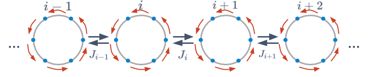
Figure 1: Pictorial representation of a clock model (with $n=6$) in a one-dimensional chain. Each site, labeled by the index $i$, has a $n$-dimensional local Hilbert space, the blue points on the circle indicate the possible states of the clocks. The red arrows represent the action of the $\tau$ operators, and hence the action of the kicks, as discussed in the main text. In the case shown here, the clocks interact through a nearest-neighbour coupling of amplitude $J_{i}$. The coupling between the sites is indicated by the double black arrow.

The model Hamiltonian $\hat{H}$ -

The evolution between two kicks is governed by the $n$-state clock Hamiltonian $\hat{H}_{n}$ Baxter89 ; Fendley2012 , see Fig.1, whose most general form is

$$\hat{H}_{n} = \sum_{i\neq j}J_{ij}\sum_{m=1}^{n-1}\alpha_{m}(\hat{\sigma}_{i}^{\dagger}\hat{\sigma}_{j})^{m}$$ (13)

$$+ \sum_{i}h_{z,i}\sum_{m=1}^{n-1}\gamma_{m}\,\hat{\sigma}_{i}^{m}+\sum_{i}h_{x,i}\sum_{m=1}^{n-1}\beta_{m}\,\hat{\tau}_{i}^{m}$$

with real couplings $J_{ij},h_{x,i},h_{z,i}$ and complex $\alpha_{m},\beta_{m},\gamma_{m}$ Note3 . The site-label $i$ runs from 1 to $L$. In the case of short-range interaction we will further assume periodic boundary condition. In order for the Hamiltonian to be Hermitian, $\alpha_{m}^{*}=\alpha_{n-m}$, $\beta_{m}^{*}=\beta_{n-m}$ and $\gamma_{m}^{*}=\gamma_{n-m}$. While $J_{ij}$ accounts for the interaction between different sites, $h_{x,i}$ ($h_{z,i}$) represent a transverse (longitudinal) field. In the absence of longitudinal field ($h_{z,i}=0$, $\forall i$) the Hamiltonian has a $\mathbb{Z}_{n}$ symmetry generated by

$$\hat{X}=\prod_{i=1}^{L}\hat{\tau}_{i}\;.$$

Together with the analysis for generic $n$, in the rest of the paper we will consider several different choices of the couplings, encompassing both a disordered short-range model as well as an infinite-range case. In these specific cases we will perform explicit numerical/analytical calculations. For future reference these specific cases are summarised Table 1.

		$n=3$	$n=4$
Short-Range interaction (SR)	$J_{ij}=J_{i}\delta_{i+1,j}$	$\alpha_{1}=\alpha_{2}^{*}=e^{i\varphi}$	$\alpha_{2}=1$, $\alpha_{1}=\alpha_{3}^{*}=(1-\eta)e^{i\varphi}/2$
		$\beta_{1}=\beta_{2}^{*}=e^{i\varphi_{x}}$	$\beta_{2}=\eta$, $\beta_{1}=\beta_{3}^{*}=\delta$
		$\gamma_{1}=\gamma_{2}^{*}=e^{i\varphi_{z}}$	$\gamma_{2}=1$, $\gamma_{1}=\gamma_{3}^{*}=\delta$
Long-Range interaction (LR)	$J_{ij}=-\frac{J}{L}$	$\alpha_{1}=\alpha_{2}^{*}=1/2$	$\alpha_{2}=\eta J^{\prime}/J$, $\alpha_{1}=\alpha_{3}^{*}=(1-\eta)/2$
	$h_{x,i}=-h$	$\beta_{1}=\beta_{2}^{*}=1$	$\beta_{2}=2\eta h^{\prime}/h$, $\beta_{1}=\beta_{3}^{*}=1-\eta$
		$\gamma_{1}=\gamma_{2}^{*}=0$	$\gamma_{1}=\gamma_{2}=\gamma_{3}=0$

Table 1: A summary of the various choices of couplings that we will analyse in the paper. We will consider both short- and long-range systems (SR and LR respectively). In the cases $n=3$ and $n=4$ the coefficients $\alpha_{m},\beta_{m},\gamma_{m}$ will parameterised as specified in the table. For $n=4$, $J,J^{\prime},h,h^{\prime}\geq 0$ and the parameter $0\leq\eta\leq 1$ will control the transition between time-crystals with different symmetries.

More specifically the first model we will discuss is a short-range disordered $n$-state clock model. Both the nearest-neighbour coupling $J_{i}$ and $h_{x,i}$/ $h_{z,i}$ will be real random numbers uniformly distributed in the intervals $[J_{z}/2,3J_{z}/2]$ and $[0,h_{z}]$ respectively. Only the strength of the interactions and of the fields are allowed to vary over the chain, $\alpha_{m}$, $\beta_{m}$ and $\gamma_{m}$ are site-independent. For the long-range case we will consider a generalisation of the Lipkin-Meshkov-Glick Lipkin model. The Hamiltonian has a $\mathbb{Z}_{n}$ symmetry generated by $\hat{X}$, as well as an invariance under sub-systems permutations. Despite its simplicity the model Hamiltonian contains, as we will show, the necessary ingredients to realise a time-crystal, in particular an extensive number of symmetry breaking eigenstates. For $n=4$, the parameters of the Hamiltonian can be adjusted to favour a phase either with $\mathbb{Z}_{4}$ spontaneously symmetry breaking states, or a phase with lower $\mathbb{Z}_{2}$ symmetry breaking states.

Time evolution during a kick -

The kicks are local, acting on each site independently, i.e. $\hat{K}=\sum_{i}\tilde{K}_{i}$. It is convenient to discuss the evolution due to the kicks by introducing the operator $\hat{X}^{(n)}_{\epsilon}$ as

$$e^{-i\hat{K}^{(n)}_{\epsilon}}\equiv\left[\hat{X}^{(n)}_{\epsilon}\right]^{p}.$$ (14)

(the superscript $n$ and the subscript $\epsilon$ are made explicit as they are essential in characterising the type of kick). Indeed the generic kick will depend on the parameter $\epsilon$ that will be varied in order to probe the stability of the time-crystal phase.

In the ideal case, the kicking is $p$-times the application of the operator $\hat{X}^{(n)}_{\epsilon=0}=\prod_{i=1}^{L}\hat{\tau}_{i}$. Assuming for simplicity $p=1$, if the operator $\hat{\tau}_{i}$ acts over an eigenstate of $\hat{\sigma}_{i}$ its effect is simply to exchange it with another eigenstate [see Eq. (11)]. The state returns back to itself after the action of $n$ times $\hat{\tau}$. A measure of the expectation of $\hat{\sigma}_{i}$ witnesses naturally the period $n$-tupling.

It is convenient to write the perfect-swapping kicking operator $\hat{X}^{(n)}_{\epsilon=0}$ as

$$\hat{X}^{(n)}_{\epsilon=0}\equiv\hat{X}=\prod_{i=1}^{L}\hat{\tau}_{i}=\prod_{i=1}^{L}\textrm{e}^{i(\pi/n)\hat{\Theta}_{i}^{(n)}}$$ (15)

where $\hat{\Theta}^{(n)}_{i}$ is an Hermitian matrix acting in the $i$-th site. Specifically, for the cases $n=2,3$ or $4$, $\hat{\Theta}$ has the form

$$\hat{\Theta}^{(2)} = \left(\begin{array}[]{cc}-1&1\\ 1&-1\end{array}\right),$$ (18)

$$\hat{\Theta}^{(3)} = \frac{2}{\sqrt{3}}\left(\begin{array}[]{ccc}0&i&-i\\ -i&0&i\\ i&-i&0\end{array}\right),$$ (22)

$$\hat{\Theta}^{(4)} = \left(\begin{array}[]{cccc}3&-1-i&-1&-1+i\\ 1-i&3&-1-i&-1\\ -1&-1+i&3&-1-i\\ -1-i&-1&-1+i&3\end{array}\right)\,.$$ (27)

Using the previous parameterisation, the perturbed kicking operator is defined as

$$\hat{X}^{(n)}_{\epsilon}=\prod_{i=1}^{L}\textrm{e}^{{i\left(\frac{\pi}{n}+\epsilon\right)\hat{\Theta}^{(n)}_{i}}}.$$ (28)

In the next Sections we will discuss in details the phase diagram for the different versions of the clock Hamiltonian. We first discuss the case of short-range interactions, the infinite-range interacting limit will be analysed in Sec. V.

IV Disordered short-range model

In this Section we are going to focus on the short-range disordered version of the Hamiltonian Eq. (13) (see also Table 1) and we denote it as $\hat{H}_{n}^{(SR)}$. Disorder is essential for the time-crystal physics in this context. It leads to many-body localisation thus preventing heating up to infinite temperature. In this regime all the eigenstates in the spectrum of $\hat{H}_{n}^{(SR)}$ posses a long-range glassy order in the thermodynamic limit Pollmann14 . The absence of heating, starting from a state with long-range order and driving, guarantees that such order persists in the dynamics. On passing, we also note that, to our knowledge, this is the first time the many-body localised state has been analysed in a clock model.

Following in spirit the same approach used for the spin-1/2 case Else2016a we first consider a set of couplings in Eq. (9) so that the Floquet eigenstates can be computed exactly. This is going to form the basis for the classification of possible time-crystal phases for generic $n$. We then move to the analysis of the robustness of such a phase under perturbations in the evolution. In this case, as already mentioned, the presence of many-body localisation is the key to stabilise the time-crystal. We will conclude this Section with a more detailed discussion of the specific cases $n=3$ and $n=4$.

IV.1 Classification of time-crystals: $h^{x}=0$

Let us start by considering the simplest possible situation: zero transverse field ($h_{x,i}=0$, $\forall i$) and an ideal-swapping kick operator as defined in Eq. (15). In this case, the operator $\hat{\sigma}_{i}$ commutes with $\hat{H}_{n}^{(SR)}$. It evolves after one period $T$ according to the Floquet operator $\hat{U}(T)$ as

$${\hat{U}}(T)^{\dagger}\hat{\sigma}_{i}{\hat{U}}(T)=\omega^{p}\hat{\sigma}_{i}$$ (29)

and then goes back to itself after a time $qT$, where $q$ is the smallest positive integer such that $qp$ is a multiple of $n$. Before discussing whether these oscillations at subharmonic frequency are the manifestation of a period $q$ time-crystal, it is useful to analyse the properties of Floquet states and quasi-energies. In this case they can be written out explicitly and – as we are going to show – they obey the properties stated in Section II for time-translation symmetry breaking to occur.

It is convenient to distinguish two cases: (i) the integers $p$ and $n$ are coprime, and (ii) the integers $p$ and $n$ have $\mbox{gcd}(p,n)=s>1$.

• The integers $p$ and $n$ are coprime - In this case it is not hard to see that $q=n$. As we discuss in Appendix A, we note that $\hat{U}(T)^{n}=e^{-in\hat{\bar{H}}}$ where

  $$\hat{\bar{H}}=\sum_{i}J_{i}\sum_{m=1}^{n-1}\alpha_{m}\,(\hat{\sigma}_{i}^{\dagger}\hat{\sigma}_{i+1})^{m}.$$ (30)

  The eigenstates of $\hat{\bar{H}}$ can be labeled by the sequence $\{s_{i}\}$, with $s_{i}=1,\omega,\dots,\omega^{n-1}$, such that

  $$\hat{U}^{n}\ket{\{s_{i}\}}=e^{-inT\mu^{+}(\{s_{i}\})}\ket{\{s_{i}\}}$$

  and

  $$\mu^{+}(\{s_{i}\})=\sum_{i}J_{i}\sum_{m=1}^{n-1}\alpha_{m}(s_{i}^{*}s_{i+1})^{m}\;.$$

  Given a configuration $\{s_{i}\}$, the states $\ket{\{s_{i}\}}$, $\hat{U}\ket{\{s_{i}\}}$, $\dots$, $\hat{U}(T)^{n-1}\ket{\{s_{i}\}}$ are degenerate (and inequivalent) eigenstates of $\hat{U}(T)^{n}$. They are not eigenstates of $\hat{U}(T)$. We denote as $\ket{\psi(\{s_{i}\},k)}$ (with $k=0,\dots,n-1$) the linear combinations of these states that diagonalise $\hat{U}(T)$:

  $$\hskip 22.76228pt\ket{\psi(\{s_{i}\},k)}=\frac{1}{\sqrt{n}}\sum_{m=0}^{n-1}\omega^{km}e^{-imT\mu^{+}(\{s_{i}\})}\hat{U}^{m}\ket{\{s_{i}\}}$$ (31)

  which satisfy

  $$\hskip 22.76228pt\hat{U}(T)\ket{\psi(\{s_{i}\},k)}=\omega^{k}e^{-iT\mu^{+}(\{s_{i}\})}\ket{\psi(\{s_{i}\},k)}.$$

  These eigenstates have quasi-energies $\mu^{+}(\{s_{i}\})-2\pi k/n$, forming multiplets of states with $2\pi/n$ splitting in quasi-energy.
  

• The integers $p$ and $n$ have $\mbox{gcd}(p,n)=s>1$ - In this case the period of the time-crystal is $q=n/s$. The Floquet operator satisfies $\hat{U}(T)^{q}=e^{-iq\hat{\bar{H}}}$ (see Appendix A) where now

  $$\hskip 22.76228pt\bar{H}=\sum_{i}J_{i}\sum_{m=1}^{n-1}\alpha_{m}\,(\hat{\sigma}_{i}^{\dagger}\hat{\sigma}_{i+1})^{m}+\sum_{i}h_{z,i}\sum_{m=1}^{n/q-1}\gamma_{mq}\,\hat{\sigma}_{i}^{mq}$$ (32)

  The states $\ket{\{s_{i}\}},\hat{U}(T)\ket{\{s_{i}\}},\dots,\hat{U}(T)^{q-1}\ket{\{s_{i}\}}$ are all degenerate (and inequivalent) eigenstates of $\hat{U}(T)^{m}$ but they are not eigenstates of $\hat{U}(T)$. One can construct the $q$ linear combinations (labeled by $k=0,\dots,q-1$) that diagonalise $\hat{U}(T)$:

  $$\hskip 22.76228pt\ket{\psi(\{s_{i}\},k)}=\frac{1}{\sqrt{q}}\sum_{m=0}^{q-1}\omega^{km}e^{-imT\mu^{+}(\{s_{i}\})}\hat{U}^{m}\ket{\{s_{i}\}}$$ (33)

  They satisfy

  $$\hskip 22.76228pt\hat{U}(T)\ket{\psi(\{s_{i}\},k)}=\omega^{k}e^{-iT\mu^{+}(\{s_{i}\})}\ket{\psi(\{s_{i}\},k)}$$

  forming multiplets of states with $2\pi/q$ splitting in quasi-energy.

In both cases discussed above Floquet states are cat states: the correlators of the local observable $\hat{\sigma}$ for two sites $i$ and $j$ is

$$\braket{\psi(\{s_{i}\},\omega^{k})}{\hat{\sigma}_{i}^{\dagger}\hat{\sigma}_{j}}{\psi(\{s_{i}\},\omega^{k})}=s_{i}^{*}s_{j}\neq 0,$$ (34)

while $\braket{\hat{\sigma}_{i}}=0$ for every site $i$. Correlations show a “glassy” long-range order, where $\braket{\hat{\sigma}_{i}^{\dagger}\hat{\sigma}_{j}}$ can assume the values $1,\omega,\dots,\omega^{n-1}$ depending on the sites. Therefore, $|\braket{\sigma_{i}^{\dagger}\sigma_{j}}|=1$ and correlations do not vanish in the limit $|i-j|\rightarrow\infty$. Each state $\ket{\psi(\{s_{i}\},k)}$ is a cat state consisting of a superposition of $q$ product states. The condition of the Floquet states being long-range correlated in order to have the time-translation symmetry breaking is fulfilled.

It is important to check whether the Floquet spectrum is non-degenerate. Floquet states organise in multiplets, each one separated by $2\pi/q$ from the other (see Section II).

The cat states $\ket{\psi(\{s_{i}\},k)}$ found above are eigenstates even for $J_{i}=0$, but their long-range correlations cannot be the evidence of a truly many-body effect. In this case the correlations are a consequence of an unusual choice of basis set. In the non-interacting case, the Floquet spectrum is extensively degenerate and many choices of Floquet states basis are possible. In particular, the Floquet operator can be diagonalised by tensor products of single-site states which are clearly not long-range correlated. Even if at a particular point in the parameter space the systems shows a time-crystal dynamics, any tiny perturbation (for example by slightly changing the kicking and taking the one in Eq. (28) with $\epsilon\ll 1$) will destroy sub-harmonic oscillations. The perturbation splits the degeneracy and selects a basis of Floquet states which are short-range correlated.

Interactions are needed to remove all the degeneracies and stabilise the time-crystal phase. Furthermore, the interactions must be such that there are no degeneracies in the Floquet spectrum. If there are degeneracies in the spectrum, one could in principle construct a linear combination of different Floquet states with the same quasi-energy satisfying cluster property. As we are going to show in the next section, any local perturbation can resolve this degeneracy: it selects the Floquet states obeying the cluster property, therefore spoiling the time-translation symmetry breaking.

In the presence of disordered couplings degeneracies are quite unlikely. Nevertheless, as we are going to show, they can occur and one must choose certain parameters in order to avoid those cases. As before, we must distinguish two cases.

• The integers $p$ and $n$ are coprime - In this case the quasi-energies are of the form

  $$\hskip 22.76228pt\mu(\{s_{i}\},k)=\sum_{i}J_{i}\sum_{m=1}^{n-1}\alpha_{m}(s_{i}^{*}s_{i+1})^{m}-2\pi k/n.$$ (35)

  For each set of $\{s_{i}\}$, the quantity $s_{i}^{*}s_{i+1}$ assumes one of the $n$ possible values $1,\omega,\dots,\omega^{n-1}$, corresponding to the $n$ possible angles between the two hands of the clock. If two such values yield the same energy $\sum_{m=1}^{n-1}\alpha_{m}(s_{i}^{*}s_{i+1})^{m}$, then the spectrum is degenerate. Therefore, we have degeneracies if there exist two integers $k_{1}$ and $k_{2}$ (with $0\leq k_{1}<k_{2}\leq n-1$) such that

  $$\sum_{m=1}^{n-1}\alpha_{m}\omega^{mk_{1}}=\sum_{m=1}^{n-1}\alpha_{m}\omega^{mk_{2}}$$ (36)

  On the other hand, if no integers $k_{1}$ and $k_{2}$ satisfy this condition, the spectrum is not degenerate and a time crystal is possible. The same condition has been found in the context of parafermionic chains as a criterion for the existence of strong edge zero modes Fendley2012 . Furthermore, in Ref. Jermyn2014 the same condition for strong edge modes is discussed, especially for the case $n=3$, for which it coincides with the presence of chiral interactions (see section IV.3).

• The integers $p$ and $n$ have $\mbox{gcd}(p,n)=n/q>1$ - In this case the quasi-energies are of the form

  $$\mu(\{s_{i}\},k) = \sum_{i}J_{i}\sum_{m=1}^{n-1}\alpha_{m}(s_{i}^{*}s_{i+1})^{m}$$ (37)

  $$+ \sum_{i}h_{z,i}\sum_{m=1}^{n/q-1}\gamma_{mq}\,s_{i}^{mq}-2\pi k/q\,.$$

  With respect to the previous case, the condition that

  $$\sum_{m=1}^{n-1}\alpha_{m}\omega^{mk_{1}}\neq\sum_{m=1}^{n-1}\alpha_{m}\omega^{mk_{2}}$$ (38)

  for every pair of integers $0\leq k_{1}<k_{2}\leq n-1$ is sufficient but not necessary to have a time crystal. If, for any pair of integers $k_{1}$ and $k_{2}$ violating Eq.(38), and for every $s_{i}=1,\dots,\omega^{n-1}$ the inequality

  $$\sum_{m=1}^{n/q-1}\gamma_{mq}(s_{i})^{mq}\neq\sum_{m=1}^{n/q-1}\gamma_{mq}\,s_{i}^{mq}\,\omega^{mq(k_{2}-k_{1})}$$ (39)

  is satisfied, then no degeneracies occur. Note that if $k_{2}-k_{1}$ is a multiple of $n/q$, then Eq.(39) is an equality for every $s_{i}=1,\dots,\omega^{n-1}$ and the spectrum is still degenerate. Since the couplings and the local fields are taken from a random continuous distribution, no degeneracies occur in the spectrum due to additional symmetries as e.g. translation invariance. Other degeneracies would require infinitely fine-tuned couplings.

IV.2 Robustness: $h_{x}\neq 0$, $\epsilon\neq 0$

In the case on which a transverse field is present, $h_{x}\neq 0$, and/or for a general form of the kick (see Eq. (28)) it is not possible to solve the model exactly. It is still possible to study the system for small perturbations from the solvable case.

Let $\hat{U}_{\lambda}(T)$ be the perturbed Floquet operator ($\hat{U}_{0}(T)$ is the unperturbed case) where $\lambda$ generically parameterises the strength of the perturbation in the kicking and/or in $\hat{H}$. Following Hastings2010 , the time crystal described above is robust for sufficiently small $\lambda$ if there is a non-zero local spectral gap. A naive explanation of what local spectral gap means can be given using simple perturbation theory. Since the perturbation is local, it can have non-zero matrix elements only between pairs of states that differ locally. On the other hand, if two states differ globally they can only be connected at an order $O(L)$ in perturbation theory, where $L$ is the size of the system, so they do not mix at any perturbative order in the limit $L\rightarrow\infty$. We define the local spectral gap as the gap between states which are connected at a finite order in perturbation theory, not scaling with $L$. This is an important point because, in the thermodynamic limit, the relevant parameter in the perturbative expansion is not the ratio between $\lambda$ and the typical gap (which becomes exponentially small) but the ratio between $\lambda$ and the local spectral gap. If this ratio is sufficiently small, a unitary operator connecting unperturbed eigenstates with perturbed ones can be constructed order by order in perturbation theory. Moreover, assuming that the Hamiltonian satisfies a Lieb-Robinson bound Liebello , it is possible to prove that the resulting transformation is local Hastings2010 ; Else2016a ; De_roeck_2015 . For translationally invariant models, one does not expect to find local spectral gaps, and this unitary transformation is in general non local. In the presence of disorder, on the other hand, the system can exhibit many-body localisation and local gaps can exist.

The presence of a non-zero local gap guarantees the existence of a region of the parameter space where the eigenstates of the system are connected to the unperturbed ones by a local unitary $\hat{V}_{\lambda}$:

$$\hat{V}_{\lambda}\ket{\psi_{0}(\{s_{i}\},k)}=\ket{\psi_{\lambda}(\{s_{i}\},k)}$$ (40)

where $\hat{V}_{\lambda}$ depends continuously on $\lambda$. The argument applies to a generic small perturbation of $\hat{U}(T)$, irrespective of its specific form Keyserlingk2016 . As shown in Appendix B, in our model the existence of the local mapping $\hat{V}_{\lambda}$ and its continuity with respect to $\lambda$ have the following relevant consequences:

1. the dressed operators $\tilde{\sigma}_{i,\lambda}=\hat{V}_{\lambda}^{\dagger}\hat{\sigma}_{i}\hat{V}_{\lambda}$ are local operators exhibiting long range correlations on the eigenstates $\ket{\psi_{\lambda}(\{s_{i}\},k)}$:

   $$\braket{{\psi_{\lambda}}(\{s_{i}\},k)}{\tilde{\sigma}_{i,\lambda}^{\dagger}\tilde{\sigma}_{j,\lambda}}{{\psi_{\lambda}}(\{s_{i}\},k)}=s_{i}^{*}s_{j}.$$ (41)

   Hence, the perturbed system fulfills the definition of time crystal.

2. up to corrections that are exponentially small in the system size, the order parameter operator $\tilde{\sigma}_{i,\lambda}$ evolves by acquiring a phase $\omega$ at each period

   $$\hat{U}(T)^{\dagger}\tilde{\sigma}_{i,\lambda}\hat{U}(T)=\omega^{p}\tilde{\sigma}_{i,\lambda}+O(e^{-cL}).$$ (42)

   After a time $mT$, corrections are of the order $mO(e^{-cL})$, meaning that for sufficiently large $m$ they destroy the oscillations. Therefore, the time scale at which we expect oscillations to decay grows exponentially with $L$. Due to locality, the undressed operator $\hat{\sigma}_{i}$ has some finite overlap with $\tilde{\sigma}_{i,\lambda}$: it will also show persistent oscillations (just, with a smaller amplitude).

3. the spectrum is made of multiplets of states with exact $2\pi/q$ splitting in the thermodynamic limit. For finite size systems, this is only valid up to corrections of the order $O(e^{-cL})$.

The arguments given above apply to generic $n$, and are in agreement with what has been found numerically for the specific case of period doubling $n=2$ [see Ref. Else2016a, ].

If the unperturbed spectrum has no local gap, the argument proving the stability of the oscillations does not apply: states that differ only locally can have the same quasi-energy. A local perturbation mixes these states and splits the degeneracy, such that the new eigenstates correspond to physical states with no long range correlations. If the spectrum is (locally) degenerate, the oscillations in Eq. 29 can become unstable to some arbitrarily small perturbations, meaning that no time crystal can be observed in an experiment. This point further clarifies the need for the absence of degeneracies in the Floquet spectrum and is in agreement with the fact that many-body localisation induced by disorder is needed in order to have a non-zero local gap everywhere in the spectrum Huse2013 . In the next subsections we are going to corroborate the findings presented so far with a numerical analysis for the cases with $n=3$ and $n=4$.

IV.3 Phase diagram - $n=3$

In this case the parameters $\alpha_{m}$, $\beta_{m}$, $\gamma_{m}$ can be expressed in terms of three angles $\varphi$, $\varphi_{x}$, $\varphi_{z}$ as indicated in the central column of Table 1. The parameter $\varphi$ defines the chirality of the model; when $\varphi=0\ (\mathrm{mod}\ \pi/3)$, the model is non-chiral or Potts model otherwise it is termed chiral-clock model Zhuang2015 ; Samajdar2018 .

It is useful to recap how the general analysis of Section IV.1 applies to this specific model when the solvable point ($h_{x}=0$, $\epsilon=0$) is considered. The Floquet states appear in triplets given by Eq. (31) with $n=3$ whose quasi-energies are respectively $\mu^{+}(\{s_{i}\})$, $\mu^{+}(\{s_{i}\})-2\pi/3$ and $\mu^{+}(\{s_{i}\})+2\pi/3$ with $\mu^{+}(\{s_{i}\})=\sum_{i}J_{i}(e^{i\varphi}s_{i}^{*}s_{i+1}+{\rm H.\,c.})$ [see Eq. (35)]. For each pair, $s_{i}^{*}s_{i+1}$ can assume three possible values $1,\omega,\omega^{2}$ and the corresponding interaction energies of the pair are $2J_{i}\operatorname{\Re{\rm e}}(e^{i\varphi})$, $2J_{i}\operatorname{\Re{\rm e}}(\omega e^{i\varphi})$ and $2J_{i}\operatorname{\Re{\rm e}}(\omega^{2}e^{i\varphi})$. Because of the disorder in $J_{i}$ (which makes other degeneracies unlikely), a degeneracy in the Floquet spectrum is possible only if the model is non-chiral and $\varphi=0\ (\mathrm{mod}\ \pi/3)$ [Fig. (2)].

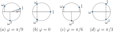
Figure 2: The dots on the circle indicate the possible values of $e^{i\varphi}s_{i}^{*}s_{i+1}$. In the non chiral case (for example $\varphi=0$ and $\varphi=\pi/3$) different values of $e^{i\varphi}s_{i}^{*}s_{i+1}$ have the same real part: the spectrum is degenerate. In the chiral case (for example $\varphi=\pi/9$ and $\varphi=\pi/6$) there is no degeneracy.

We numerically simulate the dynamics of this model with the kicks defined in Eq. (28) using exact diagonalisation of finite-size systems and then we extrapolate to the thermodynamic limit utilizing finite size scaling. We do that by probing the order parameter $\mathcal{Z}_{3}^{[\hat{\sigma}]}(t)$ defined in Eq. (5) (we remind that $t$ is discrete and is a multiple of the driving period $T$). In the solvable case ($h_{x}=0$, $\epsilon=0$) it is easy to use the analysis of Sec. IV.1 and see that $\mathcal{Z}_{3}^{[\hat{\sigma}]}(t)=1$ for every $t$ and therefore period 3 oscillations last forever. The data shown in the following are typically averaged over 100 disorder configurations, the variance is small on the scale of the figures. We start considering the effect of a transverse field $h_{x}$ for different values of the chirality parameter $\varphi$.

For a sufficiently small $h_{x}$, $\mathcal{Z}_{3}^{[\hat{\sigma}]}(t)$ reaches a plateau after a small time, with $\operatorname{\Re{\rm e}}{\mathcal{Z}_{3}^{[\hat{\sigma}]}}<1$ and $\operatorname{\Im{\rm m}}{\mathcal{Z}_{3}^{[\hat{\sigma}]}}\sim 0$ (see of Fig. (3)-(a)). Oscillations with respect to the value of the plateau are observed for a single configuration of disorder. They tend to disappear when we take the disorder-averaged values Note3 . The order parameter $\operatorname{\Re{\rm e}}{\mathcal{Z}_{3}^{[\hat{\sigma}]}(t)}$ decays from the constant value of the plateau to $0$ after a time $t^{*}$ which increases with the system size. For increasing values of $h_{x}$, the time-crystal behavior is destroyed and the plateau disappears: we can see an instance of that in Fig. (3)-(b).

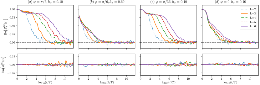
Figure 3: Time evolution of the order parameter $\mathcal{Z}_{3}^{[\hat{\sigma}]}(t)$ for $n=3$ with distinct transverse fields $h_{x}$ and distinct chiralities $\varphi$. We notice the absence of time crystal in the non-chiral case $\varphi=0$. Numerical parameters: $\epsilon=0$, $T=1$, $J_{z}=1$, $h_{z}=0.9$, $\varphi_{z}=0$, $\varphi_{x}=0$ and the results are averaged over 100 disorder realizations. Error bars (not shown in the plots) are of the order $10^{-2}$.

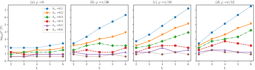
Figure 4: Dependence of $t^{*}$ as defined in the text on the size of the system for different values of $h_{x}$ and $\varphi$. In the chiral case $t^{*}$ grows exponentially for sufficiently small $h_{x}$, and becomes independent on the size for large $h_{x}$. As we get closer to the non-chiral case, the dependence gets flatter and flatter until at $\varphi=0$ we do not see the exponential growth for any value of $h_{x}$.

In Fig. 3-(c) and Fig. 3-(d) we consider the effect of the chirality parameter $\varphi$. We show the time dependence of $\mathcal{Z}_{3}^{[\hat{\sigma}]}(t)$ for different values of $\varphi$. When $\varphi$ is close to the non-chiral case oscillations are less stable. We compare the case $\varphi=\pi/36$ [Fig. 3-(c)] and $\varphi=\pi/6$ [Fig. 3-(a)] for the same value of $h_{x}$: we see that the exponential increase of $t^{*}$ with the size $L$ is slower. As predicted, when $\varphi=0$ and the solvable Hamiltonian is degenerate, no time-crystal was observed, even for small values of $h_{x}$, [see Fig. 3-(d)]. Here we have a numerical confirmation of the role of degeneracies is in making time-translation symmetry oscillations extremely fragile to perturbations.

A more accurate analysis, where we estimate $t^{*}$ as the time at which $\operatorname{\Re{\rm e}}{\mathcal{Z}_{3}^{[\hat{\sigma}]}(t)}$ reaches 0.5, indicates that $t^{*}$ exponentially increases with the system size when $\varphi\neq 0$ (see panels (b), (c) and (d) of Fig. 4). In the thermodynamic limit $t^{*}\to\infty$ and the period-tripling oscillations are persistent: the system is a time crystal as we predicted in Section IV.2. As we can see in panel (a) of Fig. 4, no exponential growth is found in the non-chiral case: $t^{*}$ is essentially independent on the size of the system, thus no time crystal in the thermodynamic limit. Based on these results, we can infer that the critical value of $h_{x}$ that represents the transition to a normal phase gets smaller and tends to 0 as $\varphi$ approaches the non-chiral value $\varphi=0$. We will confirm this picture by studying the spectral-triplet properties and mapping a full phase diagram in $h_{x}$-$\varphi$ plane.

As we discussed in Section II, the presence of triplets in the spectrum with $2\pi/3$ quasi-energy splitting is necessary in order to have a period-tripling behavior. We expect to see finite-size corrections to the splitting of the order $O(e^{-cL})$, as we have discussed in Sec. IV.2. In order to probe spectral triplets we study the quantities

$$\Delta^{\alpha}_{0}=\mu_{\alpha+1}-\mu_{\alpha}$$ (43)

$$\Delta^{\alpha}=|\mu_{\alpha+\mathcal{N}}-\mu_{\alpha}-2\pi/3|$$ (44)

where the quasi-energies $\mu_{\alpha}$ are sorted from the lowest to the greatest value in the first Floquet Brillouin zone $[0,2\pi/T]$ and $\mathcal{N}=3^{L-1}$. Since the total number of states is $3^{L}$, the quasi-energies $\mu_{\alpha+\mathcal{N}}$ and $\mu_{\alpha}$ are separated by one third of the levels of the spectrum. If the system is a time crystal, for a finite (but large) $L$ we expect to find values of $\Delta^{\alpha}$ much smaller than the level spacing between two subsequent quasi-energies $\Delta_{0}^{\alpha}\sim 2\pi/3^{L}$.

In Fig. 5 we plot the dependence of $\log_{10}\Delta^{\alpha}-\log_{10}\Delta_{0}^{\alpha}$ as a function of $1/L$. The quantity is averaged over all the Floquet quasi-energies $1\leq\alpha\leq 3\mathcal{N}$ and over different disorder configurations. When the parameters $\varphi$ and $h_{x}$ are chosen such that the system is a time crystal, we expect to find by extrapolation that $\overline{\log_{10}\Delta^{\alpha}}-\overline{\log_{10}\Delta_{0}^{\alpha}}\rightarrow-\infty$ in the thermodynamic limit. On the contrary, for a generic spectrum with Poisson statistics (but no $2\pi/3$ triplets) this quantity should diverge with increasing $L$.

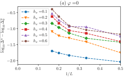
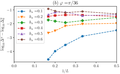
Figure 5: Scaling of the spectral ratio $\overline{\log_{10}\Delta^{\alpha}-\log_{10}\Delta_{0}^{\alpha}}$ with the system size, for different values of the chirality parameter $\varphi$.

Fig. 5-(a) refers to the non-chiral model. The plot shows that, for every value of $h_{x}$ in the range selected, $\overline{\log_{10}\Delta^{\alpha}-\log_{10}\Delta_{0}^{\alpha}}$ does not converge to $0$ as we increase the system size. On the contrary, this quantity increases with $L$. This confirms the absence of a time-crystal for the non-chiral clock model.

For the chiral clock model with $\varphi=\pi/36$, the results shown in Fig. 5-(b) are consistent with the presence of a time crystal phase for $h_{x}$ sufficiently small ($h_{x}\simeq 0.1\div 0.2$). A transition from the time crystal phase to a normal phase is suggested for larger values of $h_{x}$: $\overline{\log_{10}\Delta^{\alpha}-\log_{10}\Delta_{0}^{\alpha}}$ is expected to increase as $1/L$ goes to $0$ for $h_{x}\gtrsim 0.3$, and decrease for $h_{x}\lesssim 0.1$. However, the small size of the systems that can be analysed is a serious constraint to the possibility to make precise predictions.

In order to systematically analyse the dependence of the spectral gaps on the strength of the perturbation $h_{x}$, we study the quantities $\overline{\log_{10}\Delta^{\alpha}}$ and $\overline{\log_{10}\Delta_{0}^{\alpha}}$ as functions of $\log_{10}h_{x}$.

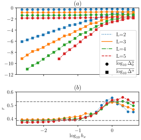
Figure 6: (a) Averaged value of the logarithms of the spectral gaps $\overline{\log_{10}\Delta_{0}^{\alpha}}$, $\overline{\log_{10}\Delta^{\alpha}}$ as a function of $\log_{10}h_{x}$. (b) quasi-energy level statistic ratio $r$ as a function of $\log_{10}h_{x}$. Dashed lines represent the value for Poisson statistics (0.386) and for Wigner-Dyson (0.527). Data were obtained for the chiral case $\varphi=\pi/18$.

In Fig. 6-(a) we consider a chiral case ($\varphi=\pi/18$). We first notice that $\overline{\log_{10}\Delta_{0}}$ does not depend on $h_{x}$, consistently with the fact that $\Delta_{0}\sim 2\pi/3^{L}$ for every value of $h_{x}$. On the opposite, $\overline{\log_{10}\Delta}$ linearly increases with $\log h_{x}$ with an angular coefficient linear in $L$ up to a critical value $h_{c}$ (a clearer evidence of this fact will be given in Fig. 8). These results are consistent with a dependence of the form $\Delta\propto(h_{x})^{L}$ for $h_{x}$ much smaller than a critical value $h_{c}$. For large $h_{x}$ the triplets disappear and $\Delta$ will tend to a constant value.

The transition is also revealed by the quasi-energy average spectral ratio defined as

$$r=\overline{\left(\frac{\min(\delta_{\alpha},\delta_{\alpha+1})}{\max(\delta_{\alpha},\delta_{\alpha+1})}\right)}$$ (45)

with $\mu_{\alpha}$ in increasing order and $\delta_{\alpha}=\mu_{\alpha+1}-\mu_{\alpha}$. The average is performed over the whole spectrum and over disorder. This quantity is a useful signature of the level statistics and can be used to discriminate ergodic from many-body localised phases  Oganesyan2006 ; D_Alessio_2014 ; Ponte2014 . For small $h_{x}$, $r$ is close to the value of $0.386$ expected for a Poisson statistics (Fig. 6-(b)). This is an evidence for many-body localization, because it shows the absence of level repulsion. When $h_{x}$ approaches the critical value, significant deviations from the Poisson limit can be observed, signaling a transition in the level statistics. Therefore the melting of the time crystal is accompanied by a transition of the dynamics towards an ergodic behaviour.

The non-chiral model, where there is no time-crystal, has substantially different spectral properties from the chiral model.

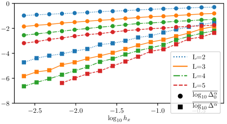
Figure 7: Averaged value of the logarithms of the spectral gaps $\overline{\log_{10}\Delta_{0}^{\alpha}}$, $\overline{\log_{10}\Delta^{\alpha}}$ as a function of $\log_{10}h_{x}$. Data were obtained for the non-chiral case $\varphi=0$.

In Fig. 7 we show the dependence of $\overline{\log_{10}\Delta_{0}^{\alpha}}$ and $\overline{\log_{10}\Delta^{\alpha}}$ on $\log h_{x}$. A comparison with Fig. 6 highlights some significant differences. The gaps $\log\Delta^{\alpha}$ have a weaker dependence on $L$ than in the chiral case and the quantity $\overline{\log_{10}\Delta_{0}^{\alpha}}$ is not constant with respect to $\log h_{x}$. The dependence of the gap $\Delta_{0}$ between two consecutive levels on $h_{x}$ is due to the fact that some eigenstates are degenerate in the absence of the perturbation: when $h_{x}\neq 0$ a gap that depends on the perturbation strength is opened between them.

A rough estimate of the critical value of $h_{x}$ can be obtained in the chiral case from the scaling $\Delta/\Delta_{0}\propto(h_{x}/h_{c})^{L}$. From an analysis of the plots, we can assume that this relation is valid when $h_{x}$ is much smaller than $h_{c}$. The data in the linear region (for small $h_{x}$) of Fig. 6 are fitted with the expression

$$\overline{\log\Delta}-\overline{\log\Delta_{0}}=\log c+L\log h_{x}-L\log h_{c}$$

with $\log c$ and $\log h_{c}$ as fitting parameters. In the inset of Fig. 8 the dashed lines represent the linear relation derived from the fit. From the fitting parameter $\log h_{c}$ (the grey vertical line in Fig. 8) we obtain $h_{c}\simeq 0.48$. In Fig. 8 we show the collapse of the curves in the inset when we rescale the quantities with the system size: this confirms the validity of the scaling we assumed for $\Delta/\Delta_{0}$.

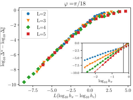
Figure 8: Averaged values of $\overline{\log_{10}\Delta^{\alpha}}-\overline{\log_{10}\Delta_{0}^{\alpha}}$ as a function of $L(\log_{10}h_{x}-\log_{10}h_{c})$, for different system sizes and $\varphi=\pi/18$. In the inset, the same quantity is plotted versus $\log_{10}h_{x}$: dashed lines are the result of the fitting procedure in the region of small $h_{x}$. The vertical grey line corresponds to the critical value $h_{c}$.

In order to further prove that the time-crystal phase disappears in the non-chiral model, it is possible to use the same fitting procedure to extrapolate an estimate of the critical value $h_{c}$ for different values of $\varphi$. We expect that stability is lost in the proximity of the non-chiral case, so $h_{c}\rightarrow 0$ as $\varphi$ approaches the value $\varphi=0$.

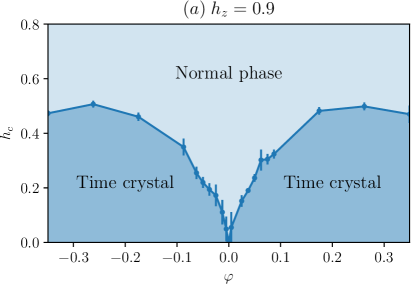
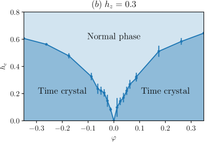
Figure 9: The curve represents the critical value $h_{c}$ as a function of the chirality parameter $\varphi$. It corresponds to the transition from the time crystal phase to a normal phase.

An estimate of the critical value $h_{c}$ is derived as we vary $\varphi$ and it is shown in Fig. (9) for two different values of $h_{z}$. The curve that we get with this procedure represents the transition from the time crystal phase to a normal phase. Both plots confirm that the time crystal is less and less stable as $\varphi$ tends to 0.

In the non-chiral case we also checked the stability of the time crystal to perturbations in the kicking (the case $\epsilon\neq 0$ in Eq. (28)) and there is no transverse field. Similarly to the case $h_{x}\neq 0$, numerical simulations show that oscillations of the order parameter decay after a time that grows exponentially in the system size if the perturbation amplitude $\epsilon$ is sufficiently small (Fig. 10). For larger values of $\epsilon$ oscillations decay much faster until time crystal behaviour is lost.

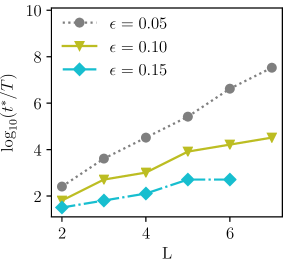
Figure 10: Dependence of $t^{*}$ (time before period-tripling oscillations decay) on the system size for distinct kicking perturbations $\epsilon$. We consider here the chiral case $\varphi=\pi/6$.

IV.4 Phase diagram - $n=4$

The $n=4$ case is the minimal model where it is possible to investigate transitions between time-crystals of different periodicity. To this end we need to consider also terms with $m=2$ in Eq.(13) (see the corresponding entry in the Table 1). The Hamiltonian $\hat{H}$ is composed of different competing terms: a term favouring states breaking spontaneously a $\mathbb{Z}_{4}$ symmetry, and another term favouring states breaking a lower $\mathbb{Z}_{2}$ symmetry, we write here explicitly for convenience the case $\delta=0$ (see Table 1):

$$\hat{H}_{4,\eta}^{(SR)} =\sum_{i}J_{i}\left[\hat{\sigma}_{i}^{2}\hat{\sigma}_{i+1}^{2}+\frac{(1-\eta)}{2}(e^{i\varphi}\hat{\sigma}_{i}^{\dagger}\hat{\sigma}_{i+1}+{\rm H.\,c.})\right]$$

$$+\sum_{i}h_{z,i}\hat{\sigma}_{i}^{2}+\eta\sum_{i}h_{x,i}\hat{\tau}_{i}^{2}.$$ (46)

where $\eta$ parameterises the competing symmetry broken phases. The Floquet operator is of the type $\hat{U}_{\eta}(T)=e^{-iT\hat{H}_{\eta}^{(SR)}}\hat{X}$, with $n=4$ clock variables and kick operator $\hat{X}$ as given by Eq. (15).

In the limit $\eta=0$, the Hamiltonian in Eq.(IV.4) is of the type discussed in Section IV.1 and is expected to support a time crystal with period $4$. On the other hand, for $\eta=1$ the operators $\hat{\sigma}_{i}^{2}$ and $\hat{\tau}_{i}^{2}$ commute among themselves and with $\hat{H}_{\eta}^{(SR)}$. Given the common eigenstates of these operators $\ket{\{s_{i},t_{i}\}}$, they satisfy $\hat{\sigma}_{i}^{2}\ket{\{s_{i},t_{i}\}}=s_{i}\ket{\{s_{i},t_{i}\}}$, $\hat{\tau}_{i}^{2}\ket{\{s_{i},t_{i}\}}=t_{i}\ket{\{s_{i},t_{i}\}}$. These states are eigenstates of ${\hat{U}_{\eta=1}(T)}^{2}$ with eigenvalue Note5 $\left(\prod_{i}t_{i}\right)\exp\left[-2iTE(\{s_{i},t_{i}\})\right]$ where we have defined $E(\{s_{i},t_{i}\})=\sum_{i}J_{i}s_{i}s_{i+1}+\sum_{i}h_{x,i}t_{i}$. The Floquet states are

$$\ket{\psi(\{s_{i},t_{i}\},\pm)}=$$

$$=\frac{1}{\sqrt{2}}\left(1\pm\left(\prod_{i}t_{i}\right)^{1/2}\textrm{e}^{iT\,E(\{s_{i},t_{i}\})}\hat{U}_{\eta=1}\right)\ket{\{s_{i},t_{i}\}}$$ (47)

and the corresponding quasi-energies $E(\{s_{i},t_{i}\})+\frac{\pi}{2}\left(\prod_{i}t_{i}\right)\mp\frac{\pi}{2}$. Floquet states are indeed long-range correlated and there is $\pi$-spectral pairing. Moreover, due to disorder and the presence of the $\hat{\tau}^{2}$ term, the spectrum is not degenerate. Therefore we expect to have a time crystal with period doubling.

Let us consider now the behaviour of the system for intermediate values of $\eta$. The Hamiltonian $\hat{H}_{\eta}^{(SR)}$ has the property that $\hat{U}_{\eta}^{\dagger}\hat{\sigma}^{2}_{j}\hat{U}_{\eta}=-\hat{\sigma}^{2}_{j}$ for every value of $\eta$. This suggests to take $\mathcal{Z}_{2}^{[\sigma^{2}]}(t)$ [see Eq. (5)] as the appropriate measure to study the robustness of the period-doubling oscillations since $\hat{U}_{\eta}^{\dagger}\hat{\sigma}_{j}\hat{U}_{\eta}=i\hat{\sigma}_{j}$ only holds for $\eta=0$.

In order to study a generic situation, we include a small perturbation $\hat{V}$ in the Floquet operator $e^{-i(\hat{H}_{\eta}+\delta\hat{V})}\hat{X}$ and study numerically the robustness of oscillations for different values of $\eta$. We considered as perturbation $\hat{V}=\sum_{i}h_{z,i}(\hat{\sigma}_{i}+\hat{\sigma}_{i}^{\dagger})+\sum_{i}h_{x,i}(\hat{\tau}_{i}+\hat{\tau}_{i}^{\dagger})$. The reason for this choice is due to $[\hat{\sigma}^{2}_{j},\hat{V}]\neq 0$, so that the perturbation will affect the dynamics of $\hat{\sigma}^{2}_{j}$ in a non-trivial way.

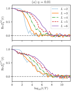
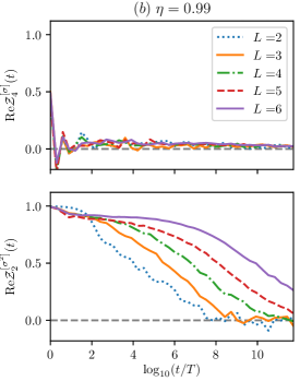
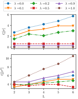
Figure 11: (a), (b) Time evolution of the order parameters $\mathcal{Z}_{4}^{[\sigma]}(t)$ (period $4$ time crystal) and $\mathcal{Z}_{2}^{[\sigma^{2}]}(t)$ (period doubling time crystal), for varying $\eta$ parameters. (c) The upper (lower) plot shows the time of the decay of period 4 (period 2) oscillations. Results are obtained with the following choice of parameters: $J_{i}$ from the uniform distribution $[1/2,3/2]$, $h_{z,i}$ from $[0,1]$, $h_{x,i}$ from $[0,1]$, $\varphi=\pi/3$, $\delta=0.1$

We show some of the results in Fig. 11. Additional data are discussed in Appendix C [Fig. 25]. As expected, $\hat{\sigma}_{j}$ has oscillations (with period $4$) only in a region close to $\eta=0$, while for $\hat{\sigma}_{j}^{2}$ we find stable oscillations (with period $2$) both close to $\eta=0$ and $\eta=1$. A period 4-tupling time crystal is found in a finite region of parameter space around $\eta=0$ [Fig. 11-(a)], while a period doubling time crystal is found close to $\eta=1$ [Fig. 11-(b)]. Our numerical analysis does not allow to draw reliable conclusions at intermediate values of $\eta$, because of the small system sizes. Although the model could in principle support a direct transition between period-doubling and period 4-tupling, it seems that in the short-range case, defined by Eq.(IV.4), the two phases appear to be probably separated by an intermediate normal region. In the next Section we will show that the situation is dramatically different in the long-range case where a direct transition between the two time-crystal phases is indeed found.

V Infinite-range model

We now turn to the analysis of the Floquet dynamics with the infinite-range version of the Hamiltonian in Eq. (13) and denote it as $\hat{H}_{n}^{(LR)}$. Here, the physical origin of the time crystal with period $qT$ lies in the existence of a phase of $\hat{H}_{n}^{(LR)}$ where a $\mathbb{Z}_{n}$ symmetry of the Hamiltonian is broken to a lower symmetry $\mathbb{Z}_{n/q}$ (if $n/q>1$ is an integer) or fully broken (if $q=n$) by an extensive amount of energy eigenstates. On initialising the system in one of the symmetry breaking manifolds, the state is brought cyclically between those manifolds even if the kick is not perfectly swapping. Consequently the order parameter of the symmetry breaking cycles among $q$ values. This mechanism was behind the time crystal with $q=n=2$ considered in Ref. Russomanno2017 and applies also to the more general cases we discuss here.

The analysis of the infinite-range case will proceed as follows. In Section V.1 we discuss how to use the permutation symmetry of the Hamiltonian to restrict to the even symmetry sector and – in that sector – map the Hamiltonian to a $n$-site bosonic model. The $\mathbb{Z}_{n}$ symmetry is mapped to a discrete translation symmetry of the boson model. Details of this mapping will be presented in Appendix D. A detailed analysis of spontaneous symmetry breaking occurring in $\hat{H}_{n}^{(LR)}$ is reported in Appendix E. Here we focus on the time-crystal behaviour. In Section V.2 we analyse specifically the cases with $n=3$ and $4$. As in the previous cases the time crystal is detected by analysing the peak in the Fourier spectrum of the order parameter at the characteristic q-tupling frequency (see Eq. (6) and the related discussion). Because we restrict to the even symmetry sector, we can study quite large system sizes and perform a finite-size scaling of the height of the peak and of its position showing that there is a time crystal in cases where the interaction Hamiltonian shows symmetry breaking. In the same section we report on a direct transition between different time-crystal phases, by varying the $\eta$ parameter in the Hamiltonian (see Table 1). More specifically, we study the transition from a period-doubling to a period 4-tupling time crystal. In Section V.3 we study the dynamics of the local observables of these models in the semiclassical limit. In this way, we can study the existence of the period $n$-tupling directly in the thermodynamic limit.

V.1 Mapping to a bosonic Hamiltonian and the semiclassical limit

Due to the infinite-range nature of the interactions in the model Hamiltonian, and the form of the kicking term, the Floquet operator has a symmetry generated by the invariance under permutation of its subsystems. We focus our analysis on the symmetric subspace, here the Hamiltonian can be represented in terms of boson operators, providing in this way a description of the system which is simpler and more manageable for numerical implementation. The main idea is to associate to each position of the clock-variable a bosonic mode. More precisely, given a set of bosonic operators $\{\hat{b}_{j}\}$, satisfying the usual commutation relations,

$$\left[\hat{b}_{\ell},\hat{b}^{\dagger}_{\ell^{\prime}}\right]=\delta_{\ell,\ell^{\prime}},\quad\left[\hat{b}_{\ell},\hat{b}_{\ell^{\prime}}\right]=0,$$ (48)

for $\ell=1,...,n$, the Hamiltonian operators are described in this bosonic representation as follows (see Appendix D for details)

$$\sum_{i=1}^{L}\hat{\sigma}_{i} = \sum_{\ell=1}^{n}\hat{n}_{\ell}\omega^{\ell-1}\;\;\;\;\;\;\;\;\sum_{i=1}^{L}\hat{\sigma}_{i}^{2}=\sum_{\ell=1}^{n}\hat{n}_{\ell}\omega^{2(\ell-1)}$$ (49)

$$\sum_{i=1}^{L}\hat{\tau}_{i} = \sum_{\ell=1}^{n}\hat{b}_{\ell}\hat{b}^{\dagger}_{\ell+1}\;\;\;\;\;\;\;\;\;\;\sum_{j=1}^{L}\hat{\tau}_{j}^{2}=\sum_{\ell=1}^{n}\hat{b}_{\ell}\hat{b}^{\dagger}_{\ell+2}$$ (50)

where $\hat{n}_{\ell}=\hat{b}_{\ell}^{\dagger}\hat{b}_{\ell}$. In the bosonic variables the Hamiltonian in Eq. (13) is represented as a closed chain of $n$ bosonic sites, with fixed number of $L$ bosonic particles. Its explicit expression is

$$\hat{H}_{n}^{(LR)}=-\frac{J}{L}\sum_{\ell,\ell^{\prime}=1}^{n}\sum_{m=1}^{n-1}\alpha_{m}\omega^{m(\ell-\ell^{\prime})}\hat{n}_{\ell}\hat{n}_{\ell^{\prime}}+$$

$$-h\sum_{\ell=1}^{n}\sum_{m=1}^{n-1}\beta_{m}\hat{b}_{\ell}\hat{b}^{\dagger}_{\ell+m}$$ (51)

(see also Table 1).

It is important to emphasise that the $\mathbb{Z}_{n}$ symmetry breaking in the clock representation is mapped to the breaking of the invariance under translation of the sites in the bosonic representation. As an illustrative example, the states breaking the rotational symmetry $\hat{X}$ with fully aligned clock operators $|s\rangle^{\otimes L}$, for $s=\omega^{\ell}$, are represented in the bosonic language by states in which all $L$ bosons occupy a single site $\ell$ (“$|0_{1}...L_{\ell}...0_{n}\rangle$” in number representation). From now on we will consider only the bosonic representation of this Hamiltonian.

In this representation the kicking operator corresponds to a global translation in the sites of the chain. Indicating with $b^{\prime}$ the bosonic operators after the kick, the unperturbed kicking, Eq. (15), reads

$$\left(\begin{array}[]{c}\hat{b}_{1}^{\prime}\\ \hat{b}_{2}^{\prime}\\ \vdots\\ \hat{b}_{n}^{\prime}\end{array}\right)=\hat{\tau}\left(\begin{array}[]{c}\hat{b}_{1}\\ \hat{b}_{2}\\ \vdots\\ \hat{b}_{n}\end{array}\right),\,\vspace*{0.3cm}$$ (52)

where $\hat{\tau}$ is the $n\times n$ matrix defined in Eq. (12). In other words, the kicking corresponds to a global translation by a single site ($\ell\rightarrow\ell+1$) in the bosonic chain. In the general case, the kicking acquires a more intricate form,

$$\left(\begin{array}[]{c}\hat{b}_{1}^{\prime}\\ \hat{b}_{2}^{\prime}\\ \vdots\\ \hat{b}_{n}^{\prime}\end{array}\right)=\exp\left[{i\left(\frac{\pi}{n}+\epsilon\right)\hat{\Theta}^{(n)}}\right]\left(\begin{array}[]{c}\hat{b}_{1}\\ \hat{b}_{2}\\ \vdots\\ \hat{b}_{n}\end{array}\right)\,.$$ (53)

where $\hat{\Theta}^{(n)}$ is the $n\times n$ matrix defined in Eq. (18).

The limit of $L\to\infty$ is equivalent to the limit where the bosonic modes are macroscopically occupied and the dynamics is described by a semiclassical equation like the Gross-Pitaevski one. In this limit we can show that the dynamics of the bosonic model is governed by a classical effective Hamiltonian, generalising the analysis done for the Bose-Hubbard dimer reported in smerza . To this aim we use the transformation $\hat{b}_{\ell}=\sqrt{L\,\hat{p}_{\,\ell}/n}\,\textrm{e}^{i\hat{\phi}_{\ell}}$ where, in order to preserve the bosonic commutation relations, we have to assume $[\hat{\phi}_{\ell},\,\hat{p}_{\,\ell^{\prime}}]=in\delta_{\ell\,\ell^{\prime}}/L$. In the limit $L\to\infty$ the commutators are vanishing and the dynamics is classical. It is induced by the effective Hamiltonian Note7 ${\cal H}_{n}^{(LR)}$

$${\cal H}_{n}^{(LR)}=-\frac{J}{n}\sum_{\ell,\ell^{\prime}=1}^{n}\sum_{m=1}^{n-1}\alpha_{m}\omega^{m(\ell-\ell^{\prime})}p_{\ell}p_{\ell^{\prime}}+$$

$$-h\sum_{\ell=1}^{n}\sum_{m=1}^{n-1}\beta_{m}\sqrt{p_{\ell}p_{\ell+m}}e^{i(\phi_{\ell}-\phi_{\ell+m})}$$ (54)

where the Poisson brackets between the canonical coordinates and momenta are $\{\phi_{\ell},\,p_{\,\ell^{\prime}}\}=\delta_{\ell\,\ell^{\prime}}$, $\{\phi_{\ell},\,\phi_{\ell^{\prime}}\}=0$, $\{p_{\,\ell},\,p_{\,\ell^{\prime}}\}=0$ . The Hamiltonian (V.1) conserves the total number of bosons to the value $L$, this reflects in the classical Hamiltonian conserving the sum of the momenta to the value 1. This fact allows to restrict the dynamics to $n-1$ pairs of canonical coordinates and momenta.

The kicking operator is described in the bosonic language by Eq. (53). Using the relation $\hat{b}_{\ell}=\sqrt{L\hat{p}_{\,\ell}/n}\,\textrm{e}^{i\hat{\phi}_{\ell}}$ this peaceful linear transformation becomes a strongly non-linear object when expressed in terms of the variables $p_{\,\ell}$ and $\phi_{\ell}$. In conclusion we can study if the model shows time-translation symmetry breaking in the thermodynamic limit looking at the classical dynamics of an Hamiltonian system with $n-1$ degrees of freedom; we are going to perform this analysis first in the case $n=3$ and $n=4$ with $\eta=0$ in the next subsection and then in the case $n=4$ with $\eta\neq 0$, studying a transition between distinct time-crystal phases.

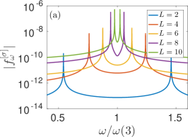
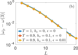
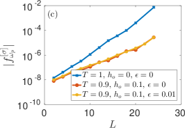
Figure 12: Time-crystal behavior for a system with $n=3$. (Numerical parameters: $J=1$, $h=0.5$ and $N_{T}=2^{15}$). (a) Fourier transform of the order parameter $\left\langle\hat{\sigma}\right\rangle_{t}$. The initial state here is given by a symmetry-breaking ground state of the static Hamiltonian $\hat{H}_{n=3}^{(LR)}$, the period $T=1$ and there is no perturbation in the kicking operator ($\epsilon=0$). (b-c) Finite-size scaling for the position of the dominant frequencies ($\omega_{p}$) and the height of the corresponding peak ($f^{[\sigma]}_{\omega_{p}}$); different initial states and different perturbations to the dynamics are considered.

V.2 Time-crystal phases

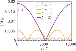
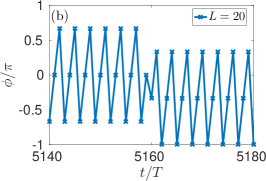
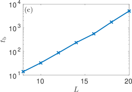
Figure 13: Time-evolution for the order parameter Eq. (55) for a system with $n=3$, $J=1$, $h=0.5$ and $T=1$. (a) Time-evolution for the absolute value $|\left\langle\hat{\sigma}\right\rangle_{t}|$ for different system sizes. (b) Time-evolution for the phase $\phi(t)$ across the Rabi oscillation period $t_{b}$. (c) Scaling of the Rabi-oscillation period $t_{b}$ with the system size.

We first focus on the analysis of the cases $n=3$ and $n=4$ with $\eta=0$, and study the existence of a discrete time crystal fully breaking the $\mathbb{Z}_{n}$ symmetry. Later on we will consider the case $n=4$ with $\eta\neq 0$ which can show a transition between distinct time crystal orders. We consider the Floquet operator Eq. (9) with $p=1$ and infinite-range interactions, expressed in the bosonic representation. In the rest of this Section we will study the dynamics of the sets of operators $\hat{\sigma}=L^{-1}\sum_{i}\hat{\sigma}_{i}$, and $\hat{\sigma}^{2}=L^{-1}\sum_{i}\hat{\sigma}_{i}^{2}$. The expectation values of $\hat{\sigma}_{i}$, $\hat{\sigma}^{2}_{i}$ are independent of the site-index $i$. They are therefore equivalent to the site-averages which have a simple expression in terms of the bosonic operators, see Eq. (49).

V.2.1 $n=3$, $n=4$ with $\eta=0$

We considering the dynamics of $\hat{\sigma}$ we expect the system to pass cyclically between different symmetry-breaking subspaces, where the expectation of this operator is markedly different. As we have explained in Section II, we consider the expectation value at stroboscopic times $\left\langle\hat{\sigma}\right\rangle_{t}$ and perform its discrete Fourier transform over $N_{T}$ periods [see Eq. (6)].

We start with a detailed numerical analysis in the case $n=3$. We first initialise the system in a symmetry-breaking ground state of the static Hamiltonian Note4 . We first consider the perfect-swapping kick given in Eq. (52). In Fig. 12-(a) we plot the power spectrum $|f_{\omega}^{[\sigma]}|$ for a finite-size case and see that, for a coupling $h/J$ smaller than the critical field value, there are two peaks that tend to $\omega(3)$ (Eq.(7)) as the system size is increased, Fig. 12-(b). The height of the corresponding peaks increases with the system size, see Fig. 12-(c). The system breaks the discrete time-translation symmetry $\mathbb{Z}$ to $3\mathbb{Z}$. The height of the peaks is related to the initial state of the evolution and its expectation value for the order parameter $\langle\hat{\sigma}\rangle_{t=0}$. For small system sizes the order parameter shows exponential corrections with $L$ due to finite-size effects, while for larger system sizes it scales polynomially to a finite value. We expect the peaks of the Fourier spectrum to behave in a similar way. The separation between the two peaks is exponentially small in the system size [Fig. 12-(b)]. This gives rise to oscillations of period exponentially long in $L$, which appear in the Fourier spectrum as a splitting in two of the period-tripling peak. This behavior can be seen in Fig. 13, where we show the time evolution of the order parameter

$$\langle\hat{\sigma}\rangle_{t}=|\left\langle\hat{\sigma}\right\rangle_{t}|e^{i\phi(t)}\,.$$ (55)

In Fig. 13-(a) we show its absolute value, where we see a periodic behavior with period $t_{b}(L)$ related to the oscillations. The phase $\phi(kT)$ of the order parameter shows period-tripling oscillations, as seen in Fig.13-(b), suffering a shift after every period $t_{b}(L)$. In Fig.13-(c) it is evident that the corresponding periods are exponentially large with the system size, and thus are effectively absent in the thermodynamic limit.

In order to verify that these period-tripling oscillations are not a fine-tuned behavior, we apply different perturbations to the dynamics, varying the period $T$, considering the perturbed kicking operator [Eq. (53) with $\epsilon\neq 0$], and considering different initial states (taken as symmetry-breaking ground states of $\hat{H}_{n=3}^{(LR)}-h_{o}\sum_{i}(\hat{\tau}_{i}+\hat{\tau}_{i}^{\dagger})$). In Figs.(12)-(b,c) we see that the time-crystal behaviour is indeed robust to such perturbations, whenever $h/J$ is smaller than the critical field. We see therefore that there is a time-crystal behaviour and is intimately connected to the symmetry breaking of the interaction Hamiltonian.

We have also studied the case $n=4$, which for $\eta=0$ shows essentially the same behaviour as in the previous case $n=3$, but with period 4-tupling. The situation changes drastically when $\eta\neq 0$, in this case at $n=4$ a new dynamics phase transition between period doubling and period 4-tupling appears. This will be the topic of the next subsection.

V.2.2 $n=4$, $\eta\neq 0$ - Transition between different time-crystal phases

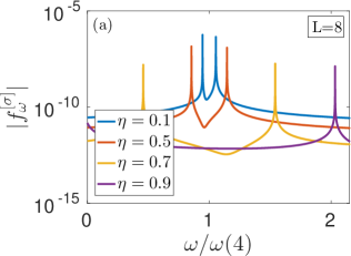
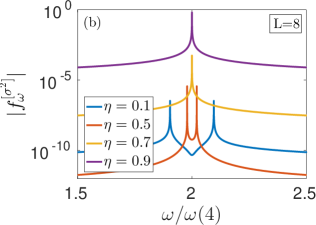
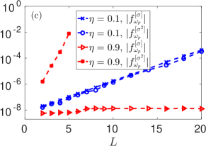
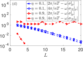
Figure 14: Distinct time-crystal phases in the model Hamiltonian $\hat{H}_{n=4,\eta}^{(LR)}$. (a,b) Fourier transforms for the order parameters $\hat{\sigma}$ and $\hat{\sigma}_{[2]}$, considering a fixed system size $L=8$. (c-d) Scaling with the system size for (c) the height of the dominant peak in the Fourier transforms and (d) its corresponding frequencies, for $\eta=0.1$ and $0.9$. (Numerical parameters: $n=4,J=J^{\prime}=1,h=h^{\prime}=0.5$ and $N_{T}=2^{15}$).

In this case the dynamics can generate distinct time-crystal phases. For $\eta$ not too large the system can break the $\mathbb{Z}_{4}$ time translation symmetry, while for larger $\eta$ it breaks a lower $\mathbb{Z}_{2}$ symmetry. We set $J=J^{\prime}=1$ and $h=h^{\prime}=1/2$, initialise the system in a symmetry-breaking ground state of $\hat{H}_{n=4,\eta}^{(LR)}$ Note6 and perform a time evolution with $2^{15}$ periods.

In Fig. 14-(a,b) we show the Fourier power spectrum for the order parameters $\left\langle\hat{\sigma}\right\rangle_{t}$ and $\left\langle\hat{\sigma}^{2}\right\rangle_{t}$ at a fixed system size $L=8$. For $\eta$ small we see two dominant peaks in $|f^{[\sigma]}_{\omega}|$ around the period 4-tupling frequency. As we increase $\eta$, the two dominant peaks of $|f^{[\sigma]}_{\omega}|$ decrease their magnitude and become farther apart from each other. On the other hand, the dominant peaks of $|f^{[\sigma^{2}]}_{\omega}|$ increase their magnitude and get closer to each other, around the period doubling frequency. This analysis for finite size suggests that there is at some point a transition from a period 4-tupling at small $\eta$ witnessed by $\hat{\sigma}$ and a period doubling at large $\eta$ witnessed by $\hat{\sigma}^{2}$.

In Fig. 14 we show the finite-size scaling analysis for the frequency of the dominant peak (Panel c) and its magnitude (Panel d) for the cases $\eta=0.1$ and $\eta=0.9$. For $\eta=0.1$ we see the behaviour of a period $4$-tupling time crystal, in which the magnitude of the dominant peak $|f^{[\sigma]}_{\omega_{\rm p}}|$ increases with the system size, with the corresponding frequency $\omega[\sigma]_{\rm p}$ approaching the period $4$-tupling frequency. The order parameter $\hat{\sigma}^{2}$ displays a period-doubling response with a similar scaling behaviour of the dominant peak $|f^{[\sigma^{2}]}_{\omega_{\rm p}}|$ and of its frequency $\omega[\sigma^{2}]_{\rm p}$. In this case, therefore, the system is a period 4-tupling time crystal.

On the opposite limit of $\eta\sim 1$ the behaviour is different. We consider the case $\eta=0.9$. Here the magnitude of the dominant peak of $f^{[\sigma]}_{\omega}$ is rather small and independent of the system size, marking the absence of a period 4-tupling time crystal phase. Furthermore, its frequency does not approach the period $4$-tupling frequency. The Fourier transform $f^{[\sigma^{2}]}_{\omega}$, however, shows the expected behaviour for a time crystal, with the dominant frequencies approaching the period doubling frequency in the thermodynamic limit and the magnitude of the corresponding peak increasing with $L$. In this case the system shows a period doubling.

The system supports distinct nontrivial time-crystal phases, breaking for $\eta\sim 0$ a discrete time-translation symmetry $\mathbb{Z}$ to $4\mathbb{Z}$, while for $\eta\sim 1$ it breaks $\mathbb{Z}$ to $2\mathbb{Z}$. The exact position of the transition between these two phases is difficult to locate using exact diagonalisation due to the limitations in the system sizes. For this goal we will use a semiclassical approach, which allows us to study the thermodynamic limit in a easier way. It is important to note that although the semiclassical approach allows us to obtain the exact behaviour in the thermodynamic limit, the finite-size scaling we have done until now was a crucial point in order to show that these symmetries are spontaneously broken only in the thermodynamic limit, as appropriate for a time crystal.

V.3 Results for the semiclassical limit

V.3.1 Case $n=3$

In this case, exploiting the conservation of $p_{1}+p_{2}+p_{3}=1$, it is convenient to apply a linear canonical transformation in the following way

$$p_{1} ={\mathcal{N}}+{m_{1}}$$ (56)

$$p_{2} ={\mathcal{N}}+{m_{2}}$$ (57)

$$p_{3} ={\mathcal{N}}-{m_{1}}-{m_{2}}\,,$$ (58)

$${\phi}_{1} =\frac{1}{3}\left(2{\theta_{2}}-{\theta_{1}}+{\Gamma}\right)$$ (59)

$${\phi}_{2} =\frac{1}{3}\left(-{\theta_{2}}+2{\theta_{1}}+{\Gamma}\right)$$ (60)

$${\phi}_{3} =\frac{1}{3}\left(-{\theta_{2}}-{\theta_{1}}+{\Gamma}\right)\,,$$ (61)

where $\{\theta_{\ell},\,m_{\ell^{\prime}}\}=\delta_{\ell\,\ell^{\prime}}$, $\{\Gamma,\,\mathcal{N}\}=1$ and all the other Poisson brackets are vanishing. It is easy to see that the Hamiltonian written in the new variables does not depend on $\Gamma$ and therefore $\mathcal{N}$ is conserved to $1/3$. The Hamiltonian in the new variables acquires the form

$${{\cal H}_{3}^{(LR)}} =-{J}\left({m_{2}}^{2}+{m_{1}}^{2}+{m_{1}}{m_{2}}\right)$$

$$-{2}h\bigg{[}\sqrt{(1+{m_{2}})(1+m_{1})}\cos({\theta_{1}}-{\theta_{2}})$$

$$+\sqrt{(1+{m_{1}})(1-m_{1}-m_{2})}\cos\theta_{1}$$

$$+\sqrt{(1-m_{1}-m_{2})(1+m_{2})}\cos\theta_{2}\,\bigg{]}\,.$$ (62)

The order parameter for the static and the time-translation symmetry breaking can be written in terms of $m_{1}(t)$ and $m_{2}(t)$ using Eq. (49) and has the form

$$\sigma=\lim_{L\to\infty}\left\langle\hat{\sigma}\right\rangle=\frac{1}{6}\left(1+3m_{2}\right)+i\frac{\sqrt{3}}{6}\left(m_{2}+2m_{1}\right)\,.$$ (63)

It is possible to find the state of minimum energy imposing $\theta_{1}=\theta_{2}=0$ and minimising the energy along the line $m_{1}=m_{2}$. There is an interval of parameters where this state has $m_{1\,{\rm eq}}=m_{2\,{\rm eq}}\neq 0$ (see Fig. 15) and therefore is triple degenerate (this can be easily seen repeating the same argument on the Hamiltonians which are obtained permuting cyclically the indices $1,2,3$ on the left side of the transformations Eqs. (56)-(61)). This fact marks the existence of a phase where there is a spontaneous breaking of the $\mathbb{Z}_{3}$ symmetry of the Hamiltonian Eq. (V.1) for $n=3$; indeed in this phase the order parameter Eq. (63) is different from zero. The critical field here is $h_{c}=0.77$ and lies within the estimate predicted using a finite-size scaling analysis (see Appendix E).

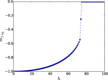
Figure 15: The value of $m_{1\,\rm eq}=m_{2\,\rm eq}$ at the minimum point of the Hamiltonian Eq. (V.3.1) versus $h$. For $h<0.77$ it is non-vanishing, marking a $\mathbb{Z}_{3}$ symmetry-breaking phase (Numerical parameters $J=1$).

After the necessary introduction to the properties of the Hamiltonian, we now focus on the kicked dynamics and the period-tripling oscillations. We apply the kicking Eq. (52) to this Hamiltonian, solve the Hamilton differential equations and see if there are period-tripling oscillations. Because $m_{1}(t)$ and $m_{2}(t)$ have a very similar behavior, we will discuss in detail the behaviour of $m_{1}(t)$ (our conclusions hold for $m_{2}(t)$ and then for the order parameter $\sigma(t)$ exactly in the same way). Let us focus on a case where the $\mathbb{Z}_{3}$ symmetry is broken in the static part of the Hamiltonian ($h=0.36J$) and let us look for the period-tripling oscillations. If present, these oscillations appear as a marked peak at the period-tripling frequency in the power spectrum of the Fourier transform of $m_{1}(t)$ [see Eq. (6)]. Remarkably we see those oscillations both in time domain (upper panel of Fig. 16) and in frequency (lower panel of Fig. 16) if we initialise the system in one of the symmetry-breaking ground states ($\theta_{1}(0)=\theta_{2}(0)=0$ and $m_{1}(0)=m_{2}(0)=m_{\rm eq}$) or if we initialise it with $\theta_{1}(0)=\theta_{2}(0)=0$ and a value of $m_{1}(0)=m_{2}(0)=m_{\rm ini}$ near to $m_{\rm eq}$. This robustness with respect to the initial state is due to the existence of an interval of energies where all the trajectories break the $\mathbb{Z}_{3}$ symmetry, as it occurs in the period doubling case (see Ref. Russomanno2017, ). We have checked this fact studying the dynamics of Hamiltonian (V.3.1) without a kicking: for the values of $m_{1}(0)=m_{2}(0)=m_{\rm ini}$ considered in Fig. 16 we can see oscillations of $m_{1}(t)$ around a non-vanishing value (see Fig. 17). This interval of energies where the trajectories break the $\mathbb{Z}_{3}$ symmetry directly corresponds to the extensive amount of eigenstates below an energy threshold which break the symmetry in the finite-size case (see Appendix E).

\begin{overpic}[width=195.12767pt]{time_crystal_31-crop}\put(-1.0,71.0){(a)}\end{overpic}

\begin{overpic}[width=195.12767pt]{trasfo_3-crop.pdf}\put(-1.0,71.0){(b)}\end{overpic}

Figure 16: (a) Evolution of $m_{1}(t)$ with the Hamiltonian (V.3.1) and the kicking (52), with $n=3$. (b) Corresponding Fourier transform [see Eq. (6)]: we see a marked peak at the period-tripling frequency $\omega(3)=2\pi/(3T)$ (Numerical parameters: $h=0.36$, $J=1.0$, $T=0.1$, $N_{T}=2048$).

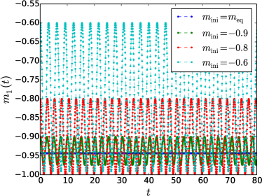
Figure 17: Evolution of $m_{1}(t)$ with the Hamiltonian (V.3.1) without any kicking, for different initial conditions. Notice the oscillations around an average value different from 0, proving the existence of an interval of energies above the minimum where the corresponding trajectories are $\mathbb{Z}_{3}$ symmetry breaking (Numerical parameters: $h=0.36$, $J=1.0$).

The dynamics is robust also against perturbations in the kicking: if we apply Eq. (53) with $n=3$ we see a full interval of $\epsilon$ where the time crystal persists. We can see this fact by studying the Fourier transform of $m_{1}(t)$: we find a marked peak at the period-tripling frequency for a full interval of $\epsilon$ around zero. The symmetry breaking oscillations of $m_{1}(t)$ in time domain are shown in the upper panels of Fig. 18. In the central panels the corresponding Fourier transforms: when $\epsilon$ is small enough there is a marked peak at the period-tripling frequency. In the lower panels it is shown how the frequency $\omega_{p}$ and the height $|f^{[m_{1}]}_{\omega_{p}}|^{2}$ of the peak in the Fourier transform depend on $\epsilon$. For all the considered initial conditions, the peak frequency deviates from $\omega(3)$ (and then the time crystal disappears) when $\epsilon>0.08$.

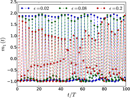
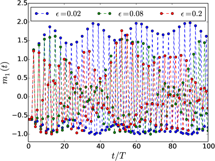
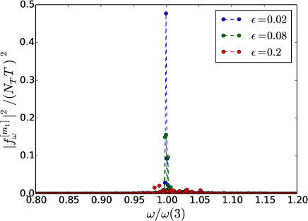
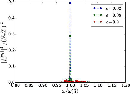
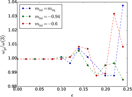
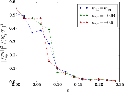
Figure 18: (Upper panels) Evolution of $m(t)$ with the Hamiltonian Eq. (V.3.1) and the $\epsilon\neq 0$-periodic kicking Eq. (52) (Numerical parameters: $h=0.36$, $J=1.0$, $T=0.1$, $m_{1}(0)=m_{2}(0)=m_{\rm eq}$ in the left panel and $m_{1}(0)=m_{2}(0)=-0.6$ in the right one). (Central panels) Corresponding Fourier transforms for $N_{T}=2048$ periods: for small $\epsilon$ we see a marked peak at the period-tripling frequency $\omega(3)=2\pi/(3T)$. (Lower panels) Position $\omega_{p}$ (left) and height $|f_{\omega_{p}}^{[m_{1}]}|^{2}$ (right) of the main peak of the Fourier power spectrum versus $\epsilon$ for different values of $m_{1}(0)=m_{2}(0)=m_{\rm ini}$. We see persistent period-tripling oscillations (main peak at $\omega_{p}=\omega(3)=2\pi/3$) for $\epsilon$ small enough ($\epsilon\leq 0.08$).

V.3.2 $n=4$, $\eta=0$

The approach is analogous to the case $n=3$. Using that $p_{1}+p_{2}+p_{3}+p_{4}=1$ we can write the effective Hamiltonian in the form

$${\cal H}_{4,\eta=0}^{(LR)} =-\frac{J}{4}\left[(m_{1}-m_{3})^{2}+(2m_{2}+m_{1}+m_{3})^{2}\right]$$

$$-2h\sqrt{(1+m_{1})(1+m_{2})}\cos(\theta_{1}-\theta_{2})$$

$$-2h\sqrt{(1+m_{2})(1+m_{3})}\cos(\theta_{2}-\theta_{3})$$

$$-2h\sqrt{(1+m_{3})(1-m_{1}-m_{2}-m_{3})}\cos(\theta_{3})$$

$$-2h\sqrt{(1-m_{1}-m_{2}-m_{3})(1+m_{1})}\cos(\theta_{1})\,,$$ (64)

where $\theta_{j}$ are canonical coordinates, $m_{j}$ are canonical momenta and obey the standard canonical commutation relations. Using Eq. (49) we can write the order parameter $\sigma$ in terms of $m_{j}$ in the form

$$\sigma=\frac{1}{4}\left[(m_{1}-m_{3})+i(2m_{2}+m_{1}+m_{3})\right]\,.$$ (65)

We can find the minimum of the Hamiltonian Eq. (V.3.2) fixing $\theta_{j}=0$ and then using a steepest descent algorithm. For $h<1$ there is a $\mathbb{Z}_{4}$ broken symmetry phase where the $m_{j\,{\rm eq}}$ and the $\sigma_{\rm eq}$ are non vanishing (see Fig. 19). There is a full interval of energies where the trajectories break the $\mathbb{Z}_{4}$ symmetry; we can see this fact in Fig. 20 where we simulate the dynamics of ${\cal H}_{4,\eta=0}^{(LR)}$ without any kicking. We choose initial conditions different from the equilibrium ones and we observe that $m_{1}(t)$ oscillates around a non-vanishing average. These are the perfect conditions for the manifestation of a period $4$-tupling time crystal. Indeed, if we apply to this system the kicking Eq. (53) with $n=4$, we see period 4-tupling oscillations which are stable if we consider initial conditions different from the lowest energy ones, $m_{2}(0)=m_{2\,{\rm eq}}$, $m_{1}(0)=m_{3}(0)=m_{1\,{\rm eq}}+\delta m$ (see Fig. 21; here we show only $m_{1}(t)$ for clarity, the situation is the same for all the $m_{j}(t)$ and for $\sigma(t)$).

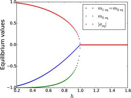
Figure 19: The values of $m_{j\,{\rm eq}}$ and $|\sigma_{\rm eq}|$ at the minimum point of the Hamiltonian Eq. (V.3.2) versus $h$. For $h<1$ they are non-vanishing, marking a $\mathbb{Z}_{4}$ symmetry-breaking phase (Numerical parameters: $J=1$).

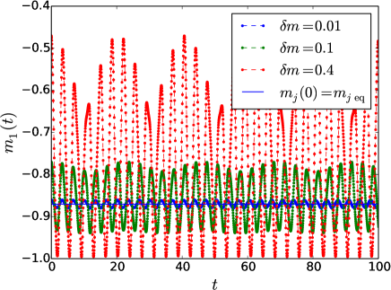
Figure 20: Evolution of $m_{1}(t)$ with the Hamiltonian Eq. (V.3.2) and no kicking. Initial conditions $\theta_{1}(0)=\theta_{2}(0)=\theta_{3}(0)=0$, $m_{2}(0)=m_{2\,{\rm eq}}$, $m_{1}(0)=m_{3}(0)=m_{1\,{\rm eq}}+\delta m$. $J=1$, $h=0.36$.

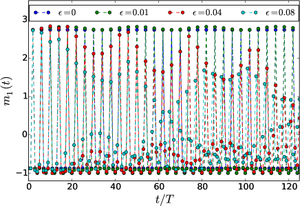
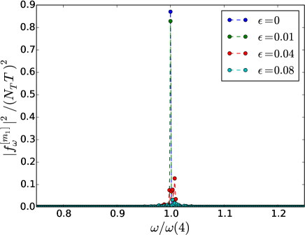
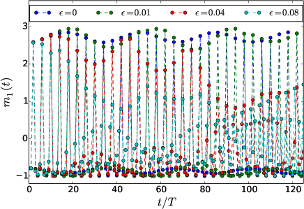
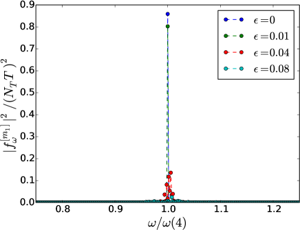
Figure 21: Dynamics of $m_{1}(t)$ with the Hamiltonian Eq. (V.3.2) and a perturbed kicking [Eq. (53)]. Time domain (left panels) and frequency domain (right panels). For $\epsilon=0.01$ we see the period 4-tupling oscillations (appearing as a peak at $\omega(4)=\pi/(2T)$ which disappear for larger $\epsilon$. Initial conditions: $\theta_{1}(0)=\theta_{2}(0)=\theta_{3}(0)=0$, $m_{2}(0)=m_{2\,{\rm eq}}$, $m_{1}(0)=m_{3}(0)=m_{1\,{\rm eq}}+\delta m$; we consider two different initial conditions, $\delta m=0$ in the upper panels and $\delta m=0.08$ in the lower ones. Numerical parameters: $J=1$, $h=0.36$, $T=0.1$.

V.3.3 $n=4$, $\eta\neq 0$ - Transition between two different time-crystal phases

We finally analyse the behaviour as a function of $\eta$. The order parameter $\sigma$ for the breaking of the $\mathbb{Z}_{4}$ symmetry is the one in Eq. (65), while the $\mathbb{Z}_{2}$-order parameter is expressed by the quantity

$$\sigma_{[2]}\equiv\lim_{L\to\infty}\left\langle\hat{\sigma}^{2}\right\rangle=(1/2)(m_{1}+m_{3})\,$$ (66)

(see Eq. (49)). The effective Hamiltonian has the form

$${\cal H}_{4,\eta}^{(LR)} =(1-\eta){\cal H}_{4,0}^{(LR)}+\eta\left[-{J^{\prime}}(m_{1}+m_{3})^{2}\right.$$

$$-2{h^{\prime}}\sqrt{(1+m_{1})(1+m_{3})}\cos(\theta_{1}-\theta_{3})$$

$$\left.-2{h^{\prime}}\sqrt{(1+m_{2})(1-m_{1}-m_{2}-m_{3})}\cos\theta_{2}\right]$$ (67)

where ${\cal H}_{4,0}^{(LR)}$ is the effective Hamiltonian shown in Eq.(V.3.2).

As previously, we start from considering the properties of the minimum-energy point of the static part of this model (we find this point through a steepest descent algorithm). The results are reported in Fig. (22): $\sigma_{[2]\,{\rm eq}}$ is always non vanishing, while $\sigma_{\rm eq}$ is nonvanishing only if $\eta$ is smaller than an $\eta_{c}$ which for this choice of parameters equals $0.8$. This means that the model breaks the $\mathbb{Z}_{4}$ symmetry for $\eta<\eta_{c}$ while it breaks only the $\mathbb{Z}_{2}$ symmetry otherwise.

The dynamics of $m_{1}(t)$ (the other $m_{j}$ behave exactly in the same way) in the presence of the kicking is shown in Fig. 23, where we consider different initial conditions, $m_{2}(0)=m_{2\,{\rm eq}}$, $m_{1}(0)=m_{3}(0)=m_{1\,{\rm eq}}+\delta m$. There are values of $\eta$ for which there is period 4-tupling (upper panel), and others for which there is period doubling (central panel). Taking a perturbed kicking with $\epsilon\neq 0$, there are value of $\eta$ where there is no time crystal (bottom panel).

By looking at the properties of the Fourier transform, we see a value $\eta_{c}$ of $\eta$ where there is a direct transition from period 4-tupling to period doubling. For $\epsilon=0$ this point coincides with the value of $\eta$ where ${\sigma}_{\rm eq}$ at equilibrium disappears (see Fig. 22). For $\epsilon\neq 0$ another value $\eta_{c\,1}>\eta_{c}$ appears such that, for $\eta>\eta_{c\,1}$, there is no time crystal behaviour. Three phases appear, a period 4-tupling one, a period doubling one and a normal one.

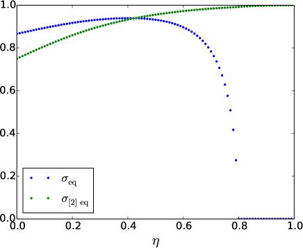
Figure 22: Order parameters versus $\eta$ in the minimum-energy state of the Hamiltonian Eq. (V.3.3) (Numerical parameters $h=h^{\prime}=0.5$, $J=J^{\prime}=1.0$).

The first transition point at $\eta_{c}$ is marked by the disappearing of the peak in the Fourier transform at the period 4-tupling frequency ($|f_{\omega_{p},\,n=4}^{[m_{1}]}|^{2}$) (see the upper left panel of Fig. 24). The peak at the period doubling frequency ($|f_{1\,\omega_{p},\,n=2}^{[m_{1}]}|^{2}$) persists until $\eta_{c\,1}$ (upper right panel of Fig. 24). The first peak, in all the period 4-tupling phase, is locked at the period 4-tupling frequency $\omega(4)$ (lower left panel of Fig. 24), while the second exists in both the time-crystal phases and is at frequency $\omega(2)$ (lower right panel of Fig. 24). (This peak is not exactly at $\omega(2)$ due the finite number of period over which we analyse the dynamics; we have checked that it tends to the correct value if we perform the Fourier transform over a number of periods $N_{T}$ larger). In the phase without time crystal, the position of the peak around the period doubling frequency slightly moves. It is not however relevant for the dynamics, since its height is vanishingly small (see upper right panel of Fig. 24). It is not surprising that in case of period 4-tupling there is a peak also at the period doubling frequency, being $\omega(2)$ one of the harmonics of $\omega(4)$. The remarkable thing is that the peak at $\omega(4)$ will disappear.

This picture is stable if we slightly perturb the kicking with $\epsilon\neq 0$ and if we take an initial state different from the symmetry breaking ground state ($\delta m\neq 0$). As we said before, when $\epsilon\neq 0$ a trivial phase appears for $\eta>\eta_{c\,1}$. We emphasise that in this analysis the initial conditions we consider depend on $\eta$, because these initial conditions correspond to the minimum-energy point for that value of $\eta$ or some point around that minimum.

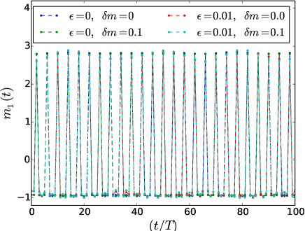
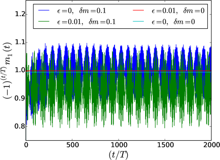
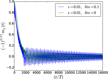
Figure 23: Evolution of $m_{1}(t)$ with the Hamiltonian Eq. (V.3.3) and the kicking Eq. (53). Both period 4-tupling for $\eta=0.36$ (upper panel) and period doubling are present for $\eta=0.82$ (central panel; the factor $(-1)^{k}$ makes the period-doubling oscillations to appear as an almost constant object). No time crystal whatsoever for $\eta=0.96$ and $\epsilon=0.01$ (lower panel). (Numerical parameters $h=h^{\prime}=0.5$, $J=J^{\prime}=1.0$).

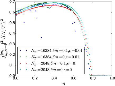
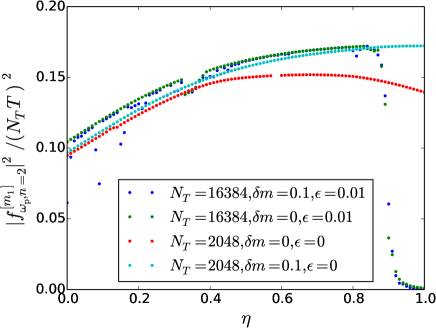
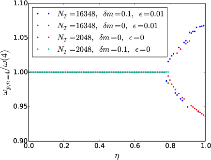
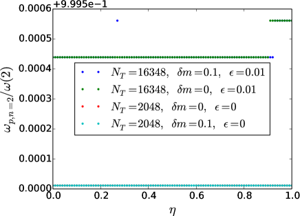
Figure 24: (Upper left panel) Peak in the Fourier transform at the period 4-tupling frequency ($|f_{\omega_{p}\,n=4}^{[m_{1}]}|$) versus $\eta$; we notice that it disappears at a value $\eta_{c}\sim 0.8$ where the period 4-tupling time-crystal phase ends up. (Upper right panel) Peak in the Fourier transform at the period doubling frequency ($|f_{\omega_{p}\,n=2}^{[m_{1}]}|$) versus $\eta$; we notice that it disappears at a value $\eta_{c\,1}>\eta_{c}$ when $\epsilon\neq 0$. For $\eta_{c}<\eta<\eta_{c\,1}$ there is a period-doubling time crystal phase, for $\eta>\eta_{c\,1}$ there is no time crystal. (Bottom left panel) In the period 4-tupling phase the peak at the period 4-tupling frequency sticks at $\omega(4)=\pi/(2T)$. (Bottom right panel) Peak at the period doubling frequency $\omega(2)=\pi/T$ (Numerical parameters: $h=h^{\prime}=0.5$, $J=J^{\prime}=1.0$).

VI Conclusions

We have studied a class of period-$n$-tupling discrete time crystals based on interacting models of $n$-clock variables. We have considered two different limits: a disordered short-range model and a clean infinite-range clock model.

In the case of disordered short-range models the stability of the time crystal is provided by many-body localisation, which prevents the system from heating up to infinite temperature and makes possible the persistence of long-range order in the dynamics. We have analysed the features of these models combining analytical results and perturbative arguments, and showed that the model supports a time crystal when there are no degeneracies in its Floquet spectrum. In this case the main characterizing properties of a time crystal are robust to perturbations, namely, (i) the presence of Floquet states with long-range correlations, (ii) Floquet quasi-energies organized in $n$-tuplets, which are shifted from each other by the period-$n$-tupling frequency, and (iii) an order parameter clock operator oscillating with the period-$n$-tupling frequency. We have found that these properties are robust up to corrections exponentially small in the system size. This implies that they become exact in the thermodynamic limit were the time-translation symmetry breaking occurs. We have corroborated our theory with a numerical analysis for the case $n=3$, which shows a period-tripling time crystal, and for $n=4$, where we constructed a model showing period $4$-tupling in one regime and period doubling in another one.

In the infinite-range case we have found that the interaction Hamiltonian has a phase where an extensive number of eigenstates breaks the $\mathbb{Z}_{n}$ symmetry in the thermodynamic limit and this was the basis for the stability of the period-$n$-tupling time crystal in such models. Due to its symmetry, generated by the invariance under permutation of its subsystems, the infinite-range model can be studied for larger system sizes, allowing us to perform a precise finite size scaling analysis. In fact, using its symmetries we have shown that the model could be mapped over a bosonic model with $n$ sites whose occupation depends on the system size. Within this picture we have numerically studied the cases $n=3$ and $4$, showing in both cases the existence of a time-translation symmetry breaking phase only in the thermodynamic limit, as appropriate for a time crystal.

In the thermodynamic limit, we have also shown that the infinite-range model is described by a classical effective Hamiltonian, where we have studied its dynamics in more detail. We have showed exactly the existence of the time crystal for $n=3$ and $n=4$. Moreover, similarly to the short-range case, we have also constructed a model whose static part could show a transition between period $n$-tupling and period $n/2$-tupling. We studied its properties in detail for the case with $n=4$. After showing the existence of the two time crystal phases by means of a finite-size scaling analysis, we used the effective classical model in the thermodynamic limit to properly study their transition. We have then verified that the model gives rise to a direct transition between the time-crystal phase with period $n$-tupling to the one with period $n/2$-tupling. To the best of our knowledge, this represents the first example in the literature of a direct transition between different time-crystal phases.

Appendix A Proof of Eqs. 30 and 32

A.1 Case 1: $p$ and $n$ are coprime

Let us define for clarity $\hat{H}=\hat{H}_{n}^{(SR)}$ By inserting a certain number of identities we can rewrite $\hat{U}^{n}$ as follows:

$$\hat{U}^{n}=e^{-iT\hat{H}}\hat{X}^{p}e^{-iT\hat{H}}\hat{X}^{-p}\hat{X}^{2p}e^{-iT\hat{H}}\hat{X}^{-2p}\hat{X}^{3p}\dots$$

$$\dots\hat{X}^{np}e^{-iT\hat{H}}\hat{X}^{-np}\hat{X}^{np}=$$

$$=e^{-iT\hat{H}}e^{-iT\hat{X}^{p}\hat{H}\hat{X}^{-p}}e^{-iT\hat{X}^{2p}\hat{H}\hat{X}^{-2p}}\dots e^{-iT\hat{X}^{np}\hat{H}\hat{X}^{-np}}$$ (68)

where we also used $\hat{X}^{np}=1$. Since all the exponentiated operators commute, we can write $\hat{U}^{n}=e^{-inT\bar{H}}$ with

$$\bar{H}=\frac{1}{n}\sum_{j=0}^{n-1}\hat{X}^{jp}\hat{H}\hat{X}^{-jp}$$

We note that $\hat{H}_{n}^{(SR)}$ contains the interaction terms, which are invariant under the transformation induced by $X^{-jp}$, and a longitudinal field containing operators $\hat{\sigma}_{i}^{m}$ (with $1<m<n-1$), which satisfy

$$\sum_{j=0}^{n-1}\hat{X}^{jp}\hat{\sigma}^{m}\hat{X}^{-jp}=\left(\sum_{j=0}^{n-1}\omega^{-jpm}\right)\hat{\sigma}^{m}.$$

If $n$ and $p$ are coprime, the sum in parentheses contains all the $n$-th roots of 1, so it vanishes. We obtain

$$\bar{H}=\sum_{i}J_{i}\sum_{m=1}^{n-1}\alpha_{m}\,(\hat{\sigma}_{i}^{\dagger}\hat{\sigma}_{i+1})^{m}.$$

A.2 Case 2: $p$ and $n$ have $gcd(p,n)=s>1$

Similarly to the previous case we can use the fact that $\hat{X}^{qp}=1$ (with $q=n/s$) to rewrite $\hat{U}^{q}$ as

$$\hat{U}^{q} =e^{-iT\hat{H}}e^{-iT\hat{X}^{p}\hat{H}\hat{X}^{-p}}e^{-iT\hat{X}^{2p}\hat{H}\hat{X}^{-2p}}\dots$$

$$\dots e^{-iTX^{qp}\hat{H}\hat{X}^{-qp}}$$ (69)

We obtain that $\hat{U}^{q}=e^{-iqT\bar{H}}$ with

$$\bar{H}=\frac{1}{q}\sum_{j=0}^{q-1}\hat{X}^{jp}\hat{H}_{n}^{(SR)}\hat{X}^{-jp}.$$

As before, the interaction terms are not affected by the action of $X^{-jp}$, but the longitudinal field is. We see that

$$\sum_{j=0}^{q-1}\hat{X}^{jp}\hat{\sigma}^{m}\hat{X}^{-jp}=\left(\sum_{j=0}^{q-1}\omega^{-jpm}\right)\hat{\sigma}^{m}.$$

The sum in parentheses is equal to $q$ when $mp=0\ (\mathrm{mod}\ n)$ (i.e. when $m$ is a multiple of $q$), it vanishes otherwise. Hence we get

$$\bar{H}=\sum_{i}J_{i}\sum_{m=1}^{n-1}\alpha_{m}\,(\hat{\sigma}_{i}^{\dagger}\hat{\sigma}_{i+1})^{m}+\sum_{i}h_{z,i}\sum_{m=1}^{n/q-1}\gamma_{mq}\,\hat{\sigma}_{i}^{mq}.$$

Appendix B Consequences of the quasi-adiabatic continuation

B.1 Long range order

In this section we will generalize some results proven in Keyserlingk2016, for the Ising model to the case of the clock model. In addition, we will use these generalized results to prove some important properties concerning time crystal order (persistence of oscillations, spectral properties), which were hinted to but not explicitly proven in Keyserlingk2016, .

The assumption that there exists a family of local unitaries $\hat{V}_{\lambda}$ (depending continuously on the perturbation strength $\lambda$), that connects perturbed and unperturbed eigenstates has many important consequences. First, as we now prove, it implies the stability of the long range order. Consider the perturbed eigenstates $\ket{{\psi}_{\lambda}(\{s_{i}\},p)}=V_{\lambda}\ket{{\psi}_{0}(\{s_{i}\},p)}$. We define the dressed operators

$$\tilde{\sigma}_{i,\lambda}=\hat{V}_{\lambda}\sigma_{i}\hat{V}^{\dagger}_{\lambda},\hskip 28.45274pt\tilde{\tau}_{i,\lambda}=\hat{V}_{\lambda}\tau_{i}\hat{V}^{\dagger}_{\lambda}$$

It follows that

$$\tilde{\sigma}^{\dagger}_{i,\lambda}\tilde{\sigma}_{i+1,\lambda}\ket{{\psi}_{\lambda}(\{s_{i}\},p)} =\hat{V}_{\lambda}\sigma^{\dagger}_{i}\sigma_{i+1}\ket{\psi_{0}(\{s_{i}\},p)}$$

$$=s_{i}^{*}s_{i+1}\ket{{\psi}_{\lambda}(\{s_{i}\},p)}$$ (70)

The unitary $\hat{V}_{\lambda}$ is equivalent to the time evolution operator of a local Hamiltonian, as a consequence of the Lieb Robinson bound the dressed operators $\tilde{\sigma}_{i,\lambda}$ are exponentially localized. Therefore, Eq. B.1 shows the existence of long range order.

B.2 Persistent oscillations

We proved that the eigenstates of $\hat{U}_{\lambda}$ are also eigenstates of $\tilde{\sigma}^{\dagger}_{i,\lambda}\tilde{\sigma}_{i+1,\lambda}$, hence

$$[\hat{U}_{\lambda},\tilde{\sigma}^{\dagger}_{i,\lambda}\tilde{\sigma}_{i+1,\lambda}]=0.$$ (71)

Using the same argument as in Keyserlingk2016, , we now prove that

$$\hat{U}_{\lambda}^{\dagger}\tilde{\sigma}_{i,\lambda}\hat{U}_{\lambda}\simeq\omega^{p}\tilde{\sigma}_{i,\lambda}$$ (72)

where Eq. (72) is valid up to a correction that is exponentially small in the system size.

Let us consider the operator $\tilde{\sigma}^{\dagger}_{i,\lambda}\tilde{\sigma}_{j,\lambda}$ with $j>i$. This can be written as a product of “l-wall” operators between neighboring sites

$$\tilde{\sigma}^{\dagger}_{i,\lambda}\tilde{\sigma}_{j,\lambda}=(\tilde{\sigma}^{\dagger}_{i,\lambda}\tilde{\sigma}_{i+1,\lambda})(\tilde{\sigma}^{\dagger}_{i+1,\lambda}\tilde{\sigma}_{i+2,\lambda})\dots(\tilde{\sigma}^{\dagger}_{j-1,\lambda}\tilde{\sigma}_{j,\lambda})$$

Since each l-wall operator commutes with $\hat{U}_{\lambda}$, we have

$$[\hat{U}_{\lambda},\tilde{\sigma}^{\dagger}_{i,\lambda}\tilde{\sigma}_{j,\lambda}]=0.$$

We can rewrite this equation as

$$\hat{U}_{\lambda}^{\dagger}\tilde{\sigma}^{\dagger}_{i,\lambda}\tilde{\sigma}_{j,\lambda}\hat{U}_{\lambda}=(\hat{U}_{\lambda}^{\dagger}\tilde{\sigma}^{\dagger}_{i,\lambda}\hat{U}_{\lambda})(\hat{U}_{\lambda}^{\dagger}\tilde{\sigma}_{j,\lambda}\hat{U}_{\lambda})=\tilde{\sigma}^{\dagger}_{i,\lambda}\tilde{\sigma}_{j,\lambda}$$ (73)

We can further manipulate this last equation by taking to the left side the operators localized in $i$ and on the right side the operators localized in $j$. We obtain

$$\tilde{\sigma}_{i}(\hat{U}_{\lambda}^{\dagger}\tilde{\sigma}^{\dagger}_{i,\lambda}\hat{U}_{\lambda})=\tilde{\sigma}_{j,\lambda}(\hat{U}_{\lambda}^{\dagger}\tilde{\sigma}_{j,\lambda}^{\dagger}\hat{U}_{\lambda})$$ (74)

We already argued that $\tilde{\sigma}_{i,\lambda}$ is exponentially localized around the site $i$. The operator $\hat{U}_{\lambda}^{\dagger}\tilde{\sigma}^{\dagger}_{i,\lambda}\hat{U}_{\lambda}$ is also localized because it can be obtained from the localized operator $\tilde{\sigma}_{i,\lambda}$ by evolving it for a time $T$ with a local time-dependent Hamiltonian. Therefore, we still expect that $\hat{U}_{\lambda}^{\dagger}\tilde{\sigma}^{\dagger}_{i,\lambda}\hat{U}_{\lambda}$ decays exponentially with the distance from the site $i$.

From Eq. (74) we deduce that the two unitary operators $\tilde{\sigma}_{i}(\hat{U}_{\lambda}^{\dagger}\tilde{\sigma}^{\dagger}_{i}\hat{U}_{\lambda})$ and $\tilde{\sigma}_{j}(\hat{U}_{\lambda}^{\dagger}\tilde{\sigma}_{j}^{\dagger}\hat{U}_{\lambda})$ are equal, even though they are localized possibly far apart on the chain. The distance between $i$ and $j$ can be of order $L$. In the thermodynamic limit, the only possibility is that these two operators are c-numbers. More precisely, they are unitary so they must be phases. If the system has a finite size $L$, the exponential localization of the two operators implies that a correction of order $O(e^{-cL})$ can be present (where $c$ is a constant that depends on the localization length of the operators). It follows that

$$\hat{U}_{\lambda}^{\dagger}\tilde{\sigma}_{i}\hat{U}_{\lambda}=e^{i\theta}\tilde{\sigma}_{i}+O(e^{-cL}).$$ (75)

Taking the $q$-th power of Eq.(75) in the thermodynamic limit we have

$$\hat{U}_{\lambda}^{\dagger}\tilde{\sigma}_{i,\lambda}^{n}\hat{U}_{\lambda}=e^{in\theta}\tilde{\sigma}_{i,\lambda}^{n}.$$

From $\tilde{\sigma}_{i,\lambda}^{n}=1$, it follows that $e^{in\theta}=1$, so $e^{i\theta}$ can only assume one of the $n$ values $1,\omega,\dots,\omega^{n-1}$.

To determine the value of $\theta$ we consider a special case: when the perturbation is absent ($\lambda=0$), $\tilde{\sigma}_{i,\lambda}$ reduces to $\sigma_{i}$ and $\hat{U}_{\lambda}$ reduces to $\hat{U}_{0}$. In this case, Eq.(75) is satisfied by $e^{i\theta}=\omega^{p}$:

$$\hat{U}_{0}^{\dagger}\sigma_{i}\hat{U}_{0}=\omega^{p}\sigma_{i}.$$

We assumed that $\hat{V}_{\lambda}$ depends continuously on the parameter $\lambda$. Hence, all the dressed quantities also depend continuously on $\lambda$. As a consequence, the phase $e^{i\theta}$ cannot change abruptly from $\omega^{p}$ to the other possible values $1$, $\omega,\dots,\omega^{n-1}$ as $\lambda$ is turned on. We must conclude that for every $\lambda$ we find $e^{i\theta}=\omega^{p}$. We get

$$\hat{U}_{\lambda}^{\dagger}\tilde{\sigma}_{i}\hat{U}_{\lambda}=\omega^{p}\tilde{\sigma}_{i}+O(e^{-cL}).$$

This implies that $\tilde{\sigma}_{i}(mT)=\hat{U}_{\lambda}^{-m}\tilde{\sigma}_{i}\hat{U}_{\lambda}^{m}=\omega^{mp}\tilde{\sigma}_{i}+mO(e^{-cL})$, meaning that oscillations persist at least up to a time that is exponentially large in $L$.

We can further argue that the undressed operator $\sigma_{i}$ has an expansion in terms of the dressed operators of the form

$$\sigma_{i}=c_{i}\tilde{\sigma}_{i,\lambda}+\dots$$

where $c_{i}\simeq O(1)$ and the other terms are exponentially localized around the position $i$. It follows that

$$\sigma_{i}(mT)\sigma_{i}^{\dagger}(0)=|c_{i}|^{2}\tilde{\sigma}_{i.\lambda}(mT)\tilde{\sigma}_{i}^{\dagger}(0)+\dots$$

As a consequence, while $\tilde{\sigma}_{i\lambda}$ oscillates with amplitude 1, the oscillations of $\sigma_{i}$ will have an amplitude $|c_{i}|^{2}<1$ for not too large times. The additional oscillations given by the other terms of the sum will average to 0 when we consider different disorder realizations. Hence we expect $\overline{\braket{\sigma_{i}}}$ to have finite amplitude oscillations, decaying to 0 after a time $t^{*}\sim O(e^{cL})$.

B.3 Spectral properties

In the exactly solvable case we showed that Floquet eigenstates are found in multiplets with $2\pi/q$ quasi-energy splitting. We are now going to show that this also happens for the perturbed system in the thermodynamic limit as long as we are in the time crystal regime.

Eq.(72) implies that $[{\hat{U}_{\lambda}}^{q},\tilde{\sigma}_{i,\lambda}]=O(e^{-cL})$, which means that the $\tilde{\sigma}_{i,\lambda}$ are approximate constants of motion in the stroboscopic evolution with period $qT$ for finite size systems. Only in the limit $L\rightarrow\infty$ they become exact constants of motion. Since all the $\tilde{\sigma}_{i,\lambda}$ commute among themselves and (approximately) commute with ${\hat{U}_{\lambda}}^{q}$, it follows that the transformed states $\hat{V}_{\lambda}\ket{\{s_{i}\}}$, being eigenstates of all the $\tilde{\sigma}_{i,\lambda}$, are (approximate) eigenstates of ${\hat{U}_{\lambda}}^{q}$. The $q$ states $\hat{V}_{\lambda}\ket{\{s_{i}\}}$, $\hat{V}_{\lambda}\ket{\{\omega^{p}s_{i}\}}$,$\dots$, $\hat{V}_{\lambda}\ket{\{\omega^{p(q-1)}s_{i}\}}$ are linear combinations of the $q$ Floquet eigenstates $\ket{{\psi}_{\lambda}(\{s_{i}\},k)}$ with $k=0,1,\dots,q-1$ defined in section IV.1. But Floquet eigenstates are, by definition, also eigenstates of ${\hat{U}_{\lambda}}^{q}$: a linear combination of them can be an eigenstate of $\hat{U}_{\lambda}^{q}$ only if they are degenerate (with respect to ${\hat{U}_{\lambda}}^{q}$). This means that, in thermodynamic limit, the $q$ Floquet eigenstates $\ket{{\psi}_{\lambda}(\{s_{i}\},k)}$ must have the same eigenvalue that we denote $\exp{(-qi\tilde{E}^{+}(\{s_{i}\}))}$.

$${\hat{U}_{\lambda}}^{q}\ket{\tilde{\psi}(\{s_{i}\},k)}=e^{-qi\tilde{E}^{+}(\{s_{i}\})}\ket{\tilde{\psi}(\{s_{i}\},k)}$$

Therefore, they can have as eigenvalues of $U_{f,\lambda}$ one of the $q$-th roots of $\exp{(-qi\tilde{E}^{+})}$: $\exp{(-i\tilde{E}^{+})}$, $\omega^{p}\exp{(-i\tilde{E}^{+})}$, $\dots$, $\omega^{p(q-1)}\exp{(-i\tilde{E}^{+})}$. Hence, the possible values of the quasi-energy gaps are $0$, $2\pi/q$, $\dots$, $2\pi(q-1)/q$. Using the continuity of the unitary $V_{\lambda}$, we can deduce that the gaps can only change continuously: since they can only assume one of the $q$ discrete values, they cannot change at all. This proves that the exact $2\pi/q$ splitting is preserved in the thermodynamic limit. For finite size systems, this fact is only valid up to corrections of the order $O(e^{-cL})$.

Appendix C Disordered $\mathbb{Z}_{4}$ clock model: from period 2 to period 4

Supplementary numerical results for section IV.4 are shown in Fig. 25.

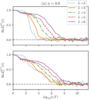
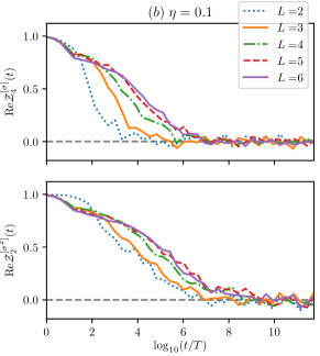
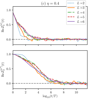
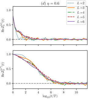
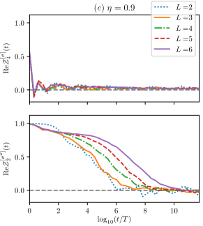
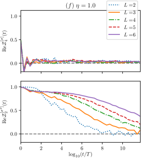
Figure 25: Time evolution of the order parameters $Z(t)$ (period $4$ time crystal) and $Z_{[2]}(t)$ (period doubling time crystal), for varying $\lambda$ parameters. Results are obtained with the following choice of parameters: $J_{i}$ from the uniform distribution $[1/2,3/2]$, $h_{z,i}$ from $[0,1]$, $g_{i}$ from $[0,1]$, $\alpha_{1}=\frac{e^{i\pi/3}}{2}$, $\epsilon=0.1$

Appendix D Mapping to a bosonic representation

We start defining the symmetrization operator $\hat{P}$ for our system with $L$ subsystems, each one composed by a clock variable of order $n$, as

$$\hat{P}=\sum_{\{\hat{\Pi}\}}\hat{\Pi}_{j_{1},...,j_{L}},$$ (76)

where $j_{i}=1,...,L$ and $\hat{\Pi}_{j_{1},...,j_{L}}$ permute the subsystems according to the $j_{i}$ indexes. As an illustrative example, $\hat{\Pi}_{1,3,2}|\sigma_{1}\sigma_{2}\sigma_{3}\rangle=|\sigma_{1}\sigma_{3}\sigma_{2}\rangle$, where $\sigma_{j}=1,\omega,...,n-1$ represents the direction of the $j$’th clock spin.

We know that symmetric subspace for a Hilbert space with $L$ subsystems can always be represented, in second quantization, in terms of bosonic operators $\{\hat{b}_{j}\}$ (Eq.(48)). We then define a basis $\{|n_{1},n_{2},...,n_{n}\rangle\}$ for this subspace as follows:

$$|n_{1}n_{2}...n_{n}\rangle \equiv \frac{1}{\sqrt{N!\prod_{k=1}^{n}n_{k}!}}\hat{P}|(1...1)_{n_{1}}(\omega...\omega)_{n_{2}}...(\omega^{*}...\,\omega^{*})_{n_{n}}\rangle$$ (77)

$$= \frac{1}{\sqrt{N!\prod_{k=1}^{n}n_{k}!}}(\hat{b}^{\dagger}_{1})^{n_{1}}(\hat{b}^{\dagger}_{2})^{n_{2}}...(\hat{b}^{\dagger}_{p})^{n_{n}}|vac\rangle$$ (78)

where the index $n_{j}$ represents the number of clock operators in the $\sigma_{j}$ direction, or alternatively, the number of bosons in the $j$’th bosonic mode, and $N=\sum_{j=1}^{n}n_{j}$ is the total number of bosons.

Since the Hamiltonian is invariant under permutation, therefore commuting with $\hat{P}$, the study of its representation in bosonic language becomes significantly simpler: we must simply analyse how it acts in a single representative clock spin configuration (right side of Eq.(77)).

The bosonic representation for the operator $\hat{\sigma}=(1/L)\sum_{j}\hat{\sigma}_{j}$ is obtained by

$$\hat{\sigma}|n_{1}n_{2}...n_{n}\rangle = \hat{P}\frac{1}{\sqrt{N!\prod_{k=1}^{n}n_{k}!}}\hat{\sigma}|(1...1)_{n_{1}}(\omega...\omega)_{n_{2}}...(\omega^{*}...\,\omega^{*})_{n_{n}}\rangle$$ (79)

$$= (1/L)(\sum_{j=1}^{n}n_{j}\omega^{j-1})|n_{1}n_{2}...n_{n}\rangle$$ (80)

where in the first line we used commutativity between $\hat{P}$ and $\hat{\sigma}$. Thus, we clearly see that

$$\hat{\sigma}=(1/L)\sum_{j}\hat{n}_{j}\omega^{j-1},$$ (81)

where $\hat{n}_{j}=\hat{b}^{\dagger}_{j}\hat{b}_{j}$. The operator $\hat{R}=\sum_{j}\hat{\tau}_{j}$ follows analogously,

$$\hat{R}|n_{1}n_{2}...n_{p}\rangle = \hat{P}\frac{1}{\sqrt{N!\prod_{k=1}^{n}n_{k}!}}\hat{R}|(1...1)_{n_{1}}(\omega...\omega)_{n_{2}}...(\omega^{*}...\omega^{*})_{n_{n}}\rangle$$ (82)

$$= \frac{\hat{P}}{\sqrt{N!\prod_{k=1}^{n}n_{k}!}}\left(n_{1}|(1...1)_{n_{1}-1}(\omega...\omega)_{n_{2}+1}...(\omega^{*}...\omega^{*})_{n_{n}}\rangle\right.$$ (84)

$$\left.+n_{2}|(1...1)_{n_{1}}(\omega...\omega)_{n_{2}-1}(\omega^{2}...\omega^{2})_{n_{3}+1}...(\omega^{*}...\omega^{*})_{n_{p}}\rangle+...\right)$$

$$= \sum_{j}\sqrt{n_{j}}\sqrt{n_{j+1}+1}|\,...\,(\omega^{j}...\,\,\omega^{j})_{(n_{j}-1)}(\omega^{j+1}...\,\,\omega^{j+1})_{(n_{j+1}+1)}\,...\,\rangle$$ (85)

Thus,

$$\hat{R}=\sum_{j}\hat{b}_{j}\hat{b}^{\dagger}_{j+1}$$ (86)

Exactly the same reasoning follows for the operators $\hat{\sigma}_{[2]}=(1/L)\sum_{j}\hat{\sigma}_{j}^{2}$ and $\hat{R}_{[2]}=\sum_{j}\hat{\tau}_{j}^{2}$. We see in this case that

$$\hat{\sigma_{[2]}} = \frac{1}{L}\sum_{j=1}^{n}\hat{n}_{j}\omega^{2(j-1)}),$$ (87)

$$\hat{R}_{[2]} = \sum_{j=1}^{n}\hat{b}_{j}\hat{b}^{\dagger}_{j+2}$$ (88)

The unperturbed kicking operator $\hat{X}_{\epsilon=0}=\prod_{j}\hat{\tau}_{j}$ acts as

$$\hat{X}_{\epsilon=0}|n_{1}n_{2}...n_{n}\rangle=|n_{p}n_{1}...n_{n-1}\rangle$$ (89)

and is thus described as a global translation of a single mode ($j\rightarrow j+1$) in the bosonic system.

Global Hamiltonian terms which are invariant under permutation, such as the kicking operator with perturbations, can also be easily described in bosonic language. Consider a general unitary operator $\hat{V}^{\rm{[sp]}}$ acting in all of the $L$ clock operators, as follows,

$$\hat{O}_{\rm{global}}=\hat{V}^{\rm{[sp]}^{\otimes L}}$$ (90)

This operator is translated to a single particle bosonic transformation in the bosonic language,

$$\hat{b}_{j}^{\prime}=\sum_{\ell}\hat{V}^{\rm{[sp]}}_{\ell,j}\hat{b}_{\ell}$$ (91)

Appendix E Spontaneous symmetry breaking in the infinite-range case

\begin{overpic}[width=140.92517pt]{gap_L_p3-crop.pdf}\put(-1.0,71.0){(a)}\end{overpic}

\begin{overpic}[width=140.92517pt]{gap_L_p4-crop.pdf}\put(-1.0,71.0){(b)}\end{overpic}

\begin{overpic}[width=140.92517pt]{Sz_ssb_p34-crop.pdf}\put(-1.0,75.0){(c)}\end{overpic}

Figure 26: (a) and (b) Scaling of the $n$-fold gap $E_{n-1}-E_{0}$ with the system size, for $\eta=0$ and $n=3$ and $4$, respectively. (c) Under a small perturbation $\hat{W}$ explicitly breaking the symmetry of the Hamiltonian, the (non-degenerated) ground state acquires a macroscopic value for the order parameter $\langle\hat{\sigma}_{i}\rangle_{\rm GS}\sim 1$ in the region where the $n$-fold gap is roughly smaller than the perturbation. System sizes: $L=50$ and $30$ for $n=3$ and $4$, respectively; $J=1$ in all the plots.

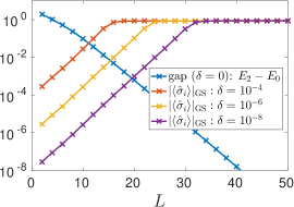
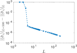
Figure 27: Finite-size effects and scaling with the size of the system for the order parameter $\langle\sigma_{i}\rangle$ in the ground state of the Hamiltonian $\hat{H}_{n}^{(\rm{LR})}+\hat{W}$, with $\hat{W}=-\delta\,\sum_{i=1}^{L}(\hat{\sigma}_{i}+\hat{\sigma}_{i}^{\dagger})$ a small perturbation breaking explicitly the symmetry of the model. We show here results for the case with $n=3$. In the left-panel we set $h/J=0.5$ and see the exponential corrections to the order parameter when $\delta\lesssim(E_{n}-E_{0})$, while in the opposed case it scales to a finite value. In the right-panel we set $h/J=0.01$ where we clearly see the polynomial scaling of the order parameter to a finite value in the thermodynamic limit.

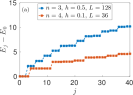
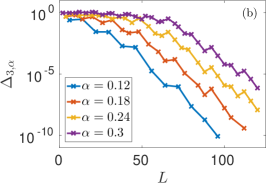
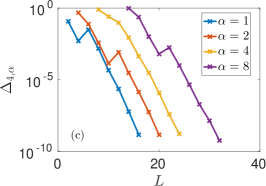
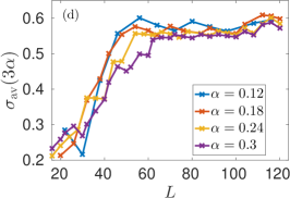
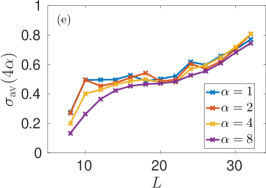
Figure 28: (a) Low-energy spectrum (shifted by the ground state energy) of the Hamiltonian $\hat{H}_{n,\eta=0}^{(LR)}$ for $n=3$ and $n=4$: the spectrum is organized in $n$-tuplets. In panels (b) and (c) we show the scaling of the $n$-tuplets energy splittings ($\Delta_{q=n,\alpha}$ as defined in Eq. (92)) with the system size. In panel (b) we show the case $n=3$ with $h=0.5$, and in (c) $n=4$ with $h=0.1$. In the panels (d) and (e) we show the scaling of the order parameter averaged over such $n$-tuplets, i.e., the averaged order parameter over the $n\alpha$ lowest eigenstates ($\sigma_{\rm av}(n\alpha)$ as defined in Eq. (93)). In panel (d) we show the case $n=3$ with $h=0.5$, and in (e) $n=4$ with $h=0.1$. $J=1$ in all the plots.

We focus here on the infinite-range version of the Hamiltonian Eq. (13) which we denote as $\hat{H}_{n,\eta}^{(LR)}$ in Sec. V. As we have remarked in Sec. V, the presence of a period $q$-tupling time-crystal phase is intimately related to the existence of an extensive amount of states that spontaneously break a $\mathbb{Z}_{q}$ symmetry and this will be the subject of this appendix. In the bosonic representation, this maps to the breaking of the translation symmetry of the model Hamiltonian.

E.0.1 Cases $n=3$ and $n=4$ with $\eta=0$

In this case, the $\mathbb{Z}_{n}$ symmetry is clearly broken when $h=0$ and, for not too large fields $h$, we should expect that this symmetry breaking persists. The symmetry breaking manifests in the thermodynamic limit as a $n$-fold degeneracy in the ground-state subspace. All the states of the system below a threshold energy, extensive in the size $L$ (broken symmetry edge $Le^{*}$), break the symmetry and the corresponding eigenenergies organize in $n$-tuplets. The order parameter characterising the symmetry breaking (in ground and excited states) is $\hat{\sigma}_{i}$.

We start considering the properties of the ground state. In Fig. (26)-(a,b,c) we analyse the properties of the ground state for $n=3$ and $4$ for finite sizes. In order to probe the existence of the $\mathbb{Z}_{n}$ symmetry breaking ground states we study the $n$-fold gap $E_{n-1}-E_{0}$ of the Hamiltonian, where $\{E_{\mu}\;(\mu=0,\,1,\,2,\ldots)\}$ are the eigenvalues of the Hamiltonian in increasing order $E_{\mu}\leq E_{\mu+1}$, with $E_{0}$ the ground state energy. In Fig. (26)-(a,b,c) we show the $n$-fold gap for different values of the system size and the coupling. For $n=3$ and $h\lesssim 0.7$ the $n$-fold gap closes exponentially fast with the system size, while for larger $h\gtrsim 0.8$ the system is $n$-fold gapped [Fig. (26)-(a)]. A similar behavior occurs for $n=4$ [Fig. (26)-(b)], where for $h<1$ the $n$-fold gap closes exponentially with the system size, while for $h=1$ the closing is polynomial $(E_{3}-E_{0})\sim L^{-1/3}$, and for larger $h>1$ the system is $n$-fold gapped.

In order to show that this $n$-fold degeneracy is actually related to a spontaneous symmetry breaking of the interaction Hamiltonian, we add a vanishingly small perturbation $\hat{W}=-\delta\,\sum_{i=1}^{L}(\hat{\sigma}_{i}+\hat{\sigma}_{i}^{\dagger})$ to the Hamiltonian Eq. (V.1) (we use $\delta=10^{-8}$), breaking explicitly its symmetry. In Fig. (26)-(c) the (non-degenerate) ground state acquires then a macroscopic value for the order parameter $\langle\hat{\sigma}_{i}\rangle_{\rm GS}\sim 1$ in the region where the $n$-fold gap is roughly smaller than the perturbation, showing the existence of the symmetry breaking. It is interesting to understand how the order parameter signaling the symmetry breaking phase depends on the perturbation $\delta$ and the size of the system. For a small perturbation $\delta\ll(E_{n}-E_{0})$, i.e., small compared to the gap of the system, we expect from first order in perturbation theory corrections which scale with the inverse of the gap. Thus, in a symmetry broken phase, these corrections due to finite-size effects should scale exponentially with the system size, see Fig. (27)-(left-panel). For larger perturbations $\delta\gtrapprox(E_{n}-E_{0})$ this picture is not valid anymore, and we find [Fig. (27)-(right-panel)] that the order parameter scales polynomially with the system size to a finite value in the thermodynamic limit.

Now we move to the excited states. In order to see if the Hamiltonian supports an extensive fraction of $\mathbb{Z}_{n}$ spontaneously symmetry breaking (SSB) states, we study if the spectrum is organised in $n$-tuplets [see Fig. 28-(a)]. In general, in order to quantify the existence of an extensive amount of $q$-tuplets, we define the quantity $\Delta_{q,\alpha}$

$$\Delta_{q,\alpha}=\sum_{\mu=1}^{\mu_{\alpha}}(E_{q\mu-1}-E_{q\mu-q})\,,$$ (92)

where $\mu_{\alpha}=\alpha L$ ($\alpha$ a finite positive number). In Figs.(28)-(b,c) we fix the coupling $h$ so that the ground states show spontaneous symmetry breaking, and we study the dependence of $\Delta_{q=n,\alpha}$ on the system size: we observe that there is an extensive fraction of the spectrum ($\alpha>0$) which is organised in $n$-tuplets, where $\Delta_{n,\alpha}$ decays exponentially fast with the system size.

In order to show that these $q$-tuply (with $q=n$) degenerate subspaces are actually related to symmetry-breaking states, we apply the vanishingly small perturbation $\hat{W}$ defined above and compute the order parameter averaged over all the states up to $\mu_{\alpha}$

$${\sigma}_{\rm av}(\alpha)=\frac{1}{\mu_{\alpha}}\sum_{\mu=1}^{\mu_{\alpha}}|\left\langle\hat{\sigma}_{i}\right\rangle_{\mu}|\,.$$ (93)

In Figs.(28)-(d,e) we notice that in the case where the extensive gap $\Delta_{q=n,\alpha}$ decays exponentially fast with system size [Figs. 28-(b,c)], the $n$-tuple eigenstates are indeed related to a SSB, showing a finite value for ${\sigma}_{\rm av}(\alpha)$. The last case corresponds to the existence of a size-independent broken-symmetry edge; we can actually see it by plotting $|\left\langle\hat{\sigma}_{i}\right\rangle_{\mu}|$ versus $E_{\mu}/L$ [Fig. 29].

\begin{overpic}[width=173.44534pt]{abs_sig_pert_p3_EjL_zoom-crop.pdf}\put(-1.0,75.0){}\end{overpic}

\begin{overpic}[width=173.44534pt]{abs_sig_pert_p4_EjL_zoom-crop.pdf}\put(-1.0,75.0){}\end{overpic}

Figure 29: $|\left\langle\hat{\sigma}_{i}\right\rangle_{\mu}|$ versus $E_{\mu}/L$ for (a) $n=3$ with $h=0.5$ and (b) $n=4$ with $h=0.1$ in a symmetry-breaking phase. $J=1$ in both cases. We see an extensive number of symmetry-breaking states below the broken-symmetry edge.

E.0.2 Different symmetry-breaking phases for $n=4$, $\eta\neq 0$

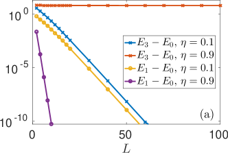
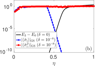
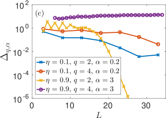
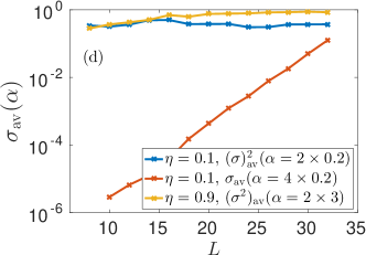
Figure 30: Different symmetry breakings in $\hat{H}_{4,\eta}^{(LR)}$. (a) Scaling of the $4$-fold gap $E_{3}-E_{0}$ and the $2$-fold gap $E_{1}-E_{0}$ with the size of the system, for parameters $\eta=0.1$ and $0.9$. (b) Under a small perturbation $\hat{W}_{[2]}$ breaking explicitly the symmetry of the Hamiltonian, the (non-degenerated) ground state acquires a macroscopic value for the order parameters $\langle\hat{\sigma}_{i}\rangle_{\rm GS}\sim 1$ or $\langle\hat{\sigma}_{i}^{2}\rangle_{\rm GS}\sim 1$, in the region where its corresponding $q$-fold gap is roughly smaller than the perturbation strength $\delta\sim 10^{-8}$. Here the system size is $L=30$ and the $2$-fold gap is negligible ($<10^{-10}$), being omitted from the figure. (c) Scaling of $\Delta_{4,\alpha}$ and $\Delta_{2,\alpha}$ [Eq. (92)] with the system size. (d) Scaling of $\sigma_{\rm av}(\alpha)$ and $(\sigma^{2})_{\rm av}(\alpha)$ (Eq. (93)) with the system size. $\sigma_{\rm av}(\alpha)$ is null in the case of $\eta=0.9$, and we thus omit it from the figure.

In this section we focus on the case $n=4$. The Hamiltonian (Eq. (V.1)) for $\eta=0$ breaks the $\mathbb{Z}_{n}$ symmetry (as we have demonstrated above), while for $\eta=1$ it breaks a lower $\mathbb{Z}_{n/2}$ symmetry (being the bosonic representation of the well-known Lipkin-Meshkov-Glick model symbreak ). The natural order parameters for these two phases are $\hat{\sigma}_{i}$ and $\hat{\sigma}_{i}^{2}$, respectively. It is interesting to understand if there is a sharp transition between these two phases at a finite value of $\eta$. In order to make this analysis, we fix $J=J^{\prime}=1$ and $h=h^{\prime}=1/2$ and study the existence of an extensive number of SSB states for different values of $\eta$. We find the persistence of the $\mathbb{Z}_{n}$ SSB phase for $\eta$ close to zero ($\eta=0.1$), and the persistence of the $\mathbb{Z}_{n/2}$ SSB phase for $\eta$ close to one ($\eta=0.9$). We find clues for a transition between the two phases at $\eta\sim 0.5$.

Let us start focusing on the case $\eta=0.1$. Concerning the ground state properties, we can see in Fig. 30-(a) that both the $4$-fold and $2$-fold gap decay to zero exponentially fast with the system size, marking the existence of a $4$-fold degeneracy in the ground state. This corresponds to a breaking of the $\mathbb{Z}_{4}$ symmetry of an extensive part of the spectrum: we can see this fact in Fig. 30-(c) where both the extensive doubling gap $\Delta_{2,\alpha}$ and the 4-tupling gap $\Delta_{4,\alpha}$ decay to zero exponentially fast with $L$. In agreement with this we find that, adding a vanishingly small perturbation $\hat{W}_{[2]}=-\delta\,\sum_{i=1}^{L}(\hat{\sigma}_{i}+\hat{\sigma}_{i}^{2}/2+{\rm H.~{}c.})$ there is an extensive amount of states with a macroscopic expectation of both $\hat{\sigma}_{i}$ and $\hat{\sigma}_{i}^{2}$. This means that both ${\sigma}_{\rm av}(\alpha)$ and $({\sigma}^{2})_{\rm av}(\alpha)$ scale to a finite value for $L\to\infty$ – the definition for $({\sigma}^{2})_{\rm av}(\alpha)$ is the same as in Eq. (93). We can see this fact in Fig. 30-(d) where for $\eta=0.1$, both ${\sigma}_{\rm av}(\alpha)$ and $({\sigma}^{2})_{\rm av}(\alpha)$ tend to a finite value when $L\to\infty$. We conclude that for $\eta=0.1$ the system breaks the $\mathbb{Z}_{4}$ and also the $\mathbb{Z}_{2}$ symmetry (which is a subgroup of $\mathbb{Z}_{4}$). Different is the case $\eta=0.9$. Here there is only the breaking of the $\mathbb{Z}_{2}$ symmetry. We can see this in the ground-state properties (only $E_{1}-E_{0}$ scales to zero when $L\to\infty$ – see Fig. 30-(a)) and in the properties of the excited states (only $\Delta_{2,\alpha}$ scales to 0 for $L\to\infty$ – panel (c) – and only $({\sigma}^{2})_{\rm av}(\alpha)$ tends to a finite value – panel (d)). The value of ${\sigma}_{\rm av}(\alpha)$ is always null in this case. There is a transition between these two phases when $\eta$ is changed and we can see this fact in Fig. 30-(b). The symmetry-breaking ground state acquires a macroscopic value for the order parameter $\langle\hat{\sigma}_{i}\rangle_{\rm GS}$ in the region $\eta\gtrsim 0.5$. Here there is $\mathbb{Z}_{4}$ symmetry breaking and the $4$-fold gap is roughly smaller than the perturbation $\hat{W}_{[2]}$. On the opposite, $\langle\hat{\sigma}^{2}\rangle_{\rm GS}\sim 1$ for all $\eta$, both for $\mathbb{Z}_{4}$ and $\mathbb{Z}_{4}$ symmetry breaking. The model indeed provides a transition between different symmetry-breaking phases.

References

- (1) N. Goldenfeld, Lectures on Phase Transitions and the Renormalization Group (Addison Wesley, New York, 1992).
- (2) F. Wilczek, Physical Review Letters 109, 160401 (2012).
- (3) A. Shapere and F. Wilczek, Physical Review Letters 109, 160402 (2012).
- (4) F. Wilczek, Physical Review Letters 111, 250402 ((2013)).
- (5) T. Li, Z.-X. Gong, Z.-Q. Yin, H. T. Quan, X. Yin, P. Zhang, L.-M. Duan, and X. Zhang, Physical Review Letters 109, 163001 (2012); P. Bruno, ibid 110, 118901 (2013); P. Nozieres, EPL 103, 57008 (2013); G. E. Volovik, JETP Letters 98, 491 (2013); K. Sacha, Physical Review A 91, 033617 (2015).
- (6) H. Watanabe and M. Oshikawa, Physical Review Letters 114, 251603 (2015).
- (7) D. V. Else, B. Bauer, and C. Nayak, Physical Review Letters 117, 090402 (2016).
- (8) J. Zhang, P.W. Hess, A. Kyprianidis, P. Becker, A. Lee, J. Smith, G. Pagano, I.-D. Potirniche, A.C. Potter, A. Vishwanath, N.Y. Yao, and C. Monroe, Nature 543, 217 (2017).
- (9) S. Choi, J. Choi, R. Landig, G. Kucsko, H. Zhou, J. Isoya, F. Jelezko, S. Onoda, H. Sumiya, V. Khemani, C. von Keyserlingk, N.Y. Yao, E. Demler, and M.D. Lukin1, Nature 543, 221 (2017).
- (10) V. Khemani, A. Lazarides, R. Moessner, and S. L. Sondhi, Physical Review Letters 116, 250401 (2016).
- (11) A. Russomanno, F. Iemini, M. Dalmonte, and R. Fazio, Physical Review B 95, 214307 (2017).
- (12) V. Khemani, C. W. von Keyserlingk, and S. L. Sondhi, Physical Review B 96, 115127 (2017).
- (13) N. Y. Yao, A. C. Potter, I.-D. Potirniche, and A. Vishwanath, Physical Review Letters 118, 030401 (2017).
- (14) W. W. Ho, S. Choi, M. D. Lukin, and D. A. Abanin, Physical Review Letters 119, 010602 (2017).
- (15) A. Lazarides, R. Moessner, Physical Review B 95, 195135 (2017).
- (16) B. Huang, Y.-H. Wu, and W. V. Liu, Physical Review Letters 120, 110603 (2018).
- (17) W. Berdanier, M. Kolodrubetz, S. A. Parameswaran, and R. Vasseur, ArXiv:1803.00019.
- (18) D. V. Else, B. Bauer, and C. Nayak, Physical Review X 7, 011026 (2017).
- (19) A. Syrwid, J. Zakrzewski, and K. Sacha, Physical Review Letters 119, 250602 (2017).
- (20) F. Iemini, A. Russomanno, J. Keeling, M. Schiró, M. Dalmonte, and R. Fazio, Physical Review Letters 121, 035301 (2018).
- (21) Z. Gong, R. Hamazaki, and M. Ueda, Physical Review Letters 120, 040404 (2018).
- (22) S. Smale, et al, arXiv:1806.11044.
- (23) N. Shammah, et al, arXiv:1805.05129.
- (24) J. Rovny, R. L. Blum, and S. E. Barrett, Physical Review Letters 120, 180603 (2018).
- (25) J. Rovny, R. L. Blum, and S. E. Barrett, Physical Review B 97, 184301 (2018).
- (26) S. Pal, N. Nishad, T. S. Mahesh, and G. J. Sreejith, Physical Review Letters 120,180602 (2018).
- (27) D. A. Huse, R. Nandkishore, V. Oganesyan, A. Pal, S. L. Sondhi, Physical Review B 88, 014206 (2013).
- (28) P. Ponte, Z. Papic, F. Huveneers, and D. A. Abanin, Physical Review Letters 114, 140401 (2015).
- (29) L. D’Alessio and M. Rigol, Physical Review X 4, 041048 (2014).
- (30) C. W. von Keyserlingk and S. L. Sondhi, Physical Review B 93, 245146 (2016).
- (31) C. W. von Keyserlingk, V. Khemani, and S. L. Sondhi, Physical Review B 94, 085112 (2016).
- (32) G. J. Sreejith, A. Lazarides, and R. Moessner, Physical Review B 94, 045127 (2016).
- (33) H. Bernien, S. Schwartz, A. Keesling, H. Levine, A. Omran, H. Pichler, S. Choi, A. S. Zibrov, M. Endres, M. Greiner, V. Vuletic, and M. D. Lukin, Nature 551, 579 (2017).
- (34) This argument is similar to the one leading to synchronization with the driving in Russomanno12 .
- (35) This fact is strictly valid in systems when there are no infinite range interactions. Otherwise those terms can give rise to oscillations which are nevertheless overwhelmed by the period--tupling ones as far as the parameter dynamics is concerned.
- (36) R. J. Baxter, Physics Letters A 140, 155 (1989); Journal of Statistical Physics 57, 1 (1989).
- (37) H. Lipkin, N. Meshkov and A. Glick, Nucl. Phys. 62, 188 (1965).
- (38) These complex coefficients are chosen in such a way to make the Hamiltonian Hermitian.
- (39) J. A. Kjäll, J. H. Bardarson, and F. Pollmann, Physical Review Letters 113, 107204 (2014).
- (40) P. Fendley, Journal of Statistical Mechanics 2012, P11020 (2012).
- (41) A. S. Jermyn, R. S. K. Mong, J. Alicea, and P. Fendley, 1407.6376v3.
- (42) M. B. Hastings, 1001.5280v2.
- (43) E. H. Lieb and D. W. Robinson, Communications in Mathematical Physics 28, 3, 251–257 (1972).
- (44) W. D. Roeck and M. Schütz, Journal of Mathematical Physics 56, 061901 (2015).
- (45) Y. Zhuang, H. J. Changlani, N. M. Tubman, T. L. Hughes, Physical Review B 92, 035154 (2015).
- (46) R. Samajdar, S. Choi, H. Pichler, M. Lukin, S. Sachdev, arXiv:1806.01867
- (47) After the disorder-average, the off-diagonal terms in Eq. (4) applied to cancel out in long times, due to destructive interference.
- (48) From a technical point of view, in the numerics we consider the ground state of , with .
- (49) V. Oganesyan and D. A. Huse, Physical Review B 75, 155111.
-
(50)
This can be shown as follows:
and since commutes with , we get - (51) From a technical point of view, in the numerics we consider the ground state of , with .
- (52) We notice that coincides with in the correspondence limit .
- (53) A. Russomanno, A. Silva and G. E. Santoro, Physical Review Letters 109, 257201 (2012).
- (54) For the symmetry breaking in this model see for instance Lipkin or G. Mazza and M. Fabrizio, Physical Review B 86, 184303, (2012).
- (55) R. R. W. Wang, B. Xing, G. G. Carlo, and D. Poletti, Physical Review E 97, 020202 (2018).
- (56) A. Smerzi, S. Fantoni, S. Giovanazzi and S. R. Shenoy, Physical Review Letters, 79, 4950 (1997).