Ameso Optimization: a Relaxation of Discrete Midpoint Convexity

Abstract

In this paper we introduce the Ameso optimization problem, a special class of discrete optimization problems. We establish its basic properties and investigate the relation between Ameso optimization and the convex optimization. Further, we design an algorithm to solve a multi-dimensional Ameso problem by solving a sequence of one-dimensional Ameso problems. Finally, we demonstrate how the knapsack problem can be solved using the Ameso optimization framework.

1 Introduction

In this paper we introduce a new class of discrete optimization problems the Ameso optimization problems. For the one dimensional case we show that any optimal point can be determined by simple to verify, optimality conditions. Furthermore, we construct the Ameso Recursive Procedure (ARP) that solves Ameso optimization problems without necessarily performing complete enumeration. Parallel implementations of the ARP can easily be done, c.f. [2]. Since this is a new class of problems there is no directly related literature. However, since an Ameso problem can be a generalization and relaxation of midpoint convexity there are algorithms proposed in other papers that employ the proximity framework while using descent algorithms for discrete midpoint convex functions, c.f. [24]. In this paper, they are trying to highlight discrete midpoint convexity as a unifying framework for convexity concepts of functions on the integer lattice $\mathbb{Z}^{n}$, and to investigate structural and algorithmic properties of functions defined by versions of discrete midpoint convexity. Using these structural properties they develop a proximity-scaling based algorithm for the minimization of locally and globally discrete midpoint convex functions. Scaling and proximity algorithms are successful for discrete optimization problems such as resource allocation problems [14], [15], [16], [20] and convex network flow problems [1], [17], [18].

Also, based on the midpoint convexity there are many other approaches to nonlinear integer optimization as in [22], and other more algebraic methods have been developed in the last two decades, as described in [5], [13], [25]. Finally, one can find a lot of applications where proving that a model is Ameso we can have very simple algorithm to obtain the optimal solution, as described in [33]. This paper considers a one-period assemble-to-order system with stochastic demand and uses combinatorial optimization and discrete convexity, to decrease the computational complexity, for certain specially structured models.

We provide an illustration of an application of the Ameso optimization using a version of the knapsack problem cf. [9],  [10], [11]. This is a classical discrete optimization problem, and solution techniques for it include the branch and bound algorithm  [21], the renewal algorithm  [29], dynamic programming  [28],  [6] etc. Since many discrete optimization problems can be reduced to knapsack problem, we thus demonstrate the possibility of using the Ameso based algorithms described herein, as an additional tool for such problems.

The rest of the paper is organized as follows. In section 2, we define the Ameso optimization problem and we discuss its properties. In section 2.1 there is the relationship between convexity, midpoint convexity and Ameso optimization problem. Section 2.2 is devoted to the one dimensional case and in section 2.3 we discuss the main property of the high dimensional case and we use this property to design a procedure to solve Ameso(C) optimization problems. Also, we present two examples that illustrate the performance of the proposed procedure. In Section 3, we discuss the knapsack formulation. Finally, in the conclusions we discuss the relaxation that Ameso(1) provides to the midpoint convexity and potential benefits.

2 The Ameso($C$) Optimization Problem

Given a subset $D^{n}$ of the $n$ - dimensional integers, $D^{n}\subseteq\mathbb{Z}^{n},$ and a real function $f$ defined on $D^{n},$ we define the following:

Definition 1.

$D^{n}$ is called Ameso set, if it satisfies the following condition

$$\left\lceil\frac{\vec{x}+\vec{y}}{2}\right\rceil,\left\lfloor\frac{\vec{x}+\vec{y}}{2}\right\rfloor\in D^{n}\mbox{, for all $\vec{x},\vec{y}\in D^{n}$.}$$ (1)

Definition 2.

$(D^{n},f)$ is called an Ameso($C$) pair, if and only if it satisfies the following conditions

• the domain $D^{n}$ of the function $f(\cdot)$ is an Ameso set,

• $f(\cdot)$ has a lower bound and

• there exists $C\geq 0$ such that the following holds for all $\vec{x},\vec{y}\in D^{n}$

  $$f(\vec{x})+f(\vec{y})+C\geq f(\lceil\frac{\vec{x}+\vec{y}}{2}\rceil)+f(\lfloor\frac{\vec{x}+\vec{y}}{2}\rfloor).$$ (2)

Definition 3.

Minimization of $f(\vec{x})$ subject to $\vec{x}\in D^{n}$ is an Ameso($C$) optimization problem, if $(D^{n},f)$ is an Ameso($C$) pair.

Notation. For notational simplicity in the sequel for any integers $a$ and $b$ we will use notation $[a,b]$, $[a,b)$, and $(a,b]$ to denote respectively the sets of integers: $\{a,a+1,\ldots,b\}$, $\{a,a+1,\ldots,b-1\}$, and $\{a+1,\ldots,b\}.$

For better understanding of the definition of an Ameso set we provide some examples below. Also, note that for notational simplicity we use $D^{n}$ to denote sets that are subsets of $\mathbb{Z}^{n}$ that are not necessarily products of identical subsets of $\mathbb{Z}$ c.f. the Example 1 below.

Example 1: Given any integers $a_{i},b_{i}$ where $a_{i}<b_{i}$, if we let $D_{i}=[a_{i},b_{i}],$ $i=1,...,n$, then $D^{n}=D_{1}\times\cdots\times D_{n}$ is an Ameso set.

Example 2: The sets
$A_{1}=\{(x_{1},x_{2})\,:\,x_{2}-x_{1}\geq 3,x_{2}\leq 10,\,x_{1},x_{2}\in\mathbb{Z}^{+}\}$,
$A_{2}=\{(x_{1},x_{2})\,:\,x_{2}-x_{1}\geq 0,x_{2}\leq 10,x_{1}\leq 5\,x_{1},x_{2}\in\mathbb{Z}^{+}\}$,
$A_{3}=\{(x_{1},x_{2})\,:\,x_{2}-x_{1}\leq 10,\,x_{1},x_{2}\in\mathbb{Z}^{+}\}$,
are Ameso sets. However, the sets
$A_{4}=\{(x_{1},x_{2})\,:\,3x_{2}-x_{1}\geq 0,x_{1},x_{2}\in\mathbb{Z}^{+}\}$,
$A_{5}=\{(x_{1},x_{2})\,:\,x_{1}+2x_{2}\geq 10,x_{1},x_{2}\in\mathbb{Z}^{+}\}$,
are not Ameso sets since the points $(3,1),(12,4)\in A_{4},$ but $(7,2)\notin A_{4},$ and also points $(8,1),(2,4)\in A_{5},$ but $(5,2)\notin A_{5}.$

Example 3: Let $D^{1}=[-20,20]$ and let $f(x)=\frac{1}{4}x^{4}-x^{3}+x,$ $x\in D^{1}.$ It is easy to see that $D^{1}$ is an Ameso set and $f(x)+f(y)+4\geq f(\lceil\frac{x+y}{2}\rceil)+f(\lfloor\frac{x+y}{2}\rfloor)$ for every $x,y\in D^{1}$. Thus $(D^{1},f)$ is an Ameso($4$) pair, i.e., $C=4$. And the minimization problem of $f(x)$ subject to $x\in D^{1}$ is an Ameso($4$) optimization.

Below we state some properties which follow from the definition of an Ameso($C$) pair. The second and third properties can be used for Ameso relaxation of complicated functions where it is difficult to verify directly that they are an Ameso pair.

Property 1.

If $(D^{n},f)$ is an Ameso($C$) pair then the following inequality holds for all $\vec{x}$, $\vec{x}+\vec{a},\vec{x}-\vec{a}\in D^{n}$

$$f(\vec{x}+\vec{a})+f(\vec{x}-\vec{a})+C\geq 2f(\vec{x}).$$

Proof  The proof follows from the definition 2 of an Ameso($C$) pair $(D^{n},f)$ substituting $\vec{x}+\vec{a}$ for $\vec{x}$, and $\vec{x}-\vec{a}\in D^{n}$ for $\vec{y}$ we obtain:

$$f(\vec{x}+\vec{a})+f(\vec{x}-\vec{a})+C\geq f(\lceil\frac{2\vec{x}}{2}\rceil)+f(\lfloor\frac{2\vec{x}}{2}\rfloor)=2f(\vec{x}).$$

$\square$

Property 1 implies the relationship between the midpoint convex function and the Ameso function. The more details will be discovered in Property 6.

Property 2.

If $(D^{n},f)$ is an Ameso($C_{1}$) pair and $C_{2}\geq C_{1}$, then $(D^{n},f)$ is an Ameso($C_{2}$) pair.

Proof  From an Ameso($C_{1}$) pair $(D^{n},f)$, we have that for every $\vec{x}$, $\vec{y}\in D^{n}$,

$$f(\vec{x})+f(\vec{y})+C_{2}\geq f(\vec{x})+f(\vec{y})+C_{1}\geq f(\lceil\frac{\vec{x}+\vec{y}}{2}\rceil)+f(\lfloor\frac{\vec{x}+\vec{y}}{2}\rfloor).$$

Hence it is an Ameso($C_{2}$) pair.   $\square$

Property 3.

If $(D^{n},f)$ is an Ameso$(C)$ pair, and $(D^{n},g)$ is an Ameso$(C^{\prime})$ pair, then $(D^{n},af+bg)$, $a,b\geq 0,$ is an Ameso$(aC+bC^{\prime})$ pair.

Proof  From an Ameso($C$) pair $(D^{n},f)$ and an Ameso($C^{\prime}$) pair $(D^{n},g)$, we have that for every $\vec{x}$, $\vec{y}\in D^{n}$ and $a,b\geq 0$,

$$a[f(\vec{x})+g(\vec{x})]+b[f(\vec{y})+g(\vec{y})]+aC+bC^{\prime}$$

$$=a[f(\vec{x})+f(\vec{y})+C]+b[g(\vec{x})+g(\vec{y})+C^{\prime}]$$

$$\geq a\big{\{}f(\lceil\frac{\vec{x}+\vec{y}}{2}\rceil)+f(\lfloor\frac{\vec{x}+\vec{y}}{2}\rfloor)\big{\}}+b\big{\{}g(\lceil\frac{\vec{x}+\vec{y}}{2}\rceil)+g(\lfloor\frac{\vec{x}+\vec{y}}{2}\rfloor)\big{\}}$$

$$=a\big{\{}f(\lceil\frac{\vec{x}+\vec{y}}{2}\rceil)+g(\lceil\frac{\vec{x}+\vec{y}}{2}\rceil)\big{\}}+b\big{\{}f(\lfloor\frac{\vec{x}+\vec{y}}{2}\rfloor)+g(\lfloor\frac{\vec{x}+\vec{y}}{2}\rfloor)\big{\}}.$$

Therefore, $(D^{n},af+bg)$ is an Ameso$(aC+bC^{\prime})$ pair for every $a,b\geq 0$.   $\square$

Property 3 explains the additive character of the Ameso pair. In the next section, we further explore the relation between a convex function and the Ameso pair.

2.1 Relation Between Ameso Optimization and Convexity

In this section we prove that if the domain of a convex function is an Ameso set and if $f$ is a bounded discrete midpoint convex function, then $(\mathbb{Z}^{n},f)$ is an Ameso$(0)$ pair. This result points to how useful the Ameso optimization framework can be for discrete optimization problems.

To start recall the definition of a convex function $f$, for every $\lambda\in[0,1]$,

$$\lambda f(x)+(1-\lambda)f(y)\geq f(\lambda x+(1-\lambda)y),\,\,x,y\in\mathbb{R}^{n}.$$

We first establish the relation between one-dimensional convex function and the Ameso pair in the following Property.

Property 4.

For $1\leq i\leq n,$ let $f_{i}(x)$, $x\in\mathbb{R}$, is a convex function such that there exists a lower bound for each $f_{i}$. Let $g(\vec{y})=\sum_{i=1}^{n}a_{i}f_{i}(y_{i})$, $a_{i}\geq 0$, then $(\mathbb{Z}^{n},g)$ is an Ameso$(0)$ pair.

Proof   Clearly $\mathbb{Z}^{n}$ is an Ameso set and $g$ has a lower bound. For every $i$, $1\leq i\leq n$ and $x_{i},y_{i}\in\mathbb{Z}$, we will show that

$$f_{i}(x_{i})+f_{i}(y_{i})\geq f_{i}\big{(}\big{\lceil}\frac{x_{i}+y_{i}}{2}\big{\rceil}\big{)}+f_{i}\big{(}\big{\lfloor}\frac{x_{i}+y_{i}}{2}\big{\rfloor}\big{)}.$$ (3)

For the case $\frac{x_{i}+y_{i}}{2}\in\mathbb{Z}$, we have that $\big{\lceil}\frac{x_{i}+y_{i}}{2}\big{\rceil}=\big{\lfloor}\frac{x_{i}+y_{i}}{2}\big{\rfloor}=\frac{x_{i}+y_{i}}{2}$. Hence, we have

$$f_{i}\big{(}x_{i}\big{)}+f_{i}\big{(}y_{i}\big{)}\geq 2f_{i}\big{(}\frac{x_{i}+y_{i}}{2}\big{)}=f_{i}\big{(}\big{\lceil}\frac{x_{i}+y_{i}}{2}\big{\rceil}\big{)}+f_{i}\big{(}\big{\lfloor}\frac{x_{i}+y_{i}}{2}\big{\rfloor}\big{)}.$$

The inequality comes from the convexity of $f_{i}$.

Now, if $\frac{x_{i}+y_{i}}{2}\notin\mathbb{Z}$, then clearly $x_{i}\neq y_{i}$. Let $z^{a}=min\{x_{i},y_{i}\}$ and $z^{b}=max\{x_{i},y_{i}\}$. Then, the following three statements are true

$$z^{a}-1<z^{a}<z^{a}+1\leq z^{b},$$

$$z^{b}-\frac{z^{a}+1+z^{b}}{2}=\frac{z^{b}-1-z^{a}}{2}=\frac{z^{a}-1+z^{b}}{2}-z^{a}\geq 0,$$

$$\frac{z^{a}+1+z^{b}}{2}=\big{\lceil}\frac{z^{a}+z^{b}}{2}\big{\rceil}=\frac{z^{a}+z^{b}}{2}+0.5=\big{\lfloor}\frac{z^{a}+z^{b}}{2}\big{\rfloor}+1.$$

From $z^{b}-\frac{z^{a}+1+z^{b}}{2}=\frac{z^{a}-1+z^{b}}{2}-z^{a}$, $z^{b}\geq\frac{z^{a}-1+z^{b}}{2}$ and from the of convexity of $f_{i}$, we have

$$f_{i}(z^{b})-f_{i}(\frac{z^{a}+1+z^{b}}{2})\geq f_{i}(\frac{z^{a}-1+z^{b}}{2})-f_{i}(z^{a}).$$

Combining with $\frac{z^{a}+1+z^{b}}{2}=\big{\lceil}\frac{z^{a}+z^{b}}{2}\big{\rceil}$ and $\frac{z^{a}-1+z^{b}}{2}=\big{\lfloor}\frac{z^{a}+z^{b}}{2}\big{\rfloor}$, we have

$$f_{i}(z^{a})+f_{i}(z^{b})\geq f_{i}(\frac{z^{a}+1+z^{b}}{2})+f_{i}(\frac{z^{a}-1+z^{b}}{2})=f_{i}\big{(}\big{\lceil}\frac{z^{a}+z^{b}}{2}\big{\rceil}\big{)}+f_{i}\big{(}\big{\lfloor}\frac{z^{a}+z^{b}}{2}\big{\rfloor}\big{)}.$$

Also, since $z^{a}=min\{x_{i},y_{i}\}$ and $z^{b}=max\{x_{i},y_{i}\}$, we have

$$f_{i}(x_{i})+f_{i}(y_{i})=f_{i}(z^{a})+f_{i}(z^{b})\geq f_{i}\big{(}\big{\lceil}\frac{z^{a}+z^{b}}{2}\big{\rceil}\big{)}+f_{i}\big{(}\big{\lfloor}\frac{z^{a}+z^{b}}{2}\big{\rfloor}\big{)}=f_{i}\big{(}\big{\lceil}\frac{x_{i}+y_{i}}{2}\big{\rceil}\big{)}+f_{i}\big{(}\big{\lfloor}\frac{x_{i}+y_{i}}{2}\big{\rfloor}\big{)}.$$

Therefore, we have proved that (3) holds for every $i$ and every $x_{i},y_{i}\in\mathbb{Z}$. Hence, we have

$$g(\vec{x})+g(\vec{y})=\sum_{i=1}^{n}a_{i}f_{i}(x_{i})+\sum_{i=1}^{n}a_{i}f_{i}(y_{i})=\sum_{i=1}^{n}a_{i}(f_{i}(x_{i})+f_{i}(y_{i}))$$

$$\,\,\,\,\,\,\,\,\,\,\,\,\,\,\,\,\,\,\,\,\,\,\,\,\,\,\,\,\,\,\,\,\,\,\,\,\,\,\geq\sum_{i=1}^{n}a_{i}(f_{i}\big{(}\big{\lceil}\frac{x_{i}+y_{i}}{2}\big{\rceil}\big{)}+f_{i}\big{(}\big{\lfloor}\frac{x_{i}+y_{i}}{2}\big{\rfloor}\big{)})$$

$$\,\,\,\,\,\,\,\,\,\,\,\,\,\,\,\,\,\,\,\,\,\,\,\,\,\,\,\,\,\,\,\,\,\,\,\,\,\,=g\big{(}\big{\lceil}\frac{x_{i}+y_{i}}{2}\big{\rceil}\big{)}+g\big{(}\big{\lfloor}\frac{x_{i}+y_{i}}{2}\big{\rfloor}\big{)}.$$

Thus, $(\mathbb{Z}^{n},g)$ is an Ameso$(0)$ pair.   $\square$

The simplest example for Property 4 is the one-dimensional scenario, which setting $n=1$ (see Corollary below).

Corollary 1.

If $f$ is one-dimensional convex function with lower bound, then $(\mathbb{Z},f)$ is an 1-dimensional Ameso$(0)$ pair.

Property 5.

For $1\leq i\leq n,$ let $(\mathbb{Z},f_{i})$ is a 1-dimensional Ameso pair such that there exists a lower bound for each $f_{i}$. Let $g(\vec{y})=\sum_{i=1}^{n}a_{i}f_{i}(y_{i})$, $a_{i}\geq 0$, then $(\mathbb{Z}^{n},g)$ is an Ameso$(0)$ pair.

Proof  Clearly, $g$ has a lower bound. For every $i$, $1\leq i\leq n$ and $x_{i},y_{i}\in\mathbb{Z}$, from $(\mathbb{Z},f_{i})$ is a 1-dimensional Ameso pair, we have

$$f_{i}(x_{i})+f_{i}(y_{i})\geq f_{i}\big{(}\big{\lceil}\frac{x_{i}+y_{i}}{2}\big{\rceil}\big{)}+f_{i}\big{(}\big{\lfloor}\frac{x_{i}+y_{i}}{2}\big{\rfloor}\big{)}.$$

Hence, we have

$$g(\vec{x})+g(\vec{y})=\sum_{i=1}^{n}a_{i}f_{i}(x_{i})+\sum_{i=1}^{n}a_{i}f_{i}(y_{i})=\sum_{i=1}^{n}a_{i}(f_{i}(x_{i})+f_{i}(y_{i}))$$

$$\,\,\,\,\,\,\,\,\,\,\,\,\,\,\,\,\,\,\,\,\,\,\,\,\,\,\,\,\,\,\,\,\,\,\,\,\,\,\geq\sum_{i=1}^{n}a_{i}(f_{i}\big{(}\big{\lceil}\frac{x_{i}+y_{i}}{2}\big{\rceil}\big{)}+f_{i}\big{(}\big{\lfloor}\frac{x_{i}+y_{i}}{2}\big{\rfloor}\big{)})$$

$$\,\,\,\,\,\,\,\,\,\,\,\,\,\,\,\,\,\,\,\,\,\,\,\,\,\,\,\,\,\,\,\,\,\,\,\,\,\,=g\big{(}\big{\lceil}\frac{x_{i}+y_{i}}{2}\big{\rceil}\big{)}+g\big{(}\big{\lfloor}\frac{x_{i}+y_{i}}{2}\big{\rfloor}\big{)}.$$

Thus, $(\mathbb{Z}^{n},g)$ is an Ameso$(0)$ pair.   $\square$

From Properties 3,  4 and  5, we can compare the convex function and the Ameso as follows.

Remark 1.

The Ameso(0) pair not only can be constructed by the 1-dimensional convex function (Property 4), but also can be obtained by the 1-dimensional Ameso(0) pair (Property 5). Similar to the convexity property that the sum of convex functions is a convex function, the sum of Ameso(0) pairs is an Ameso(0) pair (Property 3).

There is one extension of convex function, called discrete midpoint convex function. It can be connected with the Ameso pair also. Recalling the definition of a discrete midpoint convex function as follows,

$$f(\vec{x})+f(\vec{y})\geq f(\big{\lceil}\frac{\vec{x}+\vec{y}}{2}\big{\rceil})+f(\big{\lfloor}\frac{\vec{x}+\vec{y}}{2}\big{\rfloor}),\,\,\,\forall x,y\in\mathbb{Z}^{n},$$

we obtain the following property.

Property 6.

If $f$ is a bounded discrete midpoint convex function, then $(\mathbb{Z}^{n},f)$ is an Ameso$(0)$ pair.

Proof  Clearly $\mathbb{Z}^{n}$ is an Ameso set. Under the assumption $f$ has a lower bound, we also for every $\forall x,y\in\mathbb{Z}^{n}$,

$$f(\vec{x})+f(\vec{y})\geq f(\big{\lceil}\frac{\vec{x}+\vec{y}}{2}\big{\rceil})+f(\big{\lfloor}\frac{\vec{x}+\vec{y}}{2}\big{\rfloor}).$$

According to Definition 2, we have $(\mathbb{Z}^{n},f)$ is an Ameso(0) pair. The proof is complete.   $\square$

The discrete midpoint convex function is considered as an extension of the convex function on the integer lattice. The Ameso pair can be considered as further extension of the discrete midpoint convex function on a special defined lattice. Furthermore, the condition of midpoint convexity is also extended from $0$ to a non-negative number $C$.

2.2 Properties of the one-dimensional Ameso($C$) Pair

In this section we state and prove properties of the one dimensional Ameso optimization. The optimization algorithm we propose in this paper is a decomposition algorithm i.e., it is based on finding solutions to simpler one dimensional problems, see also [12], [19]. We start with the following lemma which shows us the form of an Ameso set. According to this lemma an Ameso set can be expressed only in the form $[a,b]$.

Lemma 1.

An one-dimensional set $M\subset\mathbb{Z}$ is an Ameso set if and only if it can be expressed as $[x_{s},x_{t}]$, with $x_{s}<x_{t}$.

Proof   First consider a set $M=[x_{s},x_{t}]$. Then for all $x,y\in M$, we have that $x,y\in[x_{s},x_{t}]$ and $x,y$ are integers. Also, it is easy to see that

$$min\{x,y\}\leq\left\lfloor\frac{x+y}{2}\right\rfloor\leq\left\lceil\frac{x+y}{2}\right\rceil\leq max\{x,y\}.$$

Therefore, $\left\lceil\frac{x+y}{2}\right\rceil,\left\lfloor\frac{x+y}{2}\right\rfloor\in M$. That is, $M$ is an one-dimensional Ameso set.

Conversely, we will prove that every one-dimensional Ameso set, $D^{1}$, can be expressed as $[x_{s},x_{t}]$ where $x_{s}<x_{t}$ are integers.

First by relabeling we can write $D^{1}=\{a_{1},a_{2},...,a_{m}\}$ where $a_{i-1}<a_{i}$, $a_{i}\in Z$ for all $i$.

From $a_{i-1}<a_{i}$, $a_{i}\in Z$ for all $i$, we have $a_{i-1}\leq a_{i}-1$.

We next show that $a_{i}-a_{i-1}=1$ for every $i$. We assume there exists $\hat{i}$ with $a_{\hat{i}}-a_{\hat{i}-1}\geq 2$. Hence,

$$\lfloor\frac{a_{\hat{i}}+a_{\hat{i}-1}}{2}\rfloor\geq\lfloor\frac{2a_{\hat{i}-1}+2}{2}\rfloor=\lfloor a_{\hat{i}-1}+1\rfloor=a_{\hat{i}-1}+1;$$

$$\mbox{ and }\lfloor\frac{a_{\hat{i}}+a_{\hat{i}-1}}{2}\rfloor\leq\lfloor\frac{2a_{\hat{i}}-2}{2}\rfloor=\lfloor a_{\hat{i}}-1\rfloor=a_{\hat{i}}-1.$$

Therefore,

$$a_{\hat{i}-1}<\lfloor\frac{a_{\hat{i}}+a_{\hat{i}-1}}{2}\rfloor<a_{\hat{i}}.$$

Combining with $D^{1}=\{a_{1},a_{2},...,a_{m}\}$ where $a_{i}<a_{i+1}$ for all $i$, we have $\lfloor\frac{a_{\hat{i}}+a_{\hat{i}-1}}{2}\rfloor\notin D^{1}$ by its construction. It contradicts the definition of the Ameso set.

Thus, for all $i$, $a_{i}-a_{i-1}=1$ then $D^{1}$ can be expressed by $[a_{1},a_{m}]$. The proof is complete.   $\square$

To avoid trivial cases in the sequel, we assume that the Ameso sets under study are not empty or singletons. Further according to Lemma 1, $D^{1}=[x_{s},x_{t}]$ where $x_{s}$ is the smallest possible value of the independent variable and $x_{t}$ is the biggest value of the independent variable. To avoid the trivial case, we assume $x_{s}<x_{t}$. In the following discussion in one dimension, we will directly use $[x_{s},x_{t}]$.

Next we discuss properties of the one-dimensional Ameso($C$) pair $([x_{s},x_{t}],f)$. In the following discussion, we first narrow the local optimizer into a small range (Lemma 2) and then explore how to extend the local optimizer to the global optimizer by providing certain conditions (Lemma 3). Furthermore, we provide relaxed conditions of local optimizer to be a global optimizer (Theorem 1).

Lemma 2.

If there exist $x^{0}\in[x^{s},x^{t}]$ and $b\in\mathbb{Z}^{+}$ such that $[x^{0},x^{0}+b]\subseteq[x^{s},x^{t}]$ and the following conditions hold

• $f(x^{0})=min_{y\in[x^{0},x^{0}+b]}f(y)$;

• $f(x^{0})+C\leq max_{y\in[x^{0},x^{0}+b]}f(y)$.

then $\arg^{*}\max_{y\in[x^{0},x^{0}+b]}f(y)\in(x^{0}+\frac{b}{2},x^{0}+b]$ where $\arg^{*}$ means the largest optimizer if multiple optimizers exist.

Proof  Let $z=\arg^{*}\max_{y\in[x^{0},x^{0}+b]}f(y)$. We need to prove that $z\in(x^{0}+\frac{b}{2},x^{0}+b]$ under the two given conditions in the statement. From the condition (b) of the statement and definition of $z$ we have that $f(x^{0})+C\leq f(z)$.

If $C=0$, from Property 1 we have that for all $x,f(x+1)+f(x-1)\geq 2f(x)$, which can be written as

$$f(x+1)-f(x)\geq f(x)-f(x-1),\,\,\forall x.$$

Combining with the condition $f(x^{0})=min_{y\in[x^{0},x^{0}+b]}f(y)$, we have $f$ is increasing in this interval $x\geq x^{0}$.

Therefore, $x_{0}+b=\arg^{*}\max_{y\in[x^{0},x^{0}+b]}f(y)$ for the case $C=0$.

Now we assume that $C>0$. We need to show that $z\in(x^{0}+\frac{b}{2},x^{0}+b]$. We assume $z\in[x_{0},x^{0}+\frac{b}{2}]$ and then we obtain a contradiction.

First, from $f(x^{0})+C\leq f(z)$ and $C>0$, we have $z\neq x^{0}$.

Second, from the assumption we have $z\in(x^{0},x^{0}+\frac{b}{2}]$. Hence

$$2z-x^{0}\in(x^{0},x^{0}+b]$$

$$\mbox{ and \, \, }2z-x^{0}=z+z-x^{0}>z+0=z\Rightarrow 2z-x^{0}>z.$$ (4)

From $z=\arg^{*}\max_{y\in[x^{0},x^{0}+b]}f(y)$, we also have

$$f(2z-x^{0})<f(z).$$ (5)

Hence,

$$f(x^{0})+f(z)+C>f(x^{0})+f(2z-x^{0})+C\geq 2f(z).$$ (6)

The first inequality comes from Eq.(5). The second inequality comes from the Ameso($C$) pair $(D^{1},f)$.

Eq.(6) can be written as $f(x^{0})+C>f(z)$, which contradicts with the condition (a) in the statement $f(x^{0})+C\leq f(z)$.

Hence, $z\in(x^{0}+\frac{b}{2},x^{0}+b]$ for the case $C>0$.

We complete the proof.   $\square$

Lemma 2 shows that the location of the local optimal point in a domain can be narrowed into a half length of domain if we find that the discrete function is an Ameso pair and satisfies the two listed conditions. We will apply the result to the right side.

Lemma 3.

If there exist $x^{0}\in[x_{s},x_{t}]$ and $b\in\mathbb{Z}^{+}$ such that $[x^{0},x^{0}+b]\subseteq[x_{s},x_{t}]$ and the following conditions hold

$$f(x^{0}) =min_{y\in[x^{0},x^{0}+b]}f(y),$$

$$f(x^{0})+C \leq max_{y\in[x^{0},x^{0}+b]}f(y),$$

then $f(x^{0})=min_{y\in[x^{0},x^{t}]}f(y)$.

Proof   First, if $x^{0}+b=x_{t}$, then the statement follows by assumption.

For $x^{0}+b<x_{t}$, we will use mathematical induction to prove it.

From $[x^{0},x^{0}+b+1]\supset[x^{0},x^{0}+b]$, we have that

$$\max_{y\in[x^{0},x^{0}+b+1]}f(y)\geq\max_{y\in[x^{0},x^{0}+b]}f(y).$$ (7)

From the condition (b) of the statement $f(x^{0})+C\leq max_{y\in[x^{0},x^{0}+b]}f(y)$, it follows that $f(x^{0})+C\leq max_{y\in[x^{0},x^{0}+b+1]}f(y)$.

Next we will show that $f(x^{0})=min_{y\in[x^{0},x^{0}+b+1]}f(y)$.

Let $z=\arg^{*}\max_{y\in[x^{0},x^{0}+b]}f(y)$. By Lemma 2 with the condition $f(x^{0})+C\leq max_{y\in[x^{0},x^{0}+b]}f(y)$, we have that $z\in(x^{0}+\frac{b}{2},x^{0}+b]$.

Hence,

$$2z\in(2x^{0}+b,2x^{0}+2b]\,\,\,\Rightarrow\,\,\,2z-(x^{0}+b+1)\in(x^{0}-1,x^{0}+b-1].$$

Since $2z-(x^{0}+b+1)$ is integer, we have that

$$2z-(x^{0}+b+1)>x^{0}-1\,\,\,\Rightarrow\,\,\,2z-(x^{0}+b+1)\geq x^{0}.$$

Then,

$$2z-(x^{0}+b+1)\in[x^{0},x^{0}+b-1].$$

Therefore,

$$f(2z-(x^{0}+b+1))\leq f(z).$$ (8)

Hence

$$f(x^{0}+b+1)+f(z)+C\geq f(x^{0}+b+1)+f(2z-(x^{0}+b+1))+C\geq 2f(z).$$ (9)

The first inequality comes from Eq.(8). The second inequality comes from the Ameso($C$) pair $([x_{s},x_{t}],f)$. Thus,

$$f(x^{0}+b+1)\geq f(z)-C\geq f(x^{0})$$

The first inequality comes from Eq.(9). The second inequality comes from the condition of the statement $f(x^{0})+C\leq max_{y\in[x^{0},x^{0}+b]}f(y)=f(z)$. Hence, $f(x^{0})\leq f(x^{0}+b+1)$.

Also, from $[x^{0},x^{0}+b+1]=([x^{0},x^{0}+b])\cup\{x^{0}+b+1\}$,

$$\min_{[x^{0},x^{0}+b+1]}f(y)=\min_{y\in{[x^{0},x^{0}+b]}}f(y)=f(x^{0}).$$

From above argument we show that for the interval $[x^{0},x^{0}+b+1]$, both $f(x^{0})=min_{y\in{[x^{0},x^{0}+b]+1}}f(y)$ and $f(x^{0})+C\leq max_{y\in{[x^{0},x^{0}+b]+1}}f(y)$ hold.

Follow a similar argument, we can obtain $[x^{0},x^{0}+b+k+1]$ from the condition $f(x^{0})=min_{y\in[x^{0},x^{0}+b+k]}f(y)$ and $f(x^{0})+C\leq max_{y\in[x^{0},x^{0}+b+k]}f(y)$.

Therefore, from mathematical induction, we have

$$f(x^{0})=min_{y\in[x^{0},x_{t}]}f(y)$$

and

$$f(x^{0})+C\leq max_{y\in[x^{0},x_{t}]}f(y),$$

hold. This completes the proof.   $\square$

Lemma 3 narrows the search of the left side of an interval for a local optimizer. We now extend the result to the global optimizer.

Theorem 1.

If there exist $x^{0}\in[x_{s},x_{t}]$ and $b\in\mathbb{Z}^{+}$ such that $[x^{0},x^{0}+b]\subseteq[x_{s},x_{t}]$ and the following conditions hold

$$f(x^{0}) =min_{y\in[x_{s},x^{0}+b]}f(y),$$

$$f(x^{0})+C \leq max_{y\in[x^{0},x^{0}+b]}f(y),$$

then $f(x^{0})=min_{y\in[x_{s},x_{t}]}f(y)$.

Proof   From $f(x^{0})=\min_{y\in([x_{s},x^{0}+b])}f(y)$ and $x^{0}\in[x_{s},x^{0}],x^{0}\in[x^{0},x^{0}+b]$, we have that $f(x^{0})=min_{y\in[x_{s},x^{0}]}f(y)$, and $f(x^{0})=min_{y\in{[x^{0},x^{0}+b]}}f(y)$.

Now, from the condition $f(x^{0})+C\leq max_{y\in{[x^{0},x^{0}+b]}}f(y)$ and according to Lemma 3, we have that $f(x^{0})=min_{y\in{[x^{0},x_{t}]}}f(y)$. Also, $f(x^{0})=min_{y\in[x_{s},x^{0}]}f(y)$. Therefore $f(x^{0})=min_{y\in[x_{s},x_{t}]}f(y)$.   $\square$

Theorem 1 shows that if there exists an interval $[a,b]\subseteq[x_{s},x_{t}]$ in the domain where $f(a)$ is the minimum of $f$ in the interval $[x_{s},b]$ and follows certain condition, then this local minimum is the global minimum, i.e. $f(a)$ is the minimum in $[x_{s},x_{t}]$.

Below we give a corollary which provides a way to find an interval in the domain with the properties we derived above.

Corollary 2.

If there exist $x^{\prime}\in[x_{s},x_{t}],z\in(x^{\prime},x_{t}]$ with $f(z)-f(x^{\prime})\geq C$, then

$$min_{y\in[x_{s},z]}f(y)=min_{y\in[x_{s},x_{t}]}f(y).$$

Proof   Let $f(x^{0})=min_{y\in[x_{s},z]}f(y)$, we need to prove that $min_{y\in[x_{s},x_{t}]}f(y)=f(x^{0})$.

Let $f(\hat{x})=min_{y\in[x^{\prime},z]}f(y)$ and $x^{\prime}\leq\hat{x}\leq z$, then $f(\hat{x})=min_{y\in[\hat{x},z]}f(y)$ and $f(\hat{x})+C\leq f(x^{\prime})+C\leq f(z)\leq max_{y\in[\hat{x},z]}f(y)$.

According to Lemma 3,

$$f(\hat{x})=min_{y\in[\hat{x},x_{t}]}f(y)$$ (10)

From $[x_{s},z]\supseteq[\hat{x},z]$ and $f(x^{0})=min_{y\in[x_{s},z]}f(y)$, $f(\hat{x})=min_{y\in[\hat{x},z]}f(y)$, we have that $f(x^{0})\leq f(\hat{x})$. Using (10) and $\hat{x}\leq z$, we have that $f(x^{0})\leq min_{y\in[\hat{x},x_{t}]}f(y)$ and

$$f(x^{0})=min_{y\in[x_{s},z]}f(y)\leq min_{y\in[x_{s},\hat{x}]}f(y).$$ (11)

Using Eq.(10) and Eq.(11), we have that $f(x^{0})=min_{y\in[x_{s},x_{t}]}f(y)$. That is,
$min_{y\in[x_{s},z]}f(y)=min_{y\in[x_{s},x_{t}]}f(y)$.   $\square$

In the sequel we state the analogous lemmas, theorem and corollary for the case where there exists an interval $[a,b]$ in the domain where now $b$ is the minimum of $f$. Therefore, all the proofs are omitted since they are similar analogous to previous ones.

Lemma 4.

If there exist $x^{0}\in[x_{s},x_{t}]$ and $b\in\mathbb{Z}^{+}$ such that $[x^{0}-b,x^{0}]\subseteq{[x_{s},x_{t}]}$ with the following conditions holding

$$f(x^{0}) =min_{y\in[x^{0}-b,x^{0}]}f(y),$$

$$f(x^{0})+C \leq max_{y\in[x^{0}-b,x^{0}]}f(y),$$

then

$$min\{w:f(w)=max_{y\in[x^{0}-b,x^{0}]}f(y)\}\in[x^{0}-b,x^{0}-\frac{b}{2}).$$

Lemma 5.

If there exist $x^{0}\in[x_{s},x_{t}]$ and $b\in\mathbb{Z}^{+}$ such that $[x^{0}-b,x^{0}]\subseteq{[x_{s},x_{t}]}$ with the following conditions holding

$$f(x^{0}) =min_{y\in[x^{0}-b,x^{0}]}f(y)$$

$$f(x^{0})+C \leq max_{y\in[x^{0}-b,x^{0}]}f(y)$$

then $f(x^{0})=min_{y\in[x_{s},x^{0}]}f(y)$.

Theorem 2.

If there exist $x^{0}\in[x_{s},x_{t}]$ and $b\in\mathbb{Z}^{+}$ such that $[x^{0}-b,x^{0}]\subseteq{[x_{s},x_{t}]}$ with the following conditions holding

$$f(x^{0}) =min_{y\in[x^{0}-b,x_{t}]}f(y)$$

$$f(x^{0})+C \leq max_{y\in[x^{0}-b,x^{0}]}f(y)$$

then $f(x^{0})=min_{y\in[x_{s},x_{t}]}f(y)$.

Corollary 3.

If there exist $x^{\prime}\in[x_{s},x_{t}],z\in[x_{s},x^{\prime})$ with $f(z)-f(x^{\prime})\geq C$, then

$$min_{y\in[z,x_{t}]}f(y)=min_{y\in[x_{s},x_{t}]}f(y).$$

The following theorem is important since it proves that if we can find an interval in which there is a local minimum under some conditions then this is global minimum. To do that we use the properties of the intervals we defined in the above discussion.

Theorem 3.

If there exist $x^{0}\in[x_{s},x_{t}]$ and $b_{1},b_{2}\in\mathbb{Z}^{+},$ such that $[x^{0}-b_{2},x^{0}+b_{1}]\subseteq{[x_{s},x_{t}]}$ with the following conditions:

$$f(x^{0}) =min_{y\in[x^{0}-b_{2},x^{0}+b_{1}]}f(y),$$

$$f(x^{0})+C \leq max_{y\in[x^{0},x^{0}+b_{1}]}f(y),$$

$$f(x^{0})+C \leq max_{y\in[x^{0}-b_{2},x^{0}]}f(y),$$

then $f(x^{0})=min_{y\in[x_{s},x_{t}]}f(y)$.

Proof  From $f(x^{0})=min_{y\in[x^{0}-b_{2},x^{0}+b_{1}]}f(y)$, we have

$$f(x^{0})=min_{y\in[x^{0}-b_{2},x^{0}]}f(y)=min_{y\in[x^{0},x^{0}+b_{1}]}f(y)$$

Also, from $f(x^{0})=min_{y\in{[x^{0},x^{0}+b_{1}]}}f(y),$ $f(x^{0})+C\leq max_{y\in{[x^{0},x^{0}+b_{1}]}}f(y)$ and Lemma 3, we have $f(x^{0})=min_{y\in{[x^{0},x_{t}]}}f(y)$.

Finally, from $f(x^{0})=min_{y\in[x^{0}-b_{2},x^{0}]}f(y),$ $f(x^{0})+C\leq max_{y\in[x^{0}-b_{2},x^{0}]}f(y)$ and Lemma 5, we have $f(x^{0})=min_{y\in[x_{s},x^{0}]}f(y)$.

Hence,

$$f(x^{0})=\min_{y\in[x^{0},x_{t}]}f(y)=\min_{y\in[x_{s},x^{0}]\bigcup[x^{0},x_{t}]}f(y)=\min_{y\in[x_{s},x_{t}]}f(y).$$

The proof is complete.   $\square$

Now, we state a corollary which shows how to find the interval with the above property.

Corollary 4.

If there exist $x^{\prime},z_{s},z_{t}\in[x_{s},x_{t}],$ such that $z_{s}<x^{\prime},$ $z_{t}>x^{\prime}$ with $f(z_{s})-f(x^{\prime})\geq C$ and $f(z_{t})-f(x^{\prime})\geq C$

then

$$min_{y\in[z_{s},z_{t}]}f(y)=min_{y\in[x_{s},x_{t}]}f(y).$$

Proof   Let $f(x^{0})=min_{y\in[z_{s},z_{t}]}f(y)$, we need to prove $min_{y\in[x_{s},x_{t}]}f(y)=f(x^{0})$.

Since from $f(x^{0})=min_{y\in[z_{s},z_{t}]}f(y)=min_{y\in[x^{0},z_{t}]}f(y)$ and the condition in the statement, we have $f(x^{0})+C\leq f(x^{\prime})+C\leq f(z_{t})\leq max_{y\in[x^{0},z_{t}]}f(y)$. Thus, $f(x^{0})=min_{y\in[x^{0},x_{t}]}f(y)$ according Lemma 3.

Also, from $f(x^{0})=min_{y\in[z_{s},z_{t}]}f(y)=min_{y\in[z_{s},x^{0}]}f(y)$ and the condition in the statement, we have $f(x^{0})+C\leq f(x^{\prime})+C\leq f(z_{s})\leq max_{y\in[z_{s},x^{0}]}f(y)$. Thus, $f(x^{0})=min_{y\in[x_{s},x^{0}]}f(y)$ according Lemma 5.

Finally,

$$f(x^{0})=min_{y\in[x^{0},x_{t}]}f(y)=min_{y\in[x_{s},x^{0}]}f(y)=min_{y\in[x_{s},x_{t}]}f(y).$$

We complete the proof.   $\square$

Through the above discussion, we have narrowed the computation of the optimal solution of any one-dimensional Ameso($C$) optimization problem into the identification of some intervals given in the above theorems.

The following Example implements the above corollary to minimize a function with domain an Ameso set.

Example 4: $f(x)=\frac{1}{4}x^{4}-x^{3}+x$, $x\in[-20,20]$ is an Ameso(4) set from Example 2. At the same time, we have $f(1)-f(3)=4\geq 4,$ $f(4)-f(3)=7.75\geq 4$ and $f(3)=min\{f(i):i=1,2,3,4\},$ then $f(3)=min\{f(i):i\in[-20,20]\}.$

As we mentioned above corollary 4 is useful to obtain an algorithm which can solve an one dimension Ameso optimization problem. Therefore, we have the following algorithm.

one-dimensional Ameso($C$) optimization algorithm Input: Ameso($C$) optimization problem: $minimize$ $f(x);$ $subject\ to$ $x\in[x_{s},x_{t}]$ Step 1: $A=\phi,l^{+}=0,l^{-}=0,$ select a point $l^{0}\in[x_{s},x_{t}]$,$l^{*}=l^{0},S=l^{0}$, then calculate and define as $f(l^{0})=\min\ f(x)$, Step 2: Update $l^{+}=min\{x\,:\,x>l^{0},x\in[x_{s},x_{t}]-A\}$, hence $f(l^{+})=\min\ f(x)$, Step 3: If $f(l^{+})-f(l^{*})\geq C$, go to step 4; If $0\leq f(l^{+})-f(l^{*})<C$, then $A=A\cup\{l^{+}\}$ go to step 2. If $f(l^{+})-f(l^{*})<0$, then $A=A\cup\{l^{+}\}$, $l^{*}=l^{+}$ go to step 2. If $\{x\,:\,x\in[x_{s},x_{t}]-A,x>l_{0}\}=\phi$, go to step 4; Step 4: Update $l^{-}$ to be any integer satisfying $f(l^{-})=max_{\{l\,:\,l\in A,l<l^{*}\}}f(l)$; If $f(l^{-})-f(l^{*})\geq C$, go to output; Step 5: Update $l^{-}=max\{x\,:\,x<l^{0},x\in[x_{s},x_{t}]-A\}$, then calculate and define as $f(l^{-})=\min\ f(x)$ Step 6: If $f(l^{-})-f(l^{*})\geq C$, go to output; If $0\leq f(l^{-})-f(l^{*})<C$, then $A=A\cup\{l^{-}\}$ go to step 5. If $f(l^{-})-f(l^{*})<0$, then $A=A\cup\{l^{-}\}$, $l^{*}=l^{-}$ go to step 5. If $\{x\,:\,x\in[x_{s},x_{t}]-A,x<l_{0}\}=\phi$, go to output; Output: $A$, $l^{*}$, $f(l^{*})$

Below we give an example to show how the algorithm can be implemented.

Example 5: Define a function $f(x)$ where the range of $x$ is the set

$$\{1,2,3,4,5,6,7,8,9,10,11,12,13,14,15,16,17,18,19,20,21,22,23,24,25,26,27,28,29,30,31\}$$

with corresponding values

$$f(x)=7,9,7,8,7,8,9,8,7,8,9,8,7,8,6,7,4,5,6,7,7,6,7,8,9,10,11,9,8,7,8,$$

i.e., $f(1)=7,$ $f(2)=9,\ldots,$ $f(31)=8.$ The graph of $f$ is given figure 1. The problem of minimizing $f$ over its range is an one-dimensional Ameso(7) problem.

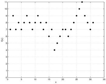
Figure 1: Function $f(x)$ of Example 5.

If $l^{0}=13$, then we can find the global minimum point $l^{*}=17$ after doing computations involving only the set of points in the set $\{1,\cdots,27\}$. Indeed the algorithm will work as follows: first it will search to the right of $13$ and it will stop at point $l^{+}=27$ because $f(27)-f(17)=7.$ The minimum value in the interval $\{13,\cdots,27\}$ is $f(17)=4.$

Then the algorithm will compare the maximum value $f(14)=8$ of $f$ in the interval $\{13,\cdots,16\}$ and since $f(14)-f(17)=4<7$, it will continue with the following step.

Now, the algorithm will search to the left of $13$ and it will stop at point $l^{-}=1$ because there is no $x\in\{1,\cdots,13\}$ satisfying $f(x)-f(17)\geq 7.$ The algorithm has computed the global minimum point $l^{*}=17,$ without considering points in the set $\{28,\cdots,31\}.$

From the definition of an Ameso($C$) optimization problem one can see that any discrete optimization problem over a finite set can be transformed into an Ameso($C$) optimization problem when $C\geq 2*(max\{f(x)\}-min\{f(x)\}),$ and its domain is an Ameso set. However, such a large $C$ is meaningless, because in order to satisfy the conditions of stopping in the above algorithm we need to check the whole domain if $C>max\{f(x)\}-min\{f(x)\}$. Therefore, it is obvious that an Ameso($C$) optimization can be preferred over other discrete optimization methods only if $C\leq max\{f(x)\}-min\{f(x)\}$. In such cases the above algorithm can narrow down the computations dramatically and as we showed in Example 5. For instance, in the Example 5 the function $f$ is an Ameso(C) problem, for any $C\geq 7.$ If we use the algorithm with $C=8$, and starting point at $l^{0}=13$, we have going though its steps as above that it will search the whole interval $\{1,\cdots,31\}$. This happened since in that case $C=8>7=max\{f(x)\}-min\{f(x)\}$. Another question that raises from the above example is which $C$ to choose since we know that if a problem is Ameso$(C)$ it is also Ameso$(aC)$, $a>0$. As we showed in Example 5, the number of computations depends on the starting point and $C$.

Notice that for an Ameso($C$) problem, $C$ is a critical value to the problem. In the algorithm, from the condition $f(l^{+})-f(l^{-})\geq C$, we can see that $C$ defines the search range. Generally, the algorithm takes more time to search the optimal solution for higher values of $C$.

2.3 Properties of multi-dimensional Ameso($C$) Pair

In this section we introduce the multi-dimensional Ameso optimization problem and we discuss its properties. Using these properties we show an algorithm for the multi-dimensional case which is based on the decomposition analysis and the one-dimensional Ameso optimization problem.

Due to that it is very complex problem, we add the following requirement to the domain of the optimization.

Assumption 1.

For the multi-dimensional problem, assume that the domain can be written as follows.

$$D^{n}=\{(x_{1},\cdots,x_{i}):x_{i}\in D_{i}\}$$ (12)

where $D_{i}$ is the domain of the $i-th$ dimension variable is an Ameso set.

For a multi-dimensional Ameso$(C)$ optimization problem: $minimize$ $f(\vec{x});$ $subject\ to$ $\vec{x}\in D^{n}$, we construct another problem: fixing the value of $j$ dimensions, denotes as $i_{1},\cdots,i_{j}$, where $i_{k}\in[1,n]$ for any $1\leq k\leq j$ satisfying $k\neq l,i_{k}\neq i_{l}$. For fixed $i_{1},...,i_{j}(n\geq j)$ we start with the following definition.

Definition 4.

1. The domain $\Delta^{j}_{i_{1},...,i_{j}}$ is the set:

   $$\Delta^{j}_{i_{1},...,i_{j}}=\{(x_{i_{1}},\cdots,x_{i_{j}}):\exists(x_{1}^{\prime},...,x_{n}^{\prime})\in D^{n}\mbox{ with }x_{i_{k}}^{\prime}=x_{i_{k}}\ ,\ k=1,...,j\}.$$

   which is the domain of $x_{i_{1}}$, $\cdots$ $x_{i,j}$ in the original domain $D^{n}.$

   Under Assumption 1, $\Delta^{j}_{i_{1},...,i_{j}}=D_{i_{1}}\times D_{i_{2}}\times\cdots\times D_{i_{j}}$.

2. The conditional domain: For fixed $x_{i_{1}}^{0},...,x_{i_{j}}^{0}$ we call the set:

   $$\Gamma_{x_{i_{1}}^{0},...,x_{i_{j}}^{0}}^{n-j}=\{(x_{1},...,x_{n})\in D^{n}:\ x_{i_{k}}=x_{i_{k}}^{0}\ ,\ k=1,...,j\}$$

   the conditional domain of $D^{n}$ given $x_{i_{1}}^{0},...,x_{i_{j}}^{0}.$

3. The conditional function: $f_{i_{1},...,i_{j}}^{*}:\Delta^{j}_{i_{1},...,i_{j}}\longrightarrow\Re$

   $$f_{i_{1},...,i_{j}}^{*}(x_{i_{1}},...,x_{i_{j}})=min_{\vec{y}\in\Gamma_{x_{i_{1}},\ldots,x_{i_{j}}}^{n-j}}f(\vec{y}).$$

4. The conditional pair of Ameso(C) pair to be the pair: $(\Delta_{i_{1},...,i_{j}}^{j},f_{i_{1},...,i_{j}}^{*}).$

We first establish the following essential property.

Property 7.

Under Assumption 1, the conditional pair $(\Delta_{i_{1},...,i_{j}}^{j},f_{i_{1},...,i_{j}}^{*})$ of an n-dimensional Ameso($C$) pair $(D^{n},f)$ is a j-dimensional Ameso($C$) pair.

Proof   At first we prove $\Delta_{i_{1},...,i_{j}}^{j}$ is an Ameso set. And $\forall(x_{i_{1}},x_{i_{2}},...,x_{i_{j}}),(y_{i_{1}},y_{i_{2}},...,y_{i_{j}})\in\Delta_{i_{1},...,i_{j}}^{j}$, we have for all $\vec{x}^{\prime}=(x_{1}^{\prime},...,x_{n}^{\prime})\in D^{n},x_{i_{k}}^{\prime}=x_{i_{k}},\forall k=1,...j$ and a vector $\vec{y}^{\prime}=(y_{1}^{\prime},...,y_{n}^{\prime})\in D^{n},y_{i_{k}}^{\prime}=y_{i_{k}},\forall k=1,...j$.

From $D^{n}$ is an Ameso set, we have $\vec{x}^{\prime},\vec{y}^{\prime}\in D^{n}\Rightarrow\left\lceil\frac{\vec{x}^{\prime}+\vec{y}^{\prime}}{2}\right\rceil,\left\lfloor\frac{\vec{x}^{\prime}+\vec{y}^{\prime}}{2}\right\rfloor\in D^{n}$.

Thus, there exists an $\left\lceil\frac{\vec{x}^{\prime}+\vec{y}^{\prime}}{2}\right\rceil\in D^{n}$ with $\left\lceil\frac{x_{i_{k}}^{\prime}+y_{i_{k}}^{\prime}}{2}\right\rceil=\left\lceil\frac{x_{i_{k}}+y_{i_{k}}}{2}\right\rceil,\forall k=1,...j$ and

$\left\lfloor\frac{\vec{x}^{\prime}+\vec{y}^{\prime}}{2}\right\rfloor\in D^{n}$ with $\left\lfloor\frac{x_{i_{k}}^{\prime}+y_{i_{k}}^{\prime}}{2}\right\rfloor=\left\lfloor\frac{x_{i_{k}}+y_{i_{k}}}{2}\right\rfloor,\forall k=1,...j$.

From $\Delta_{i_{1},...,i_{j}}^{j}=D_{i_{1}}\times D_{i_{2}}\cdots D_{i_{2}}$, we have

$$(\lceil\frac{\vec{x}_{i_{1}}+\vec{y}_{i_{1}}}{2}\rceil,...,\lceil\frac{\vec{x}_{i_{j}}+\vec{y}_{i_{j}}}{2}\rceil),(\lfloor\frac{\vec{x}_{i_{1}}+\vec{y}_{i_{1}}}{2}\rfloor,...,\lfloor\frac{\vec{x}_{i_{j}}+\vec{y}_{i_{j}}}{2}\rfloor)\in\Delta_{i_{1},...,i_{j}}^{j}$$ (13)

So $\Delta_{i_{1},...,i_{j}}^{j}$ is an Ameso set.

From the fact that function $f$ has a lower bound and the $f(\vec{x}_{0})=f_{i_{1},...,i_{j}}^{*}(x_{i_{1}},x_{i_{2}},...,x_{i_{j}})$ is in the range of $f$, the value $f(\vec{x}_{0})=f_{i_{1},...,i_{j}}^{*}(x_{i_{1}},x_{i_{2}},...,x_{i_{j}})$ must be bigger than the lower bound of $f$, for every $(x_{i_{1}},x_{i_{2}},...,x_{i_{j}})$. Thus, $f(\vec{x}_{0})=f_{i_{1},...,i_{j}}^{*}(x_{i_{1}},x_{i_{2}},...,x_{i_{j}})$ has a lower bound for each $(x_{i_{1}},x_{i_{2}},...,x_{i_{j}})$.

Next we show the third condition of the definition. For any $(x_{i_{1}},x_{i_{2}},...,x_{i_{j}}),(y_{i_{1}},y_{i_{2}},...,y_{i_{j}})\in\Delta_{i_{1},...,i_{j}}^{j}$, $\exists\vec{x}_{0}\in D^{n},\vec{y}_{0}\in D^{n}$, $f(\vec{x}_{0})=f_{i_{1},...,i_{j}}^{*}(x_{i_{1}},x_{i_{2}},...,x_{i_{j}}),f(\vec{y}_{0})=f_{i_{1},...,i_{j}}^{*}(y_{i_{1}},y_{i_{2}},...,y_{i_{j}}).$ Since $(D^{n},f)$ is an Ameso($C$) pair, we have

$\begin{array}[]{rl}&f_{i_{1},...,i_{j}}^{*}(x_{i_{1}},x_{i_{2}},...,x_{i_{j}})+f_{i_{1},...,i_{j}}^{*}(y_{i_{1}},y_{i_{2}},...,y_{i_{j}})+C\\ &=f(\vec{x}_{0})+f(\vec{y}_{0})+C\geq f(\lceil\frac{\vec{x}_{0}+\vec{y}_{0}}{2}\rceil)+f(\lfloor\frac{\vec{x}_{0}+\vec{y}_{0}}{2}\rfloor)\\ &\geq f_{i_{1},...,i_{j}}^{*}(\lceil\frac{\vec{x}_{i_{1}}+\vec{y}_{i_{1}}}{2}\rceil,...,\lceil\frac{\vec{x}_{i_{j}}+\vec{y}_{i_{j}}}{2}\rceil)+f_{i_{1},...,i_{j}}^{*}(\lfloor\frac{\vec{x}_{i_{1}}+\vec{y}_{i_{1}}}{2}\rfloor,...,\lfloor\frac{\vec{x}_{i_{j}}+\vec{y}_{i_{j}}}{2}\rfloor)\\ &\mbox{(because of (\ref{eq1}) and the definition of $f_{i_{1},...,i_{j}}^{*}(\cdot)$)}.\end{array}$

Now, we have a $j-dimensional$ Ameso set $\Delta_{i_{1},...,i_{j}}^{j}$ and a function with lower bound satisfies the condition of Ameso pair $f_{i_{1},...,i_{j}}^{*}$. Therefore, $(\Delta_{i_{1},...,i_{j}}^{j},f_{i_{1},...,i_{j}}^{*})$ is also an Ameso($C$) pair, and $f_{i_{1},...,i_{j}}^{*}$ is a $j$-dimensional function for every $(x_{i_{1}},\cdots,x_{i_{j}})\in\Delta_{i_{1},...,i_{j}}^{j}$.   $\square$

Now, using the above property we can construct an algorithm which obtains the minimum of a multi-dimensional Ameso optimization problem. Therefore, we establish the following theorem.

Theorem 4.

The solution of any Ameso optimization problem can be found using the Ameso Recursive Procedure(ARP), described in the table below.

Ameso Recursive Procedure (ARP) Input: Ameso($C$) Optimization problem: $minimize$ $f(\vec{x});$ $subject\ to$ $\vec{x}\in D^{n}$ Step 1: $A=\phi,l^{+}=0,l^{-}=0,$ select a point $l^{0}\in\Delta^{1}_{n}$,$l^{*}=l^{0},S=l^{0}$, then calculate $f_{n}^{*}(l^{0})=min_{(x_{1},\ldots,x_{n-1},l^{0})\in\Gamma_{l^{0}}^{n-1}}f(x)$  †, Step 2: Update $l^{+}=min\{x\,:\,x>l^{0},x\in\Delta^{1}_{n}-A\}$, then calculate $f_{n}^{*}(l^{+})=min_{(x_{1},\ldots,x_{n-1},l^{+})\in\Gamma_{l^{+}}^{n-1}}f(x)$ † Step 3: If $f_{n}^{*}(l^{+})-f_{n}^{*}(l^{*})\geq C$, go to step 4; If $0\leq f_{n}^{*}(l^{+})-f_{n}^{*}(l^{*})<C$, then $A=A\cup\{l^{+}\}$ go to step 2. If $f_{n}^{*}(l^{+})-f_{n}^{*}(l^{*})<0$, then $A=A\cup\{l^{+}\}$, $l^{*}=l^{+}$ go to step 2. If $\{x\,:\,x\in\Delta^{1}_{n}-A,x>l_{0}\}=\phi$, go to step 4; Step 4: Update $l^{-}$ to be any integer satisfying $f_{n}^{*}(l^{-})=max_{\{l\,:\,l\in A,l<l^{*}\}}f_{n}^{*}(l)$; If $f_{n}^{*}(l^{-})-f_{n}^{*}(l^{*})\geq C$, go to output; Step 5: Update $l^{-}=max\{x\,:\,x<l^{0},x\in\Delta^{1}_{n}-A\}$, then calculate $f_{n}^{*}(l^{-})=min_{(x_{1},\ldots,x_{n-1},l^{-})\in\Gamma_{l^{-}}^{n-1}}f(x)$ † Step 6: If $f_{n}^{*}(l^{-})-f_{n}^{*}(l^{*})\geq C$, go to output; If $0\leq f_{n}^{*}(l^{-})-f_{n}^{*}(l^{*})<C$, then $A=A\cup\{l^{-}\}$ go to step 5. If $f_{n}^{*}(l^{-})-f_{n}^{*}(l^{*})<0$, then $A=A\cup\{l^{-}\}$, $l^{*}=l^{-}$ go to step 5. If $\{x\,:\,x\in\Delta^{1}_{n}-A,x<l_{0}\}=\phi$, go to output; Output: $A$, $l^{*}$, $f_{n}^{*}(l^{*})$ †Note : the computation of $f_{n}^{*}(l^{0}),$ $f_{n}^{*}(l^{+})$ and $f_{n}^{*}(l^{-})$ above requires solving $(n-1)$-dimensional Ameso($C$) optimization problems.

Proof   The proof is easy to complete using Property 7 and Corollary 4.   $\square$

Below, we give an example with a 2-dimensional Ameso optimization problem and we implement the ARP algorithm we provided above.

Example 6: Consider the function $f(x_{1},x_{2})=88e^{\frac{1}{x_{1}}}+99e^{\frac{2}{x_{2}}}+\,:\,\frac{sin(x_{1}x_{2})}{2}\,:\,,$ and the domain $D^{2}=\{(x_{1},x_{2})\,:\,\ x_{i}=1,2,\cdots,100,\ i=1,2\}$. The problem of minimizing $f(x)$ over $D^{2}$ is a two-dimensional Ameso($1$) optimization.

Assume we pick $x_{2}=80$ as the starting point. Then $l^{0}=80$. The ARP will calculate $f_{2}^{*}(80)=min_{(x_{1},80)\in\Gamma_{80}^{1}}f(x_{1},80)=190.4220,$ where $\Gamma_{80}^{1}=\{(x_{1},x_{2})\,:\,x_{1}=1,\cdots,100;x_{2}=80\}.$ Then it will begin to search in $x_{2}$’s increasing side, i.e, $l^{+}=81,82,83,...$. It will keep on calculating $f_{2}^{*}(l^{+})=min_{(x_{1},l^{+})\in\Gamma_{l^{+}}^{1}}f(x_{1},l^{+}).$ In the end it will stop at $l^{+}=100,$ and the the minimum point in the interval $x_{2}\in\{80,\ldots,100\}$ is $f_{2}^{*}(97)=min_{(x_{1},97)\in\Gamma_{97}^{1}}f(x_{1},97)=f(97,97)=190.0093.$

Next we calculate the difference of the maximum point in the set $\{80,\cdots,96\}$ and $f_{2}^{*}(97)$, that is: $f_{2}^{*}(81)-f_{2}^{*}(97)<1=C$. Hence the ARP will next search in the direction of the decreasing side of $x_{2}(x_{2}<80),$ it will compute $f_{2}^{*}(l^{-})$ for $l^{-}=79,78,\ldots$ and it stop when $l^{-}=66$ with $f_{2}^{*}(66)-f_{2}^{*}(97)=191.1640-190.0093\geq 1.$

Now we can say that $x_{1}^{*}=97,x_{2}^{*}=97$ is a global minimum with value $f(x_{1}^{*},x_{2}^{*})=190.0093.$

We illustrate the function $f$ and the ARP technique with the following figures. In figure 2 we graph the function for all points in its domain $D^{2}.$ In figure 3 we graph the function for a smaller part of its domain. In figure 4 we plot the function only for points that were involved in our ARP technique. Note that the number of points in figure 4 is significantly smaller than the points in Figure 3 and figure 2. In figure 5 we plot the function $f_{2}^{*}(x_{2}),$ that is calculated in our ARP technique. It is an one-dimensional Ameso(1) function.

Figure 2

Figure 3

Figure 4

Figure 5

Remark 2.

In Example 6, if we choose any point $x_{2}$ greater than $65$ as starting point, then the ARP will stop after a search of all $l^{+}\in\{x_{2}+1,\cdots,100\}$ and $l^{-}\in\{x_{2}-1,\cdots,66\}$. If choose as starting point $x_{2}$ one that is smaller than $66,$ then the ARP will stop after a search of all $l^{+}\in\{x_{2}+1,\cdots,100\}$, and it will not do a search in the left side of $x_{2}$.

Remark 3.

From Examples 5 and 6, we can see that the choice of starting points and the form of the functions themselves determine the complexity of ARP. For an arbitrary integral optimization problem, if one can establish that it is an Ameso($C$) optimization for a suitable number $C,$ then one can use the ARP to find the optimal solution without necessarily searching all points in the domain.

3 An Application of Ameso(C)

In this section we consider a well known version of the knapsack problem and show it is an Ameso optimization problem. A manufacture has $W$ units of an item for shipping to its retailer. There are $N=3$ shipping options as follows. Option $i$: each package with capacity $w_{i}\in\mathbf{Z}^{+}$ and cost $c_{i}\in\mathbf{Z}^{+}$; $i=1,2,3$. It is assumed that: $w_{1}<w_{2}<w_{3}$, $c_{1}<c_{2}<c_{3}$, and $\frac{c_{1}}{w_{1}}>\frac{c_{2}}{w_{2}}>\frac{c_{3}}{w_{3}}.$

Let $z_{i}$ denote the number of packages using option $i$, where $z_{i}\in\mathbf{Z}^{+}\bigcup\{0\},$ $i=1,2$. It is assumed that any remaining capacity: $\lceil\frac{W-w_{1}z_{1}-w_{2}z_{2}}{w_{3}}\rceil$ will be assigned to Option 3.

From $\frac{c_{1}}{w_{1}}>\frac{c_{2}}{w_{2}}>\frac{c_{3}}{w_{3}}$, we have that Option 1 has the highest unit shipping cost and Option 3 is the cheapest one. The manufacturer has an external constraint of upper limit for the number of packages $z_{i}$, such as $z_{i}w_{i}\leq\frac{W}{2},\,i=1,2$.

Hence, the total cost of manufacturer can be written as

$$C(z_{1},z_{2})=c_{1}z_{1}+c_{2}z_{2}+c_{3}\lceil\frac{W-w_{1}z_{1}-w_{2}z_{2}}{w_{3}}\rceil,\,\,\,z_{i}w_{i}\leq\frac{W}{2},\,i=1,2.$$ (14)

The target is to minimize the total cost under the constraint. Therefore, the ideal structure of the objective function $C(z_{1},z_{2})$ in (14) is to be convex function or a function related to convex function in discrete version. The first discretizing convex function is the midpoint convex function which we have discussed (Property 6). One can prove that $C$ is not midpoint convex function. Therefore, we can prove that it is an Ameso optimization problem. To do that we establish the following Lemma which is necessary for proving the Ameso optimization problem cf. Theorem 5.

Lemma 6.

• If $n_{1},n_{2}\in\mathbf{Z}$, then $n_{1}+n_{2}=\lfloor\frac{n_{1}+n_{2}}{2}\rfloor+\lceil\frac{n_{1}+n_{2}}{2}\rceil$.

• If $x_{1},x_{2}\in\mathbf{R}$, then $\lceil x_{1}\rceil+\lceil x_{2}\rceil\leq\lceil x_{1}+x_{2}\rceil+1$ and

  $$\lfloor x_{1}\rfloor+\lfloor x_{2}\rfloor\leq\lfloor\frac{x_{1}+x_{2}}{2}\rfloor+\lceil\frac{x_{1}+x_{2}}{2}\rceil\leq\lceil x_{1}\rceil+\lceil x_{2}\rceil.$$

Proof  (i) If both $n_{1}$ and $n_{2}$ are even numbers (or both are odd numbers), then

$$\lfloor\frac{x_{1}+x_{2}}{2}\rfloor+\lceil\frac{x_{1}+x_{2}}{2}\rceil=\frac{x_{1}+x_{2}}{2}+\frac{x_{1}+x_{2}}{2}=x_{1}+x_{2}.$$

If $n_{1}$ is odd number and $n_{2}$ is even, then

$$\lfloor\frac{x_{1}+x_{2}}{2}\rfloor+\lceil\frac{x_{1}+x_{2}}{2}\rceil=\frac{x_{1}+x_{2}}{2}-0.5+\frac{x_{1}+x_{2}}{2}+0.5=x_{1}+x_{2}.$$

(ii) For $x_{1},x_{2}\in\mathbf{R}$, let

$$z_{1}^{-}:=\lfloor x_{1}\rfloor,\,\,a_{1}:=x_{1}-z_{1},\,\,z_{1}^{+}:=\lceil x_{1}\rceil,\,\,b_{1}:=z_{1}^{+}-x_{1};$$

$$z_{2}^{-}:=\lfloor x_{2}\rfloor,\,\,a_{2}:=x_{2}-z_{2},\,\,z_{2}^{+}:=\lceil x_{2}\rceil,\,\,b_{2}:=z_{2}^{+}-x_{2}.$$

By definition, $a_{1},b_{1},a_{2},b_{2}\geq 0$. Thus,

$$\lceil x_{1}\rceil+\lceil x_{2}\rceil =z_{1}^{+}+z_{2}^{+}=\lceil z_{1}^{+}+z_{2}^{+}-1\rceil+1$$

$$\leq\lceil z_{1}^{+}+z_{2}^{+}-1+(1-b_{1}-b_{2})\rceil+1=\lceil x_{1}+x_{2}\rceil+1.$$

The inequality comes from $-1<1-b_{1}-b_{2}$. Also,

$$\lfloor x_{1}\rfloor+\lfloor x_{2}\rfloor =z_{1}^{-}+z_{2}^{-}=\lfloor\frac{z_{1}^{-}+z_{2}^{-}}{2}\rfloor+\lceil\frac{z_{1}^{-}+z_{2}^{-}}{2}\rceil$$

$$\leq\lfloor\frac{z_{1}^{-}+z_{2}^{-}+a_{1}+a_{2}}{2}\rfloor+\lceil\frac{z_{1}^{-}+z_{2}^{-}+a_{1}+a_{2}}{2}\rceil$$

$$=\lfloor\frac{x_{1}+x_{2}}{2}\rfloor+\lceil\frac{x_{1}+x_{2}}{2}\rceil$$

$$\leq\lfloor\frac{x_{1}+x_{2}+b_{1}+b_{2}}{2}\rfloor+\lceil\frac{x_{1}+x_{2}+b_{1}+b_{2}}{2}\rceil$$

$$=\lfloor\frac{z_{1}^{+}+z_{2}^{+}}{2}\rfloor+\lceil\frac{z_{1}^{+}+z_{2}^{+}}{2}\rceil=z_{1}^{+}+z_{2}^{+}=\lceil x_{1}\rceil+\lceil x_{2}\rceil.$$

The second and fifth equality come from the result of (i). Also, the first inequality comes from $a_{1},a_{2}\geq 0$, and the second inequality comes from $b_{1},b_{2}\geq 0$. We complete the proof.   $\square$

Theorem 5.

Minimization of $C(z_{1},z_{2})$ subject to $z_{i}\in\mathbf{Z}^{+}\bigcup\{0\},$ $i=1,2$ is an Ameso($c_{3}$) optimization problem.

Proof  When $z_{i}w_{i}\leq\frac{W}{2},\,i=1,2$, we have that the domain is an Ameso set.

Next, we prove that $C$ has the necessary property to be Ameso($c_{3}$) pair. If a $(\{\mathbf{Z}^{+}\bigcup\{0\}\}^{2},C)$ is Ameso($c_{3}$) pair then minimization of $C$ is an Ameso($c_{3}$) optimization problem. For every $(z_{1},z_{2}),(z_{1}^{\prime},z_{2}^{\prime})\in\{\mathbf{Z}^{+}\bigcup\{0\}\}^{2}$, we have that

$$\,\,C(z_{1},z_{2})+C(z_{1}^{\prime},z_{2}^{\prime})+c_{3}$$

$$=c_{1}(z_{1}+z_{1}^{\prime})+c_{2}(z_{2}+z_{2}^{\prime})+c_{3}\big{(}\lceil\frac{W-w_{1}z_{1}-w_{2}z_{2}}{w_{3}}\rceil+\lceil\frac{W-w_{1}z_{1}^{\prime}-w_{2}z_{2}^{\prime}}{w_{3}}\rceil\big{)}+c_{3}$$

$$\geq c_{1}\big{(}\lfloor\frac{z_{1}+z_{1}^{\prime}}{2}\rfloor+\lceil\frac{z_{1}+z_{1}^{\prime}}{2}\rceil\big{)}+c_{2}\big{(}\lfloor\frac{z_{2}+z_{2}^{\prime}}{2}\rfloor+\lceil\frac{z_{2}+z_{2}^{\prime}}{2}\rceil\big{)}+c_{3}\big{\lceil}\frac{W-w_{1}z_{1}-w_{2}z_{2}}{w_{3}}+\frac{W-w_{1}z_{1}^{\prime}-w_{2}z_{2}^{\prime}}{w_{3}}\big{\rceil}$$

$$\,\,\,\,\,\,+c_{3}$$

$$=c_{1}\big{(}\lfloor\frac{z_{1}+z_{1}^{\prime}}{2}\rfloor+\lceil\frac{z_{1}+z_{1}^{\prime}}{2}\rceil\big{)}+c_{2}\big{(}\lfloor\frac{z_{2}+z_{2}^{\prime}}{2}\rfloor+\lceil\frac{z_{2}+z_{2}^{\prime}}{2}\rceil\big{)}+c_{3}\big{\lceil}\frac{2W-w_{1}(z_{1}+z_{1}^{\prime})-w_{2}(z_{2}+z_{2}^{\prime})}{w_{3}}\big{\rceil}+c_{3}$$

$$=c_{1}\big{(}\lfloor\frac{z_{1}+z_{1}^{\prime}}{2}\rfloor+\lceil\frac{z_{1}+z_{1}^{\prime}}{2}\rceil\big{)}+c_{2}\big{(}\lfloor\frac{z_{2}+z_{2}^{\prime}}{2}\rfloor+\lceil\frac{z_{2}+z_{2}^{\prime}}{2}\rceil\big{)}$$

$$\,\,\,\,\,\,\,\,\,\,\,\,\,\,\,\,\,\,\,\,\,\,\,\,\,\,\,\,\,\,\,\,\,\,\,\,\,\,\,\,\,\,\,\,\,\,+c_{3}\bigg{(}\big{\lceil}\frac{2W-w_{1}\big{(}\lfloor\frac{z_{1}+z_{1}^{\prime}}{2}\rfloor+\lceil\frac{z_{1}+z_{1}^{\prime}}{2}\rceil\big{)}-w_{2}\big{(}\lfloor\frac{z_{2}+z_{2}^{\prime}}{2}\rfloor+\lceil\frac{z_{2}+z_{2}^{\prime}}{2}\rceil\big{)}}{w_{3}}\big{\rceil}+1\bigg{)}$$

$$=c_{1}\big{(}\lfloor\frac{z_{1}+z_{1}^{\prime}}{2}\rfloor+\lceil\frac{z_{1}+z_{1}^{\prime}}{2}\rceil\big{)}+c_{2}\big{(}\lfloor\frac{z_{2}+z_{2}^{\prime}}{2}\rfloor+\lceil\frac{z_{2}+z_{2}^{\prime}}{2}\rceil\big{)}$$

$$\,\,\,\,\,\,\,\,\,\,\,\,\,\,\,\,\,\,\,\,\,\,\,\,\,\,\,\,\,\,\,\,\,\,\,\,\,\,\,\,\,\,\,\,\,\,+c_{3}\bigg{(}\big{\lceil}\frac{W-w_{1}\lfloor\frac{z_{1}+z_{1}^{\prime}}{2}\rfloor-w_{2}\lfloor\frac{z_{2}+z_{2}^{\prime}}{2}\rfloor}{w_{3}}+\frac{W-w_{1}\lceil\frac{z_{1}+z_{1}^{\prime}}{2}\rceil-w_{2}\lceil\frac{z_{2}+z_{2}^{\prime}}{2}\rceil}{w_{3}}\big{\rceil}+1\bigg{)}$$

$$\geq c_{1}\big{(}\lfloor\frac{z_{1}+z_{1}^{\prime}}{2}\rfloor+\lceil\frac{z_{1}+z_{1}^{\prime}}{2}\rceil\big{)}+c_{2}\big{(}\lfloor\frac{z_{2}+z_{2}^{\prime}}{2}\rfloor+\lceil\frac{z_{2}+z_{2}^{\prime}}{2}\rceil\big{)}$$

$$\,\,\,\,\,\,\,\,\,\,\,\,\,\,\,\,\,\,\,\,\,\,\,\,\,\,\,\,\,\,\,\,\,\,\,\,\,\,\,\,\,\,\,\,\,\,+c_{3}\bigg{[}\big{\lceil}\frac{W-w_{1}\lfloor\frac{z_{1}+z_{1}^{\prime}}{2}\rfloor-w_{2}\lfloor\frac{z_{2}+z_{2}^{\prime}}{2}\rfloor}{w_{3}}\big{\rceil}+\big{\lceil}\frac{W-w_{1}\lceil\frac{z_{1}+z_{1}^{\prime}}{2}\rceil-w_{2}\lceil\frac{z_{2}+z_{2}^{\prime}}{2}\rceil}{w_{3}}\big{\rceil}\bigg{]}$$

$$=C(\lfloor\frac{z_{1}+z_{1}^{\prime}}{2}\rfloor,\lfloor\frac{z_{2}+z_{2}^{\prime}}{2}\rfloor)+C(\lceil\frac{z_{1}+z_{1}^{\prime}}{2}\rceil,\lceil\frac{z_{2}+z_{2}^{\prime}}{2}\rceil).$$

The first inequality comes from the fact that $\lceil x_{1}+x_{2}\rceil\leq\lceil x_{1}\rceil+\lceil x_{2}\rceil$ for every $x_{1},x_{2}\in\mathbf{R}$. Also, the third equality and the second inequality come from Lemma 6. Thus, the proof is complete.   $\square$

We have established that the problem is an Ameso($c_{3}$) optimization problem. This work can be easily generalized to the case of $k$ possible shipping options.

4 Conclusions

In this paper we introduced the class of Ameso($C$) optimization problems and established the following:

1. For one-dimensional Ameso optimization problems there are simple to verify optimality conditions at any optimal point cf. Theorems 1,2,3 and corresponding corollaries.

2. The conditional pair of Ameso($C$) pair is still an Ameso($C$) pair cf. Property 5.

3. We have constructed the ARP algorithm that solves multi-dimensional Ameso optimization problems without necessarily performing complete enumeration cf. ARP.

We showed that one can establish that a problem is Ameso($C$) optimization in the same way one proves convexity or midpoint convexity. Further, one can see that an Ameso(C) optimization is a relaxed convex model, since convex cases correspond to an Ameso(0) optimization problem.

As we mentioned in Section 2.2, in a general setting it is not possible establish bounds for the constant $C$. However, in specific problems such as in Section 3, a problem specific bound for the constant $C$ can be obtained by direct model analysis. Further, for models with functions where it is not possible to prove convexity or midpoint convexity it may still be possible to show that the more relaxed property of the Ameso(1) optimization holds. To do that is easier than to prove convexity and at the same time there is the ARP algorithm that can compute the minimum point without requiring complete enumeration.

Acknowledgments We acknowledge support for this work from the National Science Foundation, NSF grant CMMI-16-62629.

References

- [1] Ahuja, R.K., Magnanti, T.L., Orlin, J.B. (1993). “Network Flows—Theory, Algorithms and Applications”, Prentice-Hall, Englewood Cliffs.
- [2] Bertsekas, D. P. and Tsitsiklis, J. N. (2003). “Parallel and Distributed Computation: Numerical Methods”, LIDS Technical Reports, MIT, Boston Ma.
- [3] Bertsimas, D.J. and van Ryzin, G.J. (1993). “Stochastic and Dynamic Vehicle Routing with General Interarrival and Service Time Distributions”, Advances in Applied Probability, 25, pp. 947-978.
- [4] Bertsimas, D.J. and van Ryzin, G.J. (1990). “An Asymptotic Determination of the Minimum Spanning Tree and Minimum Matching Constants in Geometrical Probability,” Operations Research Letters, 9, pp. 223-231.
- [5] De Loera, J.A., Hemmecke, R., Koppe, M. (2013). “Algebraic and Geometric Ideas in the Theory of Discrete Optimization”, SIAM, Philadelphia.
- [6] Denardo, E. V. (1982). “Dynamic Programming: Models and Applications”, NJ, Englewood Cliffs:Prentice-Hall.
- [7] Denardo, E. V., Huberman, G. and Rothblum, U. G. (1982). “Optimal Locations on a Line Are Interleaved”, Operations Research, 30, pp. 745-759.
- [8] Hemmecke, R., Koppe, M., Lee, J., Weismantel, R. (2010). “Nonlinear integer programming”, In: Junger, M., et al. (eds.) 50 Years of Integer Programming 1958-2008: From The Early Years and State-of-the-Art, Chapter 15, pp. 561-618, Springer, Berlin.
- [9] Gilmore, P.C. ,and Gomony, R. E. (1961). “A linear programming approach to the cutting stock problem”, Operations Research, 9, pp. 849-859.
- [10] Gilmore, P.C. ,and Gomony, R. E. (1963). “A linear programming approach to the cutting stock problem. Part II.”, Operations Research, 11, pp. 863-888.
- [11] Gilmore, P.C. ,and Gomony, R. E.(1966). “The theory and computation of knapsack functions”, Operations Research, 14, pp. 1045-1074.
- [12] Gittins, J., Glazebrook, K., and Weber, R. (2011). “ Multi-armed bandit allocation indices”, John Wiley & Sons.
- [13] Hemmecke, R., Koppe, M., Lee, J., Weismantel, R. (2010). “Nonlinear integer programming”, In: Junger, M., et al. (eds.) 50 Years of Integer Programming 1958-2008: From The Early Years and State-of-the-Art, Chapter 15, pp. 561-618, Springer, Berlin.
- [14] Hochbaum, D.S. (2007). “Complexity and algorithms for nonlinear optimization problems”, Annals of Operations Research 153, pp. 257-296.
- [15] Hochbaum, D.S., Shanthikumar, J.G. (1990). “Convex separable optimization is not much harder than linear optimization”, Journal of the Association for Computing Machinery 37, pp. 843-862.
- [16] Ibaraki, T., Katoh, N. (1988). “Resource Allocation Problems: Algorithmic Approaches”, MIT Press, Boston.
- [17] Iwata, S., Moriguchi, S., Murota, K. (2005). “A capacity scaling algorithm for M-convex sub- modular flow”, Mathematical Programming 103, pp.181-202.
- [18] Iwata, S., Shigeno, M. (2002). “Conjugate scaling algorithm for Fenchel-type duality in discrete convex optimization”, SIAM Journal on Optimization 13, 204-211.
- [19] Katehakis, M. N., and Veinott Jr, A. F. (1987). “The multi-armed bandit problem: decomposition and computation”, Mathematics of Operations Research, 12(2), 262-268.
- [20] Katoh, N., Shioura, A., Ibaraki, T. (2013). “Resource allocation problems”, In: Pardalos, P.M., Du, D.-Z., Graham, R.L. (eds.) Handbook of Combinatorial Optimization, 2nd ed., Vol. 5, pp. 2897-2988, Springer, Berlin.
- [21] Peter J. Kolesar (1967).“A Branch and Bound Algorithm for the Knapsack Problem”, Management Science, 13(9), pp.723-735.
- [22] Lee, J., Leyffer, S. (2012), “Mixed Integer Nonlinear Programming”, The IMA Volumes in Mathematics and its Applications 154, Springer, Berlin.
- [23] Lewis, H. R and Papadimitriou, C. H (1998). “ Elements of the Theory of Computation”, ACM Press, New York.
- [24] Moriguchi, S., Murota, K., Tamura, A., and Tardella, F. (2017). “Discrete Midpoint Convexity”, https://arxiv.org/pdf/1708.04579.pdf.
- [25] Onn, S. (2010). “Nonlinear Discrete Optimization: An Algorithmic Theory”, European Mathematical Society, Zurich.
- [26] Papadimitriou, C. H. and Steiglitz, K. (1982). “Combinatorial Optimization: Algorithms and Complexity”, Prentice-Hall.
- [27] Papadimitriou , C. H. and Yannakakis, M. (1982). “ The complexity of facets (and some facets of complexity)”, Annual ACM Symposium on Theory of Computing archive Proceedings of the fourteenth annual ACM symposium on Theory of computing, San Francisco, California, United States, pp. 255 - 260.
- [28] Ross, K. W., and Tsang, D. H. K. (1989). “The stochastic knapsack problem”, IEEE Transactions on Communications, 37(7), pp. 740-747.
- [29] Shapiro, J. F., and H. M. Wanger, H.M. (1967). “A finite renewal algorithm for the knapsack and turnpike models”, Operations Research, 15, pp. 319-341.
- [30] Topkis D. M. (1978). “Minimizing a Submodular Function on a Lattice”, Operations Research, 26, pp. 305-321.
- [31] Yannakakis M. (1982). “The complexity of the partial order dimension problem”, SIAM J. Alg. Dis. Meth.,3, pp. 351-370.
- [32] Yannakakis M. (1990). “The analysis of local search problems modified greedy heuristic for the set covering problem and their heuristics”, STAG’S -90, pp. 298-311.
- [33] Zipkin P. (2016). “Some specially structured assemble-to-order systems”, Operations Research Letters, 44, pp. 136-142.