Multigrid methods for saddle point problems: Karush-Kuhn-Tucker systems

Abstract.

We construct multigrid methods for an elliptic distributed optimal control problem that are robust with respect to a regularization parameter. We prove the uniform convergence of the $W$-cycle algorithm and demonstrate the performance of $V$-cycle and $W$-cycle algorithms in two and three dimensions through numerical experiments.

1. Introduction

Let $\Omega$ be a bounded convex polygonal domain in $\mathbb{R}^{d}$ ($d=2,3$), $y_{d}\in{L_{2}(\Omega)}$, $\beta$ be a positive constant and $(\cdot,\cdot)_{L_{2}(\Omega)}$ be the inner product of ${L_{2}(\Omega)}$ (or $[{L_{2}(\Omega)}]^{d}$). The optimal control problem is to find

(1.1) $$(\bar{y},\bar{u})=\operatorname*{argmin}_{(y,u)\in K}\left[\frac{1}{2}\|y-y_{d}\|^{2}_{{L_{2}(\Omega)}}+\frac{\beta}{2}\|u\|^{2}_{L_{2}(\Omega)}\right],$$

where $(y,u)$ belongs to $K\subset H^{1}_{0}(\Omega)\times{L_{2}(\Omega)}$ if and only if

(1.2) $$(\nabla y,\nabla v)_{L_{2}(\Omega)}=(u,v)_{L_{2}(\Omega)}\quad\forall\,v\in H^{1}_{0}(\Omega).$$

Here and throughout the paper we will follow the standard notation for differential operators, function spaces and norms that can be found for example in [10, 8].

The optimal control problem (1.1)–(1.2) has a unique solution characterized by the following system of equations (cf. [16, 22]):

(1.3a) $$(\nabla\bar{p},\nabla q)_{L_{2}(\Omega)} =(\bar{y}-y_{d},q)_{L_{2}(\Omega)} \forall\,q\in{H^{1}_{0}(\Omega)},$$

(1.3b) $$\bar{p}+\beta\bar{u} =0,$$

(1.3c) $$(\nabla\bar{y},\nabla z)_{L_{2}(\Omega)} =(\bar{u},z)_{L_{2}(\Omega)} \forall\,z\in{H^{1}_{0}(\Omega)},$$

where $\bar{p}$ is the (optimal) adjoint state. After eliminating $\bar{u}$, we have a symmetric saddle point problem

(1.4a) $$(\nabla\bar{p},\nabla q)_{L_{2}(\Omega)}-(\bar{y},q)_{L_{2}(\Omega)} =-(y_{d},q)_{L_{2}(\Omega)} \forall\,q\in{H^{1}_{0}(\Omega)},$$

(1.4b) $$-(\bar{p},z)_{L_{2}(\Omega)}-\beta(\nabla\bar{y},\nabla z)_{L_{2}(\Omega)} =0 \forall\,z\in{H^{1}_{0}(\Omega)}.$$

Note that the system (1.4) is unbalanced with respect to $\beta$ since it only appears in (1.4b). This can be remedied by the following change of variables:

(1.5) $$\bar{p}=\beta^{\frac{1}{4}}\tilde{p}\quad\text{and}\quad\bar{y}=\beta^{-\frac{1}{4}}\tilde{y}.$$

The resulting saddle point problem is

(1.6a) $$\beta^{\frac{1}{2}}(\nabla\tilde{p},\nabla q)_{L_{2}(\Omega)}-(\tilde{y},q)_{L_{2}(\Omega)} =-\beta^{\frac{1}{4}}(y_{d},q)_{L_{2}(\Omega)} \forall\,{q}\in{H^{1}_{0}(\Omega)},$$

(1.6b) $$-(\tilde{p},{z})_{L_{2}(\Omega)}-\beta^{\frac{1}{2}}(\nabla\tilde{y},\nabla{z})_{L_{2}(\Omega)} =0 \forall\,{z}\in{H^{1}_{0}(\Omega)}.$$

The saddle point problem (1.6) can be discretized by a $P_{1}$ finite element method. Our goal is to design multigrid methods for the resulting discrete saddle point problem whose performance is independent of the regularization parameter $\beta$. The key idea is to use a post-smoother that can be interpreted as a Richardson iteration for a symmetric positive definite (SPD) problem that has the same solution as the saddle point problem. Consequently we can exploit the well-known multigrid theory for SPD problems [15, 17, 4] in our convergence analysis. This idea has previously been applied to other saddle point problems in [5, 6, 7].

Our multigrid methods belong to the class of all-at-once methods where all the unknowns in (1.4) are solved simultaneously (cf. [2, 13, 20, 3, 21] and the references therein). Multigrid methods that are robust with respect to $\beta$ can also be found in the papers [20, 21]. The differences are in the construction of the smoothers and in the norms that measure the convergence of the multigrid algorithms. The smoothing steps in [20, 21] are computationally less expensive than the one in the current paper, which requires solving (approximately) a diffusion-reaction problem (which however does not affect the $O(n)$ complexity). The trade-off is that the convergence of the multigrid algorithm in this paper is expressed in terms of the natural energy norm for the continuous problem, while the norms in [20, 21] are different from the energy norm. A related consequence is that the $W$-cycle multigrid algorithms in [20, 21] cannot take advantage of post-smoothing and hence their contraction numbers decay at the rate of $O(m^{-1/2})$, where $m$ is the number of pre-smoothing steps, while the contraction number for our symmetric $W$-cycle multigrid algorithm decays at the rate of $O(m^{-1})$, where $m$ is the number of pre-smoothing and post-smoothing steps.

The rest of the paper is organized as follows. We analyze the saddle point problem (1.6) and the $P_{1}$ finite element method in Section 2 and introduce the multigrid algorithms in Section 3. We derive smoothing and approximation properties in Section 4 that are the key ingredients for the convergence analysis of the $W$-cycle algorithm in Section 5. Numerical results are presented in Section 6 and we end with some concluding remarks in Section 7.

Throughout this paper, we use $C$ (with or without subscripts) to denote a generic positive constant that is independent of $\beta$ and any mesh parameter. Also to avoid the proliferation of constants, we use the notation $A\lesssim B$ (or $A\gtrsim B$) to represent $A\leq\text{(constant)}B$, where the (hidden) positive constant is independent of $\beta$ and any mesh parameter. The notation $A\approx B$ is equivalent to $A\lesssim B$ and $B\lesssim A$.

2. A $P_{1}$ Finite Element Method

We can express (1.6) concisely as

(2.1) $$\mathcal{B}((\tilde{p},\tilde{y}),({q},{z}))=-\beta^{\frac{1}{4}}(y_{d},{q})_{L_{2}(\Omega)}\qquad\forall\,({q},{z})\in{H^{1}_{0}(\Omega)}\times{H^{1}_{0}(\Omega)},$$

where

(2.2) $$\mathcal{B}((p,y),(q,z))=\beta^{\frac{1}{2}}(\nabla p,\nabla q)_{L_{2}(\Omega)}-(y,q)_{L_{2}(\Omega)}-(p,z)_{L_{2}(\Omega)}-\beta^{\frac{1}{2}}(\nabla y,\nabla z)_{L_{2}(\Omega)}.$$

2.1. Properties of $\mathcal{B}$

We will analyze the bilinear form $\mathcal{B}(\cdot,\cdot)$ in terms of the weighted $H^{1}$ norm $\|\cdot\|_{H^{1}_{\beta}(\Omega)}$ defined by

(2.3) $$\|v\|^{2}_{H^{1}_{\beta}(\Omega)}=\|v\|^{2}_{L_{2}(\Omega)}+\beta^{\frac{1}{2}}|v|^{2}_{H^{1}(\Omega)}\qquad\forall\,v\in{H^{1}(\Omega)}.$$

Let $(p,y)\in{H^{1}(\Omega)}\times{H^{1}(\Omega)}$ be arbitrary. It follows immediately from (2.2), (2.3) and the Cauchy-Schwarz inequality that

(2.4) $$\mathcal{B}((p,y),(q,z))\leq(\|p\|^{2}_{H^{1}_{\beta}(\Omega)}+\|y\|^{2}_{H^{1}_{\beta}(\Omega)})^{\frac{1}{2}}(\|q\|^{2}_{H^{1}_{\beta}(\Omega)}+\|z\|^{2}_{H^{1}_{\beta}(\Omega)})^{\frac{1}{2}}.$$

Moreover, a direct calculation shows that

$$\mathcal{B}((p,y),(p-y,-y-p)) =\beta^{\frac{1}{2}}(\nabla p,\nabla(p-y))_{L_{2}(\Omega)}-(y,p-y)_{L_{2}(\Omega)}$$

(2.5) $$\hskip 30.0pt+(p,y+p)_{L_{2}(\Omega)}+\beta^{\frac{1}{2}}(\nabla y,\nabla(y+p))_{L_{2}(\Omega)}$$

$$=\|p\|_{H^{1}_{\beta}(\Omega)}^{2}+\|y\|_{H^{1}_{\beta}(\Omega)}^{2},$$

and we also have, by the parallelogram law,

(2.6) $$\|p-y\|_{H^{1}_{\beta}(\Omega)}^{2}+\|-y-p\|_{H^{1}_{\beta}(\Omega)}^{2} =2(\|p\|_{H^{1}_{\beta}(\Omega)}^{2}+\|y\|_{H^{1}_{\beta}(\Omega)}^{2}).$$

It follows from (2.4)–(2.6) that

$$\,(\|p\|^{2}_{H^{1}_{\beta}(\Omega)}+\|y\|^{2}_{H^{1}_{\beta}(\Omega)})^{\frac{1}{2}}$$

(2.7) $$\geq \,\sup_{(q,z)\in{H^{1}_{0}(\Omega)}\times{H^{1}_{0}(\Omega)}}\frac{\mathcal{B}((p,y),(q,z))}{(\|q\|^{2}_{H^{1}_{\beta}(\Omega)}+\|z\|^{2}_{H^{1}_{\beta}(\Omega)})^{\frac{1}{2}}}$$

$$\geq \,2^{-\frac{1}{2}}(\|p\|^{2}_{H^{1}_{\beta}(\Omega)}+\|y\|^{2}_{H^{1}_{\beta}(\Omega)})^{\frac{1}{2}} \quad\forall\,(p,y)\in{H^{1}_{0}(\Omega)}\times{H^{1}_{0}(\Omega)}.$$

2.2. The Discrete Problem

Let $\mathcal{T}_{h}$ be a simplicial triangulation of $\Omega$ and $V_{h}\subset{H^{1}_{0}(\Omega)}$ be the $P_{1}$ finite element space associated with $\mathcal{T}_{h}$. The $P_{1}$ finite element method for (2.1) is to find $(\tilde{p}_{h},\tilde{y}_{h})\in V_{h}\times V_{h}$ such that

(2.8) $$\mathcal{B}((\tilde{p}_{h},\tilde{y}_{h}),({q}_{h},{z}_{h}))=-\beta^{\frac{1}{4}}(y_{d},{q}_{h})_{L_{2}(\Omega)}\qquad\forall\,({q}_{h},{z}_{h})\in V_{h}\times V_{h}.$$

For the convergence analysis of the multigrid algorithms, it is necessary to consider a more general problem: Find $(p,y)\in{H^{1}_{0}(\Omega)}\times{H^{1}_{0}(\Omega)}$ such that

(2.9) $$\mathcal{B}((p,y),(q,z))=(f,q)_{L_{2}(\Omega)}+(g,z)_{L_{2}(\Omega)}\qquad\forall\,(q,z)\in{H^{1}_{0}(\Omega)}\times{H^{1}_{0}(\Omega)},$$

where $f,g\in{L_{2}(\Omega)}$. The unique solvability of (2.9) follows immediately from (2.1).

The $P_{1}$ finite element method for (2.9) is to find $(p_{h},y_{h})\in V_{h}\times V_{h}$ such that

(2.10) $$\mathcal{B}((p_{h},y_{h}),(q_{h},z_{h}))=(f,q_{h})_{L_{2}(\Omega)}+(g,z_{h})_{L_{2}(\Omega)}\qquad\forall\,(q_{h},z_{h})\in V_{h}\times V_{h}.$$

Note that (2.4)–(2.6) also yield the following analog of (2.1):

$$\,(\|p_{h}\|^{2}_{H^{1}_{\beta}(\Omega)}+\|y_{h}\|^{2}_{H^{1}_{\beta}(\Omega)})^{\frac{1}{2}}$$

(2.11) $$\geq \,\sup_{(q_{h},z_{h})\in V_{h}\times V_{h}}\frac{\mathcal{B}((p_{h},y_{h}),(q_{h},z_{h}))}{(\|q_{h}\|^{2}_{H^{1}_{\beta}(\Omega)}+\|z_{h}\|^{2}_{H^{1}_{\beta}(\Omega)})^{\frac{1}{2}}}$$

$$\geq \,2^{-\frac{1}{2}}(\|p_{h}\|^{2}_{H^{1}_{\beta}(\Omega)}+\|y_{h}\|^{2}_{H^{1}_{\beta}(\Omega)})^{\frac{1}{2}} \quad\forall\,(p_{h},y_{h})\in V_{h}\times V_{h}.$$

Therefore the discrete problem (2.10) is uniquely solvable.

2.3. Error Estimates for (2.9)

From (2.4), (2.2) and the saddle point theory [1, 9, 24], we have the following quasi-optimal error estimate.

Lemma 2.1.

Let $(p,y)$ $($resp., $(p_{h},y_{h}))$ be the solution of (2.9) $(resp.,\eqref{eq:DGP})$. We have

(2.12) $$\|p-p_{h}\|_{H^{1}_{\beta}(\Omega)}^{2}+\|y-y_{h}\|_{H^{1}_{\beta}(\Omega)}^{2}\leq 2\inf_{(q_{h},z_{h})\in V_{h}\times V_{h}}\big{(}\|p-q_{h}\|_{H^{1}_{\beta}(\Omega)}^{2}+\|y-z_{h}\|_{H^{1}_{\beta}(\Omega)}^{2}\big{)}.$$

In order to convert (2.12) into a concrete error estimate, we need the regularity of the solution of (2.9).

Lemma 2.2.

The solution $(p,y)$ of (2.9) belongs to $H^{2}(\Omega)\times H^{2}(\Omega)$ and we have

(2.13) $$\|\beta^{\frac{1}{2}}p\|_{H^{2}(\Omega)}+\|\beta^{\frac{1}{2}}y\|_{H^{2}(\Omega)}\leq C_{\Omega}(\|f\|_{L_{2}(\Omega)}+\|g\|_{L_{2}(\Omega)}).$$

Proof.

We can write (2.9) as

$$(\nabla(\beta^{\frac{1}{2}}p),\nabla q)_{L_{2}(\Omega)} =(y+f,q)_{L_{2}(\Omega)} \forall\,q\in{H^{1}_{0}(\Omega)},$$

$$(\nabla(\beta^{\frac{1}{2}}y),\nabla z)_{L_{2}(\Omega)} =(-p-g,z)_{L_{2}(\Omega)}. \forall\,z\in{H^{1}_{0}(\Omega)},$$

and hence, by the elliptic regularity theory for convex domains [14, 11],

(2.14a) $$\|\beta^{\frac{1}{2}}p\|_{H^{2}(\Omega)} \leq C_{\Omega}(\|y\|_{L_{2}(\Omega)}+\|f\|_{L_{2}(\Omega)}),$$

(2.14b) $$\|\beta^{\frac{1}{2}}y\|_{H^{2}(\Omega)} \leq C_{\Omega}(\|p\|_{L_{2}(\Omega)}+\|g\|_{L_{2}(\Omega)}).$$

From (2.3), (2.1) and (2.9) we also have

(2.15) $$\|p\|_{L_{2}(\Omega)}^{2}+\|y\|_{L_{2}(\Omega)}^{2}\leq 2(\|f\|_{L_{2}(\Omega)}^{2}+\|g\|_{L_{2}(\Omega)}^{2}).$$

The estimate (2.13) follows from (2.14) and (2.15). ∎

We can now derive concrete error estimates for the $P_{1}$ finite element method for (2.9).

Lemma 2.3.

Let $(p,y)$ $($resp., $(p_{h},y_{h}))$ be the solution of (2.9) $(resp.,\eqref{eq:DGP})$. We have

(2.16) $$\|p-p_{h}\|_{H^{1}_{\beta}(\Omega)}+\|y-y_{h}\|_{H^{1}_{\beta}(\Omega)} \leq C(1+{\beta}^{\frac{1}{2}}h^{-2})^{\frac{1}{2}}\beta^{-\frac{1}{2}}h^{2}(\|f\|_{L_{2}(\Omega)}+\|g\|_{L_{2}(\Omega)}),$$

(2.17) $$\|p-p_{h}\|_{L_{2}(\Omega)}+\|y-y_{h}\|_{L_{2}(\Omega)} \leq C(1+{\beta}^{\frac{1}{2}}h^{-2})\beta^{-1}h^{4}(\|f\|_{L_{2}(\Omega)}+\|g\|_{L_{2}(\Omega)}),$$

where the positive constant $C$ is independent of $\beta$ and $h$.

Proof.

Let $\Pi_{h}:H^{2}(\Omega)\cap{H^{1}_{0}(\Omega)}\longrightarrow V_{h}$ be the nodal interpolation operator. We have the following standard interpolation error estimate [10, 8]:

(2.18) $$\|\zeta-\Pi_{h}\zeta\|_{L_{2}(\Omega)}+h|\zeta-\Pi_{h}\zeta|_{H^{1}(\Omega)}\leq Ch^{2}|\zeta|_{H^{2}(\Omega)}\qquad\forall\,\zeta\in H^{2}(\Omega)\cap{H^{1}_{0}(\Omega)},$$

where the positive constant $C$ only depends on the shape regularity of $\mathcal{T}_{h}$.

The estimate (2.16) follows from (2.3), (2.12), (2.13) and (2.18):

$$\|p-p_{h}\|_{H^{1}_{\beta}(\Omega)}^{2}+\|y-y_{h}\|_{H^{1}_{\beta}(\Omega)}^{2}\leq 2\big{(}\|p-\Pi_{h}p\|_{H^{1}_{\beta}(\Omega)}^{2}+\|y-\Pi_{h}y\|_{H^{1}_{\beta}(\Omega)}^{2}\big{)}$$

$$\hskip 40.0pt\leq 2\big{(}\|p-\Pi_{h}p\|_{L_{2}(\Omega)}^{2}+\beta^{\frac{1}{2}}|p-\Pi_{h}p|_{H^{1}(\Omega)}^{2}+\|y-\Pi_{h}y\|_{L_{2}(\Omega)}^{2}+\beta^{\frac{1}{2}}|y-\Pi_{h}y|_{H^{1}(\Omega)}^{2}\big{)}$$

$$\hskip 40.0pt\leq C(\beta^{-1}h^{4}+\beta^{-\frac{1}{2}}h^{2})(\|f\|_{L_{2}(\Omega)}^{2}+\|g\|_{L_{2}(\Omega)}^{2})$$

$$\hskip 40.0pt=C(1+\beta^{\frac{1}{2}}h^{-2})\beta^{-1}h^{4}(\|f\|_{L_{2}(\Omega)}^{2}+\|g\|_{L_{2}(\Omega)}^{2}).$$

The estimate (2.17) is established by a duality argument. Let $(\xi,\theta)\in{H^{1}_{0}(\Omega)}\times{H^{1}_{0}(\Omega)}$ be defined by

(2.19) $$\mathcal{B}((\xi,\theta),(q,z))=(p-p_{h},q)_{L_{2}(\Omega)}+(y-y_{h},z)_{L_{2}(\Omega)}\qquad\forall\,(q,z)\in{H^{1}_{0}(\Omega)}\times{H^{1}_{0}(\Omega)}.$$

We have, by (2.4), Lemma 2.2 (applied to (2.19)), (2.18), (2.19) and Galerkin orthogonality,

$$\|p-p_{h}\|^{2}_{L_{2}(\Omega)}+\|y-y_{h}\|^{2}_{L_{2}(\Omega)}=(p-p_{h},p-p_{h})_{L_{2}(\Omega)}+(y-y_{h},y-y_{h})_{L_{2}(\Omega)}$$

$$\hskip 40.0pt=\mathcal{B}((\xi,\theta),(p-p_{h},y-y_{h}))$$

$$\hskip 40.0pt=\mathcal{B}((\xi-\Pi_{h}\xi,\theta-\Pi_{h}\theta),(p-p_{h},y-y_{h}))$$

$$\hskip 40.0pt\leq(\|\xi-\Pi_{h}\xi\|^{2}_{H^{1}_{\beta}(\Omega)}+\|\theta-\Pi_{h}\theta\|^{2}_{H^{1}_{\beta}(\Omega)})^{\frac{1}{2}}(\|p-p_{h}\|^{2}_{H^{1}_{\beta}(\Omega)}+\|y-y_{h}\|^{2}_{H^{1}_{\beta}(\Omega)})^{\frac{1}{2}}$$

$$\hskip 40.0pt\leq C(1+{\beta}^{\frac{1}{2}}h^{-2})^{\frac{1}{2}}\beta^{-\frac{1}{2}}h^{2}(\|p-p_{h}\|_{L_{2}(\Omega)}^{2}+\|y-y_{h}\|_{L_{2}(\Omega)}^{2})^{\frac{1}{2}}$$

$$\hskip 70.0pt\times(\|p-p_{h}\|^{2}_{H^{1}_{\beta}(\Omega)}+\|y-y_{h}\|^{2}_{H^{1}_{\beta}(\Omega)})^{\frac{1}{2}},$$

which together with (2.16) implies (2.17). ∎

2.4. A $\bm{P_{1}}$ Finite Element Method for (1.4)

The $P_{1}$ finite element method for (1.4) is to find $(\bar{p}_{h},\bar{y}_{h})\in V_{h}\times V_{h}$ such that

(2.20a) $$(\nabla\bar{p}_{h},\nabla q_{h})_{L_{2}(\Omega)}-(\bar{y}_{h},q_{h})_{L_{2}(\Omega)} =-(y_{d},q_{h})_{L_{2}(\Omega)} \forall\,q_{h}\in V_{h},$$

(2.20b) $$-(\bar{p}_{h},z_{h})_{L_{2}(\Omega)}-\beta(\nabla\bar{y}_{h},\nabla z_{h})_{L_{2}(\Omega)} =0 \forall\,z_{h}\in V_{h},$$

which is equivalent to (2.8) under the change of variables

(2.21) $$\bar{p}_{h}=\beta^{\frac{1}{4}}\tilde{p}_{h}\quad\text{and}\quad\bar{y}_{h}=\beta^{-\frac{1}{4}}\tilde{y}_{h}.$$

Applying the results in Section 2.3 to (2.1) and (2.8), we arrive at the following error estimates through the change of variables (1.5) and (2.21).

Lemma 2.4.

Let $(\bar{p},\bar{y})$ $($resp., $(\bar{p}_{h},\bar{y}_{h}))$ be the solution of (1.4) $($resp., (2.20)$)$. We have

$$\|\bar{p}-\bar{p}_{h}\|_{H^{1}_{\beta}(\Omega)}+\beta^{\frac{1}{2}}\|\bar{y}-\bar{y}_{h}\|_{H^{1}_{\beta}(\Omega)} \leq C(1+{\beta}^{\frac{1}{2}}h^{-2})^{\frac{1}{2}}h^{2}\|y_{d}\|_{L_{2}(\Omega)},$$

$$\|\bar{p}-\bar{p}_{h}\|_{L_{2}(\Omega)}+\beta^{\frac{1}{2}}\|\bar{y}-\bar{y}_{h}\|_{L_{2}(\Omega)} \leq C(1+{\beta}^{\frac{1}{2}}h^{-2})\beta^{-\frac{1}{2}}h^{4}\|y_{d}\|_{L_{2}(\Omega)},$$

where the positive constant $C$ is independent of $\beta$ and $h$.

According to Lemma 2.4, the performance of the $P_{1}$ finite element method defined by (2.20) will deteriorate as $\beta\downarrow 0$. Indeed it can be shown that

$$\frac{|\bar{p}-\bar{p}_{h}|_{H^{1}(\Omega)}}{|\bar{p}|_{H^{1}(\Omega)}},\;\frac{|\bar{y}-\bar{y}_{h}|_{H^{1}(\Omega)}}{|\bar{y}|_{H^{1}(\Omega)}}\leq C\beta^{-\frac{1}{4}}h\quad\text{and}\quad\frac{\|\bar{p}-\bar{p}_{h}\|_{L_{2}(\Omega)}}{\|\bar{p}\|_{L_{2}(\Omega)}},\;\frac{\|\bar{y}-\bar{y}_{h}\|_{L_{2}(\Omega)}}{\|\bar{y}\|_{L_{2}(\Omega)}}\leq C\beta^{-\frac{1}{2}}h^{2}$$

as $h\downarrow 0$, where the positive constant $C$ is independent of $\beta$ and $h$. This phenomenon is due to the mismatch between the homogeneous Dirichlet boundary condition for $y$ and the fact that $y_{d}$ only belongs to ${L_{2}(\Omega)}$. In the case where $y_{d}\in{H^{1}_{0}(\Omega)}\cap H^{2}(\Omega)$, the estimates for the asymptotic relative errors can be improved to

$$\frac{|\bar{p}-\bar{p}_{h}|_{H^{1}(\Omega)}}{|\bar{p}|_{H^{1}(\Omega)}},\;\frac{|\bar{y}-\bar{y}_{h}|_{H^{1}(\Omega)}}{|\bar{y}|_{H^{1}(\Omega)}}\leq Ch\quad\text{and}\quad\frac{\|\bar{p}-\bar{p}_{h}\|_{L_{2}(\Omega)}}{\|\bar{p}\|_{L_{2}(\Omega)}},\;\frac{\|\bar{y}-\bar{y}_{h}\|_{L_{2}(\Omega)}}{\|\bar{y}\|_{L_{2}(\Omega)}}\leq Ch^{2}.$$

The performance of the $P_{1}$ finite element method is illustrated in the following example.

Example 2.5.

We solve (1.4) by the $P_{1}$ finite element method defined by (2.20) on the unit square $\Omega=(0,1)\times(0,1)$ for $y_{d}=1$ and $y_{d}=x_{1}(1-x_{1})x_{2}(1-x_{2})$. In both cases the exact solution can be found in the form of a double Fourier sine series. The relative errors for $h=2^{-6}$ and various $\beta$ together with the solution times (in seconds) are displayed in Table 2.1. The numerical solutions are obtained by a full multigrid method (cf. [8, Section 6.7]) using the symmetric $W$-cycle algorithm from Section 3 with 2 pre-smoothing and 2 post-smoothing steps, where the preconditioner $\mathfrak{C}_{k}^{-1}$ in the smoothing steps is based on a $V(4,4)$ multigrid solve for the boundary value problem (3.11). The full multigrid iteration at each level is terminated when the relative residual error is $\leq 10^{-8}$.

$\beta$	$\displaystyle\frac{|\bar{p}-\bar{p}_{h}|_{H^{1}(\Omega)}}{|\bar{p}|_{H^{1}(\Omega)}}$	$\displaystyle\frac{\|\bar{p}-\bar{p}_{h}\|_{L_{2}(\Omega)}}{\|\bar{p}\|_{L_{2}(\Omega)}}$	$\displaystyle\frac{|\bar{y}-\bar{y}_{h}|_{H^{1}(\Omega)}}{|\bar{y}|_{H^{1}(\Omega)}}$	$\displaystyle\frac{\|\bar{y}-\bar{y}_{h}\|_{L_{2}(\Omega)}}{\|\bar{y}\|_{L_{2}(\Omega)}}$	Time
$y_{d}=1$
$10^{-2}$	1.65e-02	6.92e-04	1.17e-02	6.31e-04	7.59e+​00
$10^{-4}$	5.62e-02	4.64e-03	1.92e-02	9.29e-04	8.20e+​00
$10^{-6}$	1.87e-01	3.99e-02	6.13e-01	4.51e-03	2.53e+​01
$y_{d}=x_{1}(1-x_{1})x_{2}(1-x_{2})$
$10^{-2}$	1.16e-02	2.65e-04	1.16e-02	4.26e-04	5.15e+​00
$10^{-4}$	1.47e-02	1.88e-04	1.17e-02	1.92e-04	6.12e+​00
$10^{-6}$	4.55e-02	8.82e-04	1.22e-02	1.86e-04	1.46e+​01

Table 2.1. Relative errors and solution times of the $P_{1}$ finite element method defined by (2.20) for $y_{d}=1$ and $y_{d}=x_{1}(1-x_{1})x_{2}(1-x_{2})$, with $h=2^{-6}$ and $\beta=10^{-2},10^{-2},10^{-6}$

Remark 2.6.

We can approximate the optimal control $\bar{u}$ in (1.1) by $\bar{u}_{h}=-\beta^{-1}\bar{p}_{h}$. It then follows from (1.3b) that the relative error for $\bar{u}_{h}$ is identical to the relative error for $\bar{p}_{h}$.

3. Multigrid Algorithms

Let $\mathcal{T}_{0}$ be a triangulation of $\Omega$ and the triangulations $\mathcal{T}_{1},\mathcal{T}_{2},...$ be generated from $\mathcal{T}_{0}$ through a refinement process so that $h_{k}=h_{k-1}/2$ and the shape regularity of $\mathcal{T}_{k}$ is inherited from the shape regularity of $\mathcal{T}_{0}$. The $P_{1}$ finite element subspace of $H^{1}_{0}(\Omega)$ associated with $\mathcal{T}_{k}$ is denoted by $V_{k}$.

We want to design multigrid methods for problems of the form

(3.1) $$\mathcal{B}((p,y),(q,z))=F(q)+G(z)\qquad\forall\,(q,z)\in V_{k}\times V_{k},$$

where $F,G\in V_{k}^{\prime}$.

3.1. A Mesh-Dependent Inner Product

It is convenient to use a mesh-dependent inner product on $V_{k}\times V_{k}$ to rewrite (3.1) in terms of an operator that maps $V_{k}\times V_{k}$ to $V_{k}\times V_{k}$. First we introduce a mesh-dependent inner product on $V_{k}$:

(3.2) $$(v,w)_{k}=h_{k}^{2}\sum_{x\in\mathcal{V}_{k}}v(x)w(x)\qquad\forall\,v,w\in V_{k},$$

where $\mathcal{V}_{k}$ is the set of the interior vertices of $\mathcal{T}_{k}$. We have

(3.3) $$(v,v)_{k}\approx\|v\|^{2}_{L_{2}(\Omega)}\qquad\forall\,v\in V_{k}$$

by a standard scaling argument [10, 8], where the hidden constants only depend on the shape regularity of $\mathcal{T}_{0}$.

We then define the mesh-dependent inner product $[\cdot,\cdot]_{k}$ on $V_{k}\times V_{k}$ by

(3.4) $$[(p,y),(q,z)]_{k}=(p,q)_{k}+(y,z)_{k}.$$

Let the operator $\mathfrak{B}_{k}:V_{k}\times V_{k}\longrightarrow V_{k}\times V_{k}$ be defined by

(3.5) $$[\mathfrak{B}_{k}(p,y),(q,z)]_{k}=\mathcal{B}((p,y),(q,z))\qquad\forall\,(p,y),(q,z)\in V_{k}\times V_{k}.$$

We can then rewrite (3.1) in the form

(3.6) $$\mathfrak{B}_{k}(p,y)=(f,g),$$

where $(f,g)\in V_{k}\times V_{k}$ is defined by

$$[(f,g),(q,z)]_{k}=F(q)+G(z)\qquad\forall\,(q,z)\in V_{k}\times V_{k}.$$

We take the coarse-to-fine operator $I^{k}_{k-1}:V_{k-1}\times V_{k-1}\longrightarrow V_{k}\times V_{k}$ to be the natural injection and define the fine-to-coarse operator $I^{k-1}_{k}:V_{k}\times V_{k}\longrightarrow V_{k-1}\times V_{k-1}$ to be the transpose of $I^{k}_{k-1}$ with respect to the mesh-dependent inner products, i.e.,

(3.7) $$[I^{k-1}_{k}(p,y),(q,z)]_{k-1}=[(p,y),I^{k}_{k-1}(q,z)]_{k}\quad\forall\,(p,y)\in V_{k}\times V_{k},(q,z)\in V_{k-1}\times V_{k-1}.$$

3.2. A Block-Diagonal Preconditioner

Let $L_{k}:V_{k}\longrightarrow V_{k}$ be a linear operator symmetric with respect to the inner product $(\cdot,\cdot)_{k}$ on $V_{k}$ such that

(3.8) $$(L_{k}v,v)_{k}\approx\|v\|_{H^{1}_{\beta}(\Omega)}^{2}=\|v\|_{L_{2}(\Omega)}^{2}+\beta^{\frac{1}{2}}|v|_{H^{1}(\Omega)}^{2}\qquad\forall\,v\in V_{k}.$$

Then the operator $\mathfrak{C}_{k}:V_{k}\times V_{k}\longrightarrow V_{k}\times V_{k}$ defined by

(3.9) $$\mathfrak{C}_{k}(p,y)=(L_{k}p,L_{k}y)$$

is symmetric positive definite (SPD) with respect to $[\cdot,\cdot]_{k}$ and we have

(3.10) $$[\mathfrak{C}_{k}(p,y),(p,y)]_{k}\approx\|p\|^{2}_{H^{1}_{\beta}(\Omega)}+\|y\|^{2}_{H^{1}_{\beta}(\Omega)}\qquad\forall\,(p,y)\in V_{k}\times V_{k},$$

where the hidden constants are independent of $k$ and $\beta$.

Remark 3.1.

We will use $\mathfrak{C}_{k}^{-1}$ as a preconditioner in the constructions of the smoothing operators. In practice we can take $L_{k}^{-1}$ to be an approximate solve of the $P_{1}$ finite element discretization of the following boundary value problem:

(3.11) $$-\beta^{\frac{1}{2}}\Delta u+u=\phi\quad\text{in $\Omega$}\quad\text{and}\quad u=0\quad\text{on $\partial\Omega$}.$$

The multigrid algorithms in Section 3 are $O(n)$ algorithms as long as $L_{k}^{-1}$ is also an $O(n)$ algorithm. We refer to [18, 12] for the general construction of block diagonal preconditioners for saddle point problems arising from the discretization of partial differential equations.

Lemma 3.2.

We have

(3.12) $$[\mathfrak{B}_{k}\mathfrak{C}_{k}^{-1}\mathfrak{B}_{k}(p,y),(p,y)]_{k}\approx\|p\|^{2}_{H^{1}_{\beta}(\Omega)}+\|y\|^{2}_{H^{1}_{\beta}(\Omega)}\qquad\forall\,(p,y)\in V_{k}\times V_{k},$$

where the hidden constants are independent of $k$ and $\beta$.

Proof.

Let $(p,y)\in V_{k}\times V_{k}$ be arbitrary and $(r,x)=\mathfrak{C}^{-1}_{k}B_{k}(p,y)$. It follows from (2.2), (3.5), (3.10) and duality that

$$[\mathfrak{B}_{k}\mathfrak{C}_{k}^{-1}\mathfrak{B}_{k}(p,y),(p,y)]_{k} =[\mathfrak{C}_{k}(\mathfrak{C}^{-1}_{k}\mathfrak{B}_{k})(p,y),\mathfrak{C}^{-1}_{k}\mathfrak{B}_{k}(p,y)]_{k}$$

$$=[\mathfrak{C}_{k}(r,x),(r,x)]_{k}$$

$$=\sup_{(q,z)\in V_{k}\times V_{k}}\frac{[\mathfrak{C}_{k}(r,x),(q,z)]^{2}_{k}}{[\mathfrak{C}_{k}(q,z),(q,z)]_{k}}$$

$$\approx\sup_{(q,z)\in V_{k}\times V_{k}}\ \frac{[\mathfrak{B}_{k}(p,y),(q,z)]_{k}^{2}}{\|q\|^{2}_{H^{1}_{\beta}(\Omega)}+\|z\|^{2}_{H^{1}_{\beta}(\Omega)}}$$

$$=\sup_{(q,z)\in V_{k}\times V_{k}}\frac{\mathcal{B}((p,y),(q,z))^{2}}{\|q\|^{2}_{H^{1}_{\beta}(\Omega)}+\|z\|^{2}_{H^{1}_{\beta}(\Omega)}}\approx\|p\|^{2}_{H^{1}_{\beta}(\Omega)}+\|y\|^{2}_{H^{1}_{\beta}(\Omega)}.$$

∎

Lemma 3.3.

The minimum and maximum eigenvalues of $\mathfrak{B}_{k}\mathfrak{C}_{k}^{-1}\mathfrak{B}_{k}$ satisfy the following bounds$:$

(3.13) $$\lambda_{\min}(\mathfrak{B}_{k}\mathfrak{C}_{k}^{-1}\mathfrak{B}_{k}) \geq C_{\min},$$

(3.14) $$\lambda_{\max}(\mathfrak{B}_{k}\mathfrak{C}_{k}^{-1}\mathfrak{B}_{k}) \leq C_{\max}(1+\beta^{\frac{1}{2}}h_{k}^{-2}),$$

where the positive constants $C_{\min}$ and $C_{\max}$ are independent of $k$ and $\beta$.

Proof.

We have, from (3.3) and (3.4),

(3.15) $$[(p,y),(p,y)]_{k}\approx\|p\|_{L_{2}(\Omega)}^{2}+\|y\|_{L_{2}(\Omega)}^{2}\qquad\forall\,(p,y)\in V_{k}\times V_{k},$$

where the hidden constants only depend on the shape regularity of $\mathcal{T}_{0}$. It follows from (2.3), (3.12) and (3.15) that

(3.16) $$[\mathfrak{B}_{k}\mathfrak{C}_{k}^{-1}\mathfrak{B}_{k}(p,y),(p,y)]_{k}\geq C_{\min}[(p,y),(p,y)]_{k}\qquad\forall\,(p,y)\in V_{k}\times V_{k},$$

which then implies (3.13) by the Rayleigh quotient formula.

By a standard inverse estimate [10, 8], we have

$$\|v\|_{H^{1}_{\beta}(\Omega)}^{2}=\|v\|_{L_{2}(\Omega)}^{2}+\beta^{\frac{1}{2}}|v|_{H^{1}(\Omega)}^{2}\leq(1+C\beta^{\frac{1}{2}}h_{k}^{-2})\|v\|_{L_{2}(\Omega)}^{2}\qquad\forall\,v\in V_{k},$$

where the positive constant $C$ depends only on the shape regularity of $\mathcal{T}_{0}$. It then follows from (2.3), (3.12) and (3.15) that

$$[\mathfrak{B}_{k}\mathfrak{C}_{k}^{-1}\mathfrak{B}_{k}(p,y),(p,y)]_{k}\leq C_{\max}(1+\beta^{\frac{1}{2}}h_{k}^{-2})[(p,y),(p,y)]_{k}\qquad\forall\,(p,y)\in V_{k}\times V_{k},$$

and hence (3.14) holds because of the Rayleigh quotient formula. ∎

Remark 3.4.

It follows from (3.13) and (3.14) that the operator $\mathfrak{B}_{k}\mathfrak{C}_{k}^{-1}\mathfrak{B}_{k}$ is well-conditioned when $\beta^{\frac{1}{2}}h_{k}^{-2}=O(1)$.

3.3. A $\bm{W}$-Cycle Multigrid Algorithm

Let the output of the W-cycle algorithm for (3.6) with initial guess $(p_{0},y_{0})$ and $m_{1}$ (resp., $m_{2}$) pre-smoothing (resp., post-smoothing) steps be denoted by $MG_{W}(k,(f,g),(p_{0},y_{0}),m_{1},m_{2})$.

We use a direct solve for $k=0$, i.e., we take $MG_{W}(0,(f,g),(p_{0},y_{0}),m_{1},m_{2})$ to be $B_{0}^{-1}(f,g)$. For $k\geq 1$, we compute $MG_{W}(k,(f,g),(p_{0},y_{0}),m_{1},m_{2})$ in three steps.

Pre-Smoothing We compute $(p_{1},y_{1}),\ldots,(p_{m_{1}},y_{m_{1}})$ recursively by

(3.17) $$(p_{j},y_{j})=(p_{j-1},y_{j-1})+\lambda_{k}\mathfrak{C}_{k}^{-1}\mathfrak{B}_{k}((f,g)-\mathfrak{B}_{k}(p_{j-1},y_{j-1}))$$

for $1\leq j\leq m_{1}$. The choice of the damping factor $\lambda_{k}$ will be given below in (3.20) and (3.21).

Coarse Grid Correction Let $(f^{\prime},g^{\prime})=I^{k-1}_{k}((f,g)-B_{k}(p_{m_{1}},y_{m_{1}}))$ be the transferred residual of $(p_{m_{1}},y_{m_{1}})$ and let $(p^{\prime}_{1},y^{\prime}_{1}),(p^{\prime}_{2},y^{\prime}_{2})\in V_{k-1}\times V_{k-1}$ be computed by

(3.18a) $$(p^{\prime}_{1},y^{\prime}_{1}) =MG_{W}(k-1,(f^{\prime},g^{\prime}),(0,0),m_{1},m_{2}),$$

(3.18b) $$(p^{\prime}_{2},y^{\prime}_{2}) =MG_{W}(k-1,(f^{\prime},g^{\prime}),(p^{\prime}_{1},y^{\prime}_{1}),m_{1},m_{2}).$$

We then take $(p_{m_{1}+1},y_{m_{1}+1})$ to be $(p_{m_{1}},y_{m_{1}})+I^{k}_{k-1}(p^{\prime}_{2},y^{\prime}_{2})$.

Post-Smoothing We compute $(p_{m_{1}+2},y_{m_{1}+2})$, $\!\ldots\,$,$\,(p_{m_{1}+m_{2}+1},y_{m_{1}+m_{2}+1})$ recursively by

(3.19) $$(p_{j},y_{j})=(p_{j-1},y_{j-1})+\lambda_{k}\mathfrak{B}_{k}\mathfrak{C}_{k}^{-1}((f,g)-\mathfrak{B}_{k}(p_{j-1},y_{j-1}))$$

for $m_{1}+2\leq j\leq m_{1}+m_{2}+1$.

The final output is $MG_{W}(k,(f,g),(p_{0},y_{0}),m_{1},m_{2})=(p_{m_{1}+m_{2}+1},y_{m_{1}+m_{2}+1})$.

To complete the description of the algorithm, we choose the damping factor $\lambda_{k}$ as follows:

(3.20) $$\lambda_{k} =\frac{2}{\lambda_{\min}(\mathfrak{B}_{k}\mathfrak{C}_{k}^{-1}\mathfrak{B}_{k})+\lambda_{\max}(\mathfrak{B}_{k}\mathfrak{C}_{k}^{-1}\mathfrak{B}_{k})} \text{if $\beta^{\frac{1}{2}}h_{k}^{-2}<1$},$$

and

(3.21) $$\lambda_{k} =[C_{\dagger}({1+\beta^{\frac{1}{2}}h_{k}^{-2}})]^{-1} \text{if $\beta^{\frac{1}{2}}h_{k}^{-2}\geq 1$},$$

where $C_{\dagger}$ is greater than or equal to the constant $C_{\max}$ in (3.14).

Remark 3.5.

Note that the post-smoothing step is exactly the Richardson iteration for the equation

$$\mathfrak{B}_{k}\mathfrak{C}_{k}^{-1}\mathfrak{B}_{k}(p,y)=\mathfrak{B}_{k}\mathfrak{C}_{k}^{-1}(f,g),$$

which is equivalent to (3.6).

Remark 3.6.

In the case where $\beta^{\frac{1}{2}}h_{k}^{-2}<1$, the choice of $\lambda_{k}$ is motivated by the well-conditioning of $\mathfrak{B}_{k}\mathfrak{C}_{k}^{-1}\mathfrak{B}_{k}$ (cf. Remark 3.4) and the optimal choice of damping factor for the Richardson iteration [19, p. 114]. In practice the relation (3.20) only holds approximately, but it affects neither the analysis nor the performance of the $W$-cycle algorithm. In the case where $\beta^{\frac{1}{2}}h_{k}^{-2}\geq 1$, the choice of $\lambda_{k}$ is motivated by the condition $\lambda_{\max}(\lambda_{k}\mathfrak{B}_{k}\mathfrak{C}_{k}^{-1}\mathfrak{B}_{k})\leq 1$ (cf. (3.14)) that will ensure the highly oscillatory part of the error is damped out when Richardson iteration is used as a smoother for an ill conditioned system (cf. Lemma 4.2).

3.4. A $\bm{V}$-Cycle Multigrid Algorithm

Let the output of the V-cycle algorithm for (3.6) with initial guess $(p_{0},y_{0})$ and $m_{1}$ (resp., $m_{2}$) pre-smoothing (resp., post-smoothing) steps be denoted by $MG_{V}(k,(f,g),(p_{0},y_{0}),m_{1},m_{2})$. The difference between the computations of $MG_{V}(k,(f,g),(p_{0},y_{0}),m_{1},m_{2})$ and $MG_{W}(k,(f,g),(p_{0},y_{0}),m_{1},m_{2})$ is only in the coarse grid correction step, where we compute

$$(p^{\prime}_{1},y^{\prime}_{1})=MG_{V}(k-1,(f^{\prime},g^{\prime}),(0,0),m_{1},m_{2})$$

and take $(p_{m_{1}+1},y_{m_{1}+1})$ to be $(p_{m_{1}},y_{m_{1}})+I^{k}_{k-1}(p^{\prime}_{1},y^{\prime}_{1})$.

Remark 3.7.

We will focus on the analysis of the $W$-cycle algorithm in this paper. But numerical results indicate that the performance of the $V$-cycle algorithm is also robust respect to $k$ and $\beta$.

4. Smoothing and Approximation Properties

We will develop in this section two key ingredients for the convergence analysis of the $W$-cycle algorithm, namely, the smoothing and approximation properties. They will be expressed in terms of a scale of mesh-dependent norms defined by

(4.1) $$\left|\mkern-1.5mu\left|\mkern-1.5mu\left|(p,y)\right|\mkern-1.5mu\right|\mkern-1.5mu\right|_{s,k}=[(\mathfrak{B}_{k}\mathfrak{C}_{k}^{-1}\mathfrak{B}_{k})^{s}(p,y),(p,y)]^{\frac{1}{2}}_{k}\qquad\forall(p,y)\in V_{k}\times V_{k}.$$

Note that

(4.2) $$\left|\mkern-1.5mu\left|\mkern-1.5mu\left|(p,y)\right|\mkern-1.5mu\right|\mkern-1.5mu\right|_{0,k}^{2} \approx\|p\|_{L_{2}(\Omega)}^{2}+\|y\|_{L_{2}(\Omega)}^{2} \forall\,(p,y)\in V_{k}\times V_{k}$$

by (3.15), and

(4.3) $$\left|\mkern-1.5mu\left|\mkern-1.5mu\left|(p,y)\right|\mkern-1.5mu\right|\mkern-1.5mu\right|_{1,k}^{2} \approx\|p\|_{H^{1}_{\beta}(\Omega)}^{2}+\|y\|_{H^{1}_{\beta}(\Omega)}^{2} \forall\,(p,y)\in V_{k}\times V_{k}$$

by (3.12).

4.1. Post-Smoothing Properties

The error propagation operator for one post-smoothing step defined by (3.19) is given by

(4.4) $$R_{k}=Id_{k}-\lambda_{k}\mathfrak{B}_{k}\mathfrak{C}_{k}^{-1}\mathfrak{B}_{k},$$

where $Id_{k}$ is the identity operator on $V_{k}\times V_{k}$.

Lemma 4.1.

In the case where $\beta^{\frac{1}{2}}h_{k}^{-2}<1$, we have

(4.5) $$\left|\mkern-1.5mu\left|\mkern-1.5mu\left|R_{k}(p,y)\right|\mkern-1.5mu\right|\mkern-1.5mu\right|_{1,k}\leq\gamma\left|\mkern-1.5mu\left|\mkern-1.5mu\left|(p,y)\right|\mkern-1.5mu\right|\mkern-1.5mu\right|_{1,k}\qquad\forall\,(p,y)\in V_{k}\times V_{k},$$

where the constant $\gamma\in(0,1)$ is independent of $k$ and $\beta$.

Proof.

In this case $\lambda_{k}$ given by (3.20) is the optimal damping parameter for the Richardson iteration and we have

$$C_{\min}\leq\lambda_{\min}(\mathfrak{B}_{k}\mathfrak{C}_{k}^{-1}\mathfrak{B}_{k})\leq\lambda_{\max}(\mathfrak{B}_{k}\mathfrak{C}_{k}^{-1}\mathfrak{B}_{k}))<2C_{\max}$$

by Lemma 3.3. It follows that (cf. [19, p. 114])

$$\left|\mkern-1.5mu\left|\mkern-1.5mu\left|R_{k}(p,y)\right|\mkern-1.5mu\right|\mkern-1.5mu\right|_{1,k} =[\mathfrak{B}_{k}\mathfrak{C}_{k}^{-1}\mathfrak{B}_{k}R_{k}(p,y),R_{k}(p,y)]_{k}^{\frac{1}{2}}$$

$$\leq\Big{(}\frac{\lambda_{\max}(\mathfrak{B}_{k}\mathfrak{C}_{k}^{-1}\mathfrak{B}_{k})-\lambda_{\min}(\mathfrak{B}_{k}\mathfrak{C}_{k}^{-1}\mathfrak{B}_{k})}{\lambda_{\max}(\mathfrak{B}_{k}\mathfrak{C}_{k}^{-1}\mathfrak{B}_{k})+\lambda_{\min}(\mathfrak{B}_{k}\mathfrak{C}_{k}^{-1}\mathfrak{B}_{k})}\Big{)}[(p,y),(p,y)]_{k}^{\frac{1}{2}}$$

$$\leq\Big{(}\frac{2C_{\max}-C_{\min}}{2C_{\max}+C_{\min}}\Big{)}\left|\mkern-1.5mu\left|\mkern-1.5mu\left|(p,y)\right|\mkern-1.5mu\right|\mkern-1.5mu\right|_{1,k}.$$

Therefore (4.5) holds for $\gamma=(2C_{\max}-C_{\min})/(2C_{\max}+C_{\min})$. ∎

Lemma 4.2.

In the case where $\beta^{\frac{1}{2}}h_{k}^{-2}\geq 1$, we have, for $0\leq s\leq 1$,

$$\left|\mkern-1.5mu\left|\mkern-1.5mu\left|R_{k}^{m}(p,y)\right|\mkern-1.5mu\right|\mkern-1.5mu\right|_{1,k}\leq C(1+\beta^{\frac{1}{2}}h_{k}^{-2})^{s/2}m^{-s/2}\left|\mkern-1.5mu\left|\mkern-1.5mu\left|(p,y)\right|\mkern-1.5mu\right|\mkern-1.5mu\right|_{1-s,k}\quad\forall(p,y)\in V_{k}\times V_{k},$$

where the positive constant $C$ is independent of $k$ and $\beta$.

Proof.

In this case $\lambda_{k}$ is given by (3.21) and $\lambda_{\max}(\lambda_{k}\mathfrak{B}_{k}\mathfrak{C}_{k}^{-1}\mathfrak{B}_{k})\leq 1$. It follows from (3.21), (4.1), (4.4), calculus and the spectral theorem that

$$\left|\mkern-1.5mu\left|\mkern-1.5mu\left|R^{m}_{k}(p,y)\right|\mkern-1.5mu\right|\mkern-1.5mu\right|_{1,k}^{2} =[\mathfrak{B}_{k}\mathfrak{C}_{k}^{-1}\mathfrak{B}_{k}R_{k}^{m}(p,y),R_{k}^{m}(p,y)]_{k}$$

$$=\lambda_{k}^{-s}[(\mathfrak{B}_{k}\mathfrak{C}_{k}^{-1}\mathfrak{B}_{k})^{1-s}(\lambda_{k}\mathfrak{B}_{k}\mathfrak{C}_{k}^{-1}\mathfrak{B}_{k})^{s}R_{k}^{m}(p,y),R_{k}^{m}(p,y)]_{k}$$

$$\leq C_{\dagger}^{-s}(1+\beta^{\frac{1}{2}}h_{k}^{-2})^{s}\max_{0\leq x\leq 1}[(1-x)^{2m}x^{s}][(\mathfrak{B}_{k}\mathfrak{C}_{k}^{-1}\mathfrak{B}_{k})^{1-s}(p,y),(p,y)]_{k}$$

$$\leq C(1+\beta^{\frac{1}{2}}h_{k}^{-2})^{s}m^{-s}\left|\mkern-1.5mu\left|\mkern-1.5mu\left|(p,y)\right|\mkern-1.5mu\right|\mkern-1.5mu\right|_{1-s,k}^{2}.$$

∎

Remark 4.3.

In the special case where $s=0$, the calculation in the proof of Lemma 4.2 shows that

$$\left|\mkern-1.5mu\left|\mkern-1.5mu\left|R_{k}(p,y)\right|\mkern-1.5mu\right|\mkern-1.5mu\right|_{1,k}\leq\left|\mkern-1.5mu\left|\mkern-1.5mu\left|(p,y)\right|\mkern-1.5mu\right|\mkern-1.5mu\right|_{1,k}\qquad\forall\,(p,y)\in V_{k}\times V_{k}.$$

4.2. An Approximation Property

We define the Ritz projection operator $P^{k-1}_{k}:V_{k}\times V_{k}\rightarrow V_{k-1}\times V_{k-1}$ to be the transpose of the coarse-to-fine operator $I^{k}_{k-1}:V_{k-1}\times V_{k-1}\rightarrow V_{k}\times V_{k}$ with respect to the variational form $\mathcal{B}(\cdot,\cdot)$. Recall that $I_{k-1}^{k}$ is the natural injection. Therefore we have, for any $(p,y)\in\,V_{k}\times V_{k}$ and $(q,z)\in\,V_{k-1}\times V_{k-1}$,

(4.6) $$\mathcal{B}(P^{k-1}_{k}(p,y),(q,z))=\mathcal{B}((p,y),I_{k-1}^{k}(q,z))=\mathcal{B}((p,y),(q,z)).$$

It follows that

$$P_{k}^{k-1}I_{k-1}^{k}=Id_{k-1}$$

and hence

(4.7) $$(I_{k-1}^{k}P_{k}^{k-1})^{2}=I_{k-1}^{k}P_{k}^{k-1}\quad\text{and}\quad(Id_{k}-I_{k-1}^{k}P_{k}^{k-1})^{2}=Id_{k}-I_{k-1}^{k}P_{k}^{k-1}.$$

Moreover we have the following Galerkin orthogonality:

(4.8) $$\mathcal{B}((Id_{k}-I_{k-1}^{k}P_{k}^{k-1})(p,y),I_{k-1}^{k}(q,z))=0\quad\forall\,(p,y)\in V_{k}\times V_{k},(q,z)\in V_{k-1}\times V_{k-1}.$$

The effect of the operator $Id_{k}-I_{k-1}^{k}P_{k}^{k-1}$ is measured by the following approximation property.

Lemma 4.4.

There exists a positive constant $C$ independent of $k$ and $\beta$ such that

$$\left|\mkern-1.5mu\left|\mkern-1.5mu\left|(Id_{k}-I_{k-1}^{k}P_{k}^{k-1})(p,y)\right|\mkern-1.5mu\right|\mkern-1.5mu\right|_{0,k}\leq C(1+{\beta}^{\frac{1}{2}}h_{k}^{-2})^{\frac{1}{2}}\beta^{-\frac{1}{2}}h_{k}^{2}\left|\mkern-1.5mu\left|\mkern-1.5mu\left|(p,y)\right|\mkern-1.5mu\right|\mkern-1.5mu\right|_{1,k}\quad\forall\,(p,y)\in V_{k}\times V_{k}.$$

Proof.

Let $(p,y)\in V_{k}\times V_{k}$ be arbitrary and

(4.9) $$(\zeta,\mu)=(Id_{k}-I_{k-1}^{k}P_{k}^{k-1})(p,y).$$

In view of (4.2), it suffices to establish the estimate

(4.10) $$\|\zeta\|_{L_{2}(\Omega)}+\|\mu\|_{L_{2}(\Omega)}\lesssim(1+{\beta}^{\frac{1}{2}}h_{k}^{-2})^{\frac{1}{2}}\beta^{-\frac{1}{2}}h_{k}^{2}\left|\mkern-1.5mu\left|\mkern-1.5mu\left|(p,y)\right|\mkern-1.5mu\right|\mkern-1.5mu\right|_{1,k}$$

by a duality argument.

Let $(\xi,\theta)\in{H^{1}_{0}(\Omega)}\times{H^{1}_{0}(\Omega)}$ be defined by

(4.11) $$\mathcal{B}((\xi,\theta),(q,z))=(\zeta,q)_{L_{2}(\Omega)}+(\mu,z)_{L_{2}(\Omega)}\qquad\forall\,(q,z)\in{H^{1}_{0}(\Omega)}\times{H^{1}_{0}(\Omega)},$$

and $(\xi_{k-1},\theta_{k-1})\in V_{k-1}\times V_{k-1}$ be defined by

(4.12) $$\mathcal{B}((\xi_{k-1},\theta_{k-1}),(q,z))=(\zeta,q)_{L_{2}(\Omega)}+(\mu,z)_{L_{2}(\Omega)}\qquad\forall\,(q,z)\in V_{k-1}\times V_{k-1}.$$

Since $h_{k-1}=2h_{k}$, we have, according to Lemma 2.3,

(4.13) $$\|\xi-\xi_{k-1}\|_{H^{1}_{\beta}(\Omega)}+\|\theta-\theta_{k-1}\|_{H^{1}_{\beta}(\Omega)}\lesssim(1+{\beta}^{\frac{1}{2}}h_{k}^{-2})^{\frac{1}{2}}\beta^{-\frac{1}{2}}h_{k}^{2}(\|\zeta\|_{L_{2}(\Omega)}+\|\mu\|_{L_{2}(\Omega)}).$$

Putting (2.4), (4.3), (4.8), (4.9), (4.11) and (4.12) together, we find

$$\|\zeta\|_{L_{2}(\Omega)}^{2}+\|\mu\|_{L_{2}(\Omega)}^{2} =\mathcal{B}((\xi,\theta),(\zeta,\mu))$$

$$=\mathcal{B}((\xi,\theta),(Id_{k}-I_{k-1}^{k}P_{k}^{k-1})(p,y))$$

$$=\mathcal{B}((\xi,\theta)-(\xi_{k-1},\theta_{k-1}),(Id_{k}-I^{k}_{k-1}P^{k-1}_{k})(p,y))$$

$$=\mathcal{B}((\xi,\theta)-(\xi_{k-1},\theta_{k-1}),(p,y))$$

$$\lesssim(\|\xi-\xi_{k-1}\|^{2}_{H^{1}_{\beta}(\Omega)}+\|\theta-\theta_{k-1}\|^{2}_{H^{1}_{\beta}(\Omega)})^{\frac{1}{2}}(\|p\|^{2}_{H^{1}_{\beta}(\Omega)}+\|y\|^{2}_{H^{1}_{\beta}(\Omega)})^{\frac{1}{2}}$$

$$\lesssim(1+{\beta}^{\frac{1}{2}}h_{k}^{-2})^{\frac{1}{2}}\beta^{-\frac{1}{2}}h_{k}^{2}(\|\zeta\|_{L_{2}(\Omega)}+\|\mu\|_{L_{2}(\Omega)})\left|\mkern-1.5mu\left|\mkern-1.5mu\left|(p,y)\right|\mkern-1.5mu\right|\mkern-1.5mu\right|_{1,k},$$

which implies (4.10). ∎

We will also need the following stability estimates.

Lemma 4.5.

We have

(4.14) $$\left|\mkern-1.5mu\left|\mkern-1.5mu\left|I^{k}_{k-1}(q,z)\right|\mkern-1.5mu\right|\mkern-1.5mu\right|_{1,k} \approx\left|\mkern-1.5mu\left|\mkern-1.5mu\left|(q,z)\right|\mkern-1.5mu\right|\mkern-1.5mu\right|_{1,k-1} \forall\,(q,z)\in V_{k-1}\times V_{k-1},$$

(4.15) $$\left|\mkern-1.5mu\left|\mkern-1.5mu\left|P^{k-1}_{k}(p,y)\right|\mkern-1.5mu\right|\mkern-1.5mu\right|_{1,k-1} \lesssim\left|\mkern-1.5mu\left|\mkern-1.5mu\left|(p,y)\right|\mkern-1.5mu\right|\mkern-1.5mu\right|_{1,k} \forall\,(p,y)\in V_{k}\times V_{k},$$

where the hidden constants are independent of $k$ and $\beta$.

Proof.

The estimate (4.14) follows from (4.3) and the fact that $I_{k-1}^{k}$ is the natural injection. The estimate (4.15) then follows from (2.2), (4.3), (4.6) and (4.14) :

$$\left|\mkern-1.5mu\left|\mkern-1.5mu\left|P_{k}^{k-1}(p,y)\right|\mkern-1.5mu\right|\mkern-1.5mu\right|_{1,k-1} \approx\sup_{(q,z)\in V_{k-1}\times V_{k-1}}\frac{\mathcal{B}\big{(}P_{k}^{k-1}(p,y),(q,z)\big{)}}{\left|\mkern-1.5mu\left|\mkern-1.5mu\left|(q,z)\right|\mkern-1.5mu\right|\mkern-1.5mu\right|_{1,k-1}}$$

$$=\sup_{(q,z)\in V_{k-1}\times V_{k-1}}\frac{\mathcal{B}\big{(}(p,y),I_{k-1}^{k}(q,z)\big{)}}{\left|\mkern-1.5mu\left|\mkern-1.5mu\left|(q,z)\right|\mkern-1.5mu\right|\mkern-1.5mu\right|_{1,k-1}}\lesssim\left|\mkern-1.5mu\left|\mkern-1.5mu\left|(p,y)\right|\mkern-1.5mu\right|\mkern-1.5mu\right|_{1,k}.$$

∎

5. Convergence Analysis of the $W$-Cycle Algorithm

Let $E_{k}:V_{k}\times V_{k}\longrightarrow V_{k}\times V_{k}$ be the error propagation operator for the $k$-th level $W$-cycle algorithm. We have the following well-known recursive relation (cf. [15, 17, 4]):

(5.1) $$E_{k}=R_{k}^{m_{2}}(Id_{k}-I^{k}_{k-1}P^{k-1}_{k}+I^{k}_{k-1}E^{2}_{k-1}P^{k-1}_{k})S_{k}^{m_{1}},$$

where

(5.2) $$S_{k}=Id_{k}-\lambda_{k}\mathfrak{C}^{-1}_{k}\mathfrak{B}_{k}^{2}$$

is the error propagation operator for one pre-smoothing step (cf. (3.17)).

Note that $S_{k}$ is the transpose of $R_{k}$ with respect to the variational form $\mathcal{B}(\cdot,\cdot)$ by (3.5) and (4.4):

$$\mathcal{B}(S_{k}(p,y),(q,z)) =[\mathfrak{B}_{k}(Id_{k}-\lambda_{k}\mathfrak{C}^{-1}_{k}\mathfrak{B}_{k}^{2})(p,y),(q,z)]_{k}$$

(5.3) $$=[\mathfrak{B}_{k}(p,y),(Id_{k}-\lambda_{k}\mathfrak{B}_{k}\mathfrak{C}_{k}^{-1}\mathfrak{B}_{k})(q,z)]_{k}$$

$$=\mathcal{B}((p,y),R_{k}(q,z)) \forall\,(p,y),(q,z)\in V_{k}\times V_{k}.$$

The relations (4.6) and (5) lead to the following useful result.

Lemma 5.1.

We have

$$\|R_{k}^{m}(Id_{k}-I_{k-1}^{k}P_{k}^{k-1})\|\approx\|(Id_{k}-I_{k-1}^{k}P_{k}^{k-1})S_{k}^{m}\|,$$

where $\|\cdot\|$ denotes the operator norm with respect to $\left|\mkern-1.5mu\left|\mkern-1.5mu\left|\cdot\right|\mkern-1.5mu\right|\mkern-1.5mu\right|_{1,k}$ and the hidden constants are independent of $k$ and $\beta$.

Proof.

It follows from (2.2), (4.3), (4.6) and (5) that

$$\left|\mkern-1.5mu\left|\mkern-1.5mu\left|(Id_{k}-I_{k-1}^{k}P_{k}^{k-1})S_{k}^{m}(p,y)\right|\mkern-1.5mu\right|\mkern-1.5mu\right|_{1,k}$$

$$\hskip 40.0pt\approx\sup_{(q,z)\in V_{k}\times V_{k}}\frac{\mathcal{B}\big{(}(Id_{k}-I_{k-1}^{k}P_{k}^{k-1})S_{k}^{m}(p,y),(q,z)\big{)}}{\left|\mkern-1.5mu\left|\mkern-1.5mu\left|(q,z)\right|\mkern-1.5mu\right|\mkern-1.5mu\right|_{1,k}}$$

$$\hskip 40.0pt=\sup_{(q,z)\in V_{k}\times V_{k}}\frac{\mathcal{B}\big{(}(p,y),R_{k}^{m}(Id_{k}-I_{k-1}^{k}P_{k}^{k-1})(q,z)\big{)}}{\left|\mkern-1.5mu\left|\mkern-1.5mu\left|(q,z)\right|\mkern-1.5mu\right|\mkern-1.5mu\right|_{1,k}}$$

$$\hskip 40.0pt\lesssim\left|\mkern-1.5mu\left|\mkern-1.5mu\left|(p,y)\right|\mkern-1.5mu\right|\mkern-1.5mu\right|_{1,k}\|R_{k}^{m}(Id_{k}-I_{k-1}^{k}P_{k}^{k-1})\| \forall\,(p,y)\in V_{k}\times V_{k},$$

and hence

$$\|(Id_{k}-I_{k-1}^{k}P_{k}^{k-1})S_{k}^{m}\|\lesssim\|R_{k}^{m}(Id_{k}-I_{k-1}^{k}P_{k}^{k-1})\|.$$

The estimate in the other direction is established by a similar argument. ∎

5.1. Convergence of the Two-Grid Algorithm

In the two-grid algorithm the coarse grid residual equation is solved exactly. By setting $E_{k-1}=0$ in (5.1), we obtain the error propagation operator $R_{k}^{m_{2}}(Id_{k}-I_{k-1}^{k}P_{k}^{k-1})S_{k}^{m_{1}}$ for the two-grid algorithm with $m_{1}$ (resp., $m_{2}$) pre-smoothing (resp., post-smoothing) steps.

We will separate the convergence analysis into two cases.

The case where $\beta^{\frac{1}{2}}h_{k}^{-2}<1$.  Here we can apply Lemma 4.1 which states that $R_{k}$ is a contraction with respect to $\left|\mkern-1.5mu\left|\mkern-1.5mu\left|\cdot\right|\mkern-1.5mu\right|\mkern-1.5mu\right|_{1,k}$ and the contraction number $\gamma$ is independent of $k$ and $\beta$.

Lemma 5.2.

In the case where $\beta^{\frac{1}{2}}h_{k}^{-2}<1$, there exists a positive constant $C_{\sharp}$ independent of $k$ and $\beta$ such that

(5.4) $$\|R_{k}^{m_{2}}(Id_{k}-I_{k-1}^{k}P_{k}^{k-1})S_{k}^{m_{1}}\|\leq C_{\sharp}\gamma^{m_{1}+m_{2}},$$

where $\|\cdot\|$ is the operator norm with respect to $\left|\mkern-1.5mu\left|\mkern-1.5mu\left|\cdot\right|\mkern-1.5mu\right|\mkern-1.5mu\right|_{1,k}$.

Proof.

We have, from Lemma 4.1 and Lemma 4.5,

$$\left|\mkern-1.5mu\left|\mkern-1.5mu\left|R_{k}^{m}(Id_{k}-I_{k-1}^{k}P_{k}^{k-1})(p,y)\right|\mkern-1.5mu\right|\mkern-1.5mu\right|_{1,k}$$

$$\hskip 40.0pt\leq\gamma^{m}\left|\mkern-1.5mu\left|\mkern-1.5mu\left|(Id_{k}-I_{k-1}^{k}P_{k}^{k-1})(p,y)\right|\mkern-1.5mu\right|\mkern-1.5mu\right|_{1,k}\lesssim\gamma^{m}\left|\mkern-1.5mu\left|\mkern-1.5mu\left|(p,y)\right|\mkern-1.5mu\right|\mkern-1.5mu\right|_{1,k}\qquad\forall\,(p,y)\in V_{k}\times V_{k},$$

and hence

(5.5) $$\|R_{k}^{m}(Id_{k}-I_{k-1}^{k}P_{k}^{k-1})\|\lesssim\gamma^{m}.$$

It then follows from Lemma 5.1 that

(5.6) $$\|(Id_{k}-I_{k-1}^{k}P_{k}^{k-1})S_{k}^{m}\|\lesssim\gamma^{m}.$$

Finally we establish (5.4) by combining (4.7), (5.5) and (5.6):

$$\|R_{k}^{m_{2}}(Id_{k}-I_{k-1}^{k}P_{k}^{k-1})S_{k}^{m_{1}}\|$$

$$\hskip 30.0pt=\|R_{k}^{m_{2}}(Id_{k}-I_{k-1}^{k}P_{k}^{k-1})(Id_{k}-I_{k-1}^{k}P_{k}^{k-1})S_{k}^{m_{1}}\|$$

$$\hskip 30.0pt\leq\|R_{k}^{m_{2}}(Id_{k}-I_{k-1}^{k}P_{k}^{k-1})\|\|(Id_{k}-I_{k-1}^{k}P_{k}^{k-1})S_{k}^{m_{1}}\|\lesssim\gamma^{m_{1}+m_{2}}.$$

∎

The case where $\beta^{\frac{1}{2}}h_{k}^{-2}\geq 1$.  Here we can apply Lemma 4.2.

Lemma 5.3.

In the case where $\beta^{\frac{1}{2}}h_{k}^{-2}\geq 1$, there exists a positive constant $C_{\flat}$ independent of $k$ and $\beta$ such that

(5.7) $$\|R_{k}^{m_{2}}(Id_{k}-I_{k-1}^{k}P_{k}^{k-1})S_{k}^{m_{1}}\|\leq C_{\flat}[\max(1,m_{1})\max(1,m_{2})]^{-\frac{1}{2}},$$

where $\|\cdot\|$ is the operator norm with respect to $\left|\mkern-1.5mu\left|\mkern-1.5mu\left|\cdot\right|\mkern-1.5mu\right|\mkern-1.5mu\right|_{1,k}$.

Proof.

Let $m$ be any positive integer. We have, from Lemma 4.2 and Lemma 4.4,

$$\left|\mkern-1.5mu\left|\mkern-1.5mu\left|R_{k}^{m}(Id_{k}-I_{k-1}^{k}P_{k}^{k-1})(p,y)\right|\mkern-1.5mu\right|\mkern-1.5mu\right|_{1,k}$$

$$\hskip 40.0pt\lesssim(1+\beta^{\frac{1}{2}}h_{k}^{-2})^{\frac{1}{2}}m^{-\frac{1}{2}}\left|\mkern-1.5mu\left|\mkern-1.5mu\left|(Id_{k}-I_{k-1}^{k}P_{k}^{k-1})(p,y)\right|\mkern-1.5mu\right|\mkern-1.5mu\right|_{0,k}$$

$$\hskip 40.0pt\lesssim(1+\beta^{\frac{1}{2}}h_{k}^{-2})^{\frac{1}{2}}m^{-\frac{1}{2}}(1+{\beta}^{\frac{1}{2}}h_{k}^{-2})^{\frac{1}{2}}\beta^{-\frac{1}{2}}h_{k}^{2}\left|\mkern-1.5mu\left|\mkern-1.5mu\left|(p,y)\right|\mkern-1.5mu\right|\mkern-1.5mu\right|_{1,k}$$

$$\hskip 40.0pt=m^{-\frac{1}{2}}(\beta^{-\frac{1}{2}}h_{k}^{2}+1)\left|\mkern-1.5mu\left|\mkern-1.5mu\left|(p,y)\right|\mkern-1.5mu\right|\mkern-1.5mu\right|_{1,k}$$

$$\hskip 40.0pt\leq 2m^{-\frac{1}{2}}\left|\mkern-1.5mu\left|\mkern-1.5mu\left|(p,y)\right|\mkern-1.5mu\right|\mkern-1.5mu\right|_{1,k} \forall\,(p,y)\in V_{k}\times V_{k},$$

and hence

(5.8) $$\|R_{k}^{m}(Id_{k}-I_{k-1}^{k}P_{k}^{k-1})\|\lesssim m^{-\frac{1}{2}}.$$

It then follows from Lemma 5.1 that

(5.9) $$\|(Id_{k}-I_{k-1}^{k}P_{k}^{k-1})S_{k}^{m}\|\lesssim m^{-\frac{1}{2}}.$$

Combining (4.7), (5.8) and (5.9), we obtain for $m_{1},m_{2}\geq 1$,

$$\|R_{k}^{m_{2}}(Id_{k}-I_{k-1}^{k}P_{k}^{k-1})S_{k}^{m_{1}}\|=\|R_{k}^{m_{2}}(Id_{k}-I_{k-1}^{k}P_{k}^{k-1})(Id_{k}-I_{k-1}^{k}P_{k}^{k-1})S_{k}^{m_{1}}\|$$

$$\hskip 70.0pt\leq\|R_{k}^{m_{2}}(Id_{k}-I_{k-1}^{k}P_{k}^{k-1})\|\|(Id_{k}-I_{k-1}^{k}P_{k}^{k-1})S_{k}^{m_{1}}\|$$

$$\hskip 70.0pt\lesssim(m_{1}m_{2})^{-\frac{1}{2}}.$$

The cases where $m_{1}=0$ or $m_{2}=0$ follow directly from (4.14), (4.15), (5.8) and (5.9). ∎

5.2. Convergence of the $\bm{W}$-Cycle Algorithm

We will derive error estimates for the $W$-cycle algorithm through (5.1) and the results for the two-grid algorithm in Section 5.1. For simplicity we will focus on the symmetric $W$-cycle algorithm where $m_{1}=m_{2}=m\geq 1$.

According to Remark 4.3, we have

(5.10) $$\|R_{k}^{m}\|\leq 1\qquad\text{for}\;m\geq 1.$$

It follows from (2.2), (4.3), (5) and (5.10) that

$$\left|\mkern-1.5mu\left|\mkern-1.5mu\left|S_{k}^{m}(p,y)\right|\mkern-1.5mu\right|\mkern-1.5mu\right|_{1,k} \approx\sup_{(q,z)\in V_{k}\times V_{k}}\frac{\mathcal{B}\big{(}S_{k}^{m}(p,y),(q,z)\big{)}}{\left|\mkern-1.5mu\left|\mkern-1.5mu\left|(q,z)\right|\mkern-1.5mu\right|\mkern-1.5mu\right|_{1,k}}$$

$$=\sup_{(q,z)\in V_{k}\times V_{k}}\frac{\mathcal{B}\big{(}(p,y),R_{k}^{m}(q,z)\big{)}}{\left|\mkern-1.5mu\left|\mkern-1.5mu\left|(q,z)\right|\mkern-1.5mu\right|\mkern-1.5mu\right|_{1,k}}\lesssim\left|\mkern-1.5mu\left|\mkern-1.5mu\left|(p,y)\right|\mkern-1.5mu\right|\mkern-1.5mu\right|_{1,k}\qquad\forall\,(p,y)\in V_{k}\times V_{k},$$

which means there exists a positive constant $C_{S}$ independent of $k$ and $\beta$ such that

(5.11) $$\|S_{k}^{m}\|\leq C_{S}\qquad\text{for}\;m\geq 1.$$

Putting Lemma 4.5, (5.1), (5.10) and (5.11) together, we obtain the recursive estimate

(5.12) $$\|E_{k}\|\leq\|R_{k}^{m}(Id_{k}-I_{k-1}^{k}P_{k}^{k-1})S_{k}^{m}\|+C_{*}\|E_{k-1}\|^{2}\qquad\text{for}\;k\geq 1,$$

where the positive constant $C_{*}$ is independent of $k$ and $\beta$. The behavior of $\|E_{k}\|$ is therefore determined by (5.12), the behavior of $\|R_{k}^{m}(Id_{k}-I_{k-1}^{k}P_{k}^{k-1})S_{k}^{m}\|$, and the initial condition

(5.13) $$\|E_{0}\|=0.$$

Specifically, for $\beta^{\frac{1}{2}}h_{k}^{-2}<1$, we have

(5.14) $$\|E_{k}\|\leq C_{\sharp}\gamma^{2m}+C_{*}\|E_{k-1}\|^{2}$$

by Lemma 5.2, and for $\beta^{\frac{1}{2}}h_{k}^{-2}\geq 1$, we have

(5.15) $$\|E_{k}\|\leq C_{\flat}m^{-1}+C_{*}\|E_{k-1}\|^{2}$$

by Lemma 5.3.

The following result is useful for the analysis of (5.13)–(5.15).

Lemma 5.4.

Let $\alpha_{k}$ $(k=0,1,2,\ldots)$ be a sequence of nonnegative numbers such that

(5.16) $$\alpha_{k}\leq 1+\delta\alpha_{k-1}^{2}\qquad\text{for}\quad k\geq 1,$$

where the positive constant $\delta$ satisfies

(5.17) $$\delta\leq\frac{1}{4(1+\alpha_{0})}.$$

Then we have

(5.18) $$\alpha_{k}\leq 2+4^{1-2^{k}}\alpha_{0}\qquad\text{for}\quad k\geq 0.$$

Proof.

The bound (5.18) holds trivially for $k=0$. Suppose it holds for $k\geq 0$. We have, by (5.16) and (5.17),

$$\alpha_{k+1}\leq 1+\delta\alpha_{k}^{2} \leq 1+\delta(2+4^{1-2^{k}}\alpha_{0})^{2}$$

$$=1+\delta(4+4^{1-2^{k}}4\alpha_{0})+(\delta\alpha_{0})4^{2-2^{k+1}}\alpha_{0}$$

$$\leq 1+\delta(4+4\alpha_{0})+\Big{(}\frac{1}{4}\Big{)}4^{2-2^{k+1}}\alpha_{0}\leq 2+4^{1-2^{k+1}}\alpha_{0}.$$

Therefore the bound (5.18) holds for $k\geq 0$ by mathematical induction. ∎

Theorem 5.5.

Let $k_{*}$ be the largest positive integer such that $\beta^{\frac{1}{2}}h_{k_{*}}^{-2}<1$. There exists a positive integer $m_{*}$ independent of $k$ such that $m\geq m_{*}$ implies

(5.19) $$\|E_{k}\| \leq 2C_{\sharp}\gamma^{2m} \forall\,1\leq k\leq k_{*},$$

(5.20) $$\|E_{k}\| \leq 2C_{\flat}m^{-1}+4^{1-2^{k-k_{*}}}(2C_{\sharp}\gamma^{2m}) \forall\,k\geq k_{*}+1,$$

where $\|\cdot\|$ is the operator norm with respect to $\left|\mkern-1.5mu\left|\mkern-1.5mu\left|\cdot\right|\mkern-1.5mu\right|\mkern-1.5mu\right|_{1,k}$.

Proof.

For $1\leq k\leq k_{*}$, we take $\alpha_{k}=\|E_{k}\|/(C_{\sharp}\gamma^{2m})$ and observe that

$$\alpha_{k}\leq 1+(C_{*}C_{\sharp}\gamma^{2m})\alpha_{k-1}^{2}$$

by (5.14). It then follows from (5.13) and Lemma 5.4 that $\alpha_{k}\leq 2$, or equivalently

$$\|E_{k}\|\leq 2C_{\sharp}\gamma^{2m},$$

provided that

(5.21) $$C_{*}C_{\sharp}\gamma^{2m}\leq\frac{1}{4}.$$

We now define $\mu_{k}=\|E_{k_{*}+k}\|/(C_{\flat}m^{-1})$ and observe that

$$\mu_{k}\leq 1+(C_{*}C_{\flat}m^{-1})\mu_{k-1}^{2}\qquad\text{for}\quad k\geq 1$$

by (5.15). It then follows from Lemma 5.4 that

$$\mu_{k}\leq 2+4^{1-2^{k}}\mu_{0}\qquad\text{for}\quad k\geq 1,$$

or equivalently

$$\|E_{k}\|\leq 2C_{\flat}m^{-1}+4^{1-2^{k-k_{*}}}\|E_{k_{*}}\|\qquad\text{for}\quad k\geq k_{*}+1,$$

provided that

$$C_{*}C_{\flat}m^{-1}\leq\frac{1}{4(1+\|E_{k_{*}}\|/(C_{\flat}m^{-1}))},$$

or equivalently

(5.22) $$C_{*}C_{\flat}m^{-1}+C_{*}\|E_{k_{*}}\|\leq\frac{1}{4}.$$

Finally we observe that if we choose $m_{*}$ so that

$$C_{*}C_{\flat}m_{*}^{-1}+2C_{*}C_{\sharp}\gamma^{2m_{*}}\leq\frac{1}{4},$$

then (5.21) and (5.22) are satisfied for $m\geq m_{*}$. ∎

Remark 5.6.

According to Theorem 5.5, the $k$-th level symmetric $W$-cycle algorithm is a contraction if the number of smoothing steps is sufficiently large and the contraction number is bounded away from $1$ uniformly in $k$ and $\beta$. Moreover, for the coarser levels where $\beta^{\frac{1}{2}}h_{k}^{-2}<1$, the contraction number of the symmetric $W$-cycle algorithm will decrease exponentially with respect to the number $m$ of smoothing steps. After a few transition levels the dominant term on the right-hand side of (5.20) becomes $2C_{\flat}m^{-1}$ and the contraction number will decrease at the rate of $m^{-1}$ for the finer levels where $\beta^{\frac{1}{2}}h_{k}^{-2}\geq 1$.

Remark 5.7.

For the nonsymmetric $W$-cycle algorithm with $m_{1}$ (resp., $m_{2}$) pre-smoothing (reps., post-smoothing) steps, the estimates (5.19) and (5.20) are replaced by

$$\|E_{k}\| \leq 2C_{\sharp}\gamma^{m_{1}+m_{2}} \forall\,1\leq k\leq k_{*},$$

$$\ \|E_{k}\| \leq 2C_{\flat}[\max(1,m_{1})\max(1,m_{2})]^{-\frac{1}{2}}+4^{1-2^{k-k_{*}}}(2C_{\sharp}\gamma^{m_{1}+m_{2}}) \forall\,k\geq k_{*}+1.$$

6. Numerical Results

In this section we report numerical results of the symmetric $W$-cycle and $V$-cycle algorithms in two and three dimensional convex domains for $\beta=10^{-2},10^{-4}$ and $10^{-6}$, where the preconditioner $\mathfrak{C}_{k}^{-1}$ is based on a $V(4,4)$ multigrid solve for (3.11).

The norm $\|E_{k}\|$ of the error propagation operator is determined by a power iteration, and we employed the MATLAB/C++ toolbox FELICITY [23] in our computation.

Example 6.1.

(Unit Square)

The domain $\Omega$ for this example is the unit square $(0,1)\times(0,1)$. The initial triangulation $\mathcal{T}_{0}$ is depicted in Figure 6.1 and the triangulations $\mathcal{T}_{1},\ldots,\mathcal{T}_{7}$ are generated by uniform subdivisions. The norms $\|E_{k}\|$ for the error propagation operators of the $k$-th level symmetric $W$-cycle algorithm with $\beta=10^{-2}$ (resp., $\beta=10^{-4}$ and $\beta=10^{-6}$) are presented in Table 6.1 (resp., Table 6.2 and Table 6.3), where the number $m$ of pre-smoothing and post-smoothing steps increases from $2^{0}$ to $2^{8}$. The times for one iteration of the $W$-cycle algorithm at level 7 (where the number of degrees of freedom (DOF) is roughly $6\times 10^{4}$) are also included.

We observe that the symmetric $W$-cycle algorithm is a contraction with $m=1$ for all three choices of $\beta$, and the behavior of the contraction numbers as $k$ and $m$ vary agree with Remark 5.6. The robustness of $\|E_{k}\|$ with respect to $\beta$ and $k$ is also clearly observed. The times for one iteration of the $W$-cycle at level 7 are proportional to the number of smoothing steps, which confirms that this is an $O(n)$ algorithm.

	1	2	3	4	5	6	7	Time
$2^{0}$	3.00e-01	6.88e-01	6.70e-01	6.31e-01	6.19e-01	6.16e-01	6.15e-01	2.59e-01
$2^{1}$	8.90e-02	4.83e-01	4.71e-01	4.45e-01	4.35e-01	4.32e-01	4.31e-01	5.47e-01
$2^{2}$	7.93e-03	2.58e-01	2.67e-01	2.67e-01	2.63e-01	2.61e-01	2.61e-01	1.21e+​00
$2^{3}$	6.28e-05	1.09e-01	1.25e-01	1.20e-01	1.15e-01	1.14e-01	1.14e-01	1.82e+​00
$2^{4}$	3.94e-09	5.19e-02	4.55e-02	4.94e-02	5.15e-02	5.17e-02	5.18e-02	3.68e+​00
$2^{5}$	1.41e-16	2.01e-02	1.57e-02	2.45e-02	2.48e-02	2.55e-02	2.56e-02	7.07e+​00
$2^{6}$	2.83e-17	3.11e-03	7.97e-03	9.39e-03	1.22e-02	1.30e-02	1.31e-02	1.42e+​01
$2^{7}$	-	7.45e-05	2.09e-03	3.53e-03	5.98e-03	6.22e-03	6.43e-03	2.83e+​01
$2^{8}$	-	4.27e-08	1.44e-04	1.67e-03	2.23e-03	3.05e-03	3.26e-03	5.51e+​01

Table 6.1. The norm for the error propagation operator of the symmetric $W$-cycle algorithm with $\beta=10^{-2}$, together with the time (in seconds) for one iteration of the $W$-cycle algorithm at level 7 ($\Omega=$ unit square)

	1	2	3	4	5	6	7	Time
$2^{0}$	7.01e-02	2.20e-01	6.50e-01	7.10e-01	6.56e-01	6.24e-01	6.17e-01	2.66e-01
$2^{1}$	6.09e-03	6.31e-02	6.62e-01	5.44e-01	4.68e-01	4.40e-01	4.33e-01	5.67e-01
$2^{2}$	3.71e-05	3.99e-03	5.62e-01	3.57e-01	2.88e-01	2.67e-01	2.62e-01	1.13e+​00
$2^{3}$	1.38e-09	1.59e-05	4.08e-01	1.91e-01	1.34e-01	1.19e-01	1.15e-01	1.98e+​00
$2^{4}$	2.10e-17	5.00e-09	2.17e-01	6.83e-02	5.78e-02	5.34e-02	5.22e-02	3.62e+​00
$2^{5}$	9.25e-20	1.85e-17	6.14e-02	2.78e-02	2.91e-02	2.67e-02	2.59e-02	7.17e+​00
$2^{6}$	8.90e-17	4.40e-18	4.93e-03	6.51e-03	1.31e-02	1.37e-02	1.34e-02	1.42e+​01
$2^{7}$	8.02e-18	5.53e-18	3.19e-05	1.21e-03	4.31e-03	6.78e-03	6.64e-03	2.97e+​01
$2^{8}$	8.90e-17	5.35e-17	1.33e-09	4.19e-05	9.69e-04	3.02e-03	3.37e-03	5.70e+​01

Table 6.2. The norm for the error propagation operator of the symmetric $W$-cycle algorithm with $\beta=10^{-4}$, together with the time (in seconds) for one iteration of the $W$-cycle algorithm at level 7 ($\Omega=$ unit square)

	1	2	3	4	5	6	7	Time
$2^{0}$	2.55e-01	4.38e-01	3.89e-01	5.68e-01	8.92e-01	8.66e-01	8.36e-01	2.68e-01
$2^{1}$	6.47e-02	1.93e-01	1.54e-01	3.90e-01	8.13e-01	7.72e-01	7.27e-01	5.32e-01
$2^{2}$	4.33e-03	3.86e-02	2.51e-02	1.87e-01	7.01e-01	6.37e-01	5.89e-01	9.41e-01
$2^{3}$	1.96e-05	1.54e-03	6.95e-04	4.06e-02	5.64e-01	4.79e-01	4.40e-01	1.84e+​00
$2^{4}$	4.01e-10	2.44e-06	4.89e-07	1.85e-03	4.04e-01	2.96e-01	2.52e-01	3.60e+​00
$2^{5}$	7.45e-17	6.23e-12	2.40e-13	4.22e-06	2.12e-01	1.35e-01	1.19e-01	7.16e+​00
$2^{6}$	1.08e-16	6.23e-18	3.79e-18	2.11e-11	5.92e-02	6.24e-02	6.16e-02	1.44e+​01
$2^{7}$	1.52e-18	1.51e-17	4.83e-17	2.58e-17	7.81e-03	2.08e-02	2.88e-02	2.80e+​01
$2^{8}$	1.85e-16	5.20e-17	7.33e-18	2.23e-17	2.14e-04	3.55e-03	1.34e-02	5.56e+​01

Table 6.3. The norms for the error propagation operator of the symmetric $W$-cycle algorithm with $\beta=10^{-6}$, together with the time (in seconds) for one iteration of the $W$-cycle algorithm at level 7 ($\Omega=$ unit square)

We have also computed the norms of the error propagation operators for the $k$-th level symmetric $V$-cycle algorithm, which are very similar to those of the $W$-cycle algorithm. For brevity we only present the results for $\beta=10^{-2},10^{-4},10^{-6}$ and $m=2^{0},2^{1},2^{2}$ in Table 6.4. Again we observe that the $V$-cycle algorithm is a contraction for $m=1$ and the contraction numbers are robust with respect to both $\beta$ and $k$.

	1	2	3	4	5	6	7	Time
$\beta=10^{-2}$
$2^{0}$	3.00e-01	6.88e-01	7.02e-01	6.99e-01	7.00e-01	7.02e-01	7.03e-01	7.65e-02
$2^{1}$	8.90e-02	4.84e-01	5.13e-01	5.11e-01	5.13e-01	5.15e-01	5.18e-01	1.15e-01
$2^{2}$	7.93e-03	2.58e-01	2.96e-01	3.06e-01	3.10e-01	3.14e-01	3.17e-01	2.03e-01
$\beta=10^{-4}$
$2^{0}$	7.01e-02	2.17e-01	6.74e-01	7.08e-01	7.06e-01	7.07e-01	7.09e-01	6.30e-02
$2^{1}$	6.09e-03	6.31e-02	6.72e-01	5.42e-01	5.26e-01	5.27e-01	5.28e-01	1.08e-01
$2^{2}$	3.71e-05	3.99e-03	5.63e-01	3.57e-01	3.51e-01	3.49e-01	3.49e-01	1.98e-01
$\beta=10^{-6}$
$2^{0}$	2.55e-01	4.40e-01	3.88e-01	5.78e-01	8.94e-01	8.93e-01	8.94e-01	6.01e-02
$2^{1}$	6.47e-02	1.94e-01	1.54e-01	3.86e-01	8.15e-01	8.11e-01	8.14e-01	1.06e-01
$2^{2}$	4.33e-03	3.87e-02	2.51e-02	1.86e-01	7.02e-01	6.89e-01	6.95e-01	2.15e-01

Table 6.4. The norm for the error propagation operator of the symmetric $V$-cycle algorithm, together with the time (in seconds) for one iteration of the $V$-cycle algorithm at level 7 ($\Omega=$ unit square)

Figure 6.1. Initial triangulations for the unit square and the pentagonal domain

Remark 6.2.

We include the contract numbers for $m$ up to $2^{8}$ in Table 6.1–Table 6.3 so that the theoretical error estimates in Theorem 5.5 are clearly visible. If we use instead a $V(8,8)$ multigrid solve for (3.11) in the construction of the preconditioner $\mathfrak{C}_{k}^{-1}$, then it would be enough to show the results for $m$ up to $2^{6}$. This is also true for the other examples.

Example 6.3.

(Pentagonal Domain)

The domain $\Omega$ for this example is the convex pentagonal domain obtained from the unit square by removing the triangle with vertices $(1,0.5)$, $(1,1)$ and $(0.5,1)$. The initial triangulation $\mathcal{T}_{0}$ is depicted in Figure 6.1 and the triangulations $\mathcal{T}_{1},\ldots,\mathcal{T}_{6}$ are generated by uniform subdivisions.

The performance of the symmetric $W$-cycle (and $V$-cycle) algorithm is similar to that for the unit square. In Table 6.5 we only report the numerical results for the $W$-cycle algorithm with $m=2^{0},2^{1},2^{2}$. Again we observe that the $W$-cycle algorithm is a contraction for $m=1$ and $\|E_{k}\|$ is robust with respect to $\beta$ and $k$. The contraction numbers in Table 6.5 are similar to the corresponding contraction numbers in Tables 6.1–6.3. (The number of DOF at refinement level 6 is roughly $5.7\times 10^{4}$.)

	1	2	3	4	5	6	Time
$\beta=10^{-2}$
$2^{0}$	6.56e-01	6.69e-01	6.33e-01	6.25e-01	6.23e-01	6.23e-01	1.58e-01
$2^{1}$	4.68e-01	4.79e-01	4.41e-01	4.27e-01	4.24e-01	4.23e-01	2.76e-01
$2^{2}$	3.68e-01	2.69e-01	2.37e-01	2.20e-01	2.11e-01	2.05e-01	5.23e-01
$\beta=10^{-4}$
$2^{0}$	2.42e-01	6.94e-01	7.22e-01	6.58e-01	6.25e-01	6.23e-01	1.56e-01
$2^{1}$	6.01e-02	5.36e-01	5.60e-01	4.61e-01	4.30e-01	4.25e-01	2.94e-01
$2^{2}$	4.83e-03	3.12e-01	3.39e-01	2.47e-01	2.17e-01	2.07e-01	5.23e-01
$\beta=10^{-6}$
$2^{0}$	3.83e-01	2.99e-01	6.34e-01	8.73e-01	8.52e-01	8.22e-01	1.52e-01
$2^{1}$	1.09e-01	9.60e-02	4.22e-01	8.30e-01	7.83e-01	7.22e-01	2.80e-01
$2^{2}$	2.26e-02	9.63e-03	1.89e-01	7.41e-01	6.38e-01	5.65e-01	5.24e-01

Table 6.5. The norm for the error propagation operator of the symmetric $W$-cycle algorithm, together with the time (in seconds) for one iteration of the $W$-cycle algorithm at level 6 ($\Omega=$ pentagonal domain)

Example 6.4.

(Unit Cube)

The domain for this example is the unit cube $(0,1)\times(0,1)\times(0,1)$. The triangulations $\mathcal{T}_{0}$ and $\mathcal{T}_{1}$ are depicted in Figure 6.2. The number of grid points in all directions are doubled in each refinement and the triangulations inside the cubic subdomains at all levels are similar to one and other.

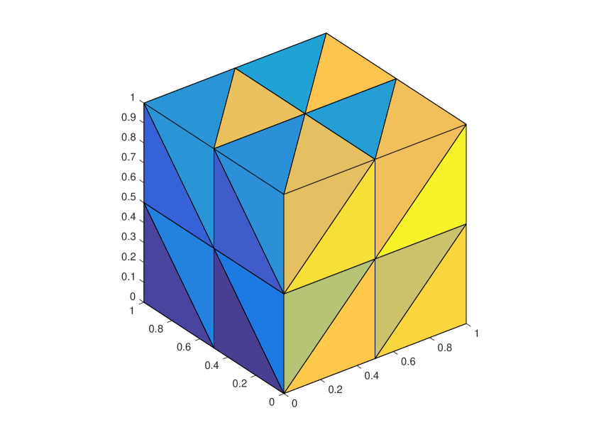
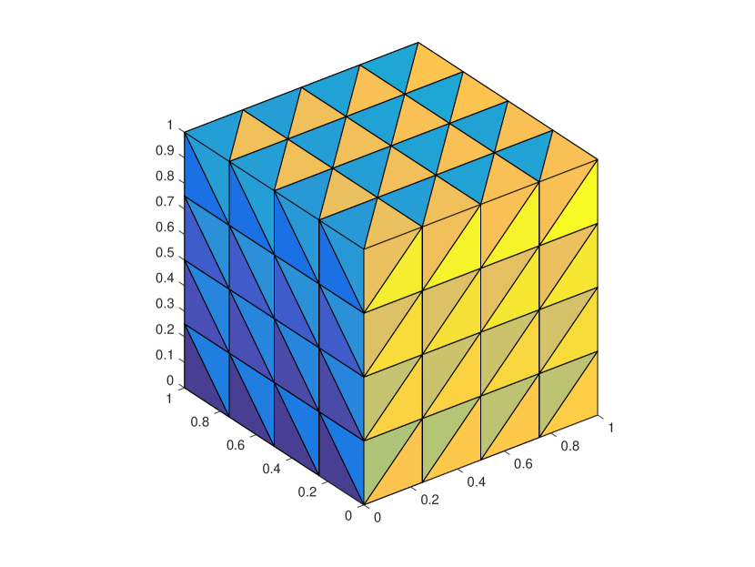
Figure 6.2. Triangulations $\mathcal{T}_{0}$ and $\mathcal{T}_{1}$ for the unit cube

The norms $\|E_{k}\|$ for the error propagation operators of the symmetric $W$-cycle algorithm with $\beta=10^{-2}$ (resp., $\beta=10^{-4}$ and $\beta=10^{-6}$) are displayed in Table 6.6 (resp., Table 6.7 and Table 6.8), where the number $m$ of pre-smoothing and post-smoothing steps increases from $2^{0}$ to $2^{8}$. The times for one iteration of the $W$-cycle algorithm at level 5 (where the number of DOF is roughly $5\times 10^{5}$) are also included.

	1	2	3	4	5	Time
$2^{0}$	3.25e-01	4.12e-01	6.94e-01	8.58e-01	9.04e-01	5.22e-01
$2^{1}$	1.66e-01	2.16e-01	5.27e-01	7.92e-01	8.85e-01	9.33e-01
$2^{2}$	5.06e-02	1.51e-01	3.27e-01	6.69e-01	8.56e-01	1.78e+​00
$2^{3}$	4.83e-03	8.28e-02	1.90e-01	4.92e-01	7.84e-01	3.98e+​00
$2^{4}$	4.41e-05	3.12e-02	1.13e-01	2.89e-01	6.59e-01	6.96e+​00
$2^{5}$	3.68e-09	1.03e-02	5.53e-02	1.71e-01	4.81e-01	1.38e+​01
$2^{6}$	9.23e-17	4.74e-03	2.89e-02	9.65e-02	2.73e-01	2.77e+​01
$2^{7}$	-	2.30e-05	8.31e-03	5.16e-02	1.67e-01	5.48e+​01
$2^{8}$	-	5.28e-10	7.67e-04	2.45e-02	9.64e-02	1.10e+​02

Table 6.6. The norm for the error propagation operator of the symmetric $W$-cycle algorithm with $\beta=10^{-2}$, together with the time (in seconds) for one iteration of the $W$-cycle algorithm at level 5 ($\Omega=$ unit cube)

	1	2	3	4	5	Time
$2^{0}$	1.67e-01	4.90e-01	6.50e-01	7.41e-01	8.58e-01	5.43e-01
$2^{1}$	2.97e-02	2.89e-01	4.74e-01	6.03e-01	8.15e-01	9.37e-01
$2^{2}$	9.87e-04	1.24e-01	2.85e-01	4.20e-01	7.18e-01	1.79e+​00
$2^{3}$	1.07e-06	2.62e-02	1.49e-01	2.48e-01	5.70e-01	4.22e+​00
$2^{4}$	2.53e-10	1.14e-03	5.84e-02	1.49e-01	3.64e-01	7.86e+​00
$2^{5}$	8.22e-17	2.43e-06	1.57e-02	7.39e-02	2.21e-01	1.40e+​01
$2^{6}$	1.36e-18	1.05e-11	7.38e-04	2.27e-02	1.30e-01	2.76e+​01
$2^{7}$	2.31e-17	9.11e-17	1.70e-06	4.88e-03	7.21e-02	5.51e+​01
$2^{8}$	2.10e-17	3.02e-17	9.36e-12	1.66e-04	3.21e-02	1.10e+​02

Table 6.7. The norm for the error propagation operator of the symmetric $W$-cycle algorithm with $\beta=10^{-4}$, together with the time (in seconds) for one iteration of the $W$-cycle algorithm at level 5 ($\Omega=$ unit cube)

	1	2	3	4	5	Time
$2^{0}$	2.52e-01	3.15e-01	7.92e-01	8.96e-01	8.75e-01	5.10e-01
$2^{1}$	6.57e-02	1.26e-01	6.38e-01	8.62e-01	7.94e-01	9.50e-01
$2^{2}$	4.81e-03	1.89e-02	4.25e-01	7.76e-01	6.57e-01	1.78e+​00
$2^{3}$	4.62e-05	1.20e-03	1.96e-01	6.36e-01	4.70e-01	4.04e+​00
$2^{4}$	3.01e-09	1.87e-06	4.15e-02	4.37e-01	2.76e-01	7.75e+​00
$2^{5}$	1.86e-17	3.54e-12	2.19e-03	2.12e-01	1.21e-01	1.38e+​01
$2^{6}$	2.74e-17	3.42e-17	2.47e-05	5.24e-02	3.79e-02	2.77e+​01
$2^{7}$	3.53e-18	7.74e-17	9.88e-10	6.76e-03	7.38e-03	5.55e+​01
$2^{8}$	8.94e-17	1.14e-17	3.25e-16	1.64e-04	1.61e-04	1.10e+​02

Table 6.8. The norm for the error propagation operator of the symmetric $W$-cycle algorithm with $\beta=10^{-6}$, together with the time (in seconds) for one iteration of the $W$-cycle algorithm at level 5 ($\Omega=$ unit cube)

We observe that the symmetric $W$-cycle algorithm is a contraction for $m=1$. The behavior of the contraction numbers agree with Remark 5.6 and they are robust with respect to both $\beta$ and $k$. The performance of the symmetric $V$-cycle algorithm is similar and we only present the numerical results for $m=2^{0}$, $2^{1}$ and $2^{2}$ in Table 6.9.

	1	2	3	4	5	Time
$\beta=10^{-2}$
$2^{0}$	3.25e-01	4.45e-01	6.46e-01	7.99e-01	8.55e-01	4.27e-01
$2^{1}$	1.66e-01	2.77e-01	4.87e-01	7.49e-01	8.47e-01	7.72e-01
$2^{2}$	5.06e-02	1.69e-01	2.95e-01	6.40e-01	8.17e-01	1.49e+​00
$\beta=10^{-4}$
$2^{0}$	1.67e-01	4.88e-01	6.44e-01	7.37e-01	8.18e-01	4.25e-01
$2^{1}$	2.97e-02	2.89e-01	4.65e-01	6.00e-01	7.62e-01	8.07e-01
$2^{2}$	9.87e-04	1.24e-01	2.78e-01	4.20e-01	6.71e-01	1.49e+​00
$\beta=10^{-6}$
$2^{0}$	2.52e-01	3.13e-01	7.92e-01	8.88e-01	8.86e-01	4.39e-01
$2^{1}$	6.57e-02	1.26e-01	6.38e-01	8.47e-01	8.19e-01	7.87e-01
$2^{2}$	4.81e-03	1.89e-02	4.25e-01	7.70e-01	7.05e-01	1.66e+​00

Table 6.9. The norm for the error propagation operator of the symmetric $V$-cycle algorithm, together with the time (in seconds) for one iteration of the $V$-cycle algorithm at level 5 ($\Omega=$ unit cube)

7. Concluding Remarks

In this paper we construct multigrid algorithms for a model linear-quadratic elliptic optimal control problem and prove that for convex domains the $W$-cycle algorithm with a sufficiently large number of smoothing steps is uniformly convergent with respect to mesh refinements and a regularizing parameter. The theoretical estimates and the performance of the algorithms are demonstrated by numerical results.

For the numerical results in Section 6, we use a $V(4,4)$ multigrid solve for (3.11) in the construction of the preconditioner $\mathfrak{C}_{k}^{-1}$. But in fact the symmetric $V$-cycle multigrid algorithm from Section 3.4 based on a $V(1,1)$ solve for (3.11) also converges uniformly with $1$ pre-smoothing step and $1$ post-smoothing step. The results for the unit square and unit cube are reported in Table 7.1 and Table 7.2.

	1	2	3	4	5	6	7	Time
$10^{-2}$	2.15e-01	7.92e-01	8.20e-01	8.24e-01	8.29e-01	8.33e-01	8.36e-01	4.99e-02
$10^{-4}$	6.32e-02	2.83e-01	6.25e-01	8.11e-01	8.23e-01	8.30e-01	8.35e-01	4.59e-02
$10^{-6}$	2.56e-01	6.49e-01	7.22e-01	8.36e-01	9.52e-01	9.56e-01	9.58e-01	4.58e-02

Table 7.1. The norm for the error propagation operator of the symmetric $V$-cycle algorithm from Section 3.4 with $m=1$, together with the time (in seconds) for one iteration of the $V$-cycle algorithm at level 7 ($\Omega=$ unit square)

	1	2	3	4	5	Time
$10^{-2}$	3.91e-01	6.63e-01	8.16e-01	8.71e-01	8.92e-01	3.21e-01
$10^{-4}$	1.72e-01	7.17e-01	8.42e-01	8.84e-01	9.05e-01	3.18e-01
$10^{-6}$	2.70e-01	5.76e-01	9.31e-01	9.47e-01	9.47e-01	3.15e-01

Table 7.2. The norm for the error propagation operator of the symmetric $V$-cycle algorithm from Section 3.4 with $m=1$, together with the time (in seconds) for one iteration of the $V$-cycle algorithm at level 5 ($\Omega=$ unit cube)

Moreover numerical results indicate that our multigrid algorithms are also robust for nonconvex domains. The results for the symmetric $V$-cycle algorithm with 1 pre-smoothing step and 1 post-smoothing step can be found in Table 7.3, where the preconditioner is also based on a $V(1,1)$ solve for (3.11). (The number of DOF at level 6 is roughly $4.8\times 10^{4}$.) However our theory for the convex domain does not immediately generalize to nonconvex domains. Note that nonconvex domains have been treated in [21] with respect to an abstract norm defined through the interpolation between function spaces.

	1	2	3	4	5	6	Time
$10^{-2}$	8.36e-01	8.19e-01	8.21e-01	8.36e-01	8.59e-01	8.89e-01	3.81e-02
$10^{-4}$	1.86e-01	3.54e-01	6.81e-01	7.17e-01	7.25e-01	7.29e-01	3.84e-02
$10^{-6}$	4.74e-01	5.07e-01	7.07e-01	8.67e-01	8.91e-01	9.07e-01	3.82e-02

Table 7.3. The norm for the error propagation operator of the symmetric $V$-cycle algorithm from Section 3.4 with $m=1$, together with the time (in seconds) for one iteration of the $V$-cycle algorithm at level 7 ($\Omega=$ $L$-shaped domain)

One of the features of our multigrid algorithms is that they can be applied to nonsymmetric saddle point problems with only a trivial modification (cf. [6, 7]). For example, we can also modify our multigrid algorithms to solve an optimal control problem with the constraint (1.2) replaced by

$$(\nabla y,\nabla v)_{L_{2}(\Omega)}+(\bm{\zeta}\cdot\nabla y,v)_{L_{2}(\Omega)}=(u,v)_{L_{2}(\Omega)}\qquad\forall\,v\in H^{1}_{0}(\Omega),$$

where $\bm{\zeta}\in[W^{1,\infty}(\Omega)]^{d}$ and $\nabla\cdot\bm{\zeta}=0$. This and the extension of our theory to nonconvex domains and the $V$-cycle algorithm will be investigated in our ongoing projects.

References

- [1] I. Babuška. The finite element method with Lagrange multipliers. Numer. Math., 20:179–192, 1973.
- [2] A. Borzì and V. Schulz. Multigrid methods for PDE optimization. SIAM Rev., 51:361–395, 2009.
- [3] A. Borzì and V. Schulz. Computational Optimization of Systems Governed by Partial Differential Equations. Society for Industrial and Applied Mathematics, Philadelphia, PA, 2012.
- [4] J.H. Bramble and X. Zhang. The Analysis of Multigrid Methods. In P.G. Ciarlet and J.L. Lions, editors, Handbook of Numerical Analysis, VII, pages 173–415. North-Holland, Amsterdam, 2000.
- [5] S.C. Brenner, H. Li, and L.-Y. Sung. Multigrid methods for saddle point problems: Stokes and Lamé systems. Numer. Math., 128:193–216, 2014.
- [6] S.C. Brenner, H. Li, and L.-Y. Sung. Multigrid methods for saddle point problems: Oseen system. Comput. Math. Appl., 74:2056–2067, 2017.
- [7] S.C. Brenner, D.-S. Oh, and L.-Y. Sung. Multigrid methods for saddle point problems: Darcy systems. Numer. Math., 138:437–471, 2018.
- [8] S.C. Brenner and L.R. Scott. The Mathematical Theory of Finite Element Methods Third Edition. Springer-Verlag, New York, 2008.
- [9] F. Brezzi. On the existence, uniqueness and approximation of saddle-point problems arising from Lagrangian multipliers. RAIRO Anal. Numér., 8:129–151, 1974.
- [10] P.G. Ciarlet. The Finite Element Method for Elliptic Problems. North-Holland, Amsterdam, 1978.
- [11] M. Dauge. Elliptic Boundary Value Problems on Corner Domains, Lecture Notes in Mathematics 1341. Springer-Verlag, Berlin-Heidelberg, 1988.
- [12] H.C. Elman, D.J. Silvester, and A.J. Wathen. Finite Elements and Fast Iterative Solvers: with Applications in Incompressible Fluid Dynamics. Oxford University Press, Oxford, second edition, 2014.
- [13] M. Engel and M. Griebel. A multigrid method for constrained optimal control problems. J. Comput. Appl. Math., 235:4368–4388, 2011.
- [14] P. Grisvard. Elliptic Problems in Non Smooth Domains. Pitman, Boston, 1985.
- [15] W. Hackbusch. Multi-grid Methods and Applications. Springer-Verlag, Berlin-Heidelberg-New York-Tokyo, 1985.
- [16] J.-L. Lions. Optimal Control of Systems Governed by Partial Differential Equations. Springer-Verlag, New York, 1971.
- [17] J. Mandel, S. McCormick, and R. Bank. Variational Multigrid Theory. In S. McCormick, editor, Multigrid Methods, Frontiers In Applied Mathematics 3, pages 131–177. SIAM, Philadelphia, 1987.
- [18] K.-A. Mardal and R. Winther. Preconditioning discretizations of systems of partial differential equations. Numer. Linear Algebra Appl., 18:1–40, 2011.
- [19] Y. Saad. Iterative Methods for Sparse Linear Systems. SIAM, Philadelphia, 2003.
- [20] J. Schöberl, R. Simon, and W. Zulehner. A robust multigrid method for elliptic optimal control problems. SIAM J. Numer. Anal., 49:1482–1503, 2011.
- [21] S. Takacs and W. Zulehner. Convergence analysis of all-at-once multigrid methods for elliptic control problems under partial elliptic regularity. SIAM J. Numer. Anal., 51:1853–1874, 2013.
- [22] F. Tröltzsch. Optimal Control of Partial Differential Equations. American Mathematical Society, Providence, RI, 2010.
- [23] S.W. Walker. FELICITY: A MATLAB/C++ toolbox for developing finite element methods and simulation modeling. SIAM J. Sci. Comput., 40:C234–C257, 2018.
- [24] J. Xu and L. Zikatanov. Some observations on Babuška and Brezzi theories. Numer. Math., 94:195–202, 2003.