3D MHD modeling of the expanding remnant of SN 1987A

Abstract

Aims. We investigate the role played by a pre-supernova (SN) ambient magnetic field on the dynamics of the expanding remnant of SN 1987A and the origin and evolution of the radio emission from the remnant, in particular, during the interaction of the blast wave with the nebula surrounding the SN.

Methods. We model the evolution of SN 1987A from the breakout of the shock wave at the stellar surface to the expansion of its remnant through the surrounding nebula by three-dimensional magnetohydrodynamic simulations. The model considers the radiative cooling, the deviations from equilibrium of ionization, the deviation from temperature-equilibration between electrons and ions, and a plausible configuration of the pre-SN ambient magnetic field. We explore strengths of the pre-SN magnetic field ranging between $1\mu$G and $100\mu$G at the inner edge of the nebula and we assume an average field strength at the stellar surface $B_{0}\approx 3$ kG. From the simulations, we synthesize both thermal X-ray and non-thermal radio emission and compare the model results with observations.

Results. The presence of an ambient magnetic field with strength in the range considered does not change significantly the overall evolution of the remnant. Nevertheless, the magnetic field reduces the erosion and fragmentation of the dense equatorial ring after the impact of the SN blast wave. As a result, the ring survives the passage of the blast, at least, during the time covered by the simulations (40 years). Our model is able to reproduce the morphology and lightcurves of SN 1987A in both X-ray and radio bands. The model reproduces the observed radio emission if the flux originating from the reverse shock is heavily suppressed. In this case, the radio emission originates mostly from the forward shock traveling through the H II region and this may explain why the radio emission seems to be insensitive to the interaction of the blast with the ring. Possible mechanisms for the suppression of emission from the reverse shock are investigated. We find that synchrotron self-absorption and free-free absorption have negligible effects on the emission during the interaction with the nebula. We suggest that the emission from the reverse shock at radio frequencies might be limited by highly magnetized ejecta.

1 Introduction

The expanding remnant of SN 1987A in the Large Magellanic Cloud offers the opportunity to study in great detail the transition from the phase of supernova (SN) to that of supernova remnant (SNR), thanks to its youth (the SN was observed on 1987 February 23; West et al. 1987) and proximity (at about 51.4 kpc from Earth; Panagia 1999). SN 1987A has been the subject of an intensive international observing campaign, incorporating observations at every possible wavelength. The SN explosion and the subsequent evolution of its remnant have been monitored continuously since the collapse of the progenitor star, Sanduleak (Sk) $−69^{\rm o}202$, a blue supergiant (BSG) with an initial mass of $\approx 20\,M_{\odot}$ (Hillebrandt et al. 1987).

Observations in different wavelength bands have revealed that the pre-SN circumstellar medium (CSM) around SN 1987A is highly inhomogeneous (e.g. Crotts et al. 1989; Sugerman et al. 2005). It is characterized by an extended nebula consisting mainly of three dense rings, one lying in the equatorial plane, and two less dense ones lying in planes almost parallel to the equatorial one, but displaced by about 0.4 pc above and below the central ring; the rings are immersed in a much larger and tenuous H II region with peanut-shaped structure with a maximum extension of about 6 pc in the direction perpendicular to the equatorial plane. General consensus is that the stellar progenitor went, first, through a phase of red supergiant (RSG) and, then, through that of BSG before the collapse (Crotts & Heathcote 2000). The nebula resulted from the interaction between the fast wind emitted during the phase of BSG and the relic denser and slower wind emitted previously during the phase of RSG (e.g. Chevalier & Dwarkadas 1995; Morris & Podsiadlowski 2007; Chita et al. 2008).

Radio and X-ray observations collected in the last $\approx 30$ years have monitored in detail the interaction of the SN blast wave with the nebula (for a comprehensive review see McCray & Fransson 2016). The interaction started about 3 years after the explosion, when both radio and X-ray fluxes have suddenly increased (e.g. Hasinger et al. 1996; Gaensler et al. 1997). This was interpreted as being due to the blast wave impacting onto the H II region and starting to travel in a medium much denser than that of the BSG wind. In the subsequent years the radio and X-ray fluxes have continued to rise together. After about 14 years, however, the soft X-ray light curve has steepened still further, contrary to the hard X-ray and radio lightcurves (Park et al. 2005) which continued to increase with almost constant slope. This has indicated a source of emission that leads predominantly to soft X-rays and was interpreted as being due to the blast wave sweeping up the dense central equatorial ring (McCray 2007). Since then the soft X-ray lightcurve has continued to increase indicating that the blast wave was traveling through the dense ring (Helder et al. 2013). In its latest X-ray observations, Chandra has recorded a significant change in the soft X-ray lightcurve which has remained constant since year 26 (Frank et al. 2016). This has been interpreted as being due to the blast wave leaving the ring and starting to travel in a less dense environment. A similar conclusion has been obtained more recently in the radio band from the analysis of observations taken with the Australia Telescope Compact Array (ATCA; Cendes et al. 2018).

The evolution and morphology of the radio emission from SN 1987A have been investigated by Potter et al. (2014) through a three-dimensional (3D) hydrodynamic (HD) model describing the interaction of the SN blast wave with the nebula between years 2 and 27. Their best-fit model is able to reproduce the evolution of the radio emission reasonably well, although it predicts a significant steepening of radio flux when the blast wave hits the central ring, at odds with observations. As for the evolution of the X-ray emission, Orlando et al. (2015) have proposed a 3D HD model which describes the evolution of SN 1987A since the shock breakout at the stellar surface (few hours after the core-collapse), and which covers 40 years of evolution. Their best-fit model is able to reproduce quite well, at the same time, the bolometric lightcurve of the SN observed during the first 250 days of evolution, and the X-ray emission (morphology, lightcurves, and spectra) of the subsequent expanding remnant (see also Miceli et al. 2018, submitted to Nature Astronomy).

Current models of SN 1987A, however, do not include the effects of an ambient magnetic field. The latter is expected to not affect significantly the overall evolution (and the morphology) of the remnant. Nevertheless it may play a role during the interaction of the blast wave with the ring by dumping the HD instabilities (responsible for the fragmentation of the ring) that would develop during the interaction (e.g. Orlando et al. 2008). Also, modeling the magnetic field is necessary to synthesize self-consistently from the models the non-thermal radio emission. In the model of Potter et al. (2014) the magnetic field is not modeled but the radio emission is synthesized by assuming a randomly oriented magnetic field at the shock front, using analytic estimates for cosmic-ray (CR) driven magnetic field amplification. Also, it is not clear from the literature where the radio emission originates and why the radio flux seems to be insensitive to the interaction of the blast wave with the dense ring.

Here we investigate the role played by an ambient magnetic field on the evolution of the remnant and, more specifically, during the interaction of the SN blast wave with the nebula. Also, we aim at exploring the origin of non-thermal radio emission from SN 1987A and possible diagnostics of the inhomogeneous CSM in which the explosion occurred. To this end, we model the evolution of SN 1987A using detailed 3D MHD simulations. From the simulations we synthesize the thermal X-ray and non-thermal radio emission (including the modeling of the post-shock evolution of relativistic electrons and the observed evolution of the radio spectral index) and compare the synthetic lightcurves with those inferred from the analysis of observations.

In Sect. 2 we describe the MHD model, the numerical setup, and the synthesis of thermal X-ray and non-thermal radio emission; in Sect. 3 we discuss the results; and finally in Sect. 4 we draw our conclusions.

2 MHD modeling

The model describes the evolution of SN 1987A from the breakout of the shock wave at the stellar surface (occurring few hours after the SN event) to the interaction of the blast wave and ejecta caused by the explosion with the surrounding nebula. The model covers 40 years of evolution to provide also some hints on the evolution of the expanding remnant expected in the near future, namely when the Square Kilometer Array (SKA) in radio and the Athena satellite in X-rays will be in operation. The computational strategy is the same as described in Orlando et al. (2015) and consists of two steps (see also Orlando et al. 2016): first, we modeled the “early” post-explosion evolution of a CC-SN during the first 24 hours through 1D simulations; then, we mapped the output of these simulations into 3D and modeled the transition from the phase of SN to that of SNR and the interaction of the remnant with the inhomogeneous pre-SN environment (see Orlando et al. 2015 for further details).

In this work, for the post-explosion evolution of the SN during the first 24 hours, we adopted the best-fit model (model SN-M17-E1.2-N8) described in Orlando et al. (2015) (see their Table 3); the model is characterized by an explosion energy of $1.2\times 10^{51}$ erg and an envelope mass of 17 $M_{\odot}$. The SN evolution has been simulated by a 1D Lagrangian code in spherical geometry which solves the equations of relativistic radiation hydrodynamics, for a self-gravitating matter fluid interacting with radiation (Pumo & Zampieri 2011). The code is fully general relativistic and provides an accurate treatment of radiative transfer at all regimes (from the one in which the ejecta are optically thick up to when they are optically thin).

This 1D simulation of the SN provides the radial distribution of ejecta (density, pressure, and velocity) about 24 hours after the SN event. Then we mapped the 1D profiles in the 3D domain and started 3D MHD simulations which describe the interaction of the remnant with the surrounding nebula. The evolution of the blast wave was modeled by numerically solving the full time-dependent MHD equations in a 3D Cartesian coordinate system $(x,y,z)$, including the effects of the radiative losses from optically thin plasma. The MHD equations were solved in the non-dimensional conservative form:

$$\frac{\partial\rho}{\partial t}+\nabla\cdot(\rho\@vec{u})=0\leavevmode\nobreak\ ,$$ (1)

$$\frac{\partial\rho\@vec{u}}{\partial t}+\nabla\cdot(\rho\@vec{u}\@vec{u}-\@vec{B}\@vec{B})+\nabla P_{*}=0\leavevmode\nobreak\ ,$$ (2)

$$\frac{\partial\rho E}{\partial t}+\nabla\cdot[\@vec{u}(\rho E+P_{*})-\@vec{B}(\@vec{u}\cdot\@vec{B})]=-n_{\rm e}n_{\rm H}\Lambda(T)\leavevmode\nobreak\ ,$$ (3)

$$\frac{\partial\@vec{B}}{\partial t}+\nabla\cdot(\@vec{u}\@vec{B}-\@vec{B}\@vec{u})=0\leavevmode\nobreak\ ,$$ (4)

where

$$P_{*}=P+\frac{B^{2}}{2}\leavevmode\nobreak\ ,\leavevmode\nobreak\ \leavevmode\nobreak\ \leavevmode\nobreak\ \leavevmode\nobreak\ \leavevmode\nobreak\ \leavevmode\nobreak\ \leavevmode\nobreak\ \leavevmode\nobreak\ \leavevmode\nobreak\ \leavevmode\nobreak\ \leavevmode\nobreak\ \leavevmode\nobreak\ \leavevmode\nobreak\ E=\epsilon+\frac{1}{2}u^{2}+\frac{1}{2}\frac{B^{2}}{\rho}\leavevmode\nobreak\ ,$$

are the total pressure, and the total gas energy (internal energy, $\epsilon$, kinetic energy, and magnetic energy) respectively, $t$ is the time, $\rho=\mu m_{H}n_{\rm H}$ is the mass density, $\mu$ is the mean atomic mass, $m_{H}$ is the mass of the hydrogen atom, $n_{\rm H}$ is the hydrogen number density, $\@vec{u}$ is the gas velocity, $T$ is the temperature, $\@vec{B}$ is the magnetic field, and $\Lambda(T)$ represents the optically thin radiative losses per unit emission measure derived with the PINTofALE spectral code (Kashyap & Drake, 2000) with the APED V1.3 atomic line database (Smith et al., 2001), assuming metal abundances appropriate for SN 1987A (Zhekov et al. 2009). We used the ideal gas law, $P=(\gamma-1)\rho\epsilon$, where $\gamma=5/3$ is the adiabatic index.

The simulations of the expanding SNR were performed using pluto (Mignone et al., 2007, 2012), a modular Godunov-type code intended mainly for astrophysical applications and high Mach number flows in multiple spatial dimensions. The code is designed to make efficient use of massively parallel computers using the message-passing interface (MPI) for interprocessor communications. The MHD equations are solved using the MHD module available in pluto, configured to compute intercell fluxes with the Harten-Lax-van Leer discontinuities (HLLD) approximate Riemann solver, while third order in time is achieved using a Runge-Kutta scheme. Miyoshi & Kusano (2005) have shown that the HLLD algorithm is very efficient in solving discontinuities formed in the MHD system; consequently the adopted scheme is particularly appropriate to describe the shocks formed during the interaction of the remnant with the surrounding inhomogeneous medium. A monotonized central difference limiter (the least diffusive limiter available in pluto) for the primitive variables is used. The solenoidal constraint of the magnetic field is controlled by adopting an hyperbolic/parabolic divergence cleaning technique available in pluto (Dedner et al. 2002; Mignone et al. 2010). The optically thin radiative losses are included in a fractional step formalism (Mignone et al., 2007); in such a way, the $2^{nd}$ time accuracy is preserved as the advection and source steps are at least of the $2^{nd}$ order accurate. The radiative losses $\Lambda$ values are computed at the temperature of interest using a table lookup/interpolation method. The code was extended by additional computational modules to calculate the deviations from temperature-equilibration between electrons and ions (by including the almost instantaneous heating of electrons at shock fronts up to $kT\leavevmode\nobreak\ 0.3$ keV by lower hybrid waves - Ghavamian et al. 2007 - and the effects of Coulomb collisions for the calculation of ion and electron temperatures in the post-shock plasma; see Orlando et al. 2015 for further details) and the deviations from equilibrium of ionization of the most abundant ions (through the computation of the maximum ionization age in each cell of the spatial domain; Orlando et al. 2015).

Following Orlando et al. (2015), we assumed that the initial (about 24 hours after the SN event) density structure of the ejecta was clumpy, as also suggested by both theoretical studies (e.g. Nagataki 2000; Kifonidis et al. 2006; Wang & Wheeler 2008; Gawryszczak et al. 2010; Wongwathanarat et al. 2015) and spectropolarimetric studies of SNe (e.g. Wang et al. 2003, 2004; Hole et al. 2010). Therefore, after the 1D radial density distribution of ejecta (from model SN-M17-E1.2-N8; see above) was mapped into 3D, the small-scale clumping of material is modeled as per-cell random density perturbations derived from a power-law probability distribution (Orlando et al. 2012, 2015). In our simulations, we considered ejecta clumps with the same initial size $2\times 10^{12}$ cm (corresponding to $\approx 1$% of the initial remnant radius), and a maximum density perturbation $\nu_{\rm max}=5$.

The CSM around SN 1987A is modeled as in Orlando et al. (2015). In particular, we considered a spherically symmetric wind in the immediate surrounding of the SN event which is characterized by a gas density proportional to $r^{-2}$ (where $r$ is the radial distance from the center of explosion), a mass-loss rate of $\dot{M}_{\rm w}=10^{-7}M_{\odot}$ year^-1, and a wind velocity $u_{\rm w}=500$ km s^-1 (see also Morris & Podsiadlowski 2007); the termination shock of the wind is located approximately at $r_{\rm w}=0.05$ pc. The circumstellar nebula was modeled assuming that it consists of an extended ionized H II region and a dense inhomogeneous equatorial ring (see Fig. 1 in Orlando et al. 2015) composed by a uniform smooth component and high-density spherical clumps mostly located in its inner portion (e.g. Chevalier & Dwarkadas 1995; Sugerman et al. 2005). The H II region has density $n_{\rm HII}$ and its inner edge in the equatorial plane is at distance $r_{\rm HII}$ from the center of explosion. The uniform smooth component of the ring has density $n_{\rm rg}$, radius $r_{\rm rg}$, and an elliptical cross section with the major axis $w_{\rm rg}$ lying on the equatorial plane and height $h_{\rm rg}$; the $N_{\rm cl}$ clumps have a diameter $w_{\rm cl}$ and their plasma density and radial distance from SN 1987A are randomly distributed around the values $<n_{\rm cl}>$ and $<r_{\rm cl}>$ respectively. In this paper we adopted the parameters of the CSM derived in Orlando et al. (2015) to reproduce the X-ray observations (namely the morphology, lightcurves and spectra) of SN 1987A during the first $\approx 30$ years of evolution. Table 1 summarizes the parameters adopted.

Table 1: Adopted parameters of the CSM for the MHD model of SN 1987A.

CSM component	Parameters	Units	Best-fit values
BSG wind:	$\dot{M}_{\rm w}$	($M_{\odot}$ year-1)	$10^{-7}$
	$u_{\rm w}$	(km s-1)	500
	$r_{\rm w}$	(pc)	0.05
H II region:	$n_{\rm HII}$	($10^{2}$ cm-3)	0.9
	$r_{\rm HII}$	(pc)	0.08
Equatorial ring:	$n_{\rm rg}$	($10^{3}$ cm-3)	1
	$r_{\rm rg}$	(pc)	0.18
	$w_{\rm rg}$	($10^{17}$ cm)	$1.7$
	$h_{\rm rg}$	($10^{16}$ cm)	$3.5$
Clumps:	$<n_{\rm cl}>$	($10^{4}$ cm-3)	$2.5\pm 0.3$
	$<r_{\rm cl}>$	(pc)	$0.155\pm 0.015$
	$w_{\rm cl}$	($10^{16}$ cm)	$1.7$
	$N_{\rm cl}$		50

The simulations include passive tracers to follow the evolution of the different plasma components (ejecta, H II region, and ring material) and to store information on the shocked plasma (time, shock velocity, and shock position, i.e. Lagrangian coordinates, when a cell of the mesh is shocked either by the forward or by the reverse shock) required to synthesize the thermal X-ray and non-thermal radio emission (see Sects. 2.2 and 2.3). The continuity equations of the tracers are solved in addition to our set of MHD equations. In the case of tracers associated with the different plasma components, each material is initialized with $C_{\rm i}=1$, while $C_{\rm i}=0$ elsewhere, where the index “i” refers to the ejecta (ej), the H II region (HII), and the ring material (rg). All the other tracers are initialized to zero everywhere.

The initial computational domain is a Cartesian box extending between $-4\times 10^{14}$ cm and $4\times 10^{14}$ cm in the $x$, $y$, and $z$ directions. The box is covered by a uniform grid of $1024^{3}$ zones, leading to a spatial resolution of $\approx 8\times 10^{11}$ cm ($\approx 2.6\times 10^{-7}$ pc). The SN explosion is assumed to sit at the origin of the 3D Cartesian coordinate system $(x_{0},y_{0},z_{0})=(0,0,0)$. In order to follow the large physical scales spanned during the remnant expansion, we followed the same mesh strategy as proposed by Ono et al. (2013) in the modeling of core-collapse SN explosions (see also Nagataki et al. 1997). More specifically, the computational domain was gradually extended as the forward shock propagates and the physical values were remapped in the new domains. When the forward shock is close to one of the boundaries of the Cartesian box, the physical size of the computational domain is extended by a factor of 1.2 in all directions, maintaining a uniform grid of $1024^{3}$ zones. All the physical quantities in the extended region are set to the values of the pre-SN CSM. As discussed by Ono et al. (2013), this approach is possible because the propagation of the forward shock is supersonic and it does not introduce errors larger than 0.1% after 40 re-mappings. We found that 43 re-mappings were necessary to follow the interaction of the blast wave with the CSM during 40 years of evolution. The final domain extends between $-10^{18}$ cm and $10^{18}$ cm in the $x$, $y$, and $z$ directions, leading to a spatial resolution of $\approx 2\times 10^{15}$ cm ($\approx 6.5\times 10^{-4}$ pc). This strategy guaranteed to have more than 400 zones per remnant radius during the whole evolution. All physical quantities were set to the values of the pre-SN CSM at all boundaries.

2.1 Pre-supernova ambient magnetic field

Our simulations include the effect of an ambient magnetic field. This field is not expected to influence the overall expansion and evolution of the blast wave which is characterized by a high plasma $\beta$ (defined as the ratio between thermal pressure and magnetic pressure). Nevertheless, a magnetic field is required for the synthesis of radio emission (see Sect. 2.3) and it might play a role locally in preserving inhomogeneities of the CSM (as the equatorial ring and the clumps) from complete fragmentation (by limiting the growth of HD instabilities; e.g. Orlando et al. 2008). For these reasons, we introduced a seed magnetic field in our simulations.

The characteristics of magnetic fields around massive stars, and the way these fields, in combination with stellar rotation, confine stellar wind outflows of massive stars (thus building up an extended circumstellar magnetosphere) have been studied in the literature through accurate MHD simulations (e.g. Townsend & Owocki 2005; Townsend et al. 2005; ud-Doula et al. 2008, 2013). However, at present, there is no hint about the initial magnetic field strength and configuration around Sk $−69^{\rm o}202$ which resulted from the merging of two massive stars. Therefore we assumed here the simplest and most common magnetic field configuration around a rotating star.

Most likely, the ambient magnetic field is that originating from the stellar progenitor. Petermann et al. (2015) have argued that BSGs descend from magnetic massive stars. These stars can result from strong binary interaction and, in particular, from the merging of two main sequence stars (Sana et al. 2012), as it is the case for Sk $−69^{\rm o}202$ (e.g. Morris & Podsiadlowski 2007). In magnetic massive stars, the observed fields are, in general, large scale fields with a dominant dipole component and with typical values at the stellar surface varying in the range between 100 G and 10 kG (see the review by Donati & Landstreet 2009). Due to the rotation of the progenitor and to the expanding stellar wind, the field is expected to be twisted around the rotation axis of the progenitor, even if magnetic massive stars generally rotate more slowly than normal stars of the same mass, by factors of ten to 1000 (e.g. Donati & Landstreet 2009). Thus we expect that the field might be characterized by a toroidal component resulting in the so-called “Parker spiral”, in analogy with the spiral-shaped magnetic field on the interplanetary medium of the solar system (Parker 1958). For the purposes of the present paper, we assumed as initial ambient magnetic field, a Parker spiral which, in spherical coordinates $(r,\theta,\phi)$, can be described by the radial and toroidal components:

$$B_{\rm r}=\frac{A_{1}}{r^{2}}\leavevmode\nobreak\ ,\leavevmode\nobreak\ \leavevmode\nobreak\ \leavevmode\nobreak\ \leavevmode\nobreak\ \leavevmode\nobreak\ \leavevmode\nobreak\ \leavevmode\nobreak\ \leavevmode\nobreak\ B_{\phi}=-\frac{A_{2}}{r}\sin\theta$$ (5)

where

$$A_{1}=B_{0}r_{0}^{2}\leavevmode\nobreak\ ,\leavevmode\nobreak\ \leavevmode\nobreak\ \leavevmode\nobreak\ \leavevmode\nobreak\ \leavevmode\nobreak\ \leavevmode\nobreak\ \leavevmode\nobreak\ \leavevmode\nobreak\ A_{2}=B_{0}r_{0}^{2}\omega_{\rm s}/u_{\rm w}\leavevmode\nobreak\ ,$$ (6)

$B_{0}$ is the average magnetic field strength at the stellar surface, $r_{0}$ the stellar radius, $\omega_{\rm s}$ the angular velocity of stellar rotation, and $u_{\rm w}$ the wind speed. In the case of SN 1987A, the field configuration probably resulted from the different phases in the evolution of the stellar progenitor whose details are poorly known; thus the field configuration can be more complex than that described here. Recently, Zanardo et al. (2018) have estimated the strength of the ambient (pre-shock) magnetic field within the nebula $\approx 30\,\mu$G and the (post-shock) field strength within the remnant of the order of a few mG. In the light of this, we considered two cases in which the field strength is almost the same in proximity of the initial remnant ($t\approx 24$ hours), whereas it is either of the order of $1\,\mu$G (run MOD-B1) or of the order of $100\,\mu$G (run MOD-B100) at the inner edge of the nebula (at a distance from the center of explosion $r\approx 0.08$ pc). This is realized by considering the parameter $A_{1}=3\times 10^{28}$ G cm² in both cases, and $A_{2}=8\times 10^{10}$ G cm in MOD-B1 and $A_{2}=8\times 10^{13}$ G cm in MOD-B100. If $r_{0}\approx 45\,R_{\odot}$ is the radius of the BSG progenitor of SN 1987A (Woosley 1988), from Eq. 6 $B_{0}\approx 3$ kG in both models, a value well within the range inferred for magnetic massive stars (e.g. Donati & Landstreet 2009).

As expected, the adopted field strength does not influence significantly the evolution of the remnant, being the plasma $\beta>10^{5}$ at the forward shock after the breakout of the shock wave at the stellar surface. By comparing the SNR ram pressure, thermal pressure, and ambient magnetic field pressure soon after the shock breakout, we note that the remnant expansion and dynamics could have been significantly affected by the ambient magnetic field if its strength close to the stellar surface had been larger than 1 MG, a value much higher than the typical field strengths observed in massive stars (e.g. Donati & Landstreet 2009).

Finally, it is worth noting that our Eqs. 5-6 describe the magnetic field also in the initial ($t\approx 24$ hours) remnant interior. We expect, however, that a more realistic field there (especially in the immediate surroundings of the remnant compact object) would be much more complex than that adopted here and it should reflect the field of the stellar interior before the collapse of the stellar progenitor. Current stellar evolution models predict that differentially rotating massive stars have relatively weak fields before collapse (e.g. Heger et al. 2005). Nevertheless several mechanisms for efficient field amplification after core bounce may be present (e.g. Obergaulinger et al. 2014; Masada et al. 2018, for non-rotating progenitors; Obergaulinger & Aloy 2017, for rotating models). Among these, magneto-rotational instability (MRI) driven by the combined action of magnetic field and rotation may produce dynamically relevant fields after bounce which can affect the evolution of the SN (e.g. Masada et al. 2012; Rembiasz et al. 2016a, b). In the case of a star with mass similar to that presumed for Sk $−69^{\rm o}202$ ($\approx 20M_{\odot}$), Obergaulinger et al. (2018) have explored the effects of magnetic field and rotation on the core collapse by considering different, artificially added profiles of rotation and magnetic field. They found that the evolution of the shock wave can be modified if the field is in equipartition with the gas pressure: the explosion geometry is bipolar with two outflows propagating along the rotational axis and downflows at low latitudes. The strength of the magnetic field (in combination with rotation) therefore can have significant effects on the evolution of the SN. In the case of SN 1987A, however, we do not have any indication about the strength and configuration of the stellar magnetic field during the core-collapse and the expansion of the shock wave through the stellar interior. Thus, for the sake of simplicity, we assumed here that the field is weak enough that the magnetic energy density is much lower than the kinetic energy of ejecta or, in other words, that the field has no significant influence on the ejecta dynamics.

Figure 1 shows the initial configuration of the ambient magnetic field in models MOD-B1 and MOD-B100. In the latter model, the toroidal component of the magnetic field is largely dominant.

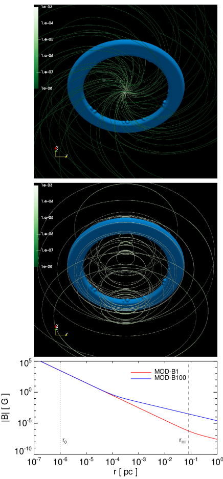
Figure 1: Initial configuration of the pre-SN ambient magnetic field for models MOD-B1 (upper panel) and MOD-B100 (middle panel). The green lines are sampled magnetic field lines; the scale of the magnetic field strength is log and is given by the bar on the left of each panel, in units of $G$. The unshocked equatorial ring material (with $n\geq 1000$ cm^-3) is marked blue; the figure does not show the H II region around the ring. The lower panel shows the radial magnetic field strength in the equatorial plane for the two models; the dotted line marks the radius of the BSG progenitor, the dashed line marks the inner edge of the H II region.

2.2 Synthesis of thermal X-ray emission

We followed the approach outlined in Orlando et al. (2015) to synthesize, from the model results, the thermal X-ray emission originating from the impact of the blast wave with the nebula. In this section, we summarize the main steps in this approach; we refer the reader to Sect. 2.3 in Orlando et al. (2015) for more details (see also Orlando et al. 2006, 2009).

As a first step, we rotated the system about the three axis to fit the orientation of the ring with respect to the line-of-sight (LoS) as found from the analysis of optical data (Sugerman et al. 2005): $i_{x}=41^{\rm o}$, $i_{y}=-8^{\rm o}$, and $i_{z}=-9^{\rm o}$. Then, for each $j$th cell of the spatial domain, we derived: a) the emission measure as em${}_{\rm j}=n_{\rm Hj}^{2}V_{\rm j}$ (where $n_{\rm Hj}^{2}$ is the hydrogen number density in the cell, $V_{\rm j}$ is the cell volume, and we assume fully ionized plasma); b) the maximum ionization age as $\tau_{\rm j}=n_{\rm ej}\Delta t_{\rm j}$ (where $\Delta t_{\rm j}$ is the time since the plasma in the $j$-th domain cell was shocked); c) the electron temperature $T_{\rm ej}$ from the ion temperature, plasma density, and $\Delta t_{\rm j}$, by assuming Coulomb collisions and starting from an electron temperature at the shock front $kT=0.3$ keV which is assumed to be the same at any time as a result of instantaneous heating by lower hybrid waves (Ghavamian et al. 2007; see also Orlando et al. 2015). In calculations of the electron heating and ionization time-scale, the forward and reverse shocks are treated in the same way. From the values of emission measure, electron temperature, and maximum ionization age in the $j$th domain cell, we synthesized the X-ray emission in the $[0.1,10]$ keV band by using the NEI (non-equilibrium of ionization) emission model VPSHOCK available in the XSPEC package along with the NEI atomic data from ATOMDB (Smith et al. 2001).

We assumed the source at a distance $D=51.4$ kpc (Panagia 1999) and adopted the metal abundances derived by Zhekov et al. (2009) from the analysis of deep Chandra observations of SN 1987A. We filtered the X-ray spectrum from each cell through the photoelectric absorption by the ISM, assuming a column density $N_{\rm H}=2.35\times 10^{21}$ cm^-2 (Park et al. 2006). Finally, we integrated the absorbed X-ray spectra from the cells in the whole spatial domain and folded the resulting integrated spectrum through the instrumental response of either XMM-Newton/EPIC or Chandra/ACIS, obtaining the relevant focal-plane spectra. Since the synthetic data are put in a format virtually identical to that of true X-ray observations, we analyzed the synthetic observations with the standard data analysis system used for XMM-Newton and Chandra.

2.3 Synthesis of non-thermal radio emission

We synthesized the radio emission arising from the interaction of the blast wave with the nebula by using REMLIGHT, a code for the synthesis of synchrotron radio, X-ray, and inverse Compton $\gamma$-ray emission from MHD simulations, in the general case of a remnant expanding through an inhomogeneous ambient medium and/or a non-uniform ambient magnetic field (Orlando et al. 2007, 2011). Since REMLIGHT does not take into account the synchrotron self-absorption (SSA) and the free-free absorption (FFA), we evaluated the importance of these effects in the radio emission by using the CR-hydro-NEI code (Lee et al. 2012) and the SPEV (SPectral EVolution) code (Mimica et al. 2009; Obergaulinger et al. 2015). CR-hydro-NEI is a 1D code which includes, among other things: a momentum- and space-dependent CR diffusion coefficient, the magnetic field amplification, the deviations from equilibrium of ionization, the SSA and FFA. SPEV is a 3D parallel code to solve the non-thermal electron transport and the evolution equations which includes: the time- and frequency-dependent radiative transfer in a dynamically changing background, and the effects of SSA.

The radio emissivity in REMLIGHT is expressed as (e.g. Ginzburg & Syrovatskii 1965)

$$i(\nu)=C_{r}KB_{\bot}^{\,\alpha+1}\nu^{\,-\alpha},$$ (7)

where $C_{r}$ is a constant, $K$ is the normalization of the electron distribution, $B_{\bot}$ is the component of the magnetic field perpendicular to the LoS, $\nu$ is the frequency of the radiation, and $\alpha$ is the synchrotron spectral index. The code describes the post-shock evolution of relativistic electrons by adopting the model of Reynolds (1998); with this approach, $K$ can be expressed as (Eq. A.8 in Orlando et al. 2007):

$$\frac{K(a,t)}{K_{\mathrm{s}}(R,t)}=\left(\frac{\rho_{\mathrm{o}}(a)}{\rho_{\mathrm{o}}(R)}\right)\left(\frac{V_{\mathrm{sh}}(t)}{V_{\mathrm{sh}}(t_{\mathrm{i}})}\right)^{b}\left(\frac{\rho(a,t)}{\rho_{\mathrm{s}}(a,t_{\mathrm{i}})}\right)^{2\alpha/3+1}.$$ (8)

where

$$K_{\mathrm{s}}(R,t)=C_{\mathrm{norm}}\rho_{\mathrm{s}}(R)V_{\mathrm{sh}}(t)^{-b},$$ (9)

$C_{\mathrm{norm}}$ is a parameter, $a\equiv R(t_{i})$ is the Lagrangian coordinate, $R$ is the shock radius, $t$ is the current time, $t_{i}$ is the time when the fluid element was shocked, $\rho$ is the gas density, $V_{\rm sh}$ is the shock velocity, $b$ regulates the dependence of $K$ on the shock velocity (Reynolds 1998), and the labels “s” and “o” refer to the immediately post-shock and pre-shock values, respectively. By substituting Eqs. 8 and 9 in Eq. 7, we obtain

$$i(\nu)=C_{r}C_{\mathrm{norm}}\sigma^{-2\alpha/3}\rho_{\mathrm{o}}(a)V_{\mathrm{sh}}(t_{\mathrm{i}})^{-b}\left(\frac{\rho(a,t)}{\rho_{\mathrm{o}}(a)}\right)^{2\alpha/3+1}B_{\bot}^{\,\alpha+1}\nu^{\,-\alpha}$$ (10)

where $\sigma=(\gamma+1)/(\gamma-1)$. Finally, we rewrite Eq. 10 as:

$$i(\nu)=C^{\prime}(\nu)K^{\prime}B_{\bot}^{\,\alpha+1}$$ (11)

where

$$C^{\prime}(\nu)=C_{r}C_{\mathrm{norm}}\sigma^{-2\alpha/3}\nu^{\,-\alpha}$$ (12)

$$K^{\prime}=\rho_{\mathrm{o}}(a)V_{\mathrm{sh}}(t_{\mathrm{i}})^{-b}\left(\frac{\rho(a,t)}{\rho_{\mathrm{o}}(a)}\right)^{2\alpha/3+1}$$ (13)

in order to include all variables not depending on the model in $C^{\prime}$. The values of $a$, $t_{i}$, and $V_{\rm sh}$ are stored in passive tracers included in the calculations. The evolution of electron spectra from the forward and reverse shocks are described by the same Eq. 11 where all values are taken for the respective shock. In principle, the parameter $C^{\prime}$ can be different for forward and reverse shocks: $C^{\prime}_{\mathrm{FS}}$ and $C^{\prime}_{\mathrm{RS}}$. The latter two free parameters balance the contributions to the overall radio emission from electron populations accelerated by each shock.

Then the total radio intensity (Stokes parameter $I$) at a given frequency $\nu_{0}$ is derived by integrating the emissivity $i(\nu_{0})$ along the LoS:

$$I(\nu_{0})=\int i(\nu_{0})\leavevmode\nobreak\ dl\leavevmode\nobreak\ ,$$ (14)

where $dl$ is the increment along the LoS.

ATCA observations have shown that the radio spectral index in SN 1987A is not constant and evolves between day 1517 and 8014 after explosion, ranging between $\approx 1$ and 0.7 (Zanardo et al. 2010). We synthesized the radio emission either considering $\alpha$ constant ($\alpha=0.9$ or 0.7) or including its evolution by adopting the spectral index fit calculated by Zanardo et al. (2010) from day 2511 as:

$$\alpha(t)=\alpha_{0}+\beta_{0}\times\frac{t-t_{0}}{\Delta t}\leavevmode\nobreak\ ,$$ (15)

where $\alpha_{0}=0.825$, $\beta_{0}=-0.018$, $t$ is expressed in days, $t_{0}=5000$ days, and $\Delta t=365$ days; in addition we assumed $\alpha(t)=0.95$ before day 2511, and $\alpha(t)=0.5$ after day 11590.

The parameter $b$ in Eq. 8 is a constant and determines how the injection efficiency (the fraction of electrons that move into the CR pool) depends on the shock properties. Reynolds (1998) considered values of $b$ ranging between 0 and $-2$, thus assuming that the injection efficiency behaves in a way similar to acceleration efficiency: stronger shocks might inject particles more effectively. Petruk et al. (2011) showed that the smaller $b$, the thicker the radial profiles of the surface brightness in all bands, an effect that is most prominent in the radio band. Here we explored two cases, $b=0,-1$. Finally, we assumed no dependence of the particle injection on the obliquity angle $\Theta$ (i.e., the angle between the unperturbed ambient magnetic field and the shock normal), namely the isotropic scenario. This particular choice of the obliquity dependence is almost unimportant for the purposes of the present paper because we considered the radio fluxes from the whole SNR (in this case the spatial features from obliquity are absorbed in the coefficient $C_{\rm norm}$).

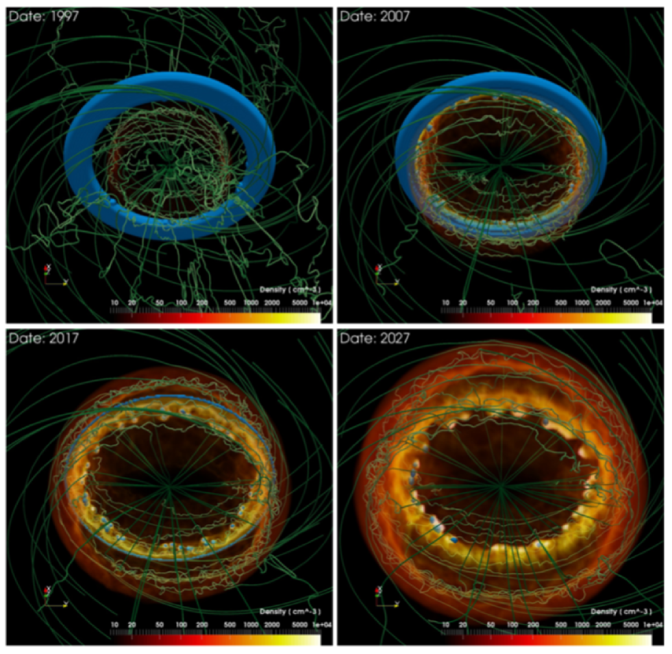
Figure 2: Three-dimensional volume rendering of the number density during the interaction of the blast wave with the magnetized nebula at the labeled times for model MOD-B1. The density of the shocked plasma is marked red and that of the unshocked equatorial ring material (with $n\geq 1000$ cm^-3) is marked blue. The green lines are sampled magnetic field lines; the scale of the magnetic field strength is log and is the same of Fig. 1. Refer to on-line Movie 1 for an animation of these data.

3 Results

As mentioned in Sect. 2, the first 24 hours in the post-explosion evolution of the SN are described by the best-fit model (run SN-M17-E1.2-N8) presented in Orlando et al. (2015). This model reproduces the main observable of the SN (i.e., bolometric lightcurve, evolution of line velocities, and continuum temperature at the photosphere). We refer the reader to Orlando et al. (2015) for a complete description of the evolution in this phase. Then we followed the transition from the SN to the SNR phase during the subsequent 40 years, including an ambient magnetic field. From the evolution of the remnant and its interaction with the nebula, we did not find any appreciable difference between the two cases considered, namely MOD-B1 and MOD-B100. In the following, therefore, we discuss in detail the results of run MOD-B1, mentioning the differences (if any) with the other case.

Figure 2 shows the evolution of number density during the interaction of the blast wave with the magnetized nebula for model MOD-B1. A movie showing the 3D rendering of plasma density (in units of cm^-3) distribution during the blast evolution is provided as on-line material (Movie 1). We found that the evolution in the present model (which includes the magnetic field) follows the same trend described in detail by the HD model of Orlando et al. (2015) and can be characterized by three main phases: an H II-region-dominated phase in which the fastest ejecta interact with the H II region (see upper left panel in Fig. 2; the unshocked H II region is not included in the rendering); a ring-dominated phase, in which the dynamics is dominated by the interaction of the blast wave with the dense equatorial ring (upper right and lower left panels; the unshocked ring is marked blue); and an ejecta-dominated phase, in which the forward shock propagates beyond the majority of the dense ring material and the reverse shock travels through the inner envelope of the SN (lower right panel).

3.1 Effects of the ambient magnetic field

As expected, the presence of an ambient magnetic field (of the assumed strength) does not change significantly the overall evolution of the remnant. In fact, for the values of explosion energy and ambient field strength considered, the kinetic energy of the shock is orders of magnitude larger than the energy density in the ambient $B$ field (even in MOD-B100). As a result, the magnetic field in the remnant interior is stretched outward by the expanding blast wave and assumes an almost radial configuration (see Fig. 2), at variance with the toroidal field in the pre-shock nebula (the Parker spiral; Fig. 1).

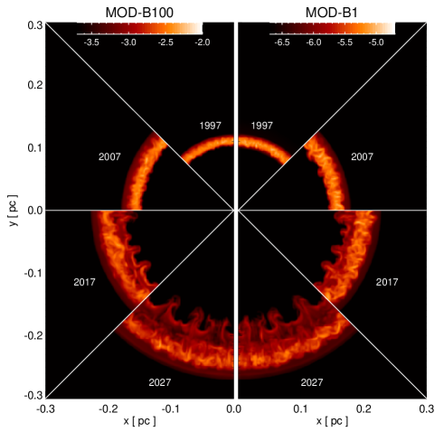
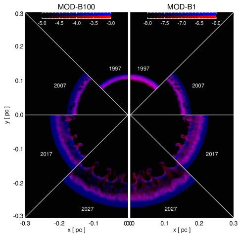
Figure 3: Upper panel: maps in the $(x,y)$ plane of maximum magnetic field strength along $z$ at the labeled times for MOD-B100 (on the left) and MOD-B1 (on the right). Lower panel: as in the upper panel, but for a two-color composite image showing the density averaged radial (red) and toroidal (blue) components of the magnetic field along $z$ (only shocked cells have been considered). The scale of the magnetic field strength is log and is given by the bar on the top of each panel, in units of $G$.

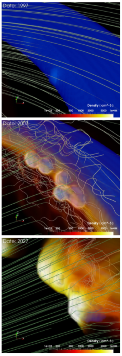
Figure 4: Same as in Fig. 2 for a close-up view of the interaction of the blast wave with the ring. Refer to on-line Movie 2 for an animation of these data.

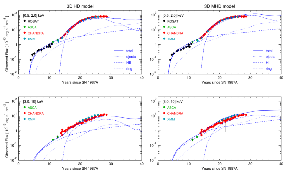
Figure 5: Comparison between observed (symbols) and synthetic (lines) X-ray lightcurves in the $[0.5,2]$ keV (upper panels) and $[3,10]$ keV (lower panels) bands for the best-fit HD model of Orlando et al. (2015) (left panels) and for the MHD model MOD-B1 presented here (right panels). Solid lines show the synthetic lightcurves; dotted, dashed and dot-dashed lines mark the contribution to emission from the shocked ejecta, the shocked plasma from the H II region, and the shocked plasma from the ring, respectively; the different symbols show the fluxes measured with Rosat (black diamonds; Haberl et al. 2006), ASCA (green; Orlando et al. 2015), Chandra (red; Helder et al. 2013; Frank et al. 2016) and XMM-Newton (cyan; Haberl et al. 2006; Maggi et al. 2012; Orlando et al. 2015).

In the mixing region between the forward and reverse shocks, the magnetic field follows the plasma structures formed during the growth of Rayleigh-Taylor (RT) instabilities at the contact discontinuity and shows a turbulent structure (see Fig. 2). The latter structure is enhanced even more by the expanding small-scale clumps of ejecta which modify the $B$ field in the mixing region (e.g. Orlando et al. 2012). The upper panel in Fig. 3 shows the maximum magnetic field strength along the $z$-axis for both MOD-B1 and MOD-B100; the lower panel shows the density-averaged radial (red) and toroidal (blue) post-shock components of $B$ along $z$. During the interaction of the blast wave with the nebula, the magnetic field strength can be locally enhanced by more than one order of magnitude, up to values of the order of $|B|_{\rm max}\approx 30\,\mu$G in MOD-B1 and $|B|_{\rm max}\approx 10\,$mG in MOD-B100, even if the back-reaction of accelerated CRs is neglected in our calculations (see upper panel in Fig. 3). This is mainly due to high compression of magnetic field lines in the post-shock. In addition, a significant radial component of $B$ appears in the mixing region, although the pre-shock nebula is largely dominated by the toroidal component (see lower panel in Fig. 3). This is due, on one hand, to RT instabilities developing at the contact discontinuity which lead to a preferentially radial component of $B$ around the RT fingers (e.g. Orlando et al. 2012) and, on the other hand, to stretching of the magnetic field trapped at the border of the ring and of the dense clumps by the plasma flow in the H II region. Interestingly, a recent detection of linear polarization of the synchrotron radio emission of SN 1987A suggests a primarily radial magnetic field across the remnant (Zanardo et al. 2018). Such a radial magnetic field seems to be a common feature in young SNRs (Dickel & Milne 1976; Dubner & Giacani 2015).

The magnetic field configuration is strongly modified during the interaction of the blast wave with the dense equatorial ring. Fig. 4 shows a close-up view of the interaction (the on-line Movie 2 shows the 3D rendering of plasma density, in units of cm^-3, during the blast evolution). As mentioned above, after the impact of the blast wave onto the ring, the magnetic field is trapped at the inner edge of the ring, leading to a continuous increase of the magnetic field tension there. Even if the plasma $\beta$ is, on average, larger than one (thus not affecting the overall evolution of the remnant), the field tension maintains a more laminar flow around the ring (and the denser clumps of the ring), limiting the growth of HD instabilities that would develop at the ring (and clumps) boundaries (see also, Mac Low et al. 1994; Jones et al. 1996; Fragile et al. 2005; Orlando et al. 2008). As a result, the magnetic field largely limits the progressive erosion and fragmentation of the ring and the latter survives for a longer time than if the magnetic field was not present (as it happens in the HD model of Orlando et al. 2015).

Since the thermal X-ray emission (especially in the soft band) is largely dominated by the shocked ring material during the ring-dominated phase (e.g. Orlando et al. 2015), we expect some changes in the X-ray lightcurves due to the presence of the magnetic field. Fig. 5 compares the X-ray lightcurves derived with our 3D MHD model (run MOD-B1) with those derived with the 3D HD model of Orlando et al. (2015); the symbols mark the observed lightcurves. In both cases, the transition from SN to SNR enters into the first phase of evolution (H II-region-dominated phase) about three years after explosion, when the ejecta reach the H II region and the X-ray flux rise rapidly. During this phase the two models (HD and MHD) produce very similar results and the effects of the magnetic field can be considered to be negligible: the models reproduce quite well the observed fluxes and slope of the lightcurves and the emission is dominated by shocked plasma from the H II region and by a smaller contribution from the outermost ejecta (dashed and dotted lines, respectively, in Fig. 5). This phase ends after $\approx 14$ years when the blast hits the first dense clump of the equatorial ring.

Around year 14 the SNR enters into the second phase of evolution (ring-dominated phase). At the beginning of the interaction with the ring (between year 14 and $\approx 25$), the two models show quite similar results, reproducing the observed lightcurves quite well, although the MHD model predicts slightly higher X-ray fluxes in the hard band. These higher fluxes are mainly due to higher fluxes from the shocked ring (compare dot-dashed lines in the lower panels of Fig. 5). After year 25, the differences in the fluxes predicted with the two models slightly increase with time: both soft and hard X-ray fluxes are higher in the MHD model than in the HD model. Again the differences originate mainly from the contribution to X-ray emission from the shocked ring. In the HD model, this contribution reaches a maximum between years 25 and 30; then, it decreases rapidly in both bands, and it is no longer the dominant component after year 34 when the SNR enters in the ejecta-dominated phase (see left panels of Fig. 5). Instead, in the MHD model, the contribution from the ring decreases slowly after the maximum around year 30 and it dominates the X-ray emission until the end of the simulation (year 40) when it is comparable to the contribution from the shocked ejecta (see right panels of Fig. 5). In the MHD model, the SNR enters in the ejecta dominated phase after year 40.

The differences in X-ray fluxes predicted by the HD and MHD models can be explained in the light of the effects of the magnetic field in reducing the fragmentation and destruction of the ring. In fact, in the MHD model, the magnetic field lines gradually envelope the dense clumps and the smooth component of the ring during the interaction with the blast wave (see Fig. 4 and on-line Movie 2), thus confining efficiently the shocked plasma of the ring and reducing the stripping of ring material by HD instabilities. As a result, the density of the shocked ring and, therefore, its X-ray flux are higher than in the HD model. The ring contribution to X-ray emission is evident in Fig. 6 which shows three-color composite images of the X-ray emission in the soft and hard bands integrated along the line of sight for the HD and MHD models at year 40 (namely when the differences between the two models are the largest). In the HD model, the ring is largely fragmented due to the action of HD instabilities developed in the ring surface after the passage of the blast and the emission is dominated by shocked clumps of ejecta. In the MHD model, the ring has survived the passage of the blast and is still evident after 40 years of evolution.

3.2 Evolution of the radio flux

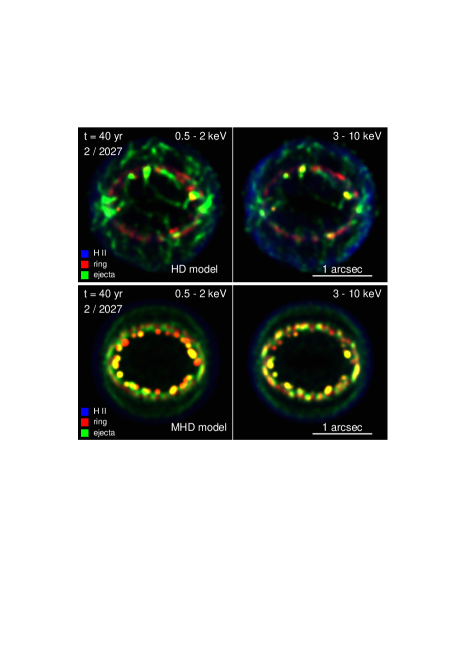
Figure 6: Three-color composite images of the X-ray emission in the soft ($[0.5,2]$ keV; left panels) and hard ($[3,10]$ keV; right panels) bands integrated along the line of sight at year 40 for the HD model of Orlando et al. (2015) (upper panels) and for the MHD model MOD-B1 (lower panels). Each image has been normalized to its maximum for visibility and smoothed with a Gaussian of size 0.025 arcsec. The colors in the composite show the contribution to emission from the different shocked plasma components, namely the ejecta (green), the ring (red), and the H II region (blue); yellow regions result from the combination of red and green.

From the model results we derived the non-thermal radio emission using REMLIGHT, as described in Sect. 2.3. The radio emissivity in Eq. 11 includes the term $C^{\prime}$ that was determined to fit the observations. We found that the shape of the lightcurves assuming either $b=0$ or $b=-1$ does not change appreciably. In the following, we discuss in more detail the case of $b=-1$ and the same conclusions can be applied to the case of $b=0$. We also found that, assuming either $\alpha=0.9$ or $\alpha=0.7$ (namely $\alpha$ is a constant), the synthetic lightcurves are much flatter than observed. In the following, we discuss the case in which $\alpha$ is given by Eq. 15. For our purposes, we assumed that $C^{\prime}$ in Eq. 11 does not depend on time (i.e. we did not consider its dependence on the spectral index $\alpha$; see Eq. 12).

Fig. 7 shows the synthetic flux densities (solid lines) calculated from models MOD-B1 and MOD-B100 plotted against observations at 2.4 GHz and 8.6 GHz. During the first 13 years of evolution, the observational data at the frequencies considered can be well reproduced by MOD-B1: the synthetic flux densities describe the sudden rise of radio emission occurring about three years after the SN (i.e. when the blast wave hits the inner part of the surrounding nebula) and the almost constant slope of the lightcurves observed in the subsequent years when the blast wave was traveling through the H II region and before its interaction with the dense ring. MOD-B100 reproduces the sudden rise of radio emission about three years after the SN but predicts, in the subsequent years, a slope of the lightcurves flatter than observed. Both models fail in reproducing the observations as soon as the blast wave hits the equatorial ring. MOD-B1 shows a significant steepening in the radio lightcurves after the blast wave hits the ring which is analogous to that observed in the soft X-ray lightcurve and at odds with radio observations (left panels of Fig. 7). A similar discrepancy between synthetic and observed lightcurves was found by Potter et al. (2014), synthesizing the radio emission from their 3D HD model. These authors proposed that the discrepancy might be explained if their model overestimates the mass of the ring and/or the ambient magnetic field within the ring. MOD-B100 shows lightcurves flatter than in MOD-B1 and in observations, reflecting the slower decrease of magnetic field strength with the radial distance from the center of explosion in the equatorial plane (see Fig. 1). Nevertheless, After year 10, MOD-B100 underestimates the observed flux density at the frequencies considered (right panels of Fig. 7).

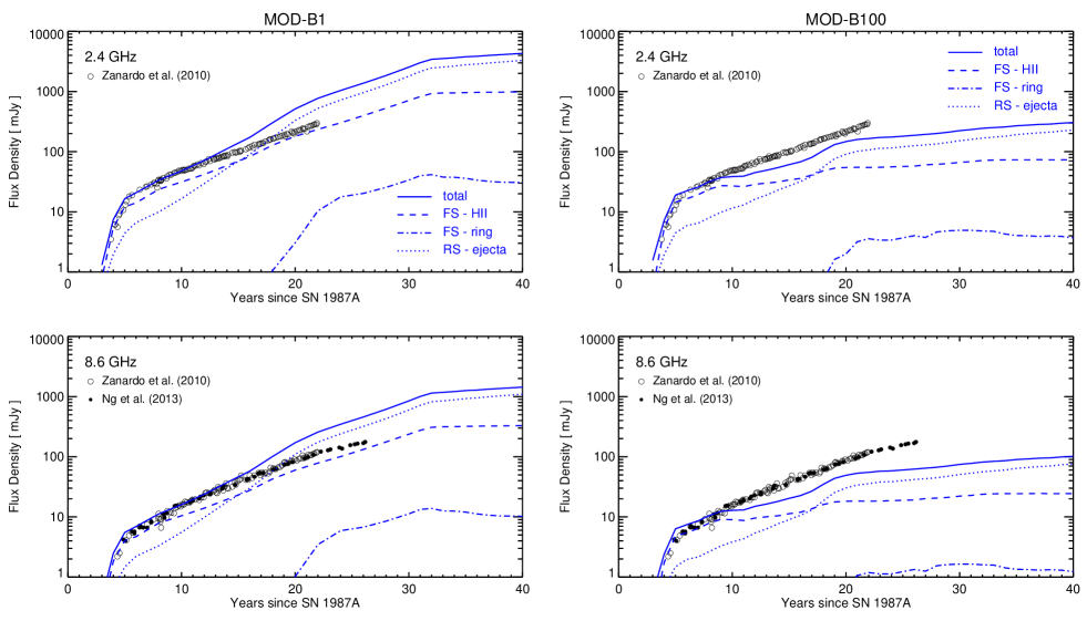
Figure 7: Synthetic radio flux densities (lines) for models MOD-B1 (left panels) and Mod-B100 (right panels) plotted against the observed ones (symbols) at 2.4 GHz (upper panels; Zanardo et al. 2010) and 8.6 GHz (lower panels; Zanardo et al. 2010; Ng et al. 2013). The figure shows the synthetic lightcurves (solid lines), the contribution to emission from the forward shock traveling through the H II region (dashed lines) and through the ring (dot-dashed lines), and the contribution from the reverse shock traveling through the ejecta (dotted lines).

Thanks to the passive tracers discussed in Sect. 2, we can identify the contributions to flux density which originate from the forward shock traveling through the H II region, from that traveling through the ring, and from the reverse shock traveling through the ejecta. Fig. 7 shows these contributions for the two models explored. We found that most of the emission originates from the forward shock traveling through the H II region (dashed lines in Fig. 7) and from the reverse shock traveling through the ejecta (dotted lines). The contribution from the shocked ring material (dot-dashed lines) is, at least, one order of magnitude lower than that from the other two components and, therefore, is negligible. In fact, even if the density ($n$) of the shocked ring is much higher (by an order of magnitude, on average) than that of the shocked plasma from the H II region, the volume ($V$) occupied by this plasma component is much lower (by a factor of $\approx 30$) than that of the shocked H II region. This together with the fact that the radio flux $F_{\mathrm{radio}}\propto nV$, whereas the X-ray flux $F_{\mathrm{X-ray}}\propto n^{2}V$, explain why the radio lightcurves are not dominated by emission from the shocked ring, at variance with the soft X-ray lightcurve which indeed is dominated by emission from the shocked ring material (cf. Fig. 5). Thus our results rule out the possibility that the models may overestimate the mass of the ring and/or the ambient magnetic field within the ring as suggested by Potter et al. (2014).

By inspecting Fig. 7, we note that a magnetic field configuration intermediate between those considered here might fit the observed lightcurves. In this case the radio emission may be dominated by the H II region during the first $\approx 15$ years of evolution and by the shocked ejecta at later times. On the other hand, Fig. 7 also shows that, in model MOD-B1, the steepening in the radio lightcurves around year 13 is caused by the contribution from the shocked ejecta (namely from the reverse shock) which becomes dominant about 15 years after the SN event, namely after the blast wave hits the equatorial ring. If this contribution were suppressed (at least by $\approx 2$ orders of magnitude) the observational data at both frequencies might be well reproduced by the model (see Fig. 8). In this case, the emission would be entirely dominated by the forward shock traveling through the H II region (the contribution from the shocked ring is orders of magnitude lower). The model would describe the sudden rise of radio emission occurring about three years after the SN and the almost constant slope of the lightcurves observed in the subsequent 27 years of evolution.

We note that Telezhinsky et al. (2012) have investigated the particle acceleration at forward and reverse shocks of young type Ia SNRs and found that reverse shock contribution to the cosmic-ray particle population may be significant. However, a dominant radio emission from the shocked H II region (and a negligible contribution from the shocked ring and from the reverse shock) is an interesting possibility because it might explain why the radio remnant (which, according to our model, shows the expansion of the blast wave through the H II region) expands almost linearly up to year 22 (Ng et al. 2008, 2013), in contrast with the X-ray remnant which shows a clear deceleration in the expansion around year 16 (Helder et al. 2013; Frank et al. 2016), namely when the X-ray emission becomes dominated by the emission from the shocked ring (Orlando et al. 2015; see Fig. 5). Also, this might explain why Ng et al. (2008) are able to fit the radio data more accurately by a torus model which can capture the latitude extent of the emission (due to the thickness of the H II region) rather than by a ring model (which is thinner), and why the radio remnant, dominated by emission from the shocked H II region, appears to be larger than the X-ray remnant which is dominated by emission from the slower shock traveling through the equatorial ring (Cendes et al. 2018). The above scenario is also supported by the findings of Petruk et al. (2017) who found that the thickness of the H II region in the 3D HD model of Orlando et al. (2015) fits well the evolution of the latitude extent of the radio emission (see their Fig. 6) derived by Ng et al. (2008, 2013).

3.3 A mechanism to suppress radio emission from the reverse shock?

In the light of the above discussion, a mechanism to suppress radio emission from the reverse shock may be invoked to reconcile models and observations. A hint to a possible mechanism comes from observations of the radio emission from SN 1987A: a number of authors inferred SSA to occur in the early expanding remnant of SN 1987A (e.g. Storey & Manchester 1987; Kirk & Wassmann 1992; Chevalier 1998). Thus we investigated if SSA or FFA might still play a role during the later interaction of the remnant with the nebula by using the 1D CR-hydro-NEI code (Lee et al. 2012, see Sect. 2.3). As initial conditions, we considered the radial profiles of density, pressure, velocity, and magnetic field strength derived from model MOD-B1 in the plane of the ring about one year after the SN event (namely before the interaction of the blast wave with the nebula). We evolved the system for 30 years, deriving the radio lightcurve in the 2.4 GHz. We found that SSA does not play any significant role in the model in the period between years 3 and 30. This is mainly due to the fact that the magnetic field is never remarkably large both for the shocked ejecta and CSM. FFA does cut off the lower frequencies for both ejecta and CSM emission at a comparable level, but it does not affect the spectrum around 2.4 GHz (and at larger frequencies). This is in agreement also with previous studies on the role of SSA and FFA in the late radio emission from SN explosions (e.g. Pérez-Torres et al. 2001): at frequencies higher than 1 GHz these effects are negligible after $\sim 1400\ {\rm days}\sim 4\ {\rm yrs}$ since the SN.

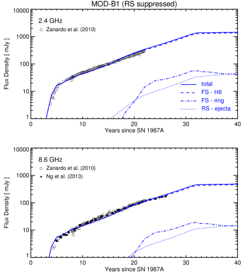
Figure 8: As in Fig. 7 for model MOD-B1 and assuming the emission from the reverse shock reduced by two orders of magnitude.

The 1D CR-hydro-NEI simulations show that a very strong boost of radio emissivity from the ejecta is resulted from their interaction with the nebula (to a larger extent than the forward shock emission). Following a strong compression of the shocked ejecta due to the rapid deceleration of the forward shock and to the feedback of accelerated particles (which is included in CR-hydro-NEI calculations), the reverse shock is highly strengthened and pushed into the high density envelope of the ejecta, resulting into a rapid increase of accelerated electrons in the ejecta. This explains why, if the diffusive shock acceleration (DSA) efficiency at the reverse shock is not suppressed, the radio flux from the ejecta can easily overshoot the observed flux as also found with the synthesis of radio emission from the 3D MHD simulations (see Fig. 7). On the contrary, if the DSA at the reverse shock is highly suppressed, the model can reproduce the observed lightcurves, thus strongly favoring a shocked CSM (forward shock) origin of the radio emission, in agreement with the findings of Fig. 8. In such a case, the acceleration efficiency at the reverse shock might be strongly constrained.

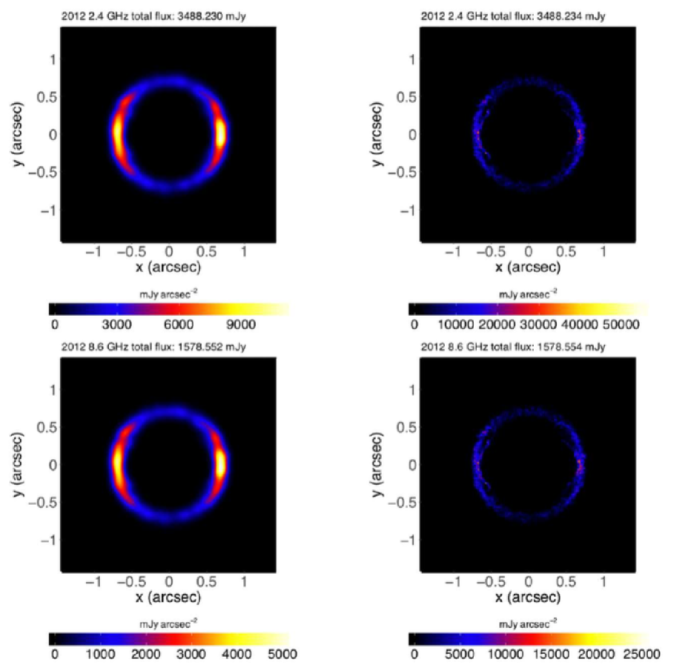
Figure 9: Synthetic maps at 2.4 GHz (upper panels) and 8.6 GHz (lower panels) for the 2012 epoch (24 years after the SN) from the model MOD-B1. The left column shows the images convolved by a beam with FWHM of 0.5 arc seconds, while the right column shows the unconvolved images. The total flux in convolved images is the same of that in unconvolved images.

The CR-hydro-NEI code assumes spherical symmetry in the expansion of the remnant and it cannot describe the inhomogeneous structure of the nebula around SN 1987A. In particular it does not describe the complex configuration of the magnetic field when the blast wave runs over the dense ring (see Sect. 3.1). Thus, to investigate further the role played by SSA in the radio evolution of SN 1987A, we used the SPEV code (Mimica et al. 2009; see Sect. 2.3) to synthesize, from run MOD-B1, the radio emission at 2.4 GHz and 8.6 GHz. Fig. 9 shows an example of radio maps obtained with SPEV for year 24 (i.e. the 2012 epoch), assuming isotropic injection. We found that some absorption of emission from the reverse shock can be present in correspondence of the equatorial ring, especially at 2.4 GHz. This is mainly due to the dense material of clumps with number density $\approx 10^{4}$ cm^-3 and temperature around $10^{4}$ K. Nevertheless this absorption reduces the emission from the reverse shock by only a few percents and it is not able to account for a significant suppression of the radio flux.

In the synthesis of radio emission, we have assumed that the parameter $C^{\prime}$ is the same for forward and reverse shocks ($C^{\prime}_{\mathrm{FS}}=C^{\prime}_{\mathrm{RS}}$). This parameter describes the contributions to the radio emission from electron populations accelerated by the shock. However, as shown in Fig. 8, the radio lightcurves can be reproduced by our model if the DSA at the reverse shock is highly suppressed. The parameter $C^{\prime}$ is linked to the number of particles available for the acceleration and to the magnetization of the pre-shock medium. In the case of SN 1987A, many authors suggest that the unshocked ejecta should be mainly in neutral or in singly ionized states (e.g. Jerkstrand et al. 2011). In this case, very few particles should participate in the process of acceleration at the reverse shock. However, once the ejecta is crossed by the reverse shock, the material is heated up to temperatures of several millions degree and ionized, possibly introducing fresh particles available for acceleration. It is more likely, therefore, that $C^{\prime}_{\mathrm{RS}}<<C^{\prime}_{\mathrm{FS}}$ due to a different magnetization of plasma. In fact, first principle particle-in-cell (PIC) simulations of perpendicular strongly magnetized shocks have shown that accelerated electrons can be heavily suppressed as a consequence of the lack of sufficient self-generated turbulence (e.g. Sironi et al. 2013).

According to Sironi et al. (2013), the maximum Lorentz factor at saturation for the electrons, $\gamma_{sat,e}$, in a relativistic magnetized shock in an electron-proton plasma is

$$\gamma_{sat,e}\approx 2\gamma_{0}\frac{m_{i}}{m_{e}}\sigma_{m}^{-1/4},$$ (16)

where $\gamma_{0}$ is the Lorentz factor, $m_{i}$ and $m_{e}$ are the masses of ions and electrons, respectively, and $\sigma_{m}\approx 50B^{2}n^{-1}$ is the magnetization calculated as the ratio of magnetic to kinetic energy density. Sironi et al. (2013) have shown that, with increasing magnetization, the acceleration efficiency decreases: if the magnetization in the pre-shock is larger than $\approx 10^{-4}$, the post-shock spectrum does not show any evidence for non-thermal particles and the radiation in the bands of interest is strongly suppressed. In the case of SN 1987A (which is non-relativistic), we expect that the critical value of $\sigma_{m}$ at which the radio emission is suppressed might be different. Nevertheless, if the unshocked ejecta is more magnetized than the CSM, and if it is above some critical value, this could be an argument in favor of suppression of the reverse shock emission. However, in model MOD-B1, the reverse shock magnetization is lower than that of the forward shock. Also $\sigma_{m}<5\times 10^{-6}$ in the ejecta, too low to make a difference in $\gamma_{sat,e}$ in enough emitting volumes; in fact we found that the difference in flux is at the level of 0.1%.

On the other hand, $\sigma_{m}$ increases as $B^{2}$. For instance, by increasing $B$ in the unshocked ejecta of our model by a factor of 100, $\sigma_{m}$ should be a factor of $10^{4}$ larger. Thus more magnetized models (especially in the ejecta) would yield a limit for the maximum Lorentz factor that would forbid the emission at radio frequencies in the reverse shock. We suggest, therefore, that the model considered here underestimates the magnetic field strength in the ejecta so that the radio emission is not suppressed at the reverse shock. Zanardo et al. (2018) found a magnetic field strength of a few mG in the region between the forward and reverse shocks in SN 1987A. If the magnetic field strength in the ejecta is of the order of that inferred from the observations, $\sigma_{m}$ might large enough to provide a natural explanation for the suppression of radio emission from the reverse shock.

We note that our model assumes a magnetic field strength and configuration in the initial remnant interior (at $t\approx 24$ hours since the SN) which are derived from the Parker spiral model (which is appropriate for the CSM). We expect, however, that a more realistic field (especially in the immediate surroundings of the remnant compact object) would be much more complex than that adopted here and it should reflect the field of the stellar interior before the collapse of the stellar progenitor. Unfortunately we do not have any hints on this magnetic field. Also, it is likely that efficient field amplification by MRI occurred after core bounce (e.g. Obergaulinger et al. 2018). We conclude that, most likely, we are largely underestimating the strength of this magnetic field.

4 Summary and conclusions

We modeled the evolution of SN 1987A with the aim to investigate the role played by a pre-SN ambient magnetic field in the dynamics of the expanding remnant and to ascertain the origin of its radio emission. To this end, we developed a 3D MHD model describing the evolution of SN 1987A from the immediate aftermath of the SN explosion to the development of the full-fledged remnant, covering 40 years of evolution since few hours after the SN event. The model considers a plausible configuration of the pre-SN ambient magnetic field and includes the deviations from equilibrium of ionization, and the deviation from temperature-equilibration between electrons and ions. The initial condition is the output of a SN model able to reproduce the bolometric lightcurve of SN 1987A during the first 250 days of evolution. The nebula around SN 1987A is modeled as in Orlando et al. (2015), adopting the parameters of the CSM derived by these authors to fit the X-ray observations (morphology, lightcurves and spectra) of the remnant during the first 30 years of evolution. Our findings can be summarized as follows.

1. The presence of an ambient magnetic field does not change significantly the overall evolution and the morphology of the remnant. The 3D MHD model reproduces the X-ray morphology and lightcurves of SN 1987A during the first 30 years of evolution, by adopting the same initial condition (the SN model) and boundary conditions (the geometry and density distribution of the nebula around SN 1987A) of the best-fit HD model of SN 1987A presented in Orlando et al. (2015).

2. The magnetic field plays a significant role in reducing the erosion and fragmentation of the dense equatorial ring after the passage of the SN blast wave. In particular, the field maintains a more laminar flow around the ring, limiting the growth of HD instabilities that would develop at the ring boundary. As a consequence, at variance with the results from the HD model, the ring survives the passage of the blast until the end of the simulation (40 years). The ring contribution to thermal X-ray emission is slightly higher than that in the HD model and is the dominant component until the end of the simulation (40 years after the SN event).

3. The two models explored (MOD-B1 and MOD-B100) predict different slopes of the radio lightcurves due to different radial variations of the magnetic field strength considered in the two cases. MOD-B1 is able to fit the radio lightcurves of SN 1987A during the first 13 years of evolution, namely when the blast wave travels through the H II region. In that period most of the radio emission originates from the forward shock traveling through the H II region. At later times, the model predicts a significant contribution to the radio flux originating from the reverse shock. This contribution becomes dominant after the blast wave hits the equatorial ring (about 15 years after the SN event). However, this contribution leads to a steepening in the radio lightcurves at odds with observations. MOD-B100 predicts a slope of the lightcurves flatter than that observed already at early times ($\approx 5$ years after the SN) and it is not able to fit the observed lightcurves. In both models, the radio flux arising from the shocked ring material is negligible because the volume occupied by this plasma component is much smaller than that of the shocked H II region.

4. MOD-B1 may reproduce the radio lightcurves over the whole observed period if the flux originating from the reverse shock was heavily suppressed (by $\approx 2$ orders of magnitude; see Fig. 8). We explored if SSA and/or FFA could be possible candidates for the absorption mechanism of the radio emission and we found that they do not play any significant role in the model after 3 years since the SN. On the other hand, the magnetic field strength and configuration adopted in our model are arbitrary (the only constraint is the field strength at the inner edge of the nebula), especially in the remnant interior where the field should reflect that of the stellar interior before the collapse of the progenitor star. We suggest that a larger magnetic field in the unshocked ejecta would yield a limit for the maximum Lorentz factor that would forbid the emission at radio frequencies in the reverse shock.