R-band light-curve properties of Type Ia supernovae from the (intermediate) Palomar Transient Factory

Abstract

We present the best 265 sampled R-band light curves of spectroscopically identified Type Ia supernovae (SNe) from the Palomar Transient Factory (PTF; 2009-2012) survey and the intermediate Palomar Transient Factory (iPTF; 2013-2017). A model-independent light curve template is built from our data-set with the purpose to investigate average properties and diversity in our sample. We searched for multiple populations in the light curve properties using machine learning tools. We also utilised the long history of our light curves, up to 4000 days, to exclude any significant pre- or post- supernova flares. From the shapes of light curves we found the average rise time in the R band to be $16.8^{+0.5}_{-0.6}$ days. Although PTF/iPTF were single-band surveys, by modelling the residuals of the SNe in the Hubble-Lemaître diagram, we estimate the average colour excess of our sample to be $<$E$($B$-$V$)>\approx 0.05(2)$ mag and thus the mean corrected peak brightness to be $M_{R}=-19.02\pm 0.02$ $+5\log({\rm H}_{0}[{\rm km}\cdot{\rm s}^{-1}{\rm Mpc}^{-1}]/70)$ mag with only weakly dependent on light curve shape. The intrinsic scatter is found to be $\sigma_{R}=0.186\pm 0.033$ mag for the redshift range $0.05<z<0.1$, without colour corrections of individual SNe. Our analysis shows that Malmquist bias becomes very significant at z=0.13. A similar limitation is expected for the ongoing Zwicky Transient Facility (ZTF) survey using the same telescope, but new camera expressly designed for ZTF.

1 Introduction

Type Ia supernovae (SNe) are understood by now to be thermonuclear explosions of white dwarfs. However, the mechanism of the explosion remains unknown. The leading theories involve binary interaction with two different scenarios; the single degenerate (SD) and the double degenerate (DD) scenario involving a giant or main sequence companion star or a white dwarf companion, respectively (see Maeda & Terada, 2016, for a recent review). Despite the lack of theoretical certainty about progenitors, type Ia SNe have proven very useful in cosmology as “standardisable" distance estimators, which led to the discovery of the accelerating expansion of the universe (Riess et al., 1998; Perlmutter et al., 1999) attributed to the existence of a new cosmic constituent dubbed “dark energy" (see Goobar & Leibundgut, 2011, for a review).

Following the discovery of dark energy, many studies have focused on increasing the precision and accuracy of the cosmological parameters derived from type Ia SNe combined with other cosmological probes (e.g. Betoule et al., 2014; Scolnic et al., 2017). Both statistical and systematic uncertainties need to be improved to discern between dark energy models, see e.g. Dhawan et al. (2017). The systematics include, but are not limited to possible brightness evolution over cosmic time, cross-calibration of different instrument, telescope data and properly accounting for extinction by dust in the line of sight. One way to study the systematic uncertainties is to investigate large samples of nearby and distant SNe, as shown in many works in the literature, e.g. by the SDSS-II and SNLS collaborations (Kessler et al., 2009; Sullivan et al., 2011; Betoule et al., 2014). Other important contributions include results from PTF (Maguire et al., 2014), the Supernova Cosmology Project (SCP, Amanullah et al., 2010; Suzuki et al., 2012) and from PanSTARRS1 (Rest et al., 2014). Another approach to better understand systematics is to study nearby individual SNe to probe the SN physics. Examples of such studies based on Palomar Transient Factory (PTF) and its successor, the intermediate Palomar Transient Factory (iPTF) include Nugent et al. (2011), Dilday et al. (2012), Goobar et al. (2014), Goobar et al. (2015), Cao et al. (2015), Hsiao et al. (2015) and Miller et al. (2017).

In this paper we use a large homogeneous data set of low-redshift SNe Ia in a single photometric band from the Palomar 48-inch Oschin Schmidt Telescope to address some of the uncertainties associated with their use in cosmology. PTF and iPTF were two surveys dedicated to finding, among other things, SNe within days from explosion (Rau et al., 2009). The survey imaged hundreds of square degrees of the sky, twice or more times per night. This enabled us to build light curves of the transients, i.e., follow their brightness over time. Through this strategy two different time scales were probed simultaneously: a longer one over the years the survey ran and a shorter intra-night timescale. The large field of view of the PTF/iPTF, 7.26 deg², allowed us to cover a large part of the sky and thus building a statistical sample of type Ia supernovae detected in a similar fashion, and minimizing selection effects.

We present observations in the R band for the SNe with the most complete coverage. These are used to explore the light curve properties and possible signs of yet unknown diversity among SNe Ia. For the light curve as a whole, we use a non-parametric fitting method, Gaussian processes, to generate a smooth version of the light curves in order to look for signs of multiple SN Ia populations and to study intrinsic dispersion at different epochs (see Section 3). In the same Section, we also use the light curves in 3 different redshift bins to look for diversity in a given epoch at different cosmic times. We present average photometric properties of the sample, e.g., the rise-time distribution light curve (Section 4.2), and the dispersion of the light curves at various epochs (Section 3.2). We utilise the long history of detections before and after the supernova light is visible to set limits on a pre- and post-explosion event in Section 4.1. From the distribution of residuals in the Hubble-Lemaître diagram, we explore if there is a correlation with light curve shape in the R band (Section 5) and the stellar mass of the host galaxy (Section 5.3). Furthermore, we estimate the mean free path due to scattering by dust along the line of sight, even without colour information.

In a follow-up paper we will present the spectra used to classify the SNe and determine the redshift of the SNe in this study, as well as detailed a analysis of their spectroscopic properties, and use machine learning techniques to relate these to the photometric properties shown in this work.

2 The data set

2.1 The PTF and iPTF transient surveys

PTF and iPTF surveyed the sky regularly to discover new transients with an unprecedented large field of view. The survey was conducted in a single filter at a time, mostly in the Mould R band (wavelength range $5800$-$7300$ Å), but data in g band (wavelength range $3900$-$5600$ Å) were also collected during some periods. Narrow $H_{\alpha}$ filters at several recession velocities were used during the 2-5 days closest to the full moon each month. The magnitude limit of the survey was 20.5 and 21 magnitudes for R and g band respectively in the PTF system. In this paper, we focus on the R-band observations.

PTF and iPTF performed a non-targeted survey by imaging the sky 1-5 times per night with exposures on the same field (at least 40 minutes apart) and then performing difference imaging, in order to discover new transients. 50% of the observations are taken with a 1 day cadence or shorter and 70% within 4 day cadence excluding the intra-night cadence which is the most common (43 or 63 minutes apart). The reference images were taken in 2009 and 2012 for PTF and iPTF, respectively, for the majority of the fields. A non-targeted survey means that no particular part of the sky was imaged in the survey, thus minimising the bias associated with targeted searches, e.g. finding transients only in well-resolved host galaxies. In addition, since we use data only from a single instrument and photometric band, other systematic effects are minimised. This makes PTF and iPTF ideal for minimising the sampling bias.

After running through an image-subtraction pipeline the measured parameters from the extracted sources were analysed using a machine learning algorithm (Bloom et al., 2008). This algorithm sets a score on the likelihood that each candidate is an astrophysical transient, which is used to discard the many false candidates that are found by the pipeline. For the PTF collaboration, this was done in a combination of “Supernova zoo participants" (Smith et al., 2011) to train the algorithm and an effort of the collaboration where the top candidates were screened by team members and sent for spectroscopic follow-up. The overall supernova detection performance of the PTF survey is explored in Frohmaier et al. (2017) and the iPTF survey efficiency estimation is work in progress. For the iPTF data the top candidates were selected solely by people from the collaboration.

This survey strategy and rapid follow-up enabled discoveries of transients close to the last non-detection limits. The mean of the first detection point in time for our SNe is -12 days, compared to -4 days in the low redshift sample presented by Betoule et al. (2014). A histogram of the first detection points of both surveys is shown in Figure 8 in Section 5, where the implications are also discussed.

2.2 Photometry and Calibration

All photometric data used in this paper are in the Mould R band (see Law et al., 2009, and Appendix A), corrected for quantum efficiency of the instrument. The PTF image processing is described in Laher et al. (2014). We used the PTF-IPAC forced photometry pipeline by Masci et al. (2017), to produce the light curves. The procedure to process the PTF-IPAC pipeline photometry in light curves used in our analysis is described in detail in Appendix B.

The photometric pipeline performs difference imaging on a fixed position, in this case, the position of the supernova as determined at discovery, to remove the host galaxy contamination. A point spread function (PSF) fit is then performed at this position for each of the images. Where calibration against images from the Sloan Digital Sky Survey (SDSS) was not possible, a field observed during the same night was used.

The error estimates of each data point take into account the goodness of fit of the PSF, the overall zero point at the time of observation as compared to SDSS wherever possible in order to get the absolute photometry. Note that the magnitudes used in this paper are magnitudes are in the PTF system (rather than the AB system, see conversion formulae in Ofek et al., 2012), and thus have not been corrected for the colour of SNe Ia. The repeatability between different CCD chips for the same stars is better than 0.03 mag in 95% of cases, see Ofek et al. (2012). There are additional systematics that were deemed sub-dominant, including incorrect PSF template estimation, uncertainties in the SN position and astrometric calibration which determine the central position of the PSF fit.

2.3 The type Ia SNe sample

In this paper we examine the statistical properties of 265 out of 2059 spectroscopically confirmed type Ia supernovae from PTF and iPTF (from 2009-2017), selected due to their well sampled R-band light curves (see criteria in Section 3). We do not exclude any SNe based on their spectroscopic sub-classification. Due to the observing strategies in 2015 and 2017 no SN Ia was included from these years.

We classify the supernovae using Supernova Identification software SNID (Blondin & Tonry, 2007) using the version 2.0 templates. We select the 5 best fits that pass the SNID criteria “good" and choose the most common type from these. We then visually inspect the best fits to be certain of the typing.

For 169 of the SNe in our sample, the redshift is measured from host galaxy lines in the SN spectra or from the host spectrum. When this is not available we use the SDSS spectral redshift (15 SNe) of the host galaxy or host redshifts from NED (3 SNe) and if that is not available the median redshift of the 5 best estimates from SNID is used (56 SNe). We note that to have a precise redshift the hosts would have to be revisited to get a more accurate redshift.

In Figure 1 we show the spatial distribution on the sky of the data sample. Due to weather constraints a larger portion of well-sampled SNe are from the spring/summer half of the year. The gap in data on the northern hemisphere is from the galactic plane which obscures extragalactic SNe. The area around the galactic plane is also very crowded, i.e. filled with many stars, and thus harder to perform accurate image subtractions to find transients.

Figure 1: Right-ascension (RA) and declination (Dec) distribution of the type Ia supernovae from the PTF and iPTF surveys. In yellow points we see the 265 best sampled SNe used in this work, the black points show the rest of the type Ia SNe from the PTF and iPTF surveys. The empty regions is the location of our Milky Way galaxy and the southern hemisphere.

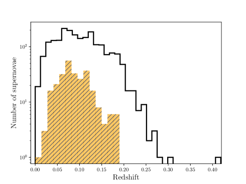
Figure 2: Redshift distribution of the PTF and iPTF SNe Ia sample. In the shaded region we show the distribution for the most well-sampled SN Ia used in this work. Note iPTF16geu, at redshift 0.4 as a significant outlier (Goobar et al., 2017).

In Figure 2 we show the redshift distribution of our data sample in shaded and in comparison to the entire PTF and iPTF sample of type Ia SNe.

3 light curves and building a template

The norm in modern cosmology with type Ia SNe is to fit a time-evolving spectral energy distribution (SED) to the light curves to extract parameters used to derive their distance,e.g. MLCS2k2 (Jha et al., 2007), BayeSN (Mandel et al., 2011), SALT2 (Guy et al., 2007) , SIFTO (Conley et al., 2008) and SNooPy (Burns et al., 2011). In order to use our data instead of a parametrized template to fit our SNe, we here use a model that does not impose a pre-defined form to construct an empirical model template. The template is used to extract parameters such as peak magnitude and stretch, but also to study the intrinsic dispersion at different epochs along the light curves. This method, Gaussian processes, has been used for type Ia SN cosmology previously ( in e.g. Holsclaw et al., 2010b; Kim et al., 2013; Shafieloo et al., 2013a; Cao et al., 2016) but not for large samples, mainly due to its computationally intensive nature. We start by aligning the light curves in Section 3.1 and then perform Gaussian processes in Section 3.2 to obtain a template and study the light curve parameters. Throughout this paper we use the code packages Astropy version 2.0.4 (The Astropy Collaboration et al., 2018), Matplotlib (Hunter, 2007), Scipy (Jones et al., 2001) version 1.0.0, numpy version 1.14.1 and sncosmo version 1.5.3 (Barbary, 2014) for our data analysis.

3.1 Quality cuts and aligning the light curves

We align the light curves in time and normalise their magnitudes, such that zero is the peak magnitude.

The following conditions have been set for the supernovae included in the sample:

• More than 10 data points in the light curve, at least 3 before and 5 after time of peak.

• At least 4 points within $\pm 5$ days of the peak.

• Data spanning at least 15 days.

• Not located in a known quasar or active galactic nucleus (AGN).

From the 2059 spectroscopically confirmed SNe Ia in the survey we had 1705 in the R-band from these we apply the first cut with data from the Nugent photometric pipeline (an aperture photometry pipeline) that was the real-time pipeline used in the surveys and the remaining cuts with the PSF based PTF-IPAC pipeline. 1104, 133, 70 and 7 SNe are cut by the first, second, third and fourth condition respectively. The reason for having such strict constraints is to ensure an accurate template and be well-sampled enough to probe the different science questions investigated further in the paper, such as early light-curves. In future work less strict cuts can be made for different science cases. The first, second and third conditions are there to pinpoint the peak and the fourth to eliminate high intrinsic noise in supernovae light curves caused by their environment. The last condition only accounts for registered AGN activity in the host galaxy. For the case of SN 2014J (or iPTF14jj) we exclude this from our light curve template analysis due to saturated data point, however we include it in Section 4.1 since that part of the light curve is unaffected by the saturated points.

First, the peak of the light curve was estimated by using the brightest point in the light curve and then fitting the interpolation of a well sampled supernova from our sample, PTF10hmv, and selecting the peak that minimises $\chi^{2}$. We then check that the conditions are fulfilled and correct the remaining light curves for cosmological time-dilation and align in them in time and magnitude according to this initial peak estimate.

From this initial alignment we now K-correct the light curves, apply our cuts and minimise the modified ${\chi^{2}}$,

$$\mathcal{Q}^{2}=\left.{\displaystyle\sum_{i}^{N}\left(\frac{m_{i}-m_{T}(d_{i}+\delta t)+A}{\sigma_{phot,i}}\right)^{2}}\middle/\right.N^{4},$$ (1)

over the parameters time $\delta t$, and magnitude normalisation $A$. $m_{T}(t)$ is the magnitude of the template at time $t$, $(d_{i},m_{i})$ are the normalised times and magnitudes and $\sigma_{phot,i}$ is the photometric error.

Since only the points between -20 and +100 days with respect to maximum light contribute to the $\chi^{2}$, we can trivially obtain a perfect fit by shifting the points until only one is left in range. To counteract this, we need to encourage the loss function to include points. One possible way is to include some penalty for bright points outside of the range, but this would not be effective since there are some photometric artefacts. Instead, we decided to explicitly reward the inclusion of points by dividing $\chi^{2}$ by $N^{2}$. Several other factors were tried (such as $N$, $N^{3}$, $\sqrt{(}N)$…), but $N^{2}$ yielded the most well-aligned light-curves. Higher factors, like $N^{3}$, compress the light-curve in order to add more points, while lower factors like $N$ and $\sqrt{(}N)$ suffer similar problems to a normal $\chi 2$. This has the consequence of adding a bias on the stretch factor of the SNe which we avoid by using the $N^{2}$ factor. This initial template is made with data from -20 days to +80 days since this is the interval for which we have K-corrections and sufficient data. The K-correction (Oke & Sandage, 1968; Kim et al., 1996) takes the observed magnitude and converts into the magnitude it would have had in a common rest-frame which requires the SED of a supernova. We used the SED of Hsiao et al. (2007) consisting of about 600 spectra in the time span of -20 to +85 days with respect to B-band maximum, and adapted equation 2 in Oke & Sandage (1968) for K-corrections in the same band, in this case the P48 R-band, $K_{R}$. Here $F(\lambda)$, $S_{R}(\lambda)$ and $z$ are the spectral energy distribution for a given wavelength $\lambda$, the filter transmission for the same wavelength and redshift respectively.

$$K_{R}=2.5\log_{10}(1+z)+2.5\log_{10}\left(\frac{\int F(\lambda)S_{R}(\lambda)d\lambda}{\int F\left(\frac{\lambda}{(1+z)}\right)S_{R}(\lambda)d\lambda}\right)$$ (2)

The K-correction in R-band evolves with epoch and vary between -0.01 and -0.35 magnitudes (for z=0.2). For the entire PTF and iPTF samples the mean K-correction is -0.25 magnitudes. Uncertainty in K-corrections is expected to be larger for peculiar supernovae since the template is made with “normal" type Ia supernovae. We estimate the error in our K-corrections by comparing our fits to SALT2 fits.

We fit the SALT2 model to the (i)PTF r-band lightcurves using sncosmo. Since we were only using data in a single band, we fixed the color parameter $c$ to 0 but applied observer-frame extinction based on Milky Way dust. Most lightcurves contain limits from observations of their location that were made years before and/or after the SN exploded. Since we do not gain much for the SALT2 fit from most of those limits, we discarded any data 30 days before the first data point with $S/N>5$ and 30 days after the last point with that significance. Based on the best-fit values for the remaining parameters we then calculated the rest-frame peak brightness in r-band (as well as the standard B-band). When calculating the the $\chi^{2}$-values listed in Table LABEL:table:salt2, we excluded the points that fall outside the definition range of the SALT2 model that was fit (and which otherwise would lead to very low values of $\chi^{2}$/d.o.f. because the limits will perfectly match the model flux, which is set to zero outside the definition range). We then use these fits to estimate the K-correction error by fitting a Gaussian to the difference between the maximum magnitude from the SALT2 fits and our fits to get the variance between the two, which is found to be 0.046 mag. This is a conservative estimate, as other sources of error cannot be excluded.

When this first fitting has been done, we make sure that the conditions are still fulfilled, and then proceed to doing a second fit. This time another free parameter is allowed, measuring the light curve width, stretch $S$. Stretch is defined to be a multiplicative factor that measures the width of the light curves, thus $S<1$ implies a narrow shape, $S>1$ a broad shape and $S=1$ a shape that exactly matches that of the template similar to what was done in Perlmutter et al. (1997). The time $t$ in days is thus defined to be,

$$t=t_{0}\times S.$$ (3)

The light curves are fitted to the template created from the first fit minimising

$$\tilde{Q}^{2}=\left.{\displaystyle\sum_{i}^{N}\left(\frac{m_{i}-m_{T}(d_{i}\times S+\delta t)+A}{\sigma_{phot,i}}\right)^{2}}\middle/\right.{N^{4}},$$ (4)

over the parameters $A$, $\delta t$ and $S$.

As shown in the upper panel of Figure 3 we see the final 265 aligned and averaged SNe and in the lower panel of Figure 3 the same but binned in 3 redshift ranges.

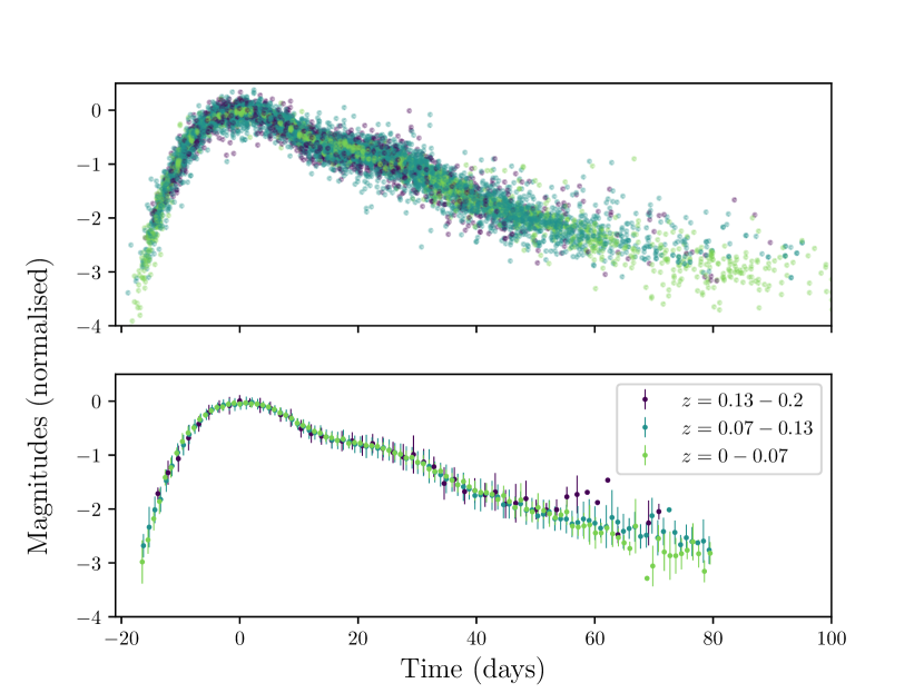
Figure 3: All aligned light curves. The data points are colour-coded according to redshift as shown in the legend. In the upper panel, we show the un-binned data and in the lower panel we show binned data points, in 3 redshift ranges.

From the starting sample of 2059 supernovae, 265 remained at the end for the R-band after quality cuts were applied. Table 1 shows at what stage the supernovae drop out. The first step selects the R-band light curves with the initial maximum estimate of maximum light to fulfil the conditions.

Table 1: Total number of SNe in the sample after each respective process in preparing the light curves for the template.

Process	Number of SNe
Conditions met using initial maximum	391
K-corrections & fitting of maximum	344
Stretch correction added	265

We correct for Milky way extinction at the position of the supernova using the maps of Green et al. (2018), implemented in the package dustmapsto get E(B-V), i.e. the colour excess. We then use,

$$A_{R}=\frac{A_{V}}{R_{V}}\frac{\lambda_{B}}{\lambda_{R}}\left(\frac{\lambda_{V}-\lambda_{R}}{\lambda_{V}-\lambda_{B}}\right)+A_{V}$$ (5)

to find the extinction in the R-band, $A_{R}$ due to Milky way extinction. We assumed the total-to-selective extinction parameter, $R_{V}=3.1$. Here $\lambda_{i}$ is the central wavelength in the $i^{th}$ band and $A_{V}$ is the extinction in the V-band. The average is found to be $0.095$ magnitudes in the R-band.

We do not set an upper limit requirement on $A_{V}$ in our sample, hence the largest galactic E(B-V) among our SNe is 0.79 mag compared to the 0.15 mag limit set by Betoule et al. (2014) for inclusion in the Hubble-Lemaître diagram.

After these corrections the last step performs in addition a stretch correction and refits for the peak magnitude. At all processes the conditions to be fulfilled are rechecked. We find the root-mean-squared, rms of the aligned light curves (for all epochs) to be $0.19$ magnitudes within 5 days of the peak. The result of the aligned light curves are shown in Figure 3.

3.2 Gaussian Processes template

In order to get a predictive light curve template we have used Gaussian processes (GP). This method allows a non-parametric way to estimate, based on the training data (our dataset), what the predicted behaviour will be for a supernova and in addition allows deviation from this to be quantified. This method has been applied to supernova cosmology before by Shafieloo et al. (2013b), Holsclaw et al. (2010a) and for modelling type Ia supernovae in Kim et al. (2013). Since Gaussian processes decay to zero outside of the data range, we perform the fitting in flux space.

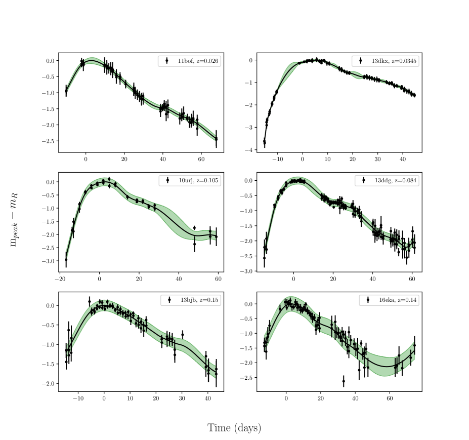
Figure 4: Six example light curves with their Gaussian processes fit with normalised apparent magnitudes, $m{peak}-m_{R}$ against time in days. The upper, middle and lower panel show two SNe each from the redshift bins $0-0.07$, $0.07-0.13$ and $0.13-0.2$ respectively. The shaded region shows the 1 $\sigma$ interval, as predicted by GP around the latent function shown in a solid line.

We used heteroscedastic (accounting for the error of each data point) Gaussian processes to get a template of our light curve data sample in the R-band spanning from -20 to + 75 days with respect to maximum light. In Figure 4 we show what the GP fit looks like for six representative SNe in our sample, two from each of the redshift bins $0-0.07$, $0.07-0.13$ and $0.13-0.2$ respectively. The result of the template, when applied to the aligned light curves, is shown in Figure 5 with the residuals on the lower panel of the same plot and found in Table LABEL:table:template. Due to the computationally expensive nature of heteroscedastic Gaussian processes, including inverting a large matrix, the code was run on a computer cluster using 2TB of RAM. The matrix is square with the size of the number of data points, i.e. $11960\times 11960$. For more details on Gaussian Processes and how it was applied here see appendix C.

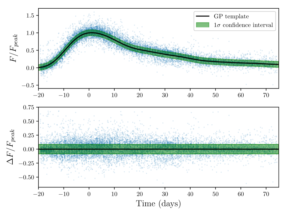
Figure 5: GP template of the combined light curves of 265 PTF and iPTF SNe Ia in flux space. The solid line shows the most likely function and the shaded region shows the 1 $\sigma$ interval, as predicted by GP. The axes show the normalised fluxes, $F/F_{peak}$, vs time in days. The lower panel shows the residuals, $\Delta F/F_{peak}$, of the template.

Reliability of the template

We test the robustness of our GP template by using Monte-Carlo simulations of the light curves with random Gaussian noise proportional to the measurement error and then repeating this for light curves with the same error and a systematic offset. To get an estimate on how sensitive all the parameters, such as stretch, time of maximum and maximum magnitude, are for noise we assume that our GP template is the “truth" and then re-fitting the simulated light curves (with added Gaussian noise proportional to the measurement error). We found that our template is robust (i.e. the standard deviation of the stretch was 0.04 for the 10,000 simulations) and use our results of the later simulation as an estimate for the error in the light curve parameters.

3.3 Searching for multiple populations

We can thus trust the template and are able to examine the residuals in order to search for multiple populations. If such were found it would point to diversity in the SNe physics. To measure the intrinsic scatter around each epoch, we divide the template into time bins of 9 days and fit Gaussian Mixture models from scikit-learn version 0.19.1 (Pedregosa et al., 2011) to each bin. The aim was to see if one Gaussian or more explain the distribution of each epoch bin better.

To evaluate the significance of this result we used the Bayesian information criteria (BIC) from Schwarz (1978), defined in equation 6, where $N$ is the number of data points in the fit, $\mathcal{L}$ is the maximum likelihood and $k$ is the number of parameters in the model.

$$BIC\equiv-2\ln\mathcal{L}+k\ln N$$ (6)

As discussed in Liddle (2004), BIC tends to favour models with fewer parameters compared to the commonly used Akaike information criteria (AIC), which is why we choose BIC for the purpose of determining if there is more than one population in the supernova parameters such as stretch. The best model is the one with the lowest value of BIC and if the difference between values of BIC, $\Delta$BIC is larger than 6 it is considered that the model is favoured significantly (see e.g. Sollerman et al., 2009). Since we prefer to be conservative in declaring a potential multiple population detection we require, in addition to $\Delta BIC>6$, that the mean of the two distributions is at least 3 $\sigma$ from each other.

We find that all bins are significantly better fitted ($\Delta BIC>6$) with more than one Gaussian with very similar mean values. As already stated we do not interpret this as a sign of multiple populations but rather that the tails on both ends of each bin are not captured by a single Gaussian. The exception is the bin around 25-34 days with respect to peak which shows 3 Gaussians for the best fit which do not share the same mean value. Thus we find no evidence for a pre-explosion outburst in days -30 to -15 wrt. maximum light but evidence for populations around the secondary maximum in the R-band.

We also searched for several populations in the light curve stretch distribution. Again, we used Gaussian mixture models and examined if the fit is improved compared to a single Gaussian fit.

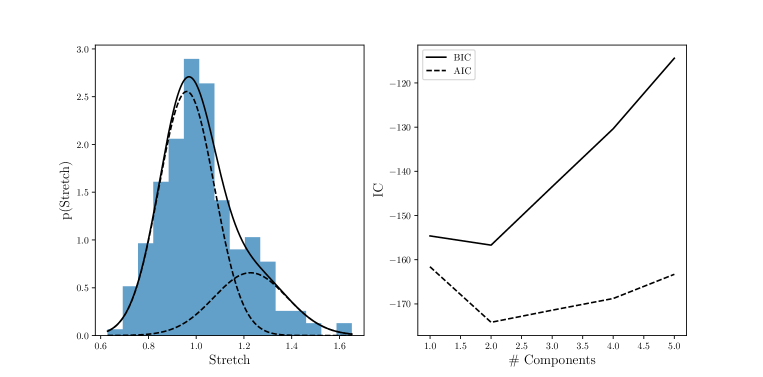
Figure 6: The left panel shows the combined mixture model in a solid line and two individual components in dashed lines. The right panel shows the information criteria (IC): AIC and BIC for different number of Gaussian components. The Gaussian Mixture model fit of the stretch distribution, where we see that both BIC, in the solid line, and AIC, in dashed line, favours two components over one.

Figure 6 shows the stretch distribution and the Gaussian mixture model fits, where we find that two Gaussian fit better than one ($\Delta BIC=2$). We thus conclude that there is no significant evidence for two populations over one. There are many examples in the literature of populations and asymmetry in stretch and colour (e.g. Jha et al., 2006; Mandel et al., 2009; Mandel et al., 2011; Li et al., 2011; Kessler et al., 2015; Ashall et al., 2016; Scolnic & Kessler, 2016).

3.4 Brightness evolution with redshift

By performing a two-sided Kolmogorov-Smirnov (KS) test on the “pull distribution", i.e., the error-weighted distribution of estimators around the true value on the binned light curves of different redshifts (seen in Figure 3), we find that the p-values are in many cases lower than 1%, i.e., we find no significant evidence for evolution in the light curve with redshift at any epoch. If the p-value is zero, it means that we cannot exclude the possibility that the distributions are different. This conclusion holds independent of the choice of bins.

4 Characterizing the light curve properties

In the next Section we use the unique history of upper limits before the supernova explodes to examine if there are any pre-explosion eruptions or post-explosion flares. Finding a pre-explosion eruption could give information about the progenitor of type Ia SNe. We are able to set limits for such an explosion but do not have the depth to exclude pre-explosion eruptions at the brightness level of a classic nova. We will also examine the average light curve parameters and look for multiple populations within the rise times.

4.1 Pre- and post- explosion limits

Since our dataset spans many days before and after explosion it is possible to look for pre- and post-explosion eruptions or bumps, similar to novae, which in turn would give us information about the progenitor of SN Ia and possible interaction with the environment of the SN. This was done for type IIn SNe in Ofek et al. (2014). By comparing the history of all individual light curves we looked for bumps before -30 days, and after +200 days with respect to maximum light. We used only the limits that were 20 magnitudes or deeper in this analysis. We do not find any significant perturbations before or after the supernova light is visible.

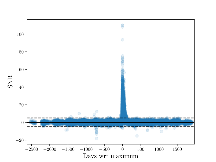
Figure 7: Signal-to-noise (SNR) distribution as a function of time from light curve peak of the fluxes of the SNe of our sample. The dashed lines show the 5 $\sigma$ limits. As discussed in the text the deviating data points (that are not part of the light curve, from day -20 to +100) come from various SNe and are not significant.

This might not be surprising since we do not have the sensitivity to detect bumps corresponding to the brightest observed novae, even for the most-nearby SNe in our sample. In Figure 7, we show the signal-to-noise ratio of our data points with respect to time of maximum (t=0 in the plot). We are not sensitive to novae since their absolute magnitude range is between $-10$ to $-5$ mag, as shown in Kasliwal (2011). We report that no eruption brighter than about $-15$ absolute R-band magnitude was found. The deepest limits come from the nearby supernova SN 2014J (iPTF14jj, see Goobar et al., 2014), showing the strength of nearby supernovae for this type of search.

Note that the detections in Figure 7, outside of the SN region, are not consecutive and thus considered in this analysis as noise. There are a variety of possible explanations for these detections including astrometric errors, cosmic rays, CCD ghosts, variable cloud coverage, other artefacts, unknown asteroids, etc. Zackay et al. (2016) showed that the classical method for image subtraction underestimates the noise due to several reasons (e.g., astrometric noise, source noise, correlated noise, reference image noise), and are less sensitive to cosmic rays (see example in Ofek et al., 2016).

We therefore set the criteria to require at least 2 consecutive detections in order to further examine if this is due to a pre-explosion eruption. In one case, iPTF13ccm, we observe two consecutive pre-explosion detections at -1000 days with respect to maximum light. This supernova is located near a bright star and thus these detections need to be confirmed. Therefore we run this supernova through an additional photometric pipeline but found that the images were of poor quality and could not confirm a pre-explosion detection. We therefore choose not to trust this pre-explosion detection.

A deeper survey such as the Large Synoptic Survey Telescope, (LSST Ivezic et al., 2008), would be needed to set more stringent limits on pre-explosion eruptions. We note in addition, that we find no post-explosion eruptions in our data.

4.2 Early light curves

The PTF and iPTF sample is unique in that it discovers supernovae very early, compared to other surveys. Comparing the first detection point, $p_{\rm first}$ in our sample with the low redshift literature supernovae from the JLA sample (Betoule et al., 2014), we find that the mean changes from $-12\pm 3$ to $-4\pm 5$ days. This is also illustrated in Figure 8. The PTF and iPTF sample have data points much earlier on average than the low redshift JLA sample and is therefore well suited for studies of the early part of the light curves.

Since the 1980’s there have been many studies of the early light curves of type Ia SNe. These studies found a correlation between the rise-time of a supernova and its brightness at maximum light, a shorter rise-time corresponding to a less luminous peak brightness.

While the early studies, (e.g Pskovskii, 1984; Phillips, 1993; Perlmutter et al., 1997) were only able to investigate this correlation, later studies with larger and more frequently sampled datasets (e.g. Conley et al., 2006; Strovink, 2007; Hayden et al., 2010; Ganeshalingam et al., 2011; González-Gaitán et al., 2012; Firth et al., 2015) looked in addition at the parametrisation and shape of the rise.

Kasen (2010) showed that if SNe Ia originate from a single degenerate scenario, i.e. with a giant companion, in about 10% of the cases there would be observational evidence of this in the early light curve in the form of an excess of flux. Hayden et al. (2010) and Ganeshalingam et al. (2011) found, in their studies of 108 and 61 supernovae light curves respectively, no evidence of interaction with a companion star. While they looked at the stacked light curves we will here examine each light curve individually and parametrise its rise-time and explosion time and then examine the average properties.

We used the analytical equation presented in Zheng & Filippenko (2017) to fit our supernovae light curve data to more easily be able to compare our results with literature values instead of using the Gaussian-processes template only. This analytic expression is derived from the photospheric-velocity-evolution function and makes the assumption that the emission is photospheric. It differs from the previous fitting methods by being less sensitive to where there is data in the light curve, (e.g., compared to Firth et al., 2015, which we found to not be robust for the majority of the light curves in our data set). We show the results of fitting the analytical equation to our data in Section 4.2.

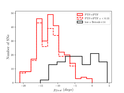
Figure 8: Histogram of earliest detection point, $p_{first}$ in days of our data sample from PTF/iPTF, compared with the low redshift sample from Betoule et al. (2014).

Now, looking at the individual light curves instead of the sample as a whole we chose to use the empirical equation from Zheng & Filippenko (2017), shown in equation 7 to fit our light curves in order to obtain parameters, primarily from the early time of the light curve. As mentioned earlier this part of the light curve is potentially important to probe the explosion mechanism and to distinguish between different progenitor scenarios. As opposed to most other empirical fits this equation fits the entire light curve and uses all available data, removing the need to cut at an arbitrary flux level before maximum light such as that used by Firth et al. (2015). The light-curve fits based on Zheng & Filippenko (2017), SALT2 (Guy et al., 2007) and the GP template yield very comparable results, as discussed in Appendix D.

The parameters in the equation are the normalising factor $A^{\prime}$, the explosion time $t_{0}$, the break time $t_{b}$, two free parameters determining the shape of the light curve, $\alpha_{r}$, $\alpha_{d}$ and a smoothing parameter $s$.

$$L=A^{\prime}\left[\frac{t-t_{0}}{t_{b}}\right]^{\alpha_{r}}\left[1+\left(\frac{t-t_{0}}{t_{b}}\right)^{s\alpha_{d}}\right]^{\frac{-2}{s}}$$ (7)

As suggested by Zheng & Filippenko (2017), we fix the values of $t_{b}=20.4$ days. We note considerable degeneracies between several other of the fitted parameters, especially between $t_{0}$, $\alpha_{d}$ and $\alpha_{r}$. The degeneracy is stronger in the cases where data around the rise time is sparse. We show in Figure 9 the combined limits for all SNe fitted, in total 207, since not all the SNe in the sample have sufficient data points before maximum light to get a good fit, keeping one of the parameters ($t_{0}$, $\alpha_{d}$ and $\alpha_{r}$) fixed at a time. We find the best fit values to be $-16.8^{+0.5}_{-0.6}$ days, $1.97_{-0.07}^{+0.05}$ and $2.36_{-0.03}^{+0.05}$ for $t_{0}$, $\alpha_{d}$ and $\alpha_{r}$ respectively, where the errors stated are the 1 $\sigma$ contours for each respective parameter. The value of the equivalent of $\alpha_{r}$ can be compared to the other studies which find a value between $\approx 1-3$ (e.g. Conley et al., 2006; Ganeshalingam et al., 2011; Firth et al., 2015; Zheng & Filippenko, 2017; Zheng et al., 2017) and while it is comparable with other surveys it is higher than expected from a fireball model where $\alpha_{r}=2$. We encourage testing different models for this early light curve data.

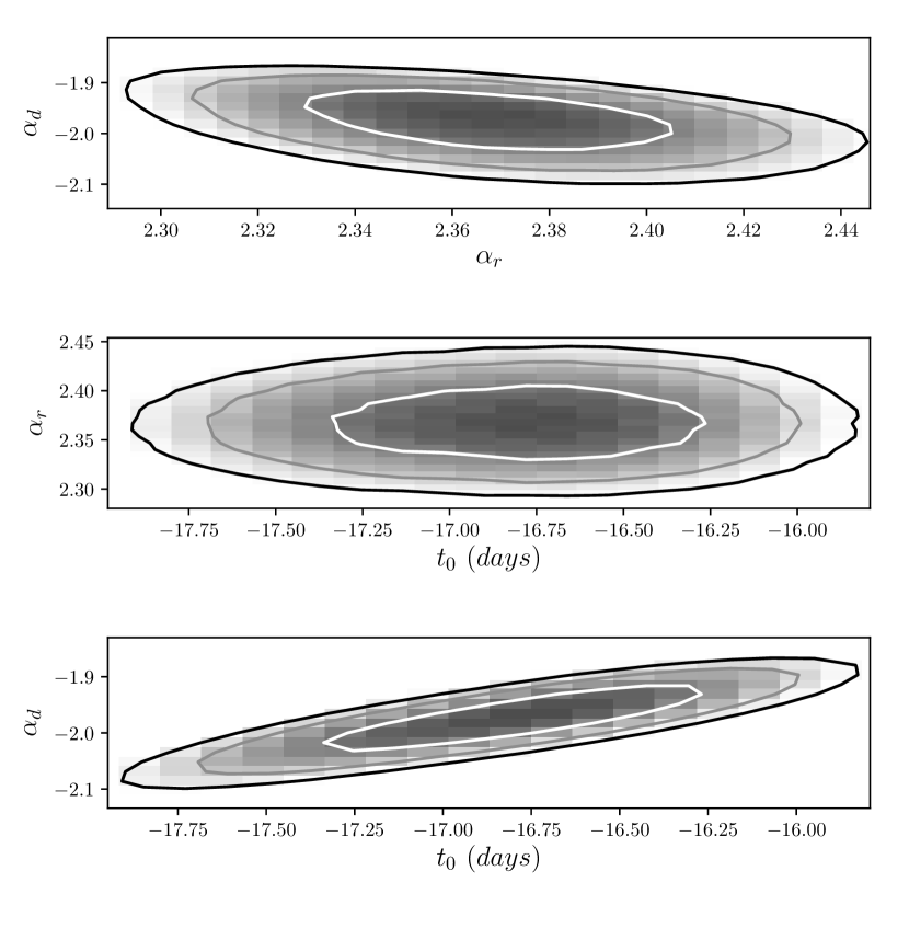
Figure 9: These three panels show the best fit values of equation 7 to 207 of the SNe in our sample. Because of the degeneracy between the parameters $t_{0}$ (in days), $\alpha_{d}$ and $\alpha_{r}$ we keep in one of these parameters fixed while the other two are free. The contour lines show 1,2 and 3 $\sigma$ confidence intervals for the sample.

4.3 Multiple populations in the rise-time

As with the stretch distribution we examined the possibility of multiple populations in the fitting parameters of equation 7. We perform Gaussian Mixture models (GMM) on a bootstrapped sample of our data where $\alpha_{d}$ is kept fixed and search for evidence of multiple populations in the $t_{0}-\alpha_{r}$ parameter space and find no statistically significant evidence for several populations. We note that the location of the minimum of each individual SN ellipse is widespread but with large errors. Due to these large errors Gaussian Mixture models cannot be used to distinguish possible multiple populations in the data. 49% of our 1000 bootstrapped samples showed one component fit the data significantly better (with $BIC>6$), 29% showed 2 components were a better fit and the rest were best fitted with more than 2 Gaussian components. We used the Bayesian information criterion since it sets more stringent restrictions and thus is more suitable to determine if there are more than one population in the data.

See Figure 10 for the histograms of the parameters. Note the spike at $t_{0}\approx-30$ days in the right panel of Figure 10 which is driven by SNe with insufficient data points in the early part of the light curve. As seen in the table LABEL:table:fitval in appendix 3 many of the best fit parameters have large errors. The fits to the light-curves and their $\chi^{2}$ can be found in the Supplementary materials. We do not interpret this spike as a hint of a second population, but rather problems with the fitting degeneracy. If more than one population was found this would have pointed towards more than one sub-population of SNe with different progenitor origins.

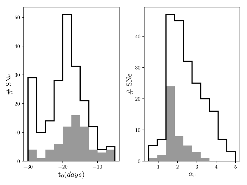
Figure 10: The histograms of the distributions of the best fit values of the $t_{0}$ and $\alpha_{r}$ parameters vs number of SNe. The peak at $t_{0}\approx-30$ days is driven by SNe with insufficient data points in the early part of the light curve and the error ellipses on these values are sometimes very large, for more details see in the text. The shaded regions show the fits with errors in $t_{0}<2$ days and $\alpha_{r}<0.2$.

5 Examining the Hubble-Lemaître residuals

Using the template as described in Section 3 we get the time of maximum estimate in the R-band for our sample with an accuracy of $\sim$ 1 day. The peak magnitude is then plotted against redshift in a Hubble-Lemaître diagram and shown in Figure 11. The rms of the Hubble-Lemaître residuals is 0.35 magnitudes for all redshifts after stretch corrections. In section 5.2 we discuss our estimate of the uncertainty stemming from not being able to correct for extinction. Figure 13 shows that this can be quite large, with a tail reaching $>0.5$ mag.

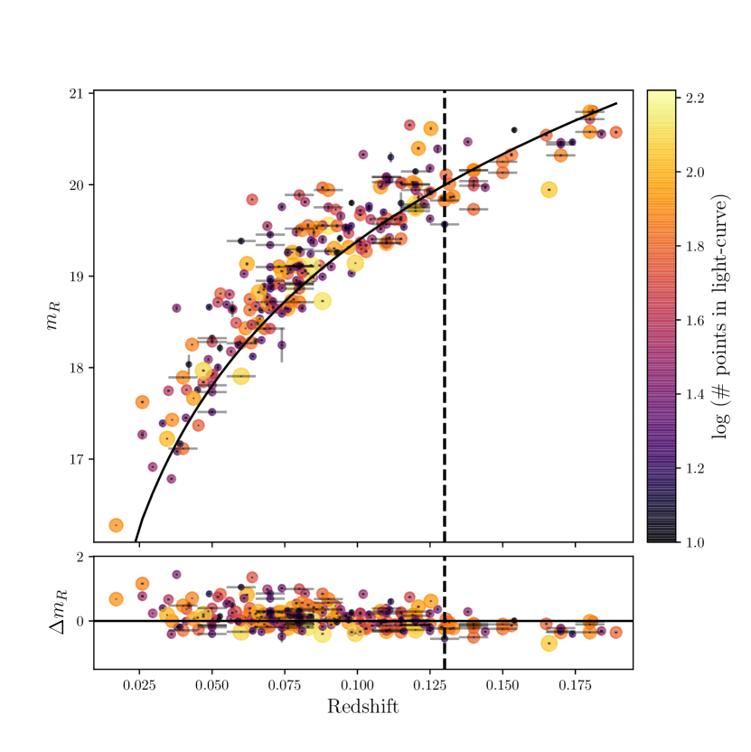
Figure 11: In the top panel we show the Hubble-Lemaître diagram, where the size of the data points are scaled logarithmically according to the number of data points that their light curves contain. The solid line shows the standard $\Lambda$CDM cosmology. The Hubble-Lemaître residuals for the sample are shown in the lower panel, with the dashed line indicating the redshift at which Malmquist bias becomes important. We do not include the outlier supernova SN2014J, since this supernova is highly reddened and very nearby. As discussed in the text, these SNe are not corrected for extinction.

5.1 Malmquist bias

An important systematic for type Ia SN cosmology is Malmquist bias (Malmquist, 1922), which is the redshift on beyond which the survey becomes flux limited, i.e. when we probe only the brightest SNe rather than the entire population. We determine at which redshift this bias becomes important for our sample in order to account for this and to plan future survey strategies for the Zwicky Transient Facility (ZTF). We thus need to estimate the underlying distribution of Hubble-Lemaître residuals. To do this, we fit the convolution of two functions, an exponential and a Gaussian to estimate the mode at different redshift bins.

To determine where the Malmquist bias becomes important we require a 3 $\sigma$ deviation in the Hubble-Lemaître residuals. This is found at both high and low redshifts. At low redshifts the mode is 3 $\sigma$ above zero due to peculiar velocities and highly extinct SNe at low redshift. At higher redshift, we can see that we get a 3.4 $\sigma$ deviation to the faint end at $z=0.13$. In Figure 11 the dashed line shows where this limit lies in the Hubble-Lemaître diagram and in Figure 12 we show the histogram of two bins, one of which is Malmquist biased. We thus determine that Malmquist bias becomes statistically significant at redshift 0.13 for our sample.

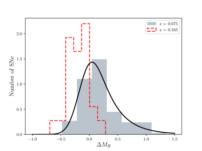
Figure 12: We show the distribution of Hubble-Lemaître residuals for two different redshift bins centred around 0.075 and 0.165 in shaded grey and the dashed line respectively. The solid black line shows the best fit convolution between a Gaussian and an exponential used to determine the mode of the histograms of Hubble-Lemaître residuals in order to estimate where the Malmquist bias becomes important.

5.2 Average extinction and mean dust path

One of the largest systematic of type Ia SNe is the extinction by dust. This can be corrected for using the colour-magnitude correlation found in literature.

Since our sample does not have additional filter information, this correction could not be performed for individual SNe, however we were able to estimate the average path length of dust that the SN light travelled through for our sample. This can then be translated into an average extinction of all SNe in our sample to correct the maximum magnitude of R-band SNe.

To understand the origin of the Hubble-Lemaître residual distribution we use the SuperNova Observation Calculator (SNOC, described in Goobar et al., 2002), to create simulated supernova samples with different amounts of extinction. We use the code to generate samples of $2000$ type Ia SNe using the same redshift distribution we have from our iPTF and PTF sample.

For each iteration we change two parameters; the intrinsic scatter (characterised by the width of the Gaussian part in fitting the Gaussian convoluted with an exponential as we did to determine the Malmquist bias) and the mean free path for host galaxy dust extinction. We allow the values to vary from $0.1-0.30$ magnitudes and $1\times 10^{-5}-1\times 10^{-2}$ Mpc for intrinsic scatter and host dust extinction respectively. We then compare the Hubble-Lemaître residual distribution from each $SNOC$ iteration with our own sample distribution using a double-sided K-S test.

We find the minimum to lie at 1 kpc corresponding to a mean $E(B-V)$ of $\approx 0.05(2)$ magnitude or an $A_{R}\approx 0.11$ magnitude, assuming $R_{V}=3.1$.

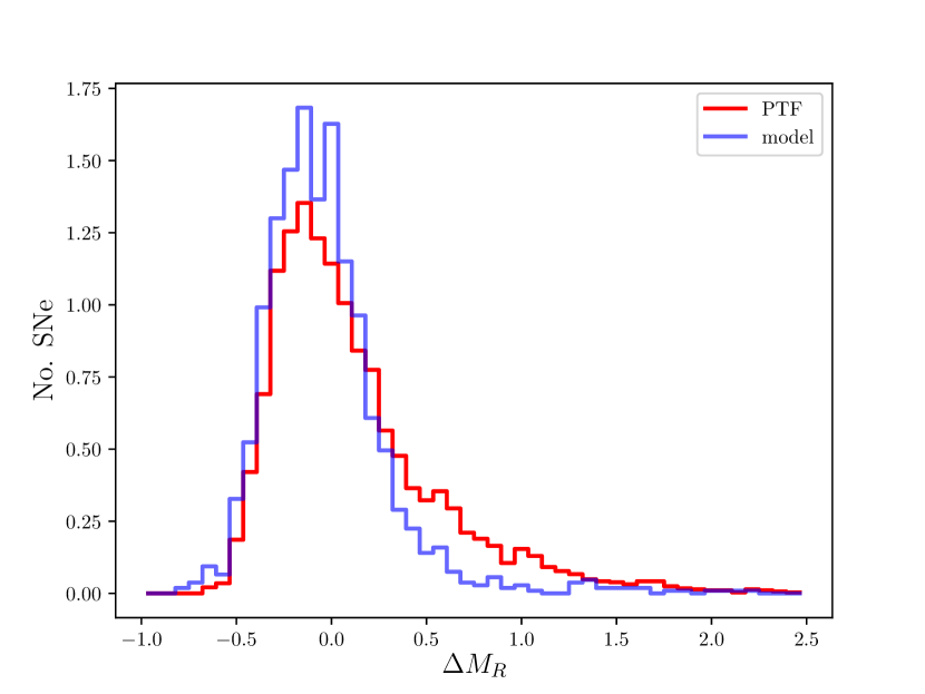
Figure 13: An example plot of the normalised Hubble-Lemaître residuals, $\Delta M_{R}$ where the SNOC model is consistent with our distribution. The red curve shows the PTF and iPTF Hubble-Lemaître residual distribution and the blue curve the model with a mean free path of $1$ kpc and an intrinsic scatter of $0.2$ magnitudes. The plot is normalised so that the area under each curve equals 1.

While the double sided K-S test does not give a confidence interval the results are consistent with an average mean free path of $10^{-3}$ Mpc. An example where the model is consistent with the Hubble-Lemaître residuals in our sample is shown in Figure 13. It is important to note that the SNOC simulations are idealised and treat measurement errors in a simplified way, thus we do not get a very good fit to our data. We do not reach a clear minimum for the intrinsic scatter parameter. By visual examination of the fits the negative Hubble-Lemaître residuals are overestimated for high values of intrinsic scatter in the model, yet yield a lower K-S statistic. While this means that we cannot constrain the intrinsic scatter using this method, the common minimum at $1$ kpc for all values of the intrinsic scatter suggests that the average mean free path we get is consistent with our data. The intrinsic scatter is thus constrained using the Gaussian part of the fit to the convolution of a Gaussian and an exponential (which was also used to obtain the Malmquist bias) and is found to be $0.186\pm 0.033$ magnitudes for the redshift range 0.05 to 0.1.

From these results we have a better understanding of the average bias that our Hubble-Lemaître residuals have since they have not been corrected for colour.

We attempted to use the low-resolution spectra taken to classify the SNe (at least one per supernova) to get an estimate of the amount of extinction. However synthetic colours do not show any correlation with Hubble-Lemaître residuals and thus cannot be used to correct for extinction. This is thought to be due to the uneven flux calibration performed on these spectra. This was also noted by Maguire et al. (2014) for the PTF spectra. Note that we do not correct for gravitational lensing of objects in the line of sight in the simulations. This effect is negligible at the these low redshifts.

5.3 Mass step in SN hosts

The aim is to examine the correlation between the host mass and Hubble-Lemaître residuals found in several papers with varying degrees of significance on the slope in the B-band (e.g. Lampeitl et al., 2010; Sullivan et al., 2010; Childress et al., 2013; Wolf et al., 2016; Pan et al., 2014; Kelly et al., 2010; Scolnic et al., 2017; Jones et al., 2018; Rigault et al., 2018).

We show in Figure 14 the Hubble-Lemaître residuals in the R-band from our sample with $z<0.13$ and the log mass of the host galaxies from Hangard et al. (in prep.).

Hosts stellar masses are calculated using FAST (Fitting and Assessment of Synthetic Templates Kriek et al., 2009), a code that fits stellar population templates to photometry. We use $ugriz$ magnitudes from SDSS (Alam et al., 2015) and $JHK_{s}$ magnitudes from 2MASS (Skrutskie et al., 2006). Each host must have a known redshift, and at least 2 data points in magnitudes. Only photometry with errors smaller than 0.25 magnitudes are considered. The stellar populations library used is FSPS by Conroy & Gunn (2010), and the star formation history is chosen delayed, exponentially declining. The initial mass function is from Chabrier (2003), and the dust law is from Kriek & Conroy (2013). The metallicity is fixed to solar metallicity value (Z = 0.019). We only keep the fits for which the reduced $\chi^{2}$ is smaller than 2.

We find the Hubble-Lemaître residual step is $0.037\pm 0.068$ is compatible with the latest results from Scolnic et al. (2018). However, our results is also compatible with no step in the Hubble-Lemaître residuals. We found no redshift dependence on the mass step measurement for $z\leq 0.13$, which is why we restricted the SNe to that redshift range, coinciding with our adopted estimate of the onset of a significant Malmquist bias, see section 5.1.

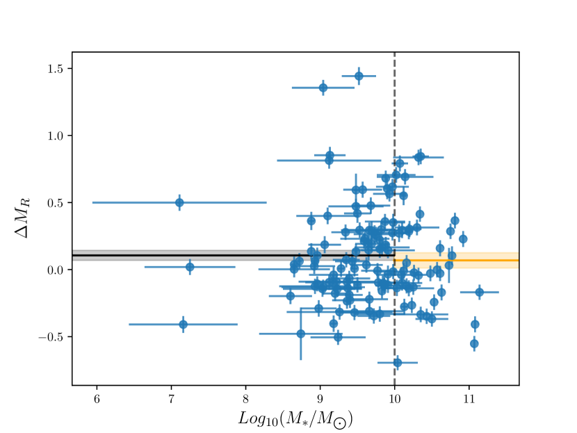
Figure 14: We are showing the Hubble-Lemaître residuals in R-band, $\Delta M_{R}$ vs. the log of the host stellar mass, $\rm log_{10}M_{\ast}/M_{\bigodot}$, for 131 of the SNe in our sample that have reliable host masses. We include K-correction, calibration, photometric and peculiar velocity errors in the Hubble-Lemaître residual error-bars. The dashed line shows the definition of high and low mass host galaxy (see e.g. Sullivan et al., 2010, 2011), and the horizontal lines with the shaded areas show the mean and standard error for each of the two host mass bins.

6 Discussion

We presented the light curve analysis from PTF and iPTF, an un-targeted survey which addresses one of the main problems in present day cosmology with type Ia SNe; namely the sampling bias. However, since we do not address another significant bias, the colour of the SNe, we have focused this paper on looking at the average light curve properties.

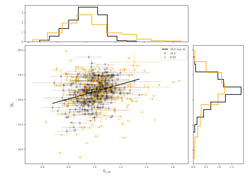
Figure 15: Showing the peak absolute magnitude, $M_{r}$ vs. stretch, $S_{r}/R$ relation for the JLA nearby supernova sample, Betoule et al. (2014), in the SDDS r-band in black circles and the PTF and iPTF sample in orange. We also show the best fit line the JLA sample, showing the weak but significant correlation between the parameters. For the PTF sample this correlation is weaker. Note that we have performed an offset corresponding to the S-correction, Stritzinger et al. (2005), of 0.35 magnitudes between the two different filter bands.

A commonly used way to reduce the Hubble-Lemaître residuals is to use the relation between the peak brightness and the width of the light curve, such as stretch (Perlmutter et al., 1997). In order to compare with literature on r-band only fits we used sncosmo to calculate the absolute magnitudes and stretch of the JLA low redshift supernova sample from Betoule et al. (2014) using the template from Hsiao et al. (2007). The results for the fits based exclusively on the SDSS r-band are shown in Figure (15). To estimate the significance of the correlation between the two parameters $S_{R}$ and $M_{r}$ we use Spearman R statistic and bootstrap the data-points according to their individual errorbars and covariance between the two parameters. We do this 10 000 times and find that the average Spearman $R=0.2$ with $p-value<10^{-7}$. For the PTF sample the correlation is weaker. If we now compare the slope of this with that of the B-band from Burns et al. (2011) (with $\Delta m_{15B}$) with a value of $0.58\pm 0.10$ we see that the slope is less steep in the redder band. This could be due to the relative flatness of the R-band light curve compared to other photometric bands. We also note that, after having performed an S-correction of 0.35 magnitudes, the calibration the PTF and iPTF SNe are consistent with that of the low redshift JLA sample.

While we in this work look at the average properties of type Ia SNe from an untargeted survey we do not take other biases into account. To improve the quality of this data sample there are a number of things that can be done. Perhaps the most important is to have colour information for each SN such that extinction can be corrected for on an individual SNe level. Secondly, a better calibration of the photometry would be very beneficial. Both these changes are being applied to the ZTF, (Bellm, 2014) type Ia SNe survey as well as expanding the data sample. ZTF came online in February 2018 (Kulkarni, 2018) and will be 15 times more efficient than iPTF. With a substantially larger field of view of 47 deg², faster reading and slewing speed it is expected to be able to find 15 times the amount of transient events, including many SNe Ia. Other future surveys of importance for SN Ia discovery and follow-up include the LSST (Ivezic et al., 2008) which is scheduled to be operational in 2022.

7 Conclusion

We present in this paper the best 265 sampled SNe type Ia from homogeneous PTF and iPTF dataset in order to examine the light curve properties in the Mould R band of a non-targeted survey. The full tables are in Appendix 3 with both the values from the R-band light curve and the individual parameters from the fit of equation 7 from Zheng & Filippenko (2017). All individual light curve photometry used in this paper is made publicly available through WISeREP, (Yaron & Gal-Yam, 2012).

Our conclusions can be summarised as follows:

• We constructed and present a non-parametric template of our sample SNe spanning between -20 and +80 days with respect to maximum light. Since this was constructed with the help of heteroscedastic Gaussian processes we can provide a 90% confidence region around the template that takes the errors of each data point into account. We used this to examine the intrinsic scatter and found no evidence for multiple populations at any bin along the template. We note a wider spread around the time of the light curve shoulder, $\approx 30$ days after peak.

• We determined the Malmquist bias in our sample to become noticeable at $z=0.13$ by fitting a Gaussian and an exponential to the Hubble-Lemaître residuals.

• Since this survey was made in one band we cannot correct for individual SNe extinction. We thus determine the average extinction to be E(B-V) $\approx 0.05(2)$ magnitudes or $A_{R}=0.11$ magnitudes and the average mean free path for dust extinction to be $10^{-3}$ Mpc by comparing to simulations with SNOC.

• We find no redshift evolution in the light curve at any epoch in our sample, when dividing into 3 redshift bins, up to z=0.2.

• We search for pre- and post- explosion flares in our data spanning from -2500 days to +2000 days with respect to maximum and find no significant flare. We note that nearby SNe are especially useful in setting these limits and that the PTF/iPTF depth is not enough to reach the brightness of a novae.

• We used the analytical equation presented in Zheng & Filippenko (2017), equation 7 and fit to 200 of our light curves and get a rise time and rise index for each SN. We then look at the average properties of these and found the best fit values to be $-16.8^{+0.5}_{-0.6}$ days, $1.97_{-0.07}^{+0.05}$ and $2.36_{-0.03}^{+0.05}$ for $t_{0}$, $\alpha_{d}$ and $\alpha_{r}$ respectively, where the errors shown are the larger 1 $\sigma$ contours from the contour ellipses of the parameter fits.

• We searched for multiple populations using Gaussian mixture models in individual bins around the Gaussian processes template of the light curves, stretch and rise times as measured with equation 7. We did not find significant evidence of more than one population in any of these parameters.

• We find that the Hubble-Lemaître residual step is $0.037\pm 0.068$ which is both compatible with a zero slope and literature values. We conclude that our data is not sensitive enough to probe the host mass -luminosity relation.

Appendix A Photometric filter

In Figure 16 we show how the R-band filter used for our data sample compares with other filters more commonly used in the literature, such as the Bessel R and SDSS r, see Bessell (2005) for a review of different filters. The latter was used in Betoule et al. (2014) to which we compare our sample in Section 6.

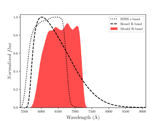
Figure 16: This plot shows a comparison between different filter functions used, we show the Mould R-band used in this paper for our data analysis, the Bessel R and the SDSS r filter.

Appendix B Forced Photometry and magnitudes in our dataset

B.1 Baseline correction

We have used forced photometry in our analysis which is performed with difference imaging of the data and gives a relative photometry. We then convert this to an absolute photometry as described in Section B.4. Before that conversion we make a baseline correction to the initial light curve to correct for any residual offset in the “history" of the light curve. We choose to define any point earlier than 50 days before peak to be defined as “history" and use these points to determine the level of this baseline. The baseline correction is necessary to account for when the reference image was taken. If the reference image includes SN flux or includes a different systematic the photometry will not be correct without this correction. In the light curves accompanying this paper there is a flag for when this baseline correction could not be performed due to lack of sufficient “historical" data points.

B.2 Quality checks

We perform two checks to ensure that the photometry can be trusted.

• We compare the point spread function (PSF) photometry to aperture photometry to see if there is any global bias for positive flux measurements and to detect global systematics in the PSF-templates since aperture photometry is less affected by astrometric error.

• We only use photometry with PSF sharpness (a parameter given by the pipeline) of $\approx 1$ indicating a PSF-like source rather than a spike or extended profile.

B.3 Uncertainties in the photometry

We calculate the uncertainties in the fluxes by multiplying the 1 $\sigma$ uncertainties in the PSF-fit fluxes with a scaling factor as shown in equation 8.

$$\sigma_{F(\rm corrected)}=scaling\hskip 2.84526ptfactor\times\sigma{F(\rm raw)}$$ (8)

The scaling factor is defined as the division of the standard deviation and the median of the “historic" flux, $F(t_{i},t_{f})$ as shown in equation 9.

$$scaling\hskip 2.84526ptfactor=\sigma_{F(t_{i},t_{f})}\hskip 2.84526pt/<F(t_{i},t_{f})>$$ (9)

This way of calculating the uncertainties assumes that there is no transient light in the “historical" part of the light curve.

B.4 Absolute photometry

We then convert the relative photometry to absolute photometry by using the zero point extracted from the reference-image SExtractor catalogue (Bertin & Arnouts, 1996) for stars between the R-band magnitude, $14.5\leq m_{R}\leq 19.0$ using aperture photometry. If the zero point was not possible to get for a particular image we used the median zero point from the rest of the measurements for the same object. All measurements with a signal-to-noise of more than 3 are classified as detections and thus their magnitude is found with equation 10,

$$M=ZP-2.5\log(F(\rm corrected))$$ (10)

otherwise we report them as limits following equation 11.

$$M_{limit}=ZP-2.5\log(3*\sigma_{F(\rm corrected)})$$ (11)

Appendix C Gaussian processes in machine learning applied to SN light curves

Gaussian processes is a machine learning algorithm for non-parametric regression, i.e. it allows reconstruction of a function without assuming parametrisation or functional form. For a more complete overview of Gaussian processes, see Rasmussen & Williams (2005). We are looking for the latent function (i.e. the true function) $f(t)$ that maximises the likelihood of producing the observed data under the assumption of independent Gaussian noise. Gaussian Processes approximates the latent function as

$$GP(m(t),k(t,t^{\prime}))\approx f(t),$$ (12)

given the expected mean, $m(t)$, and a covariance function or kernel, $k(t,t^{\prime})$, defined to be:

$$m(t) =\mathbb{E}\left[f(t)\right]$$ (13)

$$k(t,t^{\prime}) =\mathbb{E}\left[(f(t)-m(t))(f(t^{\prime})-m(t^{\prime}))\right].$$ (14)

where $\mathbb{E}$ denotes the expectation value.

The kernel is a measure of similarity between two points, which can be defined as a distance between two functions $f$ and $g$ as:

$$d(f,g)={f|k|g}=\int_{\mathcal{R}}f(t)k(t,t^{\prime})g(t^{\prime})dtdt^{\prime}.$$ (15)

One of the most commonly used kernels is the squared exponential (also called Radial basis function, $RBF$) defined in equation 16, where $\sigma$ is the noise of the data and $l$ the length scale of the kernel.

$$k(t,t^{\prime})=\sigma^{2}\hskip 2.84526pte^{-\left(\frac{(t-t^{\prime})^{2}}{2l^{2}}\right)}$$ (16)

The length scale defines the distance between points at which correlation between them is lost. In other words if points are much further away from each other than the length scale they become irrelevant. This kernel depends on two hyper-parameters, $\sigma$ and $l$ that have to be set (see Section (C.1)).

C.1 Model Section of kernels

The likelihood of obtaining the vector of $N$ observations $\underline{\mathbf{y}}=[y_{1},y_{2}...y_{N}]$ at points $\underline{\mathbf{T}}=[t_{1},t_{2}...t_{N}]$ given a kernel of hyper-parameters $\underline{\boldsymbol{\theta}}$ (in our squared exponential example, $\underline{\boldsymbol{\theta}}=[\sigma,l]$) is given by:

$$\log p(\underline{\mathbf{y}}|\underline{\mathbf{T}},\underline{\boldsymbol{\theta}})=-\frac{1}{2}\underline{\mathbf{y}}^{T}K^{-1}\underline{\mathbf{y}}-\frac{1}{2}\log|K|-\frac{N}{2}\log 2\pi$$ (17)

where the covariance matrix, $K_{ij}=k(t_{i},t_{j})$ containing the pair-wise distances between data points. The first term of equation 17 measures the goodness of the fit, the second is a complexity penalty and the third is a normalisation.

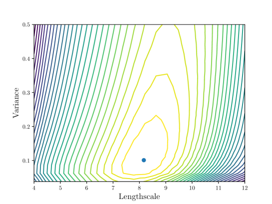
Figure 17: A contour plot of the log likelihood as a function of length-scale and variance hyper-parameters of the kernel for a light curve from our sample, iPTF13asv. The dot marks the optimal choice of hyper-parameters.

The gradients of equation (17) with respect to the hyper-parameters can be computed analytically; so we can efficiently compute the hyper-parameters that maximise the likelihood. This is shown in Figure 17 using an example light curve from our data set. As seen in the Figure the chosen hyper-parameters lie at the maximum log likelihood. Since the contours of variance and length scale only have one maximum (in the case of our light curves) we do not need to perform cross-validation to obtain the best hyper-parameters. The most computationally expensive part is inverting the covariance matrix which requires a time $\mathcal{O}(N^{3})$, and is the limiting factor for performing GP on large datasets.

Once optimised, we can choose between different kernels by choosing the one with greater likelihood.

C.2 Additional kernels

The square exponential kernel, shown in equation 16 forces the GP to be infinitely smooth, which may be unrealistic for some datasets. In our analysis we use the best kernel or a linear combination of different kernels used in the literature, to fit our data. The ones we use are introduced in the following Section. In Figure (18) we show an example of a light curve from our dataset under different kernels. Note that the biggest difference is when the data is sparse as shown in the inset-plot.

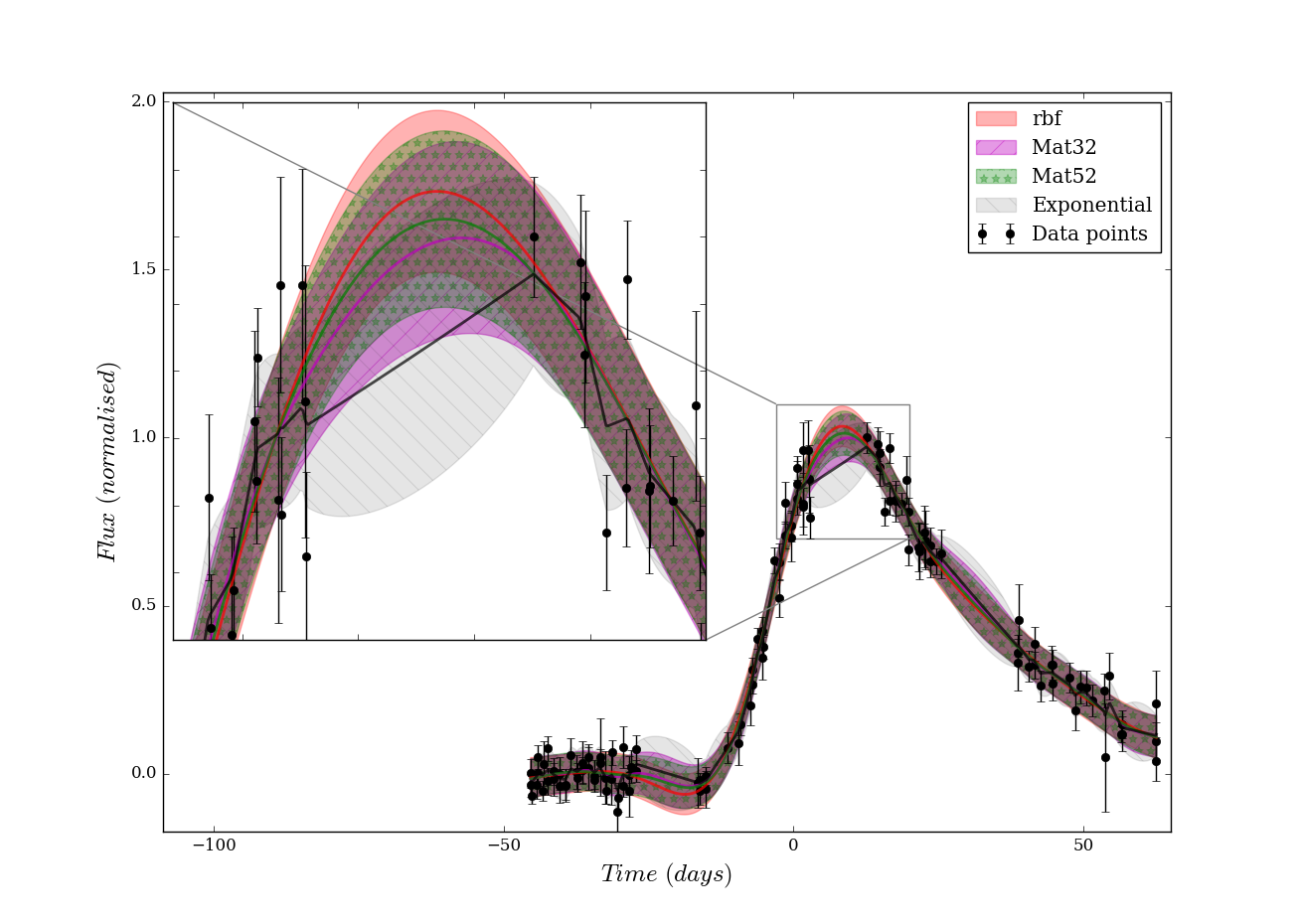
Figure 18: A plot of GP with different kernel for one of the supernovae light curves in our sample, iPTF13hpz. The solid lines (red, green, magenta and black for RBF, Matérn with $\nu=3/2$ and $\nu=5/2$ and the exponential kernel respectively) show the latent functions and the shaded areas the $1\sigma$ confidence interval. The zoomed in Section is the area near the maximum light where data points are missing.

C.3 The Matérn family

For a given $\nu$ the Matérn kernels is defined as:

$$k_{\nu}({\bf{t}},{\bf{t^{\prime}}})=\sigma^{2}\left(\frac{1}{\Gamma(\nu)2^{\nu-1}}\left[\frac{\sqrt{2\nu}}{l}|{\bf{t}}-{\bf{t^{\prime}}}|\right]^{\nu}K_{\nu}\left(\frac{\sqrt{2\nu}}{l}|{\bf{t}}-{\bf{t^{\prime}}}|\right)\right),$$ (18)

where $\nu$ regulates the smoothness of the function and is determined by how differentiable it is. $K_{\nu}$ is the modified Bessel function of second kind of order $\nu$, and $l$ is the characteristic length scale. From this family of kernels, we will select two cases of $\nu$:

$$k_{3/2}(t-t^{\prime})=\sigma^{2}\left(1+\frac{\sqrt{3}|t-t^{\prime}|}{l}\right)\exp\left(-\frac{\sqrt{3}|t-t^{\prime}|}{l}\right)$$ (19)

and

$$k_{5/2}(t-t^{\prime})=\sigma^{2}\left(1+\frac{\sqrt{5}|t-t^{\prime}|}{l}+\frac{5(t-t^{\prime})^{2}}{3l^{2}}\right)\exp\left(-\frac{\sqrt{5}|t-t^{\prime}|}{l}.\right)$$ (20)

Note that as $\nu\rightarrow\infty$ we recover the squared exponential.

C.4 Exponential kernel

If $\nu=\frac{1}{2}$ we get the exponential kernel and the resulting function is continuous but non-differentiable. In 1D this corresponds to the Ornstein-Uhlenbeck process, a model of Brownian motion. It is defined as:

$$k(t-t^{\prime})=\sigma^{2}\exp\left(-\frac{|t-t^{\prime}|}{l}\right).$$ (21)

C.5 White noise

To model a process that is not continuous we can use the white noise kernel,

$$\mathscr{W}=\sigma^{2}\delta(t-t^{\prime}),$$ (22)

where $\delta$ is Dirac’s $\delta$.

C.6 Linear kernel

Gaussian processes can also be reduced to a linear regression through the linear kernel,

$$k(t,t^{\prime})=\sigma^{2}+t\cdot t^{\prime}.$$ (23)

C.7 New kernels through linear combinations

We can also create new kernels by adding them in a linear combination. This can be used, for example, when both short scale and long scale phenomena are present in the data, which allows one kernel to have a different length-scale than the other. In particular we could use the linear kernel to capture the kernel to capture the global trend and the squared exponential to model local distortions. As mentioned in equation (17) there is a penalty for increased complexity preventing over-fitting.

C.8 Heteroscedastic Gaussian Processes

In its simplest formulation Gaussian Processes assumes that all the points have the same Gaussian noise and that this can be learned from the data. However in observational data we have known and different uncertainties. We can incorporate this by using a linear combination of kernels and a white noise kernel with $\sigma_{i}$ given by the uncertainties of the data:

$$\mathscr{W}=\left[\sum_{i}\sigma_{i}^{2}\delta(t-t_{i})\right]\delta(t-t^{\prime}),$$ (24)

Appendix D Model comparison

In this paper we have used three different methods to fit the R-band light-curves of PTF and iPTF; based on Zheng & Filippenko (2017), SALT2 (Guy et al., 2007) and the GP template. Here we compare how statistically similar the light-curve fits are. With respect to the goodness of fit: 81 %, 88 % and 100% of the fits for each method respectively have $\chi^{2}/{\rm ndof}<3$. The SALT2 fit values can be found Table LABEL:table:salt2 and the values from Zheng & Filippenko (2017) in Table LABEL:table:fitval. We note that the $\chi^{2}$ is calculated only where each of the respective models are defined which is different for the 3 models (Zheng & Filippenko (2017) is only fitted to before the secondary maximum at $+15$ days, SALT2 (Guy et al., 2007) until $+50$ days and the GP template until $+80$ days), which makes a direct comparison harder.

To further investigate the $\chi^{2}/{\rm ndof}$ differences between the models we compare the Pull distributions, i.e. the error weighted residuals. We first check whether they are consistent with a normal distribution for the three models, as seen in figure 19. We also compare the Pull distributions as a function of phase and see no significant difference between the models. This is done in order to ascertain that none of the models fails to capture significant features of the light-curve within their entire model range, which could skew the distribution and would show up as a phase dependence. Since the models perform similarly we use the Zheng & Filippenko (2017) model because its parameters are easier to interpret physically.

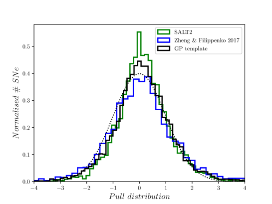
Figure 19: Here the Pull distributions, i.e. residuals/error is shown for the 3 different light-curve fitting methods used in this paper. The dotted line shows a Gaussian with $\sigma=1$, $\mu=0$ for comparison.

Appendix E Tables of light-curve parameters

Table 2: Best fit values for each supernova with their respective asymmetric errors.

PTF name	$t_{0}$ (days)	A’	$\alpha_{d}$	s	$\alpha_{r}$
10aaju	$-30.0_{-0.0}^{+3.527}$	$7.183_{-1.762}^{+1.209}$	$-6.085_{-0.226}^{+1.914}$	$0.529_{-0.028}^{+0.185}$	$2.695_{-0.138}^{+0.11}$
10aajv	$-30.0_{-0.0}^{+2.54}$	$31.952_{-4.062}^{+4.753}$	$-4.5_{-0.217}^{+0.393}$	$0.3_{-0.0}^{+0.008}$	$3.176_{-0.058}^{+0.061}$
10aayx	$-24.205_{-3.474}^{+1.535}$	$1.349_{-0.043}^{+0.524}$	$-1.506_{-0.74}^{+0.193}$	$3.0_{-1.305}^{+0.0}$	$1.573_{-0.06}^{+0.212}$
10abjm	$-30.0_{-0.0}^{+0.97}$	$9.614_{-1.175}^{+1.471}$	$-6.764_{-0.127}^{+0.657}$	$0.452_{-0.021}^{+0.041}$	$2.926_{-0.087}^{+0.095}$
10abou	$-19.359_{-9.88}^{+1.325}$	$1.54_{-0.058}^{+0.369}$	$-1.431_{-0.149}^{+0.16}$	$3.0_{-2.164}^{+0.0}$	$1.682_{-0.051}^{+0.169}$
10abws	$-22.145_{-7.855}^{+10.073}$	$2.939_{-1.467}^{+9.834}$	$-2.819_{-4.181}^{+1.5}$	$1.172_{-0.313}^{+1.777}$	$2.388_{-0.5}^{+0.91}$
10cko	$-27.36_{-2.122}^{+2.265}$	$62.147_{-17.079}^{+14.27}$	$-6.246_{-0.754}^{+0.713}$	$0.3_{-0.0}^{+0.018}$	$4.064_{-0.201}^{+0.108}$
10cmj	$-17.525_{-12.475}^{+5.017}$	$2.748_{-2.388}^{+17.567}$	$-1.816_{-4.225}^{+1.007}$	$1.291_{-0.841}^{+1.561}$	$2.053_{-0.46}^{+0.775}$
10czc	$-29.999_{-0.001}^{+6.147}$	$3.894_{-1.352}^{+1.122}$	$-6.799_{-0.201}^{+3.781}$	$0.602_{-0.046}^{+0.585}$	$2.274_{-0.165}^{+0.189}$
10feg	$-26.22_{-2.971}^{+3.466}$	$60.441_{-24.539}^{+20.138}$	$-5.986_{-1.014}^{+0.999}$	$0.3_{-0.0}^{+0.039}$	$3.891_{-0.285}^{+0.129}$
10fxl	$-13.0_{-0.676}^{+0.726}$	$15.588_{-7.065}^{+1.178}$	$-3.054_{-0.458}^{+0.326}$	$0.491_{-0.131}^{+0.136}$	$3.263_{-0.301}^{+0.45}$
10gjx	$-15.911_{-0.745}^{+0.992}$	$88.173_{-71.352}^{+2.003}$	$-3.654_{-0.2}^{+0.695}$	$0.3_{-2.697}^{+2.697}$	$3.917_{-0.672}^{+0.075}$
10glo	$-30.0_{-0.0}^{+5.601}$	$65.365_{-17.083}^{+18.315}$	$-5.501_{-0.159}^{+0.785}$	$0.3_{-0.0}^{+0.021}$	$3.632_{-0.148}^{+0.105}$
10goo	$-19.612_{-2.295}^{+2.155}$	$81.65_{-68.276}^{+2.362}$	$-3.656_{-0.398}^{+0.772}$	$0.3_{-2.533}^{+2.533}$	$3.582_{-0.734}^{+0.1}$
10gop	$-28.291_{-1.34}^{+1.787}$	$56.391_{-11.726}^{+11.476}$	$-6.568_{-0.432}^{+0.644}$	$0.3_{-0.0}^{+0.012}$	$4.163_{-0.174}^{+0.138}$
10goq	$-21.228_{-1.956}^{+3.797}$	$1.518_{-0.074}^{+0.089}$	$-1.571_{-0.406}^{+0.387}$	$3.0_{-0.349}^{+0.0}$	$1.483_{-0.078}^{+0.072}$
10hcu	$-13.403_{-0.335}^{+0.185}$	$1.16_{-0.035}^{+0.048}$	$-0.912_{-0.092}^{+0.083}$	$3.0_{-0.16}^{+0.0}$	$1.422_{-0.119}^{+0.128}$
10hdm	$-22.132_{-1.151}^{+1.336}$	$1.354_{-0.038}^{+0.052}$	$-1.758_{-0.184}^{+0.164}$	$3.0_{-0.249}^{+0.0}$	$1.301_{-0.066}^{+0.071}$
10hdn	$-30.0_{-0.0}^{+17.002}$	$7.473_{-6.043}^{+3.443}$	$-6.752_{-0.241}^{+0.246}$	$0.485_{-0.059}^{+0.058}$	$2.59_{-0.892}^{+0.258}$
10hei	$-19.82_{-1.044}^{+1.206}$	$1.362_{-0.039}^{+0.074}$	$-1.686_{-0.159}^{+0.151}$	$3.0_{-0.346}^{+0.0}$	$1.576_{-0.059}^{+0.062}$
10hne	$-18.327_{-1.603}^{+1.412}$	$87.897_{-81.376}^{+3.162}$	$-3.858_{-0.314}^{+1.267}$	$0.3_{-0.249}^{+0.249}$	$3.945_{-1.179}^{+0.119}$
10hpp	$-16.78_{-2.044}^{+2.944}$	$1.468_{-0.083}^{+0.175}$	$-1.426_{-0.216}^{+0.224}$	$3.0_{-0.61}^{+0.0}$	$1.582_{-0.081}^{+0.102}$
10iah	$-23.583_{-6.417}^{+9.023}$	$3.035_{-1.53}^{+5.427}$	$-3.002_{-3.625}^{+1.809}$	$1.161_{-1.78}^{+1.839}$	$2.168_{-0.467}^{+0.647}$
10ifj	$-30.0_{-0.0}^{+2.625}$	$22.994_{-10.867}^{+36.068}$	$-5.826_{-0.525}^{+1.116}$	$0.366_{-0.066}^{+0.093}$	$3.206_{-0.412}^{+0.551}$
10ivt	$-7.003_{-0.361}^{+0.357}$	$1.366_{-0.268}^{+0.167}$	$-1.048_{-0.048}^{+0.11}$	$1.607_{-0.229}^{+0.563}$	$1.926_{-0.142}^{+0.064}$
10kee	$-17.498_{-0.31}^{+0.225}$	$1.287_{-0.013}^{+0.015}$	$-1.513_{-0.042}^{+0.037}$	$3.0_{-0.051}^{+0.0}$	$1.89_{-0.036}^{+0.037}$
10kzf	$-11.366_{-0.059}^{+0.013}$	$1.07_{-0.032}^{+0.064}$	$-0.446_{-0.031}^{+0.028}$	$3.0_{-0.352}^{+0.0}$	$0.772_{-0.041}^{+0.044}$
10lxp	$-24.688_{-2.085}^{+1.988}$	$3.133_{-0.513}^{+0.661}$	$-3.418_{-0.869}^{+0.633}$	$0.977_{-0.695}^{+0.218}$	$2.269_{-0.092}^{+0.097}$
10mbk	$-12.336_{-17.664}^{+3.335}$	$1.386_{-0.116}^{+1.06}$	$-1.208_{-0.693}^{+0.693}$	$2.797_{-2.497}^{+1.44}$	$1.998_{-0.593}^{+3.002}$
10mla	$-26.842_{-3.158}^{+6.969}$	$10.255_{-7.488}^{+27.637}$	$-5.327_{-1.673}^{+2.815}$	$0.518_{-0.195}^{+0.838}$	$3.248_{-0.812}^{+0.806}$
10nyt	$-21.308_{-8.692}^{+5.993}$	$3.133_{-1.63}^{+0.825}$	$-2.535_{-4.318}^{+1.229}$	$1.184_{-0.708}^{+1.816}$	$2.202_{-0.541}^{+1.107}$
10one	$-11.693_{-0.429}^{+0.247}$	$1.006_{-0.035}^{+0.04}$	$-0.993_{-0.046}^{+0.04}$	$3.0_{-0.315}^{+0.0}$	$1.725_{-0.047}^{+0.171}$
10qkf	$-20.794_{-2.062}^{+0.954}$	$1.471_{-0.031}^{+0.281}$	$-1.893_{-0.533}^{+0.151}$	$3.0_{-0.956}^{+0.0}$	$1.546_{-0.044}^{+0.119}$
10qkv	$-27.579_{-0.611}^{+1.377}$	$4.859_{-0.83}^{+0.952}$	$-7.0_{-0.0}^{+1.067}$	$0.561_{-0.042}^{+0.103}$	$2.529_{-0.129}^{+0.132}$
10qqw	$-18.882_{-0.956}^{+0.863}$	$98.9_{-2.999}^{+1.982}$	$-3.997_{-0.253}^{+0.485}$	$0.3_{-0.163}^{+0.092}$	$4.018_{-0.457}^{+0.066}$
10qsc	$-19.718_{-1.372}^{+1.373}$	$1.561_{-0.03}^{+0.059}$	$-1.554_{-0.163}^{+0.133}$	$3.0_{-0.231}^{+0.0}$	$1.424_{-0.067}^{+0.059}$
10qwm	$-16.048_{-12.683}^{+0.825}$	$1.561_{-0.046}^{+0.048}$	$-1.283_{-0.093}^{+0.082}$	$3.0_{-2.463}^{+0.0}$	$1.608_{-0.04}^{+0.041}$
10qyx	$-13.656_{-0.928}^{+0.941}$	$14.825_{-10.598}^{+2.007}$	$-2.832_{-0.869}^{+0.703}$	$0.476_{-0.176}^{+0.022}$	$3.538_{-0.646}^{+0.796}$
10rbp	$-12.316_{-1.69}^{+1.456}$	$1.523_{-0.329}^{+0.594}$	$-1.107_{-0.3}^{+0.206}$	$2.072_{-0.954}^{+0.928}$	$1.697_{-0.496}^{+1.978}$
10rhi	$-17.528_{-1.294}^{+1.016}$	$96.475_{-80.917}^{+2.153}$	$-3.888_{-0.295}^{+0.858}$	$0.3_{-0.0}^{+0.197}$	$3.99_{-0.804}^{+0.099}$
10rpt	$-9.48_{-0.0}^{+0.0}$	$1.066_{-0.025}^{+0.101}$	$-0.495_{-0.113}^{+0.065}$	$3.0_{-2.01}^{+0.0}$	$0.942_{-0.106}^{+0.183}$
10sto	$-13.952_{-0.664}^{+0.352}$	$1.456_{-0.044}^{+0.086}$	$-1.23_{-0.078}^{+0.069}$	$3.0_{-0.294}^{+0.0}$	$1.876_{-0.094}^{+0.099}$
10tce	$-18.938_{-10.083}^{+4.331}$	$7.965_{-6.443}^{+2.174}$	$-3.166_{-1.779}^{+1.747}$	$0.639_{-0.339}^{+0.083}$	$2.788_{-1.133}^{+1.319}$
10tfs	$-24.49_{-5.51}^{+3.015}$	$1.569_{-0.28}^{+0.28}$	$-1.578_{-2.442}^{+0.424}$	$1.877_{-1.504}^{+1.123}$	$1.95_{-0.255}^{+0.123}$
10tqy	$-20.035_{-6.048}^{+1.97}$	$1.981_{-0.412}^{+2.253}$	$-2.38_{-3.323}^{+0.574}$	$2.036_{-1.268}^{+0.964}$	$2.285_{-0.217}^{+0.472}$
10trp	$-13.758_{-0.893}^{+0.551}$	$1.609_{-0.518}^{+0.518}$	$-1.364_{-3.267}^{+0.138}$	$2.456_{-2.156}^{+0.544}$	$1.846_{-0.154}^{+2.533}$
10twd	$-19.071_{-1.336}^{+1.239}$	$99.902_{-33.893}^{+2.088}$	$-4.448_{-0.302}^{+0.289}$	$0.3_{-0.0}^{+0.03}$	$4.128_{-0.194}^{+0.053}$
10ucj	$-19.812_{-10.1}^{+7.369}$	$2.369_{-0.573}^{+10.446}$	$-2.289_{-4.711}^{+0.664}$	$1.602_{-1.914}^{+1.398}$	$2.327_{-0.383}^{+0.893}$
10ucl	$-22.286_{-3.993}^{+2.373}$	$2.076_{-0.726}^{+1.752}$	$-2.675_{-1.775}^{+0.601}$	$1.814_{-0.955}^{+1.186}$	$2.035_{-0.208}^{+0.419}$
10ufj	$-23.706_{-3.546}^{+2.27}$	$2.382_{-0.495}^{+1.016}$	$-3.044_{-1.761}^{+0.746}$	$1.365_{-0.538}^{+0.631}$	$1.939_{-0.153}^{+0.211}$
10ujl	$-18.573_{-5.734}^{+2.906}$	$1.485_{-0.132}^{+0.982}$	$-1.604_{-1.124}^{+0.271}$	$2.971_{-1.474}^{+0.029}$	$1.831_{-0.363}^{+0.479}$
10urj	$-21.958_{-6.87}^{+16.521}$	$2.72_{-5.54}^{+3.252}$	$-2.596_{-2.767}^{+5.354}$	$1.198_{-1.653}^{+0.801}$	$2.222_{-1.213}^{+0.457}$
10urn	$-17.935_{-2.193}^{+1.377}$	$1.707_{-0.189}^{+0.87}$	$-1.654_{-0.587}^{+0.202}$	$2.473_{-1.06}^{+0.527}$	$1.857_{-0.13}^{+0.307}$
10uzi	$-21.42_{-8.58}^{+2.19}$	$3.73_{-1.675}^{+0.554}$	$-3.157_{-3.006}^{+0.454}$	$0.593_{-0.275}^{+0.2}$	$2.838_{-0.399}^{+0.917}$
10vhz	$-10.343_{-0.815}^{+2.036}$	$1.092_{-0.067}^{+0.085}$	$-2.59_{-0.041}^{+0.395}$	$3.0_{-0.962}^{+0.0}$	$5.0_{-0.815}^{+0.965}$
10wnm	$-19.275_{-1.779}^{+1.417}$	$1.496_{-0.04}^{+0.07}$	$-1.537_{-0.202}^{+0.136}$	$3.0_{-0.28}^{+0.0}$	$1.346_{-0.113}^{+0.154}$
10wof	$-15.455_{-6.029}^{+0.468}$	$1.599_{-0.131}^{+0.723}$	$-1.407_{-3.566}^{+0.132}$	$2.752_{-2.452}^{+0.248}$	$1.821_{-0.156}^{+2.723}$
10wyq	$-23.116_{-0.829}^{+1.06}$	$1.122_{-0.035}^{+0.053}$	$-2.362_{-0.289}^{+0.263}$	$3.0_{-0.319}^{+0.0}$	$1.414_{-0.089}^{+0.095}$
10xup	$-19.929_{-2.414}^{+1.178}$	$8.167_{-2.248}^{+4.594}$	$-3.057_{-0.436}^{+0.292}$	$0.649_{-0.169}^{+0.12}$	$2.979_{-0.191}^{+0.244}$
10yux	$-19.589_{-10.411}^{+0.87}$	$3.156_{-1.112}^{+3.773}$	$-2.464_{-0.206}^{+0.382}$	$1.121_{-0.436}^{+0.615}$	$2.747_{-0.834}^{+0.544}$
11blu	$-29.993_{-0.007}^{+18.046}$	$13.408_{-7.204}^{+6.271}$	$-6.81_{-0.182}^{+3.981}$	$0.4_{-0.041}^{+0.338}$	$3.016_{-0.367}^{+0.238}$
11bof	$-30.0_{-0.0}^{+3.401}$	$6.942_{-1.455}^{+1.113}$	$-6.388_{-0.317}^{+1.968}$	$0.514_{-0.028}^{+0.171}$	$2.59_{-0.109}^{+0.1}$
11bok	$-16.93_{-0.611}^{+0.517}$	$1.536_{-0.036}^{+0.038}$	$-1.588_{-0.06}^{+0.052}$	$3.0_{-0.11}^{+0.0}$	$1.957_{-0.04}^{+0.04}$
11cmg	$-17.244_{-1.19}^{+0.699}$	$1.396_{-0.043}^{+0.243}$	$-1.578_{-0.211}^{+0.069}$	$3.0_{-0.748}^{+0.0}$	$2.017_{-0.046}^{+0.126}$
11cyv	$-30.0_{-0.0}^{+6.5}$	$7.794_{-2.832}^{+2.465}$	$-5.943_{-0.187}^{+2.625}$	$0.498_{-0.047}^{+0.265}$	$2.761_{-0.171}^{+0.176}$
11dec	$-14.508_{-15.492}^{+3.905}$	$2.016_{-0.777}^{+0.296}$	$-1.46_{-0.165}^{+0.165}$	$1.658_{-1.11}^{+1.342}$	$2.017_{-0.281}^{+0.614}$
11dzm	$-17.962_{-0.443}^{+0.423}$	$81.47_{-2.113}^{+1.719}$	$-3.8_{-0.147}^{+0.287}$	$0.3_{-0.0}^{+0.052}$	$4.473_{-0.275}^{+0.084}$
11hfu	$-24.916_{-2.988}^{+1.177}$	$86.432_{-56.508}^{+7.348}$	$-5.003_{-0.642}^{+0.473}$	$0.3_{-0.148}^{+0.083}$	$3.963_{-0.503}^{+0.042}$
11htb	$-13.307_{-0.359}^{+0.324}$	$84.153_{-65.069}^{+20.356}$	$-2.792_{-0.037}^{+0.037}$	$0.3_{-2.693}^{+2.7}$	$3.409_{-0.028}^{+0.065}$
11ilj	$-30.0_{-0.0}^{+2.085}$	$58.098_{-41.287}^{+19.023}$	$-5.434_{-0.288}^{+0.79}$	$0.308_{-0.008}^{+0.117}$	$3.696_{-0.635}^{+0.15}$
11ivb	$-12.023_{-1.099}^{+1.097}$	$3.532_{-1.303}^{+0.296}$	$-1.92_{-0.49}^{+0.309}$	$0.889_{-0.18}^{+0.345}$	$2.624_{-0.26}^{+0.274}$
11kaw	$-21.744_{-2.258}^{+1.317}$	$29.718_{-19.386}^{+62.229}$	$-4.015_{-0.706}^{+0.607}$	$0.394_{-0.094}^{+0.173}$	$3.525_{-0.551}^{+0.548}$
11qpc	$-29.99_{-0.01}^{+8.194}$	$27.029_{-10.369}^{+59.88}$	$-6.339_{-0.294}^{+2.372}$	$0.339_{-0.039}^{+0.103}$	$3.331_{-0.238}^{+0.51}$
11rnu	$-11.403_{-1.042}^{+0.828}$	$1.263_{-0.071}^{+0.077}$	$-1.482_{-0.074}^{+0.072}$	$3.0_{-0.113}^{+0.0}$	$2.533_{-0.102}^{+0.107}$
11wv	$-29.996_{-0.004}^{+11.233}$	$10.277_{-6.193}^{+7.231}$	$-6.58_{-0.323}^{+4.06}$	$0.464_{-0.07}^{+0.55}$	$2.947_{-0.466}^{+0.385}$
11xe	$-20.793_{-2.528}^{+1.434}$	$87.177_{-75.586}^{+9.722}$	$-3.902_{-0.403}^{+0.87}$	$0.305_{-0.005}^{+0.246}$	$3.744_{-0.869}^{+0.132}$
12cjg	$-9.978_{-0.472}^{+1.514}$	$3.371_{-1.872}^{+0.467}$	$-1.459_{-0.066}^{+0.444}$	$0.89_{-0.59}^{+0.848}$	$2.205_{-0.453}^{+0.083}$
12cks	$-24.456_{-5.544}^{+5.532}$	$3.783_{-1.497}^{+0.19}$	$-3.601_{-0.249}^{+1.589}$	$0.888_{-0.402}^{+0.044}$	$2.084_{-0.289}^{+0.288}$
12cnl	$-21.786_{-3.107}^{+1.69}$	$1.521_{-0.09}^{+0.436}$	$-2.299_{-1.367}^{+0.392}$	$3.0_{-1.524}^{+0.0}$	$1.357_{-0.079}^{+0.176}$
12csi	$-19.604_{-0.845}^{+0.935}$	$1.549_{-0.032}^{+0.088}$	$-1.82_{-0.168}^{+0.132}$	$3.0_{-0.373}^{+0.0}$	$1.583_{-0.042}^{+0.049}$
12dhb	$-17.703_{-3.64}^{+2.595}$	$1.569_{-0.111}^{+0.838}$	$-1.547_{-0.831}^{+0.303}$	$3.0_{-1.504}^{+0.0}$	$1.654_{-0.095}^{+0.317}$
12dhk	$-15.033_{-3.697}^{+2.163}$	$1.469_{-0.157}^{+0.614}$	$-1.318_{-0.481}^{+0.208}$	$3.0_{-2.7}^{+0.0}$	$1.777_{-0.22}^{+0.21}$
12dxm	$-12.195_{-1.529}^{+1.192}$	$3.477_{-1.431}^{+0.298}$	$-1.78_{-0.907}^{+0.341}$	$0.898_{-0.598}^{+0.409}$	$2.672_{-0.324}^{+0.861}$
12eac	$-18.48_{-1.354}^{+0.99}$	$1.496_{-0.047}^{+0.071}$	$-1.494_{-0.154}^{+0.116}$	$3.0_{-0.25}^{+0.0}$	$1.519_{-0.085}^{+0.083}$
12ecm	$-13.613_{-3.244}^{+2.007}$	$1.345_{-0.118}^{+0.186}$	$-1.722_{-0.097}^{+0.248}$	$3.0_{0.025}^{+0.0}$	$2.861_{-0.804}^{+1.391}$
12ekl	$-17.542_{-1.982}^{+1.52}$	$1.474_{-0.052}^{+0.156}$	$-1.526_{-0.164}^{+0.12}$	$3.0_{-0.506}^{+0.0}$	$1.859_{-0.178}^{+0.162}$
12fuu	$-20.862_{-3.552}^{+2.794}$	$2.521_{-0.617}^{+2.745}$	$-2.429_{-1.35}^{+0.546}$	$1.482_{-0.693}^{+0.651}$	$2.266_{-0.334}^{+0.565}$
12gaz	$-20.44_{-9.363}^{+2.422}$	$3.653_{-5.586}^{+17.067}$	$-2.82_{-4.18}^{+0.639}$	$1.005_{-0.943}^{+0.464}$	$2.949_{-0.352}^{+1.269}$
12gmq	$-21.054_{-0.906}^{+1.026}$	$1.593_{-0.036}^{+0.091}$	$-1.999_{-0.165}^{+0.151}$	$3.0_{-0.347}^{+0.0}$	$1.739_{-0.094}^{+0.1}$
12gmu	$-18.562_{-1.15}^{+1.377}$	$1.352_{-0.037}^{+0.121}$	$-1.705_{-0.143}^{+0.117}$	$3.0_{-0.481}^{+0.0}$	$1.849_{-0.119}^{+0.127}$
12gmy	$-13.04_{-2.229}^{+1.839}$	$1.219_{-0.107}^{+0.22}$	$-1.523_{-0.151}^{+0.113}$	$3.0_{-2.521}^{+0.0}$	$2.527_{-0.235}^{+0.289}$
12gnw	$-21.063_{-2.107}^{+1.478}$	$1.536_{-0.047}^{+0.75}$	$-1.711_{-0.699}^{+0.147}$	$3.0_{-1.437}^{+0.0}$	$1.623_{-0.15}^{+0.397}$
12gqh	$-18.007_{-1.633}^{+1.042}$	$1.65_{-0.163}^{+0.396}$	$-1.645_{-0.366}^{+0.181}$	$2.509_{-0.693}^{+0.491}$	$1.871_{-0.091}^{+0.149}$
12grk	$-26.542_{-3.458}^{+3.064}$	$4.078_{-1.346}^{+2.81}$	$-3.97_{-2.054}^{+1.142}$	$0.882_{-0.317}^{+0.437}$	$2.643_{-0.224}^{+0.292}$
12guy	$-18.018_{-2.012}^{+1.488}$	$1.434_{-0.033}^{+0.128}$	$-1.243_{-0.164}^{+0.125}$	$3.0_{-0.476}^{+0.0}$	$1.275_{-0.154}^{+0.148}$
12hwb	$-17.215_{-3.575}^{+6.014}$	$1.436_{-0.225}^{+0.445}$	$-1.429_{-0.526}^{+0.318}$	$3.0_{-1.075}^{+0.0}$	$1.769_{-0.166}^{+0.268}$
12ibh	$-18.176_{-1.282}^{+1.562}$	$1.439_{-0.039}^{+0.044}$	$-1.473_{-0.114}^{+0.112}$	$3.0_{-0.164}^{+0.0}$	$1.704_{-0.058}^{+0.059}$
12keu	$-18.567_{-11.433}^{+1.569}$	$3.33_{-2.361}^{+4.185}$	$-1.995_{-3.898}^{+0.399}$	$1.15_{-0.467}^{+0.572}$	$2.095_{-0.281}^{+0.501}$
12kim	$-14.421_{-15.579}^{+1.75}$	$1.614_{-0.503}^{+1.992}$	$-1.245_{-5.755}^{+0.263}$	$2.114_{-1.568}^{+0.886}$	$1.678_{-0.244}^{+0.511}$
12kta	$-22.683_{-2.843}^{+1.005}$	$1.589_{-0.085}^{+0.628}$	$-2.506_{-1.388}^{+0.23}$	$2.998_{-1.594}^{+0.002}$	$1.758_{-0.12}^{+0.273}$
12lgq	$-24.744_{-0.939}^{+1.026}$	$1.594_{-0.056}^{+0.163}$	$-2.829_{-0.467}^{+0.34}$	$2.829_{-0.699}^{+0.171}$	$1.348_{-0.058}^{+0.106}$
12lie	$-27.55_{-2.45}^{+11.35}$	$9.494_{-1.643}^{+1.643}$	$-5.317_{-1.683}^{+0.521}$	$0.479_{-0.179}^{+0.031}$	$2.469_{-1.314}^{+1.503}$
12lih	$-25.985_{-0.391}^{+0.375}$	$1.943_{-0.173}^{+0.27}$	$-3.158_{-0.249}^{+0.191}$	$2.266_{-0.444}^{+0.514}$	$2.264_{-0.179}^{+0.231}$
12lxp	$-16.391_{-0.519}^{+0.327}$	$1.58_{-0.179}^{+0.265}$	$-1.674_{-0.155}^{+0.074}$	$2.8_{-0.664}^{+0.2}$	$2.256_{-0.102}^{+0.142}$
12mde	$-27.536_{-2.464}^{+13.4}$	$8.107_{-5.684}^{+2.222}$	$-4.589_{-2.411}^{+1.025}$	$0.521_{-0.221}^{+0.893}$	$2.389_{-0.731}^{+1.638}$
12mew	$-29.911_{-0.089}^{+21.73}$	$1.912_{-0.638}^{+1.227}$	$-6.482_{-0.518}^{+6.114}$	$0.971_{-0.671}^{+2.029}$	$1.453_{-0.391}^{+0.55}$
12mj	$-20.793_{-0.984}^{+0.931}$	$92.014_{-3.398}^{+2.348}$	$-4.363_{-0.243}^{+0.374}$	$0.3_{-0.0}^{+0.064}$	$3.929_{-0.357}^{+0.041}$
12sz	$-17.407_{-12.593}^{+9.952}$	$2.99_{-1.937}^{+5.785}$	$-2.242_{-4.758}^{+1.238}$	$1.08_{-0.654}^{+1.92}$	$2.337_{-0.57}^{+0.436}$
13acz	$-30.0_{-0.0}^{+1.916}$	$34.876_{-14.176}^{+32.11}$	$-5.352_{-0.279}^{+0.577}$	$0.339_{-0.039}^{+0.049}$	$3.274_{-0.275}^{+0.315}$
13adg	$-18.866_{-11.134}^{+2.28}$	$2.073_{-0.576}^{+4.036}$	$-1.9_{-4.525}^{+1.436}$	$1.745_{-1.965}^{+1.171}$	$1.959_{-0.221}^{+0.571}$
13adm	$-20.256_{-0.851}^{+0.927}$	$1.407_{-0.024}^{+0.048}$	$-1.832_{-0.158}^{+0.143}$	$3.0_{-0.215}^{+0.0}$	$1.559_{-0.049}^{+0.049}$
13adv	$-19.979_{-7.245}^{+3.602}$	$2.255_{-0.606}^{+1.922}$	$-2.126_{-2.537}^{+1.584}$	$1.615_{-1.928}^{+0.925}$	$2.024_{-0.185}^{+0.315}$
13adw	$-30.0_{-0.0}^{+2.792}$	$48.487_{-27.452}^{+18.078}$	$-6.479_{-0.18}^{+1.075}$	$0.3_{-0.0}^{+0.072}$	$3.706_{-0.031}^{+0.174}$
13ag	$-29.854_{-0.146}^{+14.062}$	$9.701_{-5.319}^{+4.758}$	$-5.524_{-0.33}^{+3.294}$	$0.487_{-0.057}^{+0.023}$	$2.897_{-0.363}^{+0.24}$
13ai	$-16.176_{-2.618}^{+3.743}$	$1.956_{-0.36}^{+0.649}$	$-1.707_{-0.46}^{+0.34}$	$1.804_{-0.455}^{+0.385}$	$2.112_{-0.118}^{+0.184}$
13aig	$-21.401_{-3.268}^{+2.464}$	$3.625_{-0.818}^{+1.316}$	$-2.775_{-1.04}^{+0.586}$	$0.982_{-0.244}^{+0.271}$	$2.115_{-0.16}^{+0.184}$
13akl	$-21.308_{-1.503}^{+1.166}$	$1.79_{-0.179}^{+0.265}$	$-2.083_{-0.393}^{+0.255}$	$2.091_{-0.44}^{+0.492}$	$1.731_{-0.075}^{+0.092}$
13anh	$-20.743_{-1.014}^{+0.963}$	$1.723_{-0.159}^{+0.188}$	$-2.084_{-0.28}^{+0.232}$	$2.43_{-0.419}^{+0.546}$	$1.781_{-0.067}^{+0.071}$
13ani	$-27.429_{-2.571}^{+3.227}$	$62.38_{-26.272}^{+18.599}$	$-5.925_{-1.068}^{+0.879}$	$0.3_{-0.0}^{+0.038}$	$3.82_{-0.304}^{+0.115}$
13aol	$-23.669_{-4.849}^{+3.358}$	$2.753_{-0.736}^{+1.77}$	$-3.635_{-3.217}^{+1.205}$	$1.126_{-0.536}^{+0.644}$	$2.097_{-0.189}^{+0.281}$
13apn	$-16.798_{-1.318}^{+0.749}$	$2.507_{-0.693}^{+0.967}$	$-1.824_{-0.244}^{+0.21}$	$1.368_{-0.378}^{+0.394}$	$2.017_{-0.157}^{+0.214}$
13asv	$-20.29_{-0.592}^{+0.943}$	$88.859_{-3.798}^{+14.791}$	$-4.205_{-0.3}^{+0.072}$	$0.31_{-0.01}^{+0.003}$	$4.259_{-0.065}^{+0.235}$
13ax	$-6.551_{-17.623}^{+1.551}$	$1.158_{-0.12}^{+0.647}$	$-0.937_{-0.46}^{+0.071}$	$2.698_{-0.818}^{+0.302}$	$1.746_{-0.066}^{+0.217}$
13bbw	$-19.232_{-1.206}^{+0.77}$	$1.81_{-0.204}^{+0.322}$	$-1.833_{-0.23}^{+0.153}$	$2.368_{-0.487}^{+0.551}$	$2.235_{-0.119}^{+0.135}$
13bdb	$-18.541_{-1.21}^{+0.688}$	$1.539_{-0.119}^{+0.304}$	$-1.656_{-0.245}^{+0.127}$	$2.665_{-0.68}^{+0.335}$	$2.022_{-0.111}^{+0.151}$
13beg	$-21.166_{-0.772}^{+0.808}$	$1.406_{-0.032}^{+0.045}$	$-1.899_{-0.128}^{+0.116}$	$3.0_{-0.181}^{+0.0}$	$1.775_{-0.05}^{+0.05}$
13bjb	$-16.493_{-1.322}^{+0.439}$	$1.369_{-0.023}^{+0.316}$	$-1.25_{-0.244}^{+0.054}$	$3.0_{-2.7}^{+0.0}$	$1.707_{-0.042}^{+0.146}$
13bkw	$-18.316_{-2.722}^{+0.979}$	$1.948_{-0.349}^{+3.19}$	$-1.592_{-1.005}^{+0.203}$	$1.986_{-1.166}^{+0.78}$	$1.637_{-0.194}^{+0.6}$
13bmn	$-19.616_{-1.155}^{+1.164}$	$1.413_{-0.025}^{+0.144}$	$-1.613_{-0.166}^{+0.097}$	$3.0_{-0.54}^{+0.0}$	$1.751_{-0.068}^{+0.102}$
13caz	$-22.198_{-4.378}^{+0.891}$	$1.477_{-0.043}^{+0.655}$	$-2.627_{-4.373}^{+0.556}$	$3.0_{-1.981}^{+0.0}$	$1.764_{-0.06}^{+0.216}$
13ccm	$-12.595_{-1.059}^{+0.875}$	$79.178_{-36.324}^{+2.682}$	$-2.81_{-0.132}^{+0.204}$	$0.3_{-0.0}^{+0.046}$	$3.445_{-0.193}^{+0.083}$
13cd	$-15.718_{-2.011}^{+3.225}$	$1.358_{-0.124}^{+0.126}$	$-1.283_{-0.163}^{+0.173}$	$3.0_{-0.392}^{+0.0}$	$1.8_{-0.034}^{+0.056}$
13ckk	$-27.507_{-2.493}^{+5.01}$	$11.137_{-3.556}^{+5.222}$	$-5.003_{-1.365}^{+1.578}$	$0.484_{-0.096}^{+0.147}$	$2.882_{-0.207}^{+0.213}$
13cor	$-23.914_{-0.824}^{+0.739}$	$1.494_{-0.078}^{+0.143}$	$-2.587_{-0.323}^{+0.207}$	$2.747_{-0.545}^{+0.253}$	$1.784_{-0.062}^{+0.077}$
13cxn	$-19.263_{-5.836}^{+1.574}$	$2.181_{-0.49}^{+2.198}$	$-1.964_{-1.662}^{+0.349}$	$1.705_{-0.86}^{+0.767}$	$2.045_{-0.188}^{+0.418}$
13czs	$-30.0_{-0.0}^{+2.0}$	$5.014_{-0.846}^{+0.513}$	$-5.81_{-0.086}^{+1.178}$	$0.578_{-0.025}^{+0.134}$	$2.322_{-0.1}^{+0.071}$
13dad	$-29.999_{-0.001}^{+4.572}$	$6.134_{-1.85}^{+0.832}$	$-6.333_{-0.162}^{+0.169}$	$0.523_{-0.023}^{+0.271}$	$2.518_{-0.174}^{+0.09}$
13daw	$-25.315_{-3.85}^{+3.602}$	$4.115_{-2.762}^{+3.651}$	$-4.44_{-2.56}^{+1.505}$	$0.816_{-0.49}^{+0.49}$	$2.78_{-0.312}^{+0.403}$
13dbp	$-16.208_{-0.192}^{+0.177}$	$1.836_{-0.143}^{+0.189}$	$-1.234_{-0.044}^{+0.037}$	$1.203_{-0.089}^{+0.085}$	$2.236_{-0.038}^{+0.045}$
13ddg	$-18.677_{-4.565}^{+1.865}$	$2.342_{-0.451}^{+1.291}$	$-2.052_{-1.155}^{+0.349}$	$1.544_{-0.557}^{+0.447}$	$2.149_{-0.136}^{+0.24}$
13dfa	$-10.084_{-1.333}^{+0.653}$	$1.341_{-0.171}^{+0.345}$	$-1.527_{-0.19}^{+0.097}$	$1.804_{-1.504}^{+0.334}$	$2.637_{-0.086}^{+0.146}$
13dhp	$-16.66_{-0.543}^{+0.439}$	$1.671_{-0.035}^{+0.06}$	$-1.397_{-0.055}^{+0.047}$	$3.0_{-0.207}^{+0.0}$	$1.779_{-0.042}^{+0.042}$
13dkj	$-17.933_{-0.593}^{+0.599}$	$4.599_{-1.289}^{+3.288}$	$-2.521_{-0.381}^{+0.265}$	$0.841_{-0.208}^{+0.209}$	$2.823_{-0.214}^{+0.324}$
13dkl	$-16.051_{-0.579}^{+0.513}$	$3.752_{-0.993}^{+2.277}$	$-2.111_{-0.325}^{+0.237}$	$0.961_{-0.238}^{+0.258}$	$2.355_{-0.198}^{+0.28}$
13dkx	$-16.719_{-0.187}^{+0.149}$	$1.54_{-0.015}^{+0.117}$	$-1.539_{-0.074}^{+0.023}$	$3.0_{-0.43}^{+0.0}$	$1.589_{-0.016}^{+0.067}$
13dnh	$-18.172_{-0.238}^{+0.352}$	$70.143_{-13.735}^{+0.758}$	$-2.506_{-0.067}^{+0.076}$	$0.3_{-0.0}^{+0.015}$	$2.599_{-0.069}^{+0.053}$
13dni	$-18.104_{-0.521}^{+0.561}$	$1.481_{-0.017}^{+0.056}$	$-1.549_{-0.064}^{+0.059}$	$3.0_{-0.225}^{+0.0}$	$1.62_{-0.031}^{+0.039}$
13dnj	$-19.821_{-1.347}^{+1.035}$	$1.367_{-0.024}^{+0.348}$	$-1.778_{-0.414}^{+0.117}$	$2.996_{-1.051}^{+0.004}$	$1.652_{-0.054}^{+0.212}$
13dnr	$-26.254_{-2.614}^{+2.231}$	$1.286_{-0.072}^{+1.099}$	$-2.173_{-1.325}^{+0.396}$	$2.396_{-1.33}^{+0.604}$	$0.5_{-0.0}^{+0.808}$
13ez	$-15.937_{-0.557}^{+0.487}$	$61.005_{-43.254}^{+43.257}$	$-3.517_{-0.307}^{+0.559}$	$0.338_{-0.038}^{+0.007}$	$3.986_{-0.533}^{+0.249}$
13s	$-30.0_{-0.0}^{+1.497}$	$9.183_{-0.952}^{+0.799}$	$-6.351_{-0.08}^{+0.903}$	$0.466_{-0.013}^{+0.057}$	$2.777_{-0.052}^{+0.052}$
14aaf	$-17.444_{-0.972}^{+1.08}$	$30.208_{-26.01}^{+4.667}$	$-3.326_{-0.653}^{+1.103}$	$0.391_{-0.091}^{+0.017}$	$3.385_{-0.079}^{+0.511}$
14afv	$-12.879_{-17.121}^{+0.685}$	$1.362_{-0.083}^{+0.271}$	$-1.24_{-0.188}^{+0.076}$	$2.822_{-2.296}^{+0.178}$	$1.91_{-0.067}^{+1.361}$
14ahj	$-17.883_{-1.441}^{+0.544}$	$1.678_{-0.246}^{+0.981}$	$-1.479_{-0.491}^{+0.199}$	$2.262_{-0.969}^{+0.738}$	$1.638_{-0.22}^{+0.356}$
14aia	$-17.712_{-1.895}^{+2.156}$	$1.246_{-0.065}^{+0.173}$	$-1.445_{-0.232}^{+0.171}$	$3.0_{-0.652}^{+0.0}$	$1.68_{-0.067}^{+0.106}$
14aik	$-18.492_{-1.465}^{+1.008}$	$1.371_{-0.048}^{+0.168}$	$-1.615_{-0.178}^{+0.094}$	$3.0_{-0.571}^{+0.0}$	$1.982_{-0.112}^{+0.139}$
14alb	$-17.388_{-1.333}^{+1.034}$	$1.909_{-0.242}^{+0.468}$	$-1.79_{-0.267}^{+0.162}$	$2.007_{-0.464}^{+0.466}$	$2.253_{-0.13}^{+0.168}$
14amb	$-17.776_{-1.425}^{+1.477}$	$1.322_{-0.029}^{+0.276}$	$-1.34_{-0.273}^{+0.116}$	$3.0_{-2.7}^{+0.0}$	$1.396_{-0.055}^{+0.164}$
14anq	$-18.644_{-1.167}^{+0.689}$	$1.62_{-0.106}^{+0.271}$	$-1.664_{-0.213}^{+0.106}$	$2.656_{-0.641}^{+0.344}$	$1.853_{-0.111}^{+0.145}$
14apu	$-18.958_{-1.307}^{+0.871}$	$1.414_{-0.076}^{+0.364}$	$-1.574_{-0.311}^{+0.12}$	$2.792_{-0.903}^{+0.208}$	$1.786_{-0.098}^{+0.216}$
14aqs	$-18.5_{-1.884}^{+1.271}$	$5.191_{-2.266}^{+0.773}$	$-2.842_{-1.165}^{+0.525}$	$0.77_{-0.358}^{+0.345}$	$3.357_{-0.426}^{+1.0}$
14axt	$-19.01_{-1.682}^{+0.571}$	$1.546_{-0.022}^{+0.023}$	$-2.119_{-0.686}^{+0.108}$	$3.0_{-1.202}^{+0.0}$	$2.066_{-0.036}^{+0.223}$
14axv	$-23.854_{-0.532}^{+0.607}$	$1.475_{-0.027}^{+0.047}$	$-2.577_{-0.313}^{+0.281}$	$3.0_{-0.296}^{+0.0}$	$1.428_{-0.037}^{+0.037}$
14bcl	$-28.635_{-1.365}^{+7.934}$	$5.531_{-2.619}^{+3.037}$	$-4.639_{-1.074}^{+2.348}$	$0.636_{-0.137}^{+0.537}$	$2.468_{-0.341}^{+0.277}$
14bjp	$-5.0_{-0.915}^{+0.0}$	$1.307_{-0.025}^{+0.178}$	$-1.193_{-0.094}^{+0.027}$	$3.0_{-2.629}^{+0.0}$	$2.088_{-0.036}^{+0.091}$
14bpo	$-27.771_{-1.385}^{+3.696}$	$1.352_{-0.211}^{+2.471}$	$-2.635_{-1.381}^{+0.28}$	$2.685_{-1.753}^{+0.315}$	$0.971_{-0.471}^{+1.805}$
14bpz	$-12.762_{-1.008}^{+0.435}$	$1.223_{-0.063}^{+0.153}$	$-1.948_{-0.075}^{+0.715}$	$2.943_{-0.616}^{+0.057}$	$3.428_{-0.151}^{+1.572}$
14cyd	$-25.137_{-2.106}^{+2.237}$	$1.185_{-0.137}^{+0.277}$	$-1.875_{-0.502}^{+0.249}$	$3.0_{-0.951}^{+0.0}$	$0.805_{-0.391}^{+0.417}$
14dcd	$-16.726_{-0.289}^{+0.238}$	$91.34_{-42.109}^{+3.952}$	$-3.984_{-0.068}^{+0.243}$	$0.302_{-0.002}^{+0.048}$	$4.21_{-0.247}^{+0.032}$
14fyt	$-29.535_{-0.465}^{+23.124}$	$31.284_{-20.127}^{+29.592}$	$-4.998_{-0.551}^{+1.575}$	$0.3_{-0.0}^{+0.1}$	$2.357_{-0.495}^{+0.267}$
14yl	$-28.215_{-1.785}^{+3.655}$	$2.614_{-0.484}^{+-0.498}$	$-4.237_{-1.379}^{+1.555}$	$0.921_{-0.547}^{+0.517}$	$1.406_{-0.119}^{+0.136}$
14yy	$-13.272_{-0.85}^{+0.602}$	$2.32_{-0.39}^{+0.652}$	$-1.821_{-0.192}^{+0.149}$	$1.323_{-0.246}^{+0.265}$	$2.562_{-0.123}^{+0.157}$
16aas	$-12.214_{-20.428}^{+20.428}$	$2.544_{-0.921}^{+4.092}$	$-2.752_{-1.113}^{+1.829}$	$1.171_{-0.477}^{+1.321}$	$4.208_{-0.754}^{+0.606}$
16afx	$-20.988_{-2.206}^{+1.253}$	$1.82_{-0.359}^{+0.898}$	$-2.122_{-4.878}^{+0.283}$	$2.058_{-2.062}^{+0.942}$	$2.555_{-0.207}^{+2.445}$
16anm	$-14.113_{-3.54}^{+3.001}$	$1.569_{-0.495}^{+0.876}$	$-2.002_{-0.492}^{+0.284}$	$1.828_{-0.58}^{+0.941}$	$3.188_{-0.435}^{+0.378}$
16aut	$-15.99_{-0.706}^{+0.582}$	$1.328_{-0.052}^{+0.134}$	$-1.885_{-0.089}^{+0.059}$	$3.0_{-0.469}^{+0.0}$	$3.054_{-0.125}^{+0.124}$
16dp	$-9.268_{-0.785}^{+0.384}$	$1.286_{-0.065}^{+0.111}$	$-1.353_{-0.078}^{+0.07}$	$3.0_{-0.451}^{+0.0}$	$2.382_{-0.09}^{+0.092}$
16eka	$-14.143_{-0.6}^{+0.48}$	$1.389_{-0.036}^{+0.066}$	$-1.519_{-0.062}^{+0.051}$	$3.0_{-0.237}^{+0.0}$	$2.258_{-0.039}^{+0.044}$
16epx	$-11.404_{-1.93}^{+1.93}$	$1.738_{-0.371}^{+0.371}$	$-1.318_{-0.174}^{+0.519}$	$1.619_{-1.319}^{+1.381}$	$2.108_{-1.251}^{+2.892}$
16fht	$-13.784_{-1.213}^{+0.595}$	$1.685_{-0.191}^{+0.335}$	$-2.074_{-0.172}^{+0.111}$	$1.739_{-0.271}^{+0.285}$	$3.436_{-0.115}^{+0.124}$
16fhu	$-13.445_{-3.385}^{+1.168}$	$1.597_{-0.246}^{+0.53}$	$-1.935_{-0.303}^{+0.157}$	$1.805_{-0.348}^{+0.36}$	$3.26_{-0.169}^{+0.179}$
16fhz	$-16.08_{-0.759}^{+0.836}$	$1.485_{-0.042}^{+0.052}$	$-2.18_{-0.156}^{+0.144}$	$3.0_{-0.173}^{+0.0}$	$2.592_{-0.104}^{+0.109}$
16fmb	$-18.531_{-0.824}^{+0.476}$	$2.311_{-0.296}^{+0.635}$	$-2.21_{-0.261}^{+0.141}$	$1.513_{-0.309}^{+0.274}$	$2.908_{-0.113}^{+0.174}$
16for	$-20.44_{-1.251}^{+0.882}$	$2.375_{-0.318}^{+0.533}$	$-2.774_{-0.268}^{+0.182}$	$1.436_{-0.237}^{+0.248}$	$3.727_{-0.176}^{+0.181}$
16gdp	$-5.692_{-0.963}^{+0.673}$	$1.771_{-0.845}^{+1.101}$	$-1.58_{-0.374}^{+0.374}$	$1.21_{-0.298}^{+0.286}$	$2.788_{-0.146}^{+2.212}$
16gef	$-18.629_{-1.744}^{+2.121}$	$1.527_{-0.078}^{+0.334}$	$-1.906_{-0.291}^{+0.164}$	$3.0_{-0.918}^{+0.0}$	$2.456_{-0.125}^{+0.228}$
16gmh	$-14.673_{-2.985}^{+2.574}$	$1.751_{-0.317}^{+0.474}$	$-2.17_{-0.26}^{+0.213}$	$1.732_{-0.349}^{+0.774}$	$3.429_{-0.409}^{+0.263}$
16gmw	$-5.0_{-1.026}^{+0.0}$	$0.948_{-0.012}^{+0.1}$	$-1.37_{-0.094}^{+0.045}$	$3.0_{-2.695}^{+0.0}$	$2.78_{-0.085}^{+0.118}$
16gmx	$-14.137_{-1.722}^{+3.03}$	$1.63_{-0.244}^{+0.427}$	$-2.069_{-0.227}^{+0.177}$	$1.979_{-0.551}^{+0.826}$	$3.355_{-0.285}^{+0.3}$
16gpj	$-16.928_{-2.584}^{+3.566}$	$1.381_{-0.207}^{+0.406}$	$-1.881_{-0.275}^{+0.198}$	$2.473_{-0.842}^{+0.527}$	$2.82_{-0.317}^{+0.353}$
16gpl	$-10.737_{-5.519}^{+1.318}$	$1.292_{-0.323}^{+0.753}$	$-1.726_{-0.35}^{+0.194}$	$2.093_{-0.667}^{+0.907}$	$3.166_{-0.463}^{+0.424}$
16grm	$-9.635_{-1.698}^{+2.203}$	$1.236_{-0.103}^{+0.286}$	$-1.518_{-0.216}^{+0.077}$	$3.0_{-1.032}^{+0.0}$	$2.712_{-0.114}^{+0.271}$
16gro	$-18.294_{-0.508}^{+0.416}$	$1.405_{-0.083}^{+0.114}$	$-1.946_{-0.096}^{+0.079}$	$2.651_{-0.371}^{+0.349}$	$2.63_{-0.088}^{+0.092}$
16gsp	$-16.784_{-2.26}^{+0.813}$	$1.85_{-0.277}^{+0.974}$	$-1.862_{-0.476}^{+0.16}$	$1.77_{-0.571}^{+0.446}$	$2.683_{-0.132}^{+0.256}$
16gsu	$-18.961_{-2.078}^{+1.119}$	$1.936_{-0.257}^{+0.407}$	$-2.455_{-0.279}^{+0.191}$	$1.707_{-0.294}^{+0.319}$	$3.543_{-0.192}^{+0.181}$
16gta	$-17.581_{-3.593}^{+0.451}$	$2.097_{-0.18}^{+1.747}$	$-2.205_{-0.878}^{+0.103}$	$1.711_{-0.699}^{+0.215}$	$2.996_{-0.074}^{+0.381}$
16gua	$-16.51_{-7.408}^{+10.009}$	$9.89_{-8.675}^{+20.436}$	$-3.99_{-3.01}^{+2.295}$	$0.601_{-0.22}^{+0.076}$	$4.483_{-1.691}^{+0.517}$
16hdv	$-15.518_{-0.136}^{+0.113}$	$1.478_{-0.014}^{+0.025}$	$-1.533_{-0.029}^{+0.027}$	$3.0_{-0.086}^{+0.0}$	$2.336_{-0.033}^{+0.034}$
16hgt	$-16.196_{-1.82}^{+0.732}$	$1.598_{-0.128}^{+0.538}$	$-1.714_{-0.312}^{+0.142}$	$2.744_{-1.011}^{+0.256}$	$2.458_{-0.174}^{+0.226}$
16hhb	$-15.627_{-4.867}^{+3.511}$	$1.529_{-0.206}^{+0.419}$	$-2.108_{-0.362}^{+0.275}$	$2.512_{-2.444}^{+0.488}$	$3.439_{-0.641}^{+0.94}$
16hhh	$-13.8_{-0.577}^{+0.234}$	$1.6_{-0.143}^{+0.224}$	$-2.133_{-0.109}^{+0.091}$	$1.69_{-0.214}^{+0.226}$	$3.66_{-0.139}^{+0.144}$
16hhv	$-22.415_{-1.645}^{+1.841}$	$2.857_{-0.459}^{+0.714}$	$-3.274_{-0.352}^{+0.331}$	$1.297_{-0.219}^{+0.288}$	$3.942_{-0.316}^{+0.25}$
16hlm	$-27.22_{-2.78}^{+2.203}$	$1.228_{-0.089}^{+1.259}$	$-3.878_{-3.122}^{+1.269}$	$2.057_{-1.364}^{+0.943}$	$0.522_{-0.022}^{+3.273}$
16hls	$-16.005_{-3.246}^{+1.111}$	$1.917_{-0.347}^{+0.754}$	$-2.815_{-0.337}^{+0.229}$	$1.372_{-0.245}^{+0.321}$	$4.62_{-0.456}^{+0.38}$
16hmz	$-15.736_{-0.982}^{+0.495}$	$1.404_{-0.111}^{+0.172}$	$-1.899_{-0.12}^{+0.1}$	$2.607_{-0.426}^{+0.393}$	$3.088_{-0.143}^{+0.146}$
16hun	$-23.031_{-4.79}^{+5.909}$	$58.208_{-53.416}^{+39.097}$	$-5.791_{-1.209}^{+2.86}$	$0.335_{-0.032}^{+0.025}$	$5.0_{-2.989}^{+0.0}$
16ig	$-21.246_{-3.616}^{+7.669}$	$4.099_{-1.147}^{+11.55}$	$-4.616_{-2.384}^{+1.439}$	$0.899_{-0.456}^{+1.838}$	$2.994_{-0.736}^{+1.135}$

Table 3: Fit values and redshifts of the SNe in our sample.

PTF name	Redshift	RA (J2000.0)	Dec (J2000.0)	Hubble residual (mag)	$m_{R}(peak)$	$m_{Rerr}(mag)$	Stretch	Stretch err
09alu	0.071	214.573979	53.792253	0.28	18.88	0.025	1.28	0.016
09dxo	0.052	30.447754	-7.093836	0.05	17.95	0.032	1.13	0.016
10aaju	0.078	161.553677	13.647916	-0.13	18.68	0.007	1.03	0.012
10aajv	0.0638	147.18434	1.532675	1.29	19.64	0.01	0.74	0.015
10aayx	0.11	70.783009	-4.726213	0.37	19.98	0.013	0.79	0.024
10abjm	0.04975	23.171613	34.635736	0.04	17.84	0.006	1.05	0.007
10abkt	0.026	27.729336	12.550092	0.78	17.13	0.032	1.21	0.019
10abws	0.125	133.70957	33.810784	0.21	20.12	0.021	0.99	0.029
10cko	0.07	182.814048	13.733754	0.04	18.61	0.008	0.95	0.012
10cmj	0.111	191.086948	18.274199	-0.25	19.38	0.014	0.93	0.026
10czc	0.1084	139.601253	49.961429	-0.02	19.56	0.009	0.93	0.009
10duy	0.079	209.296115	40.163303	-0.04	18.81	0.023	1.03	0.012
10egs	0.1276	146.110901	22.702866	0.38	20.33	0.039	0.85	0.051
10feg	0.115	187.648663	15.794133	-0.16	19.56	0.014	0.95	0.011
10fxl	0.02957	253.198141	51.062464	0.21	16.85	0.01	1.05	0.007
10fxp	0.104	205.678345	65.302029	0.22	19.7	0.021	1.18	0.022
10fym	0.074	230.717845	48.023004	1.02	19.72	0.019	1.01	0.016
10gjx	0.076	186.225701	20.084512	-0.18	18.58	0.009	1.06	0.005
10glo	0.075	188.273983	6.556294	-0.12	18.61	0.002	0.81	0.003
10goo	0.09	208.642066	52.279769	0.58	19.73	0.031	0.75	0.046
10gop	0.097	129.584776	18.118695	0.09	19.4	0.012	0.93	0.018
10goq	0.088	191.498582	4.824715	0.83	19.92	0.015	0.81	0.027
10gsp	0.11	208.39989	39.97283	-0.01	19.6	0.017	1.05	0.027
10hcu	0.0925	186.754463	9.761946	0.48	19.68	0.006	1.09	0.007
10hdm	0.165	190.670993	5.18531	-0.07	20.49	0.01	0.86	0.016
10hdn	0.0696	223.102649	47.476453	0.04	18.6	0.009	1.03	0.006
10hei	0.101	189.502768	8.886937	0.21	19.62	0.01	0.86	0.014
10hld	0.0378	234.863756	50.097203	1.43	18.61	0.024	0.89	0.023
10hrw	0.0487	266.06446	52.149411	0.27	18.02	0.018	1.04	0.014
10iah	0.098	194.129234	61.435313	-0.35	18.99	0.011	1.03	0.009
10ifj	0.0761	214.84139	34.353973	-0.15	18.61	0.013	0.88	0.016
10kdg	0.062	199.307086	44.144293	0.8	19.1	0.018	1.05	0.013
10kee	0.09	265.791841	62.957351	0.33	19.47	0.006	0.98	0.013
10kiw	0.069	221.575348	47.207284	0.98	19.51	0.022	0.86	0.022
10lxp	0.088	215.986675	55.729092	-0.39	18.7	0.002	1.02	0.003
10mbk	0.065	214.269957	71.789873	-0.15	18.25	0.034	1.07	0.061
10mla	0.07034	328.064867	11.34763	0.13	18.71	0.018	1.07	0.025
10mtd	0.079	210.498432	4.984788	0.59	19.43	0.041	1.04	0.057
10nvh	0.068	323.009772	8.993253	0.3	18.8	0.037	0.82	0.042
10nyt	0.109	316.149299	-4.047019	-0.04	19.55	0.017	0.92	0.025
10oum	0.111	357.336768	15.287754	0.36	19.99	0.041	1.03	0.036
10pvi	0.0803	330.509672	14.536219	0.27	19.16	0.025	0.98	0.012
10qkf	0.081	348.595971	10.754772	0.13	19.03	0.016	0.91	0.017
10qkv	0.061	257.971045	27.372085	0.68	18.94	0.006	1.0	0.005
10qly	0.0849	357.689804	17.344266	0.28	19.29	0.026	0.87	0.026
10qnn	0.08	212.207733	55.481605	0.99	19.86	0.03	0.75	0.057
10qqt	0.11	324.902002	4.43401	-0.35	19.26	0.032	0.93	0.044
10qqw	0.108	26.3009	30.67039	0.31	19.88	0.009	0.94	0.009
10qrj	0.14	20.701794	-1.806112	-0.11	20.07	0.014	0.95	0.017
10qsc	0.088	323.588381	-5.062331	-0.18	18.91	0.011	0.82	0.023
10qwm	0.101	330.709106	8.393968	-0.29	19.12	0.01	0.92	0.015
10qyx	0.063	36.800239	-4.534664	0.25	18.58	0.011	1.18	0.011
10rbp	0.079	19.158591	-1.823221	0.01	18.85	0.008	0.93	0.014
10rgn	0.093	25.417783	30.824125	0.23	19.45	0.02	0.9	0.032
10rhi	0.0849	357.432385	13.042575	-0.08	18.93	0.014	1.01	0.01
10rpt	0.103	1.109148	28.291037	-0.22	19.23	0.014	0.78	0.025
10sm	0.094	201.088803	13.262636	0.12	19.37	0.04	1.02	0.054
10sto	0.0979	255.609392	35.305746	0.17	19.51	0.012	1.05	0.019
10tce	0.041	349.793159	9.198398	0.0	17.36	0.013	0.97	0.008
10tfs	0.18	28.858433	12.494	-0.31	20.46	0.012	0.71	0.01
10tky	0.1115	254.744798	34.140777	0.62	20.26	0.056	1.07	0.06
10tqy	0.045	10.672998	24.754005	0.12	17.69	0.005	1.16	0.015
10trp	0.049	322.033267	9.853661	0.81	18.58	0.016	0.9	0.02
10twd	0.07	345.059342	20.799944	-0.15	18.42	0.004	0.9	0.006
10ucj	0.11	34.690772	29.17291	0.24	19.85	0.02	1.12	0.021
10ucl	0.08	331.520229	15.509576	-0.08	18.8	0.02	1.16	0.016
10ufj	0.073	36.413039	24.764767	0.03	18.69	0.005	1.03	0.004
10ujl	0.11	7.366911	15.547697	0.31	19.92	0.014	1.09	0.016
10urj	0.105	11.938135	39.744409	-0.2	19.3	0.01	1.06	0.008
10urn	0.11	9.850758	19.229248	-0.13	19.48	0.011	1.02	0.008
10vhz	0.12	11.527551	5.350062	0.28	20.09	0.024	1.13	0.05
10wnm	0.0656	5.515038	27.040625	0.0	18.42	0.014	0.91	0.013
10wof	0.0527	353.174348	15.358807	0.16	18.08	0.047	0.99	0.081
10wov	0.096	7.50258	20.958405	0.15	19.44	0.036	0.89	0.058
10wyq	0.08	19.603698	19.446167	0.11	18.99	0.011	0.84	0.023
10xir	0.05	52.451834	6.548766	-0.15	17.66	0.031	1.04	0.034
10xup	0.06	154.730369	45.395368	0.02	18.24	0.009	1.08	0.009
10yux	0.057	351.05579	7.228525	0.34	18.44	0.016	1.21	0.01
11ao	0.1085	119.990473	33.300795	0.29	19.87	0.023	0.91	0.031
11bas	0.085	199.199733	43.520353	0.43	19.44	0.042	0.78	0.024
11blu	0.068	189.72743	56.385541	-0.11	18.39	0.007	1.04	0.005
11bof	0.026	238.26971	20.635976	1.18	17.52	0.007	0.94	0.007
11bok	0.103	189.244902	56.512429	-0.22	19.23	0.007	0.87	0.006
11cao	0.04	244.699836	25.187909	0.6	17.9	0.105	0.85	0.09
11cji	0.088	191.142839	7.623985	0.26	19.35	0.035	0.97	0.059
11cmg	0.100	169.883042	54.563393	-0.04	19.35	0.011	1.16	0.007
11cml	0.132	185.13769	46.666092	-0.2	19.83	0.016	0.96	0.018
11cyv	0.115	257.128034	60.273331	-0.11	19.6	0.012	0.96	0.014
11dec	0.097	214.66682	54.183077	-0.02	19.29	0.012	0.97	0.013
11dwn	0.181	216.092706	34.809396	-0.01	20.78	0.019	0.71	0.025
11dzm	0.04	199.515367	42.176136	0.43	17.73	0.008	1.25	0.01
11hfu	0.038	320.307628	2.319986	-0.22	16.98	0.013	1.0	0.005
11htb	0.05	328.904425	0.692265	-0.21	17.59	0.007	0.98	0.005
11ilj	0.096	8.933562	38.668494	0.12	19.42	0.018	0.89	0.029
11ivb	0.07	9.377973	2.911587	-0.18	18.39	0.004	1.08	0.006
11jgq	0.129	268.870773	45.540902	-0.22	19.76	0.025	0.99	0.017
11kaw	0.08	347.723409	13.356299	-0.13	18.74	0.021	1.01	0.009
11kml	0.082	30.263724	32.958654	-0.01	18.92	0.02	1.09	0.015
11qpc	0.091	185.022796	9.403363	-0.11	19.06	0.018	0.79	0.026
11qvc	0.12	200.223354	42.817108	0.03	19.84	0.027	0.74	0.038
11rke	0.0943	23.222968	-0.526444	0.33	19.59	0.031	0.8	0.063
11rnu	0.082	191.363337	0.975882	0.85	19.78	0.016	0.96	0.031
11rrq	0.083	186.011906	12.434945	0.54	19.49	0.023	1.01	0.015
11wv	0.09	148.733864	4.128187	0.05	19.19	0.013	0.99	0.009
11xe	0.14	190.654077	56.522359	-0.15	20.02	0.014	0.86	0.02
12cjg	0.067	205.326091	55.452181	0.15	18.62	0.013	1.08	0.017
12cks	0.063	215.684065	34.254515	-0.1	18.23	0.003	0.85	0.003
12cnl	0.047	197.780423	39.082118	0.14	17.81	0.01	0.81	0.013
12csi	0.0529	251.807599	33.305703	0.82	18.76	0.008	0.93	0.007
12dgy	0.18	244.072576	40.67452	-0.07	20.7	0.017	0.86	0.044
12dhb	0.0565	244.239292	49.697359	0.06	18.15	0.016	0.93	0.018
12dhk	0.07	198.796135	53.281665	0.83	19.4	0.026	0.92	0.038
12dhl	0.057	200.731806	52.233468	0.51	18.62	0.088	1.15	0.14
12dxm	0.063	208.360322	43.913504	0.4	18.73	0.006	1.26	0.008
12eac	0.088	253.344095	36.273136	0.43	19.53	0.009	0.92	0.014
12ecm	0.0664	239.088792	36.537161	0.05	18.49	0.009	1.01	0.014
12ecr	0.069	218.943822	45.188798	0.21	18.74	0.021	1.05	0.031
12ekl	0.12	192.957416	44.400397	-0.14	19.68	0.013	1.08	0.021
12fuu	0.035	226.168307	6.072504	0.64	17.64	0.006	1.09	0.004
12fxn	0.0503	221.76347	9.657197	0.06	17.88	0.015	1.11	0.009
12gaw	0.1153	225.499164	17.776193	0.23	19.95	0.021	0.92	0.027
12gaz	0.071	234.41624	6.616118	-0.05	18.55	0.019	1.21	0.03
12gmf	0.1253	234.806755	8.457071	0.63	20.54	0.017	1.02	0.02
12gmq	0.10134	242.631527	36.291682	-0.17	19.25	0.004	1.13	0.008
12gmu	0.115	238.721047	31.9885	0.26	19.97	0.012	1.01	0.02
12gmy	0.101	226.232146	3.487221	0.22	19.63	0.015	1.07	0.023
12gnw	0.108	255.298259	33.001634	-0.1	19.47	0.015	1.06	0.019
12gqh	0.051	7.199497	3.486775	0.82	18.68	0.008	0.98	0.011
12grk	0.0677	24.148003	34.03283	0.28	18.77	0.006	1.14	0.005
12guy	0.144	252.06391	30.430709	-0.34	19.9	0.016	0.86	0.033
12hwb	0.056	338.389721	-1.162587	0.61	18.67	0.014	0.97	0.029
12ibh	0.11	11.588663	1.122383	-0.3	19.31	0.006	0.98	0.01
12juu	0.097	8.025594	34.747118	0.02	19.34	0.032	1.19	0.056
12keu	0.0741	352.936432	29.616466	0.01	18.7	0.008	0.87	0.015
12kim	0.08	355.959603	18.328608	0.45	19.33	0.02	0.85	0.035
12lgq	0.033	340.466053	34.968672	0.37	17.25	0.006	0.98	0.004
12lic	0.084	125.784802	60.023818	0.21	19.2	0.012	1.03	0.007
12mde	0.104	117.899487	47.237467	0.17	19.64	0.018	0.82	0.042
12mjh	0.115	131.961835	51.771767	0.03	19.74	0.118	1.41	0.18
12sz	0.11	186.715496	5.265971	-0.28	19.33	0.019	1.03	0.017
12vr	0.14	186.775229	7.500115	-0.23	19.94	0.032	0.79	0.062
13acz	0.166	191.850753	32.54728	-0.66	19.92	0.007	0.78	0.009
13adg	0.12	188.666453	16.711088	0.16	19.97	0.013	0.9	0.016
13adm	0.131593	211.92309	60.055243	-0.05	19.98	0.008	0.85	0.013
13adv	0.073	227.219354	1.145317	0.34	19.01	0.008	0.99	0.007
13adw	0.092	215.254646	50.250078	0.07	19.27	0.009	0.8	0.021
13ag	0.081	191.358473	12.103198	0.55	19.45	0.006	0.91	0.012
13ai	0.0453	193.565572	9.440385	-0.26	17.32	0.002	1.03	0.002
13aig	0.065846	189.115249	11.757702	-0.03	18.4	0.005	0.81	0.012
13akl	0.0772	227.39825	57.624855	-0.09	18.7	0.003	0.99	0.004
13anh	0.0615	196.710215	15.575657	0.11	18.38	0.002	1.04	0.002
13ani	0.13	211.812588	9.056146	-0.23	19.77	0.007	0.92	0.006
13aol	0.12	226.71197	1.596959	-0.16	19.65	0.004	1.0	0.004
13apn	0.08	221.762573	3.830795	-0.23	18.64	0.003	0.9	0.004
13asv	0.036	245.679971	18.959717	-0.39	16.69	0.002	1.11	0.002
13ax	0.076	182.415446	16.20393	0.2	18.95	0.005	1.01	0.007
13bbw	0.09	188.11481	16.454792	-0.07	19.07	0.007	1.17	0.006
13bdb	0.115	229.700085	5.144227	-0.39	19.32	0.011	1.14	0.009
13beg	0.18	252.546479	37.209921	-0.02	20.75	0.008	1.03	0.011
13bjb	0.15	216.603589	39.091877	-0.11	20.23	0.005	1.01	0.01
13bkw	0.0636	200.48984	11.735753	0.07	18.42	0.004	1.05	0.003
13bmn	0.15	250.160862	38.726944	-0.23	20.11	0.008	1.07	0.006
13bun	0.05	233.608223	17.629115	0.37	18.18	0.019	1.03	0.012
13caz	0.09	347.180678	4.875768	0.68	19.82	0.008	1.0	0.011
13ccm	0.0993	350.04541	32.133264	-0.39	18.98	0.003	0.86	0.004
13cd	0.17	184.433138	32.020885	-0.35	20.29	0.011	0.9	0.022
13ceq	0.153	351.792057	9.179759	-0.14	20.24	0.021	0.95	0.027
13ckk	0.12	14.76156	30.954032	-0.15	19.66	0.005	0.86	0.012
13cor	0.078	333.954219	29.993395	0.14	18.96	0.011	1.11	0.011
13cow	0.086	355.918562	1.923395	0.41	19.45	0.016	0.83	0.02
13cwq	0.069	346.837041	15.447915	-0.26	18.28	0.015	0.84	0.012
13cxn	0.12	23.615746	0.037485	0.12	19.93	0.007	1.0	0.005
13cyy	0.121	28.899631	16.053994	0.46	20.29	0.015	0.73	0.022
13czs	0.083	30.090237	21.946762	-0.13	18.83	0.005	0.95	0.005
13daw	0.07	40.880381	1.984422	0.61	19.18	0.008	1.2	0.01
13dbp	0.016978	35.675369	28.266933	0.66	16.07	0.001	1.19	0.001
13ddg	0.084	11.961798	31.821517	-0.0	18.98	0.003	1.04	0.004
13dfa	0.074	27.377173	13.992563	0.26	18.96	0.007	1.25	0.011
13dhp	0.125	334.263984	13.272881	-0.14	19.76	0.006	1.0	0.006
13dkj	0.036232	347.211539	20.069088	0.02	17.1	0.005	1.15	0.003
13dkl	0.04	356.241626	3.394518	0.5	17.81	0.003	0.98	0.002
13dkx	0.0345	20.221425	3.339925	0.18	17.16	0.007	0.94	0.005
13dnh	0.04	339.638094	12.039838	-0.28	17.03	0.003	0.85	0.004
13dni	0.12	31.342198	23.38792	-0.25	19.57	0.008	0.95	0.01
13dnj	0.066	30.170426	17.284916	0.29	18.73	0.009	1.01	0.009
13dnr	0.07	31.324961	0.098748	0.1	18.67	0.004	1.01	0.004
13ez	0.04363	182.463737	19.787693	0.06	17.57	0.003	1.11	0.002
13s	0.06	203.222074	35.959372	-0.34	17.88	0.003	1.01	0.002
14aaf	0.05887	219.212486	6.142034	0.05	18.22	0.007	0.98	0.005
14afv	0.1305	182.091235	13.073973	0.04	20.05	0.012	0.93	0.019
14ahj	0.07012	176.650356	11.124384	0.2	18.77	0.008	1.05	0.007
14aia	0.19	198.585174	35.544096	-0.35	20.55	0.014	0.87	0.019
14aik	0.10456	151.234294	3.522593	0.09	19.58	0.014	1.15	0.015
14alb	0.0725	168.575035	-0.464616	-0.08	18.57	0.005	1.1	0.004
14amb	0.14	182.500221	31.115152	-0.49	19.69	0.009	0.82	0.018
14anq	0.081	183.393212	14.617968	0.06	18.96	0.007	1.07	0.004
14apu	0.1129	199.331102	43.143723	-0.09	19.58	0.009	1.07	0.012
14aqs	0.08	199.744442	42.539851	0.03	18.9	0.011	1.26	0.011
14axt	0.05827	243.92238	31.754139	0.28	18.44	0.005	1.28	0.005
14bcl	0.13	246.942253	41.739837	-0.15	19.85	0.011	0.79	0.014
14bjp	0.05	318.805257	2.1895	-0.14	17.67	0.003	1.01	0.007
14bpo	0.08	258.629576	31.15713	0.16	19.03	0.013	1.23	0.012
14bpz	0.12	234.215837	21.76707	0.03	19.84	0.007	0.99	0.009
14cyd	0.102	228.394903	21.973079	0.81	20.24	0.012	1.04	0.021
14dcd	0.05	13.192874	41.862686	0.04	17.85	0.006	1.0	0.003
14fyt	0.118	334.192937	24.34555	0.75	20.53	0.01	0.63	0.012
14jj	0.000677	148.925591	69.673771	–	–	–	–	–
14yl	0.081	175.112419	12.053329	-0.31	18.59	0.022	0.71	0.054
14yy	0.04311	186.538205	9.978942	0.73	18.21	0.008	1.26	0.006
16aas	0.123	181.653778	25.563957	-0.11	19.76	0.007	1.65	0.011
16afx	0.125	217.410979	37.974456	-0.3	19.61	0.015	1.12	0.008
16anm	0.17	213.668041	15.113202	-0.22	20.42	0.012	1.29	0.03
16aut	0.074	246.336625	57.737742	-0.47	18.23	0.188	1.3	0.207
16dp	0.184	178.262383	43.730798	-0.31	20.51	0.019	1.22	0.03
16eka	0.14	12.287534	40.432699	-0.12	20.06	0.008	0.97	0.01
16epx	0.12	8.828565	49.650196	-0.12	19.69	0.015	1.09	0.059
16fht	0.079	330.572724	29.534783	0.12	18.97	0.008	1.4	0.007
16fhu	0.076	330.766796	11.902074	0.3	19.06	0.013	1.29	0.015
16fhz	0.07	331.853906	20.721437	0.62	19.19	0.005	1.46	0.012
16fmb	0.067	323.85618	21.320166	-0.36	18.11	0.005	1.23	0.022
16for	0.071	327.043912	26.475425	-0.04	18.57	0.007	1.38	0.005
16gdp	0.055	354.033891	22.54259	0.56	18.58	0.011	1.37	0.009
16gef	0.06	6.31311	47.173748	0.99	19.2	0.025	1.23	0.039
16gmh	0.08389	14.027386	14.345729	0.13	19.11	0.015	1.2	0.027
16gmw	0.064	16.13975	-1.983867	-0.29	18.08	0.006	1.38	0.011
16gmx	0.059	12.126331	7.509618	-0.03	18.16	0.009	1.5	0.014
16gpj	0.125	346.946091	37.052214	-0.22	19.69	0.016	1.27	0.021
16gpl	0.174	351.734629	19.298569	-0.37	20.32	0.022	1.3	0.063
16grm	0.07	345.088752	25.399834	0.11	18.68	0.008	1.45	0.015
16gro	0.07	348.599208	37.864516	0.25	18.82	0.011	1.21	0.014
16gsp	0.116	2.906825	6.008185	-0.26	19.47	0.011	1.31	0.009
16gsu	0.077	17.102473	21.15164	0.19	18.98	0.019	1.36	0.023
16gta	0.05	19.314031	6.96465	-0.38	17.43	0.016	1.33	0.008
16gua	0.08	26.97393	44.62502	-0.1	18.77	0.018	1.61	0.022
16hdv	0.039	32.599394	44.176876	-0.23	17.02	0.005	1.12	0.007
16hgt	0.13	9.382511	37.357311	-0.56	19.44	0.014	1.26	0.025
16hhb	0.154	358.447156	41.399126	-0.01	20.4	0.03	1.28	0.049
16hhh	0.07	23.977767	29.323881	0.25	18.82	0.021	1.44	0.028
16hlm	0.098	356.600626	39.627311	0.24	19.58	0.034	0.82	0.218
16hls	0.08	9.552395	45.59797	0.25	19.13	0.013	1.32	0.019
16hmz	0.08	26.023909	38.953536	0.11	18.98	0.038	1.27	0.07
16hun	0.093	13.694633	0.383611	-0.02	19.2	0.03	1.28	0.055
16ig	0.17	118.486045	33.016808	-0.32	20.32	0.013	1.23	0.051
16sw	0.138	196.254508	34.511968	0.31	20.45	0.015	1.16	0.03

Table 4: The SALT2 fit parameters for our SNe sample.

Name	$z_{cmb}$	t0	$\sigma_{t0}$	x0	$\sigma_{x0}$	x1	$\sigma_{x1}$	$\chi^{2}$	ndof
09alu	0.071	2455029.71	0.24	0.00	0.00	-1.58	0.23	21.77	33.00
09dxo	0.052	2455093.07	1.15	0.00	0.00	-0.27	1.33	8.13	11.00
10aaju	0.078	2455511.90	0.19	0.00	0.00	0.05	0.19	33.85	37.00
10aajv	0.0638	2455511.34	0.74	0.00	0.00	2.76	0.45	82.84	37.00
10aayx	0.11	2455516.02	0.82	0.00	0.00	1.02	0.91	65.75	27.00
10abjm	0.04975	2455533.89	0.14	0.00	0.00	0.22	0.14	25.58	39.00
10abkt	0.026	2455528.86	0.29	0.00	0.00	-2.35	0.25	15.12	21.00
10abou	0.135	2455535.74	0.41	0.00	0.00	-0.72	0.48	77.58	52.00
10abws	0.125	2455540.59	0.33	0.00	0.00	-2.91	0.38	93.06	49.00
10cko	0.07	2455267.31	0.17	0.00	0.00	0.47	0.19	37.69	29.00
10cmj	0.111	2455274.47	0.45	0.00	0.00	0.73	0.60	60.84	27.00
10czc	0.1084	2455277.38	0.43	0.00	0.00	0.61	0.40	77.48	45.00
10duy	0.079	2455284.11	0.23	0.00	0.00	0.59	0.29	45.87	83.00
10egs	0.1276	2455291.35	1.09	0.00	0.00	-0.35	0.77	79.33	32.00
10feg	0.115	2455294.24	0.39	0.00	0.00	1.04	0.30	36.40	53.00
10fxl	0.02957	2455319.00	0.15	0.00	0.00	-0.01	0.08	19.77	26.00
10fxp	0.104	2455318.92	0.50	0.00	0.00	-2.07	0.32	41.56	18.00
10fym	0.074	2455315.82	1.34	0.00	0.00	-0.33	0.45	23.60	18.00
10gjx	0.076	2455327.18	0.21	0.00	0.00	0.29	0.19	56.24	85.00
10glo	0.075	2455323.59	0.24	0.00	0.00	0.99	0.11	144.83	62.00
10goo	0.09	2455321.84	0.45	0.00	0.00	1.79	0.33	36.80	27.00
10gop	0.097	2455321.11	0.28	0.00	0.00	0.42	0.40	122.46	72.00
10goq	0.088	2455324.21	0.41	0.00	0.00	0.03	0.28	52.83	55.00
10gsp	0.11	2455327.44	0.20	0.00	0.00	-2.60	0.27	125.02	80.00
10hcu	0.0925	2455337.92	0.15	0.00	0.00	-0.30	0.26	53.77	57.00
10hdm	0.165	2455334.94	0.26	0.00	0.00	0.84	0.32	144.13	71.00
10hdn	0.0696	2455343.93	0.19	0.00	0.00	0.38	0.21	9.05	23.00
10hei	0.101	2455342.18	0.20	0.00	0.00	0.95	0.33	108.05	66.00
10hld	0.0378	2455339.35	0.87	0.00	0.00	0.73	0.41	4.59	27.00
10hne	0.091	2455347.04	0.25	0.00	0.00	0.00	0.34	42.52	33.00
10hpp	0.13	2455345.86	0.34	0.00	0.00	0.87	0.34	26.09	18.00
10hrw	0.0487	2455350.28	0.33	0.00	0.00	-0.83	0.31	11.62	27.00
10iah	0.098	2455343.98	0.27	0.00	0.00	0.07	0.35	25.29	21.00
10ifj	0.0761	2455354.75	0.30	0.00	0.00	1.25	0.25	41.81	16.00
10ivt	0.138	2455358.44	0.30	0.00	0.00	-0.59	0.38	34.00	24.00
10kdg	0.062	2455370.88	0.25	0.00	0.00	-1.18	0.29	49.59	101.00
10kee	0.09	2455370.84	0.09	0.00	0.00	-0.77	0.15	168.18	174.00
10kiw	0.069	2455370.08	0.36	0.00	0.00	1.07	0.53	51.66	37.00
10kzf	0.113	2455368.29	0.51	0.00	0.00	1.37	0.79	22.37	22.00
10lxp	0.088	2455382.53	0.06	0.00	0.00	0.33	0.07	217.10	126.00
10mbk	0.065	2455381.09	0.70	0.00	0.00	-0.68	0.88	2.94	9.00
10mla	0.07034	2455377.40	0.33	0.00	0.00	-1.39	0.42	49.64	23.00
10mtd	0.079	2455384.90	0.52	0.00	0.00	-4.59	1.14	51.65	39.00
10nvh	0.068	2455401.61	0.66	0.00	0.00	-5.53	0.70	9.42	23.00
10nyt	0.109	2455395.67	0.41	0.00	0.00	-0.39	0.47	43.34	21.00
10one	0.09923	2455395.82	0.23	0.00	0.00	-3.51	0.26	145.89	65.00
10otc	0.054	2455391.14	0.75	0.00	0.00	-2.70	0.98	1.15	9.00
10oum	0.111	2455394.19	5.15	0.00	0.00	-0.43	1.24	30.24	20.00
10pvi	0.0803	2455417.65	0.00	0.00	0.00	-0.69	0.51	31.62	25.00
10qkf	0.081	2455414.65	0.28	0.00	0.00	0.19	0.19	42.73	31.00
10qkv	0.061	2455415.29	0.29	0.00	0.00	0.08	0.18	61.50	24.00
10qly	0.0849	2455415.35	0.56	0.00	0.00	0.32	0.43	31.51	29.00
10qnn	0.08	2455416.74	0.68	0.00	0.00	-2.38	0.73	196.21	75.00
10qqt	0.11	2455420.55	0.61	0.00	0.00	-0.44	0.57	15.42	18.00
10qqw	0.108	2455415.26	0.18	0.00	0.00	0.14	0.17	115.40	90.00
10qrj	0.14	2455415.45	0.41	0.00	0.00	-0.87	0.27	215.90	86.00
10qsc	0.088	2455423.40	0.23	0.00	0.00	0.90	0.22	16.96	20.00
10qwm	0.101	2455426.16	0.28	0.00	0.00	1.13	0.33	22.73	25.00
10qyx	0.063	2455427.44	0.14	0.00	0.00	-1.85	0.16	93.77	60.00
10rbp	0.079	2455431.89	0.23	0.00	0.00	0.92	0.41	23.82	23.00
10rgn	0.093	2455428.90	0.35	0.00	0.00	-2.70	0.43	147.02	91.00
10rhi	0.0849	2455426.34	0.22	0.00	0.00	0.11	0.22	42.29	24.00
10rpt	0.103	2455429.52	0.31	0.00	0.00	1.06	0.35	51.40	36.00
10sm	0.094	2455214.32	0.84	0.00	0.00	-2.61	1.37	16.83	9.00
10sto	0.0979	2455436.76	0.30	0.00	0.00	-1.25	0.48	45.40	18.00
10tce	0.041	2455443.66	0.31	0.00	0.00	0.42	0.24	7.86	26.00
10tfs	0.18	2455428.19	0.27	0.00	0.00	-0.84	0.36	217.85	98.00
10tky	0.1115	2455436.65	0.83	0.00	0.00	-2.68	0.83	27.11	15.00
10tqy	0.045	2455445.56	0.00	0.00	0.00	-2.67	0.34	16.81	14.00
10trp	0.049	2455451.65	0.48	0.00	0.00	1.39	0.66	19.02	13.00
10tum	0.06	2455447.58	0.41	0.00	0.00	-0.25	0.23	32.96	21.00
10twd	0.07	2455446.46	0.16	0.00	0.00	0.36	0.12	40.09	21.00
10ucj	0.11	2455451.41	0.25	0.00	0.00	-1.60	0.32	12.70	25.00
10ucl	0.08	2455445.65	1195.66	0.00	0.00	-0.72	0.00	20.50	24.00
10ufj	0.073	2455458.06	0.12	0.00	0.00	0.31	0.16	102.55	62.00
10ujl	0.11	2455457.72	0.30	0.00	0.00	-1.98	0.43	42.27	26.00
10urj	0.105	2455459.50	0.00	0.00	0.00	0.16	0.23	38.45	33.00
10urn	0.11	2455454.81	0.19	0.00	0.00	-0.36	0.24	39.36	26.00
10uzi	0.12	2455464.67	0.26	0.00	0.00	0.95	0.46	152.07	84.00
10vhz	0.12	2455447.71	0.43	0.00	0.00	-1.76	1.00	12.21	13.00
10wnm	0.0656	2455478.66	0.46	0.00	0.00	1.25	0.58	15.43	13.00
10wof	0.0527	2455475.24	0.48	0.00	0.00	-1.02	0.88	5.91	12.00
10wov	0.096	2455480.54	1.71	0.00	0.00	4.97	2.79	7.75	13.00
10wyq	0.08	2455478.93	0.22	0.00	0.00	-2.64	0.52	563.33	201.00
10xir	0.05	2455480.40	0.50	0.00	0.00	-1.34	0.77	8.29	16.00
10xup	0.06	2455493.27	0.11	0.00	0.00	-0.40	0.14	31.18	47.00
10yux	0.057	2455498.29	0.15	0.00	0.00	-1.51	0.13	46.66	44.00
11ao	0.1085	2455585.24	0.97	0.00	0.00	2.89	1.20	46.01	34.00
11bas	0.085	2455641.08	0.88	0.00	0.00	0.38	0.55	27.97	31.00
11blu	0.068	2455647.90	0.16	0.00	0.00	0.36	0.16	27.86	46.00
11bof	0.026	2455657.64	0.00	0.00	0.00	0.62	0.19	153.07	65.00
11bok	0.103	2455659.51	0.15	0.00	0.00	-1.30	0.20	846.83	76.00
11cao	0.04	2455682.03	0.91	0.00	0.00	-9.37	3.16	19.18	5.00
11cji	0.088	2455678.32	0.59	0.00	0.00	-2.26	0.53	77.51	31.00
11cmg	0.1	2455690.16	0.19	0.00	0.00	-0.95	0.24	78.29	49.00
11cml	0.132	2455686.78	0.37	0.00	0.00	-1.15	0.55	39.04	43.00
11cyv	0.115	2455696.35	0.32	0.00	0.00	0.28	0.42	46.50	37.00
11dec	0.097	2455702.09	0.23	0.00	0.00	0.69	0.21	41.28	60.00
11dwn	0.181	2455713.82	0.46	0.00	0.00	-0.48	0.75	43.81	53.00
11dzm	0.04	2455723.31	0.12	0.00	0.00	-1.63	0.09	51.40	50.00
11hfu	0.038	2455771.95	0.00	0.00	0.00	1.17	0.25	211.05	14.00
11htb	0.05	2455766.34	0.12	0.00	0.00	0.55	0.13	16.53	17.00
11ilj	0.096	2455773.08	0.46	0.00	0.00	0.86	0.59	50.63	22.00
11ivb	0.07	2455775.26	0.12	0.00	0.00	-0.25	0.10	55.67	39.00
11jgq	0.129	2455782.20	0.00	0.00	0.00	0.25	0.32	20.64	14.00
11kaw	0.08	2455791.74	0.20	0.00	0.00	0.56	0.25	36.74	41.00
11kml	0.082	2455795.84	0.32	0.00	0.00	-0.65	0.38	33.52	32.00
11qpc	0.091	2455896.83	0.42	0.00	0.00	0.97	0.38	24.90	16.00
11qvc	0.12	2455893.91	0.47	0.00	0.00	-0.60	0.44	96.65	46.00
11rke	0.0943	2455923.64	0.68	0.00	0.00	-0.42	0.87	14.04	32.00
11rnu	0.082	2455930.35	0.32	0.00	0.00	-3.33	0.33	149.83	40.00
11rrq	0.083	2455935.46	0.43	0.00	0.00	-0.76	0.73	73.17	58.00
11wv	0.09	2455598.32	0.00	0.00	0.00	0.29	0.27	29.56	21.00
11xe	0.14	2455593.19	0.36	0.00	0.00	0.53	0.52	88.37	47.00
12cjg	0.067	2456026.21	0.18	0.00	0.00	-0.59	0.54	6.03	13.00
12cks	0.063	2456029.41	0.07	0.00	0.00	0.85	0.06	117.92	64.00
12cnl	0.047	2456035.84	0.37	0.00	0.00	1.18	0.31	16.78	53.00
12csi	0.0529	2456031.90	0.16	0.00	0.00	0.74	0.15	61.19	58.00
12dgy	0.18	2456042.05	0.57	0.00	0.00	-1.96	0.70	76.27	42.00
12dhb	0.0565	2456043.11	0.32	0.00	0.00	-0.31	0.25	9.67	34.00
12dhk	0.07	2456048.94	0.97	0.00	0.00	4.38	1.85	9.63	16.00
12dhl	0.057	2456041.17	0.70	0.00	0.00	-6.57	3.18	14.15	20.00
12dxm	0.063	2456054.70	0.10	0.00	0.00	-1.70	0.13	53.43	71.00
12eac	0.088	2456056.28	0.33	0.00	0.00	2.03	0.58	45.44	42.00
12ecm	0.0664	2456068.29	0.25	0.00	0.00	-0.25	0.60	12.94	27.00
12ecr	0.069	2456068.32	0.56	0.00	0.00	-0.11	1.20	2.14	24.00
12ekl	0.12	2456060.88	0.42	0.00	0.00	-0.31	0.52	25.64	26.00
12fuu	0.035	2456113.17	0.30	0.00	0.00	0.35	0.40	17.41	44.00
12fxn	0.0503	2456112.17	0.34	0.00	0.00	-1.60	0.44	34.37	48.00
12gaw	0.1153	2456108.97	0.37	0.00	0.00	-1.24	0.71	127.33	66.00
12gaz	0.071	2456113.85	0.16	0.00	0.00	-1.33	0.28	78.27	44.00
12gmf	0.1253	2456120.66	0.35	0.00	0.00	-0.68	0.45	285.19	131.00
12gmq	0.10134	2456122.08	0.25	0.00	0.00	-0.91	0.36	55.77	55.00
12gmu	0.115	2456120.45	0.38	0.00	0.00	-0.78	0.48	99.08	66.00
12gmy	0.101	2456121.18	0.33	0.00	0.00	-1.02	0.64	29.85	46.00
12gnw	0.108	2456126.33	0.34	0.00	0.00	-1.14	0.74	16.22	36.00
12gqh	0.051	2456131.83	0.14	0.00	0.00	0.08	0.15	36.94	37.00
12grk	0.0677	2456136.38	0.12	0.00	0.00	-1.06	0.18	21.45	33.00
12guy	0.144	2456130.78	0.52	0.00	0.00	1.61	0.68	62.28	32.00
12hwb	0.056	2456171.84	0.36	0.00	0.00	-0.27	1.48	94.50	50.00
12ibh	0.11	2456172.85	0.15	0.00	0.00	0.26	0.36	111.71	92.00
12juu	0.097	2456232.87	0.64	0.00	0.00	-3.88	0.54	42.18	23.00
12keu	0.0741	2456241.72	0.15	0.00	0.00	0.91	0.22	28.19	21.00
12kim	0.08	2456239.50	0.35	0.00	0.00	0.70	0.47	24.30	21.00
12klx	0.11	2456243.35	0.42	0.00	0.00	-2.64	1.03	23.56	24.00
12kta	0.092	2456243.53	0.24	0.00	0.00	-2.23	0.36	47.00	37.00
12lgq	0.033	2456252.55	0.23	0.00	0.00	0.51	0.29	36.96	17.00
12lic	0.084	2456264.37	0.79	0.00	0.00	0.78	1.21	6.19	17.00
12lie	0.05	2456267.53	0.34	0.00	0.00	1.47	0.43	32.35	14.00
12lih	0.039771	2456265.21	0.07	0.00	0.00	-2.35	0.13	30.91	17.00
12luk	0.095	2456261.76	0.36	0.00	0.00	-1.68	1.15	3.47	12.00
12lxp	0.038	2456269.99	0.23	0.00	0.00	0.16	0.30	10.36	15.00
12mde	0.104	2456268.88	0.72	0.00	0.00	5.64	1.56	8.36	17.00
12mew	0.11	2456259.63	0.43	0.00	0.00	-0.43	1.76	10.29	17.00
12mj	0.069	2455944.76	0.13	0.00	0.00	0.87	0.12	67.53	59.00
12mjh	0.115	2456265.11	0.36	0.00	0.00	-5.24	0.60	21.31	14.00
12sz	0.11	2455951.34	0.54	0.00	0.00	0.26	0.44	43.73	41.00
12vr	0.14	2455951.73	0.62	0.00	0.00	-1.66	0.74	169.18	60.00
13acz	0.166	2456393.28	0.24	0.00	0.00	2.26	0.22	171.77	92.00
13adg	0.12	2456386.79	0.24	0.00	0.00	0.03	0.23	114.85	83.00
13adm	0.131593	2456391.13	0.24	0.00	0.00	0.06	0.20	201.93	86.00
13adv	0.073	2456395.89	0.20	0.00	0.00	0.16	0.19	55.92	52.00
13adw	0.092	2456395.32	0.19	0.00	0.00	0.43	0.16	141.91	95.00
13ag	0.081	2456333.78	0.00	0.00	0.00	0.05	0.16	80.48	65.00
13ai	0.0453	2456336.49	0.05	0.00	0.00	-0.28	0.08	55.55	52.00
13aig	0.065846	2456401.30	0.09	0.00	0.00	1.71	0.10	185.40	89.00
13akl	0.0772	2456406.76	0.10	0.00	0.00	0.47	0.15	84.59	84.00
13anh	0.0615	2456414.54	0.05	0.00	0.00	-0.22	0.04	74.69	77.00
13ani	0.13	2456406.46	0.21	0.00	0.00	1.56	0.22	142.07	79.00
13aol	0.12	2456412.52	0.24	0.00	0.00	0.18	0.14	88.56	82.00
13apn	0.08	2456421.43	0.14	0.00	0.00	0.62	0.11	89.73	70.00
13asv	0.036	2456429.92	0.11	0.00	0.00	-0.81	0.11	42.62	31.00
13ax	0.076	2456333.38	0.20	0.00	0.00	-0.12	0.16	48.05	55.00
13bbw	0.09	2456439.21	0.18	0.00	0.00	-0.51	0.25	35.18	51.00
13bdb	0.115	2456440.63	0.29	0.00	0.00	-0.54	0.40	50.83	65.00
13beg	0.18	2456441.07	0.20	0.00	0.00	-1.43	0.21	204.08	108.00
13bjb	0.15	2456447.49	0.22	0.00	0.00	-0.03	0.25	154.74	87.00
13bkw	0.0636	2456459.61	0.56	0.00	0.00	1.15	0.62	14.87	37.00
13bmn	0.15	2456458.98	0.20	0.00	0.00	-0.60	0.22	92.44	71.00
13bun	0.05	2456465.36	0.35	0.00	0.00	-1.16	0.46	46.89	57.00
13caz	0.09	2456506.31	0.51	0.00	0.00	-1.23	0.36	88.99	74.00
13ccm	0.0993	2456509.26	0.20	0.00	0.00	1.04	0.15	90.83	93.00
13cd	0.17	2456333.81	0.25	0.00	0.00	-0.52	0.28	102.86	65.00
13ceq	0.153	2456516.32	0.34	0.00	0.00	-0.77	0.35	75.36	65.00
13ckk	0.12	2456518.17	0.12	0.00	0.00	0.89	0.13	232.54	123.00
13cor	0.078	2456519.99	0.13	0.00	0.00	-1.99	0.17	208.76	104.00
13cow	0.086	2456517.42	0.43	0.00	0.00	-1.61	0.69	109.74	73.00
13cwq	0.069	2456531.72	0.24	0.00	0.00	0.15	0.30	163.63	87.00
13cxn	0.12	2456531.19	0.19	0.00	0.00	-0.26	0.24	124.00	100.00
13cyy	0.121	2456530.19	0.26	0.00	0.00	-1.32	0.32	239.30	117.00
13czs	0.083	2456537.24	0.10	0.00	0.00	0.71	0.11	135.06	103.00
13dad	0.086	2456543.61	0.13	0.00	0.00	0.70	0.13	121.58	106.00
13daw	0.07	2456543.75	0.14	0.00	0.00	-3.07	0.19	142.18	112.00
13dbp	0.016978	2456558.48	0.06	0.01	0.00	-0.51	0.03	6017.37	100.00
13ddg	0.084	2456548.39	0.00	0.00	0.00	-0.12	0.09	157.32	131.00
13dfa	0.074	2456545.86	0.11	0.00	0.00	-3.54	0.14	237.89	125.00
13dhp	0.125	2456555.89	0.15	0.00	0.00	0.39	0.23	128.97	71.00
13dkj	0.036232	2456560.99	0.07	0.00	0.00	-0.88	0.08	44.83	81.00
13dkl	0.04	2456562.60	0.07	0.00	0.00	0.56	0.08	84.79	81.00
13dkx	0.0345	2456565.77	0.07	0.00	0.00	0.87	0.07	107.41	104.00
13dnh	0.04	2456572.05	0.09	0.00	0.00	0.62	0.10	23.43	60.00
13dni	0.12	2456566.36	0.16	0.00	0.00	0.34	0.15	134.44	129.00
13dnj	0.066	2456573.52	0.14	0.00	0.00	-0.46	0.16	46.66	102.00
13dnr	0.07	2456577.56	0.40	0.00	0.00	0.75	0.46	38.13	49.00
13dyt	0.11	2456608.97	0.57	0.00	0.00	-4.53	0.89	31.39	41.00
13ez	0.04363	2456347.15	0.07	0.00	0.00	-1.05	0.08	41.77	77.00
13s	0.06	2456338.28	0.08	0.00	0.00	0.85	0.08	57.56	75.00
14aaf	0.05887	2456742.81	0.13	0.00	0.00	0.44	0.14	36.64	56.00
14afv	0.1305	2456748.94	0.25	0.00	0.00	-0.46	0.28	63.58	70.00
14ahj	0.07012	2456756.77	0.25	0.00	0.00	-0.63	0.32	35.54	23.00
14aia	0.19	2456750.00	0.34	0.00	0.00	-0.08	0.44	89.80	58.00
14aik	0.10456	2456762.45	0.39	0.00	0.00	0.24	0.67	35.63	46.00
14alb	0.0725	2456765.49	0.17	0.00	0.00	-0.43	0.25	81.81	37.00
14amb	0.14	2456778.06	0.29	0.00	0.00	1.80	0.40	55.93	69.00
14anq	0.081	2456783.45	0.24	0.00	0.00	0.06	0.31	22.98	46.00
14apu	0.1129	2456785.60	0.27	0.00	0.00	-0.37	0.47	58.46	57.00
14aqs	0.08	2456786.67	0.15	0.00	0.00	-2.42	0.26	30.85	54.00
14axt	0.05827	2456795.26	0.12	0.00	0.00	-2.13	0.11	63.76	46.00
14axv	0.09	2456798.06	0.25	0.00	0.00	0.85	0.19	28.81	44.00
14bcl	0.13	2456805.65	0.49	0.00	0.00	-0.02	0.34	180.25	87.00
14bjp	0.05	2456822.89	0.48	0.00	0.00	-1.04	0.41	9.20	20.00
14bpo	0.08	2456832.14	0.28	0.00	0.00	-1.79	0.35	34.14	35.00
14bpz	0.12	2456835.46	0.54	0.00	0.00	-1.16	0.76	54.38	41.00
14cyd	0.102	2456835.08	0.42	0.00	0.00	-1.89	0.83	62.88	41.00
14dcd	0.05	2456840.50	0.05	0.00	0.00	0.02	0.05	134.01	117.00
14fyt	0.118	2456930.22	0.35	0.00	0.00	5.02	0.62	93.10	44.00
14yl	0.081	2456732.76	0.20	0.00	0.00	2.26	0.24	60.36	21.00
14yy	0.04311	2456733.82	0.11	0.00	0.00	-1.47	0.11	44.21	70.00
16aas	0.123	2457484.70	0.21	0.00	0.00	-5.71	0.21	107.72	43.00
16afx	0.125	2457496.77	0.88	0.00	0.00	-0.22	0.85	32.33	22.00
16anm	0.17	2457513.85	0.22	0.00	0.00	-4.46	0.51	60.12	33.00
16aut	0.074	2457537.77	0.37	0.00	0.00	-0.45	0.47	179.78	27.00
16dp	0.184	2457431.99	0.32	0.00	0.00	-2.55	0.43	45.37	25.00
16eka	0.14	2457596.15	0.25	0.00	0.00	-2.36	0.15	456.42	86.00
16epx	0.12	2457604.65	0.54	0.00	0.00	0.12	1.10	9.82	14.00
16fht	0.079	2457635.24	0.11	0.00	0.00	-5.27	0.22	124.91	23.00
16fhu	0.076	2457634.58	0.13	0.00	0.00	-5.42	0.35	40.97	17.00
16fhz	0.07	2457630.46	0.23	0.00	0.00	-2.72	0.24	98.68	18.00
16fmb	0.067	2457639.74	0.10	0.00	0.00	-3.05	0.14	192.88	20.00
16for	0.071	2457640.00	0.14	0.00	0.00	-4.03	0.23	195.62	21.00
16gdp	0.055	2457638.10	0.16	0.00	0.00	-3.36	0.18	83.71	14.00
16gef	0.06	2457638.90	0.27	0.00	0.00	-3.11	0.44	49.50	14.00
16gmh	0.08389	2457664.18	0.20	0.00	0.00	-4.85	0.39	39.64	20.00
16gmw	0.064	2457655.26	0.48	0.00	0.00	-2.33	0.15	204.00	18.00
16gmx	0.059	2457662.77	0.14	0.00	0.00	-3.49	0.18	99.22	17.00
16gpj	0.125	2457664.79	0.25	0.00	0.00	-4.21	0.50	32.56	19.00
16gpl	0.174	2457661.98	0.45	0.00	0.00	-4.23	0.67	9.04	17.00
16grm	0.07	2457659.57	0.30	0.00	0.00	-3.05	0.26	85.44	19.00
16gro	0.07	2457670.80	0.11	0.00	0.00	-2.84	0.18	211.51	21.00
16gsp	0.116	2457667.16	0.19	0.00	0.00	-2.77	0.28	22.37	15.00
16gsu	0.077	2457667.89	0.15	0.00	0.00	-4.27	0.20	54.53	21.00
16gta	0.05	2457670.89	0.06	0.00	0.00	-3.00	0.08	318.49	22.00
16gua	0.08	2457669.18	0.24	0.00	0.00	-4.27	0.24	64.35	18.00
16hdv	0.039	2457688.97	0.07	0.00	0.00	-1.04	0.07	210.40	14.00
16hgt	0.13	2457684.84	0.41	0.00	0.00	-2.78	0.38	30.34	18.00
16hhb	0.154	2457689.30	0.31	0.00	0.00	-4.35	0.63	14.13	11.00
16hhh	0.07	2457692.50	0.13	0.00	0.00	-4.39	0.27	230.73	16.00
16hlm	0.098	2457696.05	0.54	0.00	0.00	-3.92	0.76	9.49	10.00
16hls	0.08	2457692.34	0.15	0.00	0.00	-6.45	0.33	73.39	14.00
16hmz	0.08	2457693.49	0.18	0.00	0.00	-4.17	0.44	156.26	14.00
16hun	0.093	2457700.56	0.44	0.00	0.00	-3.46	0.47	19.84	13.00
16ig	0.17	2457431.67	0.35	0.00	0.00	-3.65	0.47	71.94	19.00
16sw	0.138	2457467.98	0.28	0.00	0.00	-4.95	0.44	92.17	38.00

Table 5: The Gaussian Processes template binned in bins of 1 day.

Time (days)	$F/F_{peak}$	$\sigma_{F}$
-20.00	0.0063	0.0844
-19.00	0.0148	0.0844
-18.00	0.0293	0.0844
-17.00	0.0514	0.0844
-16.00	0.0825	0.0844
-15.00	0.1237	0.0844
-14.00	0.1752	0.0844
-13.00	0.2367	0.0844
-12.00	0.3069	0.0844
-11.00	0.3840	0.0844
-10.00	0.4655	0.0844
-9.00	0.5486	0.0844
-8.00	0.6303	0.0844
-7.00	0.7077	0.0844
-6.00	0.7785	0.0844
-5.00	0.8407	0.0844
-4.00	0.8930	0.0844
-3.00	0.9348	0.0844
-2.00	0.9662	0.0844
-1.00	0.9877	0.0844
0.00	1.0000	0.0844
1.00	1.0042	0.0844
2.00	1.0011	0.0844
3.00	0.9918	0.0844
4.00	0.9769	0.0844
5.00	0.9570	0.0844
6.00	0.9327	0.0844
7.00	0.9043	0.0844
8.00	0.8726	0.0844
9.00	0.8381	0.0844
10.00	0.8017	0.0844
11.00	0.7645	0.0844
12.00	0.7275	0.0844
13.00	0.6917	0.0844
14.00	0.6581	0.0844
15.00	0.6275	0.0844
16.00	0.6002	0.0844
17.00	0.5763	0.0844
18.00	0.5556	0.0844
19.00	0.5376	0.0844
20.00	0.5217	0.0844
21.00	0.5071	0.0844
22.00	0.4933	0.0844
23.00	0.4797	0.0844
24.00	0.4660	0.0844
25.00	0.4522	0.0844
26.00	0.4383	0.0844
27.00	0.4246	0.0844
28.00	0.4112	0.0844
29.00	0.3985	0.0844
30.00	0.3865	0.0844
31.00	0.3751	0.0844
32.00	0.3643	0.0844
33.00	0.3537	0.0844
34.00	0.3430	0.0844
35.00	0.3318	0.0844
36.00	0.3199	0.0844
37.00	0.3071	0.0844
38.00	0.2936	0.0844
39.00	0.2794	0.0844
40.00	0.2651	0.0844
41.00	0.2510	0.0844
42.00	0.2375	0.0844
43.00	0.2251	0.0844
44.00	0.2141	0.0845
45.00	0.2046	0.0845
46.00	0.1965	0.0845
47.00	0.1898	0.0845
48.00	0.1841	0.0845
49.00	0.1792	0.0845
50.00	0.1747	0.0845
51.00	0.1704	0.0845
52.00	0.1662	0.0845
53.00	0.1620	0.0845
54.00	0.1578	0.0845
55.00	0.1538	0.0845
56.00	0.1501	0.0845
57.00	0.1467	0.0845
58.00	0.1438	0.0845
59.00	0.1413	0.0845
60.00	0.1391	0.0845
61.00	0.1370	0.0845
62.00	0.1350	0.0845
63.00	0.1329	0.0845
64.00	0.1304	0.0845
65.00	0.1276	0.0845
66.00	0.1243	0.0845
67.00	0.1207	0.0845
68.00	0.1168	0.0845
69.00	0.1128	0.0845
70.00	0.1090	0.0845
71.00	0.1053	0.0845
72.00	0.1020	0.0845
73.00	0.0992	0.0846
74.00	0.0968	0.0846
75.00	0.0949	0.0846

References

- Alam et al. (2015) Alam S., et al., 2015, ApJS, 219, 12
- Amanullah et al. (2010) Amanullah R., et al., 2010, ApJ, 716, 712
- Ashall et al. (2016) Ashall C., Mazzali P., Sasdelli M., Prentice S. J., 2016, MNRAS, 460, 3529
- Barbary (2014) Barbary K., 2014, sncosmo v0.4.2, doi:10.5281/zenodo.11938, https://doi.org/10.5281/zenodo.11938
- Bellm (2014) Bellm E., 2014, in Wozniak P. R., Graham M. J., Mahabal A. A., Seaman R., eds, The Third Hot-wiring the Transient Universe Workshop. pp 27–33 (arXiv:1410.8185)
- Bertin & Arnouts (1996) Bertin E., Arnouts S., 1996, A&AS, 117, 393
- Bessell (2005) Bessell M. S., 2005, Annual Review of Astronomy and Astrophysics, 43, 293
- Betoule et al. (2014) Betoule M., et al., 2014, A&A, 568, A22
- Blondin & Tonry (2007) Blondin S., Tonry J. L., 2007, The Astrophysical Journal, 666, 1024–1047
- Bloom et al. (2008) Bloom J. S., Starr D. L., Butler N. R., Nugent P., Rischard M., Eads D., Poznanski D., 2008, Astronomische Nachrichten, 329, 284
- Burns et al. (2011) Burns C. R., et al., 2011, AJ, 141, 19
- Cao et al. (2015) Cao Y., et al., 2015, Nature, 521, 328
- Cao et al. (2016) Cao Y., Kulkarni S. R., Gal-Yam A., Papadogiannakis S., Nugent P. E., Masci F. J., Bue B. D., 2016, ApJ, 832, 86
- Chabrier (2003) Chabrier G., 2003, PASP, 115, 763
- Childress et al. (2013) Childress M., et al., 2013, ApJ, 770, 108
- Conley et al. (2006) Conley A., et al., 2006, AJ, 132, 1707
- Conley et al. (2008) Conley A., et al., 2008, ApJ, 681, 482
- Conroy & Gunn (2010) Conroy C., Gunn J. E., 2010, FSPS: Flexible Stellar Population Synthesis, Astrophysics Source Code Library (ascl:1010.043)
- Dhawan et al. (2017) Dhawan S., Goobar A., Mörtsell E., Amanullah R., Feindt U., 2017, J. Cosmology Astropart. Phys., 7, 040
- Dilday et al. (2012) Dilday B., et al., 2012, Science, 337, 942
- Firth et al. (2015) Firth R. E., et al., 2015, MNRAS, 446, 3895
- Frohmaier et al. (2017) Frohmaier C., Sullivan M., Nugent P. E., Goldstein D. A., DeRose J., 2017, The Astrophysical Journal Supplement Series, 230, 4
- Ganeshalingam et al. (2011) Ganeshalingam M., Li W., Filippenko A. V., 2011, MNRAS, 416, 2607
- González-Gaitán et al. (2012) González-Gaitán S., et al., 2012, ApJ, 745, 44
- Goobar & Leibundgut (2011) Goobar A., Leibundgut B., 2011, Annual Review of Nuclear and Particle Science, 61, 251
- Goobar et al. (2002) Goobar A., Mörtsell E., Amanullah R., Goliath M., Bergström L., Dahlén T., 2002, A&A, 392, 757
- Goobar et al. (2014) Goobar A., et al., 2014, ApJ, 784, L12
- Goobar et al. (2015) Goobar A., et al., 2015, ApJ, 799, 106
- Goobar et al. (2017) Goobar A., et al., 2017, Science, 356, 291
- Green et al. (2018) Green G. M., et al., 2018, MNRAS, 478, 651
- Guy et al. (2007) Guy J., et al., 2007, A&A, 466, 11
- Hayden et al. (2010) Hayden B. T., et al., 2010, ApJ, 712, 350
- Holsclaw et al. (2010a) Holsclaw T., Alam U., Sansó B., Lee H., Heitmann K., Habib S., Higdon D., 2010a, Physical Review Letters, 105
- Holsclaw et al. (2010b) Holsclaw T., Alam U., Sansó B., Lee H., Heitmann K., Habib S., Higdon D., 2010b, Physical Review Letters, 105, 241302
- Hsiao et al. (2007) Hsiao E. Y., Conley A., Howell D. A., Sullivan M., Pritchet C. J., Carlberg R. G., Nugent P. E., Phillips M. M., 2007, ApJ, 663, 1187
- Hsiao et al. (2015) Hsiao E. Y., et al., 2015, A&A, 578, A9
- Hunter (2007) Hunter J. D., 2007, Computing In Science & Engineering, 9, 90
- Ivezic et al. (2008) Ivezic Z., et al., 2008, preprint, (arXiv:0805.2366)
- Jha et al. (2006) Jha S., et al., 2006, AJ, 131, 527
- Jha et al. (2007) Jha S., Riess A. G., Kirshner R. P., 2007, ApJ, 659, 122
- Jones et al. (2001) Jones E., Oliphant T., Peterson P., et al., 2001, SciPy: Open source scientific tools for Python, http://www.scipy.org/
- Jones et al. (2018) Jones D. O., et al., 2018, preprint, p. arXiv:1805.05911 (arXiv:1805.05911)
- Kasen (2010) Kasen D., 2010, ApJ, 708, 1025
- Kasliwal (2011) Kasliwal M. M., 2011, Bulletin of the Astronomical Society of India, 39, 375
- Kelly et al. (2010) Kelly P. L., Hicken M., Burke D. L., Mandel K. S., Kirshner R. P., 2010, ApJ, 715, 743
- Kessler et al. (2009) Kessler R., et al., 2009, ApJS, 185, 32
- Kessler et al. (2015) Kessler R., et al., 2015, AJ, 150, 172
- Kim et al. (1996) Kim A., Goobar A., Perlmutter S., 1996, Publications of the Astronomical Society of the Pacific, 108, 190
- Kim et al. (2013) Kim A. G., et al., 2013, ApJ, 766, 84
- Kriek & Conroy (2013) Kriek M., Conroy C., 2013, ApJ, 775, L16
- Kriek et al. (2009) Kriek M., van Dokkum P. G., Labbé I., Franx M., Illingworth G. D., Marchesini D., Quadri R. F., 2009, ApJ, 700, 221
- Kulkarni (2018) Kulkarni S. R., 2018, The Astronomer’s Telegram, 11266
- Laher et al. (2014) Laher R. R., et al., 2014, PASP, 126, 674
- Lampeitl et al. (2010) Lampeitl H., et al., 2010, ApJ, 722, 566
- Law et al. (2009) Law N. M., et al., 2009, PASP, 121, 1395
- Li et al. (2011) Li Z., Wu P., Yu H., 2011, Physics Letters B, 695, 1
- Liddle (2004) Liddle A. R., 2004, MNRAS, 351, L49
- Maeda & Terada (2016) Maeda K., Terada Y., 2016, International Journal of Modern Physics D, 25, 1630024
- Maguire et al. (2014) Maguire K., et al., 2014, MNRAS, 444, 3258
- Malmquist (1922) Malmquist K. G., 1922, Meddelanden fran Lunds Astronomiska Observatorium Serie I, 100, 1
- Mandel et al. (2009) Mandel K. S., Wood-Vasey W. M., Friedman A. S., Kirshner R. P., 2009, ApJ, 704, 629
- Mandel et al. (2011) Mandel K. S., Narayan G., Kirshner R. P., 2011, ApJ, 731, 120
- Masci et al. (2017) Masci F. J., et al., 2017, PASP, 129, 014002
- Miller et al. (2017) Miller A. A., et al., 2017, ApJ, 848, 59
- Nugent et al. (2011) Nugent P. E., et al., 2011, Nature, 480, 344
- Ofek et al. (2012) Ofek E. O., et al., 2012, PASP, 124, 62
- Ofek et al. (2014) Ofek E. O., et al., 2014, ApJ, 789, 104
- Ofek et al. (2016) Ofek E. O., et al., 2016, ApJ, 824, 6
- Oke & Sandage (1968) Oke J. B., Sandage A., 1968, ApJ, 154, 21
- Pan et al. (2014) Pan Y.-C., et al., 2014, MNRAS, 438, 1391
- Pedregosa et al. (2011) Pedregosa F., et al., 2011, Journal of Machine Learning Research, 12, 2825
- Perlmutter et al. (1997) Perlmutter S., et al., 1997, ApJ, 483, 565
- Perlmutter et al. (1999) Perlmutter S., et al., 1999, ApJ, 517, 565
- Phillips (1993) Phillips M. M., 1993, ApJ, 413, L105
- Pskovskii (1984) Pskovskii Y. P., 1984, Soviet Ast., 28, 658
- Rasmussen & Williams (2005) Rasmussen C. E., Williams C. K. I., 2005, Gaussian Processes for Machine Learning (Adaptive Computation and Machine Learning). The MIT Press
- Rau et al. (2009) Rau A., et al., 2009, PASP, 121, 1334
- Rest et al. (2014) Rest A., et al., 2014, ApJ, 795, 44
- Riess et al. (1998) Riess A. G., et al., 1998, AJ, 116, 1009
- Rigault et al. (2018) Rigault M., et al., 2018, preprint, (arXiv:1806.03849)
- Schwarz (1978) Schwarz G., 1978, Annals of Statistics, 6, 461
- Scolnic & Kessler (2016) Scolnic D., Kessler R., 2016, ApJ, 822, L35
- Scolnic et al. (2017) Scolnic D. M., et al., 2017, preprint, (arXiv:1710.00845)
- Scolnic et al. (2018) Scolnic D. M., et al., 2018, ApJ, 859, 101
- Shafieloo et al. (2013a) Shafieloo A., Kim A. G., Linder E. V., 2013a, Phys. Rev. D, 87, 023520
- Shafieloo et al. (2013b) Shafieloo A., Kim A. G., Linder E. V., 2013b, Phys. Rev. D, 87, 023520
- Skrutskie et al. (2006) Skrutskie M. F., et al., 2006, AJ, 131, 1163
- Smith et al. (2011) Smith A. M., et al., 2011, MNRAS, 412, 1309
- Sollerman et al. (2009) Sollerman J., et al., 2009, ApJ, 703, 1374
- Stritzinger et al. (2005) Stritzinger M., Suntzeff N. B., Hamuy M., Challis P., Demarco R., Germany L., Soderberg A. M., 2005, PASP, 117, 810
- Strovink (2007) Strovink M., 2007, ApJ, 671, 1084
- Sullivan et al. (2010) Sullivan M., et al., 2010, MNRAS, 406, 782
- Sullivan et al. (2011) Sullivan M., et al., 2011, ApJ, 737, 102
- Suzuki et al. (2012) Suzuki N., et al., 2012, ApJ, 746, 85
- The Astropy Collaboration et al. (2018) The Astropy Collaboration et al., 2018, preprint, (arXiv:1801.02634)
- Wolf et al. (2016) Wolf R. C., et al., 2016, ApJ, 821, 115
- Yaron & Gal-Yam (2012) Yaron O., Gal-Yam A., 2012, PASP, 124, 668
- Zackay et al. (2016) Zackay B., Ofek E. O., Gal-Yam A., 2016, ApJ, 830, 27
- Zheng & Filippenko (2017) Zheng W., Filippenko A. V., 2017, ApJ, 838, L4
- Zheng et al. (2017) Zheng W., Kelly P. L., Filippenko A. V., 2017, ApJ, 848