Transmutation of nonlocal scale in infinite derivative field theories

Abstract

In this paper we will show an ultraviolet -infrared connection for ghost-free infinite derivative field theories where the Lagrangians are made up of exponentials of entire functions. In particular, for $N$-point amplitudes a new scale emerges in the infrared from the ultraviolet, i.e. $M_{\rm eff}\sim M_{s}/N^{\alpha},$ where $M_{s}$ is the fundamental scale beyond the Standard Model, and $\alpha>0$ depends on the specific choice of an entire function and on whether we consider zero or nonzero external momenta. We will illustrate this by first considering a scalar toy model with a cubic interaction, and subsequently a scalar toy-model inspired by ghost-free infinite derivative theories of gravity. We will briefly discuss some phenomenological implications, such as making the nonlocal region macroscopic in the infrared.

I Introduction

It has been known that infinite derivative field theories can give rise to nonlocal physics, which has been studied extensively in Yukawa:1950eq ; efimov ; Krasnikov ; Kuzmin ; Moffat ; Tomboulis:1997gg ; Biswas:2014yia ; Tomboulis:2015gfa ; Ghoshal:2017egr ; Buoninfante:2018mre , in the context of string field theory Witten:1985cc ; Freund:1987kt ; eliezer , and in the context of gravity Tseytlin:1995uq ; Siegel:2003vt ; Biswas:2005qr ; Biswas:2011ar ; Modesto:2011kw ; Biswas:2016etb . The main properties of such theories can be captured by form-factors, which are not polynomials in the derivatives, but transcendental entire functions, which ensures the ghost-free condition at the perturbative level, see Biswas:2011ar ; Biswas:2013kla ; Biswas:2016etb ; sen-epsilon ; carone ; chin ; Briscese:2018oyx . Since, an entire function is defined as a function which has no poles in the complex plane, no new degrees of freedom (d.o.f) arise other than the standard local d.o.f. Typically, such theories have smooth infrared (IR) limit from the ultraviolet (UV) below the scale of nonlocality given by $M_{s}\leq M_{p},$ where $M_{p}=1.2\times 10^{19}$ GeV is the $4$ dimensional Planck mass.

It has been earlier shown that presence of such form-factors could improve the UV behavior of the theory and this has stimulated a deeper investigation of these models from both a physical and a mathematical point of view efimov . In Refs. Krasnikov ; Kuzmin ; Tomboulis:1997gg , the authors have studied nonlocality in the context of gauge theories and ghost-free gravity in 4 dimensions Biswas:2005qr ; Biswas:2011ar ; Modesto:2011kw ; Biswas:2013kla ; Talaganis:2014ida around Minkowski spacetime, and in (A)dS background Biswas:2016etb . Recently, the three dimensional version of ghost-free, infinite derivative theory of gravity (IDG) has been constructed Mazumdar:2018xjz .

In the context of gravity, the propagator is suppressed by the exponential of an entire function in order not to introduce any new dynamical d.o.f other than the massless graviton as in the Einstein general relativity. From a classical point of view, the presence of such form-factors can improve the short-distance behavior of the theory by resolving blackhole Biswas:2011ar ; Biswas:2013cha ; Biswas:2016etb ; Edholm:2016hbt ; Frolov ; Frolov:2015bia ; Frolov:2015usa ; Buoninfante ; Koshelev:2017bxd ; Buoninfante:2018xiw ; Koshelev:2018hpt ; Buoninfante:2018rlq ; Buoninfante:2018stt ; Giacchini:2018wlf ; Buoninfante:2018xif , extended objects Boos and cosmological singularities Biswas:2005qr ; Biswas:2010zk ; Biswas:2012bp ; Koshelev:2012qn ; Koshelev:2018rau . While, from a quantum point of view, it is believed that nonlocality can improve the UV behavior of the theory Modesto:2011kw ; Talaganis:2014ida ; Biswas:2014yia .

In Ref. Ghoshal:2017egr it was shown that the Abelian Higgs potential is free from instabilities as the $\beta$-function vanishes for energies above the nonlocal scale, $p^{2}>M_{s}^{2}$, and nonlocal extensions of finite gauge theories have been studied in Refs. Moffat ; Tomboulis:1997gg . In Refs. Biswas:2014yia ; Talaganis:2016ovm the authors have shown that the $2\leftrightarrow 2$ scattering amplitude can be exponentially suppressed above the nonlocal scale. It was also shown that at finite temperatures these nonlocal theories exhibit properties very similar to the Hagedorn gas Biswas:2009nx ; Biswas:2010xq ; Biswas:2010yx , especially for a p-adic type action. In the cosmological context such nonlocal theories have shown interesting possibility for explaining cosmic inflation inflation .

The aim of this paper is to show that a new scale emerges in ghost-free infinite derivative field theories in the IR. We will illustrate this in simple scalar toy-models by computing $N$-point amplitudes, and understanding their behavior for a large number of external legs, $N\gg 1.$ We will consider both non-zero and zero external momenta. In the former case, we will be in the physical scenario of scattering amplitudes, while the latter case can be applied to study the interaction among the constituents of bound-systems, like condensates, which can be seen as made up of off-shell quanta. We will show that the larger is the number of particles participating in the interaction process, the more exponentially suppressed will be the amplitude. Such a phenomena can be also interpreted as if the nonlocal scale smoothly shifts as a function of $N,$ $M_{s}\longrightarrow M_{s}/N^{\alpha},$ where $\alpha>0$ depends on the form of the entire function, which we will discuss below. This feature highlights an intriguing connection between UV and IR, such that the length scale of nonlocality can swell up to larger scales, as $M_{s}^{-1}\longrightarrow N^{\alpha}M_{s}^{-1}$, for $N\gg 1.$

Such a scaling behaviour also happens in string theory, i.e. in the context of fuzz-ball, where the compact gravitational system made up of branes and strings can swell up to scales larger than the Schwarzschild radius Mathur:2005zp . In fact, such a swelling effect in the case of nonlocality has already been postulated from entropic arguments in the context of gravity - in order to maintain the Area-Law of gravitational entropy, where the effective scale of nonlocality shifts to: $M_{\rm eff}\sim M_{s}/\sqrt{N}$, see Koshelev:2017bxd . Here we will obtain such a scaling relationship via scattering scattering amplitudes.

In Section II, we will introduce infinite derivative field theories. In Section III, as a warm up exercise, we will compute $N$-point amplitudes for a massless scalar field with a nonlocal kinetic term and a standard cubic interaction. In Section IV, we will discuss $N$-point amplitudes in a scalar toy-model inspired by IDG, which can mimic the graviton self-interaction up to cubic order in the metric perturbation around the Minkowski background. In Section V, we will discuss our results and present the conclusions.

II Infinite derivative field theory

Let us consider a simple model of self-interacting scalar field Tomboulis:2015gfa ; Buoninfante:2018mre  

$$S=\frac{1}{2}\int d^{4}x\phi(x)e^{f(\Box_{s})}(\Box-m^{2})\phi(x)-\int d^{4}xV\left(\phi(x)\right),$$ (1)

where $f(\Box_{s})$ is an entire function, $\Box_{s}\equiv\Box/M_{s}$ with $\Box$ being the flat d’Alembertian and $M_{s}$ is the scale of nonlocality at which new physics should manifest, $m$ is the mass of the field $\phi(x)$ and $V(\phi(x))$ is the potential whose functional form can be either local or nonlocal, as we will see below. Note that the exponential form-factor in Eq.(1) can be moved from the kinetic to the interaction term by making the following field redefinition: $\tilde{\phi}=e^{\frac{1}{2}f(\Box_{s})}\phi$. From this last observation, it is clear that nonlocality plays a crucial role only when the interaction is switched on Buoninfante:2018mre . However, below the cut-off scale $M_{s}$ the theory smoothly interpolates to a local theory, recovering all its predictions .

As discussed in Refs. Tomboulis:1997gg ; Buoninfante:2018mre , in infinite derivative field theories, amplitudes and correlators are well-defined in the Euclidean signature for momenta $p^{2}\geq M_{s}^{2}$. All the amplitudes need to be defined in the Euclidean space from the beginning. Also from a physical point of view, the Minkowski signature is not a sensible choice beyond the nonlocal scale, as for $\Box\geq M_{s}^{2}$, causality is violated. However, there is nothing which prohibits probing such a system with a large number, $N,$ of on-shell states with $\Box\ll M_{s}^{2}$. In this case we need to compare $N^{\alpha}p^{2}$ with the cut-off $M_{s}$, where $\alpha$ depends on the choice of $f(\Box_{s})$, see the discussions below. Furthermore, once the propagator and the vertices are dressed by including all quantum corrections, there are no divergences emerge in $s,\leavevmode\nobreak\ t,\leavevmode\nobreak\ u$ channels Talaganis:2016ovm ; Buoninfante:2018mre . We will show this explicitly here as well.

III Scalar field with cubic vertex interaction

As a warm up exercise, let us consider a simple toy model of infinite derivative massless scalar field with cubic interaction and form-factor $e^{f(\Box_{s})}=e^{(-\Box/M_{s})^{n}}.$ The corresponding Euclidean action reads

$$S=\int d^{4}x\left(\frac{1}{2}\phi(x)e^{(-\Box_{s}/M_{s}^{2})^{n}}\Box\phi(x)+\frac{\lambda}{3!}\phi^{3}(x)\right),$$ (2)

where $\lambda$ being the coupling constant, and the Euclidean bare propagator is given by

$$\Pi(p)=\frac{e^{-(p^{2}/M_{s}^{2})^{n}}}{p^{2}},$$ (3)

which is exponentially suppressed in the UV regime, $p^{2}\gg M_{s}^{2}$, with $p^{2}=(p^{4})^{2}+\vec{p}^{2}>0$ being the squared of the $4$-momentum in an Euclidean signature $p\equiv(ip^{4},\vec{p})$. The bare vertex is just a constant:

$$V(k_{1},k_{2},k_{3})=\lambda.$$ (4)

III.0.1 Dressing the propagators

As in local quantum field theory, the dressed propagator takes into account of all possible infinite quantum corrections coming from higher loop contributions. For the action in Eq.(2), it is given by Talaganis:2014ida ; Biswas:2014yia ; Buoninfante:2018mre  :

$$\Pi_{\rm dress}(p)=\frac{e^{-(p^{2}/M_{s}^{2})^{n}}}{p^{2}+\Sigma(p)e^{-(p^{2}/M_{s}^{2})^{n}}},$$ (5)

where the self-energy is defined as

$$\Sigma(p)=\lambda^{2}\int\frac{d^{4}k}{(2\pi)^{4}}\frac{e^{-(k^{2}/M_{s}^{2})^{n}}e^{-((k-p)^{2}/M_{s}^{2})^{n}}}{k^{2}(k-p)^{2}}.$$ (6)

Let us examine the simpler case $n=1$, for which we can explicitly give analytic results for the $1$-loop self-energy contribution Buoninfante:2018mre

$$\begin{array}[]{rl}\Sigma^{(1)}(p)=&\displaystyle\frac{\lambda^{2}}{16\pi^{2}}\left[\frac{2M_{s}^{2}}{p^{2}}\left(e^{-p^{2}/2M_{s}^{2}}-e^{-p^{2}/M_{s}^{2}}\right)\right.\\ &\displaystyle\left.+{\rm Ei}\left(-\frac{p^{2}}{2M_{s}^{2}}\right)-{\rm Ei}\left(-\frac{p^{2}}{M_{s}^{2}}\right)\right]\,,\end{array}$$ (7)

where

$${\rm Ei}(x)=\int\limits^{x}_{-\infty}dt\,\frac{e^{t}}{t},$$

is the so called exponential integral function. The exact expression for the self-energy at $1$-loop in Eq.(7) is quite complicated, however in the regime where the exponential form-factors are important, $p^{2}\gg M_{s}^{2},$ one can show that the self-energy goes like $e^{-p^{2}/M_{s}^{2}}$ and the dressed propagator behaves like Buoninfante:2018mre

$$\Pi_{\rm dress}(p)=\frac{e^{-p^{2}/M_{s}^{2}}}{p^{2}+e^{-p^{2}/M_{s}^{2}}\cdot e^{-p^{2}/M_{s}^{2}}}\leavevmode\nobreak\ \leavevmode\nobreak\ \xrightarrow{UV}\leavevmode\nobreak\ \leavevmode\nobreak\ \frac{e^{-p^{2}/M_{s}^{2}}}{p^{2}}.$$ (8)

We would expect a similar scenario to hold for any powers of $\Box^{n}$, for $n>0$. From Eq.(8), it is clear that for this model the bare and dressed Euclidean propagators have the same UV behavior, see Eq.(3). However, this is model dependent, and this will not be guaranteed for other examples, such as the one we would consider in section IV.

III.0.2 Dressing the vertices

The dressed vertex at $1$-loop is defined by replacing the bare vertex with a triangle made up of three bare vertices and three internal propagators:

$$V_{\rm dress}(k_{1},k_{2},k_{3})=\lambda^{3}\int\frac{d^{4}k}{(2\pi)^{4}}\Pi(k_{1})\Pi(k_{2})\Pi(k_{3}).$$ (9)

In particular, in the UV region, $k_{i}^{2}>M_{s}^{2}$, the dressed vertex in Eq.(9) can be computed as follows:

$$V_{\rm dress}(k_{1},k_{2},k_{3})\leavevmode\nobreak\ \leavevmode\nobreak\ \xrightarrow{UV}\leavevmode\nobreak\ \leavevmode\nobreak\ \lambda^{3}e^{-\frac{1}{3}k^{2}_{1}/M_{s}^{2}}e^{-\frac{1}{3}k^{2}_{2}/M_{s}^{2}}e^{-\frac{1}{3}k^{2}_{3}/M_{s}^{2}}\,.$$ (10)

From Eq.(10), we note that the dressed vertex is not a constant anymore, but it has acquired an exponentially suppressed behavior in the high energy regime.

III.1 $N$-point scattering amplitude

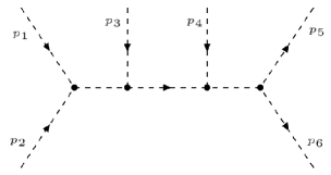
Figure 1: $6$-point amplitude for scalar cubic interaction. The blobs correspond to dressed vertices.

We now wish to compute $N$-point amplitudes, $\mathcal{M}_{N},$ for the action in Eq.(2). Let us consider $n=1$ to start with, and then we will generalize to generic powers of $\Box$. A generic tree-level $N$-point amplitude for the action in Eq.(2) will be made of $N$ external legs, $N-2$ vertices and $N-3$ internal propagators; see Fig. $1$. The simplest scattering amplitude we can construct is a $4$-point diagram, whose behavior in the UV regime is given by:

$$\mathcal{M}_{4}\leavevmode\nobreak\ \leavevmode\nobreak\ \xrightarrow{UV}\leavevmode\nobreak\ \leavevmode\nobreak\ \lambda^{6}\frac{e^{-\frac{5}{3}p^{2}/M_{s}^{2}}}{p^{2}},$$ (11)

with $p$ being the sum of the two ingoing (or, equivalently, outgoing) momenta, $p_{1}+p_{2}=p_{3}+p_{4}\equiv p.$ Similarly, by increasing the number of external legs to $6$, we can consider a $6$-point amplitude as in Fig. $1$ , where our convention is that all $p_{i}$ with $i=1,2,3,4$ are ingoing, while $p_{5}$ and $p_{6}$ are outgoing momenta. From the conservation law of the total $4$-momentum, we have:

$$p_{1}+p_{2}+p_{3}+p_{4}=p_{5}+p_{6}.$$ (12)

The $6$-point amplitude in the UV regime then reads:

$$\!\!\mathcal{M}_{6}\!\xrightarrow{UV}\!\lambda^{12}\!\frac{e^{-\frac{5}{3}\frac{(p_{1}+p_{2})^{2}}{M_{s}^{2}}}e^{-\frac{5}{3}\frac{(p_{1}+p_{2}+p_{3})^{2}}{M_{s}^{2}}}e^{-\frac{5}{3}\frac{(p_{1}+p_{2}+p_{3}+p_{4})^{2}}{M_{s}^{2}}}}{(p_{1}+p_{2})^{2}(p_{1}+p_{2}+p_{3})^{2}(p_{1}+p_{2}+p_{3}+p_{4})^{2}}.$$ (13)

For simplicity, we can make the following choice for the incoming momenta:

$$|p_{1}+p_{2}|=|p_{3}+p_{4}|\equiv|p|,\,\,\,\,\vec{p}_{1}=-\vec{p}_{2},\,\,\,\,\vec{p}_{3}=-\vec{p}_{4};$$ (14)

thus, the amplitude in Eq.(13) is roughly given by

$$\mathcal{M}_{6}\sim\frac{\lambda^{12}}{(2!)^{2}}\frac{e^{-\frac{5}{3}(2(1)^{2}+2^{2})p^{2}/M_{s}^{2}}}{p^{6}}=\frac{\lambda^{12}}{(2!)^{2}}\frac{e^{-10p^{2}/M_{s}^{2}}}{p^{6}},$$ (15)

where we have neglected the terms such as $(p_{3}^{4})^{2}$ and $2p_{3}^{4}p$ as $2p^{2}>(p_{3}^{4})^{2},\,2p_{3}^{4}p$, and this approximation becomes even more justified for a very large number of external legs, i.e. when $N\gg 1$; see below. By adding two extra external legs, $p_{7}$ and $p_{8}$, and making similar choices as in Eq.(14) and neglecting the cross-terms, one can see that the $8$-point scattering amplitude will behave as

$$\mathcal{M}_{8}\sim\frac{\lambda^{18}}{(3!)^{2}}\frac{e^{-\frac{5}{3}(2(1^{2}+2^{2})+3^{2})p^{2}/M_{s}^{2}}}{p^{10}}=\frac{\lambda^{18}}{(3!)^{2}}\frac{e^{-\frac{95}{3}p^{2}/M_{s}^{2}}}{p^{10}}.$$ (16)

By inspecting Eqs. (15, 16), it is clear that by increasing the number of external legs, the scattering amplitude becomes even more exponentially suppressed. We can now easily find the expression for an $N$-point scattering amplitude, which will be roughly given by

$$\begin{array}[]{rl}\mathcal{M}_{N}=&\displaystyle V_{\rm dress}(p_{1},p_{2},p_{1}+p_{2})\prod\limits_{i=2}^{N-2}\Pi_{\rm dress}(p_{1}+\cdots+p_{i})\\ &\displaystyle\times\prod_{j=2}^{N-3}V_{\rm dress}(p_{1}+\cdots+p_{j},\,p_{j+1},\,p_{1}+\cdots+p_{j+1})\\ &\displaystyle\times V_{\rm dress}(p_{1}+\cdots+p_{N-2},p_{N-1},p_{N})\\ \xrightarrow{UV}&\displaystyle\frac{\lambda^{3(N-2)}}{[(N-2)/2]!^{2}}\frac{e^{-\frac{10}{3}\left(\sum\limits_{l=1}^{\frac{N-2}{2}}l^{2}-\frac{1}{2}\left(\frac{N-2}{2}\right)^{2}\right)p^{2}/M_{s}^{2}}}{p^{2(N-3)}},\end{array}$$ (17)

where now the conservation law of the $4$-momenta in Eq.(12) and the choice in Eq.(14) generalize to

$$p_{1}+p_{2}+\cdots+p_{N-2}=p_{N-1}+p_{N}$$ (18)

and

$$|p_{i}+p_{i+1}|\equiv|p|,\,\,\,\,\vec{p}_{i}=-\vec{p}_{i+1},\,\,\,\,i=1,\dots,N-3;$$ (19)

and we have used the relation

$$2j^{2}p^{2}\gg(p_{2j+1}^{4})^{2},\,2p^{4}_{2j+1}jp,$$ (20)

to neglect terms like $(p_{2j+1}^{4})^{2}$ and $2p^{4}_{2j+1}jp,$ as $j\gg 1.$ Note that the second set of equalities in Eq.(19) corresponds to the choice of the centre of mass frame for $N-2$ incoming particles; indeed, for two incoming particles we would only have $\vec{p}_{1}=-\vec{p}_{2}$ and recover the usual relation between the spatial part of the two incoming momenta in the case of a $4$-point scattering amplitude.

The numeric series in Eq.(17) can be summed up and in the limit $N\gg 1$ reads:

$$\sum\limits_{l=1}^{\frac{N-2}{2}}l^{2}=\frac{N(N-1)(N-2)}{12}\,\xrightarrow{N\gg 1}\,N^{3};$$ (21)

therefore, for a large number of interacting particles the $N$-point amplitude in Eq.(17) shows the following behavior:

$$\mathcal{M}_{N}\sim\lambda^{\prime}\frac{e^{-N^{3}p^{2}/M_{s}^{2}}}{p^{2(N-3)}}=\lambda^{\prime}\frac{e^{-p^{2}/M_{\rm eff}^{2}}}{p^{2(N-3)}},$$ (22)

where we have defined $\lambda^{\prime}:=\lambda^{3(N-2)}/[(N-2)/2]!^{2}$ and in the last step we have introduced the effective scale

$$M_{\rm eff}\sim\frac{M_{s}}{N^{{3}/{2}}}.$$ (23)

Hence, from Eqs.(22, 23) we have obtained that by increasing the number of external legs, or in other words the number of interacting particles, the scattering amplitude becomes more exponentially suppressed. This feature can be understood as follows: there is a transmutation of scale under which the fundamental scale of nonlocality $M_{s}$ shifts towards lower energies, i.e. $M_{\rm eff}\ll M_{s}$ when $N\gg 1$. In this process, the nonlocal length and time scales can be made much larger than the original scale of nonlocality, i.e. $M_{s}^{-1}\longrightarrow N^{3/2}M_{s}^{-1}$, therefore its affect can be felt in the IR. This phenomena of transmuting the scale from UV to IR has been shown in the fuzz ball construction in string theory setup to resolve blackhole singularity and horizon Mathur:2005zp .

The above calculations are performed for the form-factor $e^{-\Box/M_{s}^{2}},$ i.e. with $n=1.$ We can generalize straightforwardly the previous results to generic powers $n$ of the d’Alembertian, such as $e^{(-\Box/M_{s}^{2})^{n}}:$

$$\mathcal{M}_{N}\sim\lambda^{\prime}\frac{e^{-\frac{10}{3}\left(\sum\limits_{l=1}^{\frac{N-2}{2}}l^{2n}\right)p^{2n}/M_{s}^{2n}}}{p^{2(N-3)}}.$$ (24)

The numeric series in Eq.(24) can be expressed in terms of the Faulhaber formula which is given by numbers

$$\!\sum\limits_{l=1}^{\frac{N-2}{2}}l^{2n}=\frac{1}{2n+1}\sum\limits_{i=0}^{2n}(-1)^{i}{2n+1\choose i}B_{i}\cdot\left(\frac{N}{2}-1\right)^{2n+1-i}\!,$$ (25)

where $B_{i}$ is the so called Bernoulli number. The expression in Eq.(25) seems rather complicated, but fortunately we are only interested in the limit $N\gg 1,$ which gives

$$\sum\limits_{l=1}^{\frac{N-2}{2}}l^{2n}\,\xrightarrow{N\gg 1}\,N^{2n+1}.$$ (26)

Hence, the $N$-point scattering amplitude for generic powers $n$ of the d’Alembertian will behave as

$$\mathcal{M}_{N}\sim\lambda^{\prime}\frac{e^{-(N^{2n+1})p^{2n}/M_{s}^{2n}}}{p^{2(N-3)}}=\lambda^{\prime}\frac{e^{-p^{2n}/M_{\rm eff}^{2n}}}{p^{2(N-3)}},$$ (27)

where in this more general case the effective nonlocal scale is defined as:

$$M_{\rm eff}\sim\frac{M_{s}}{N^{\frac{2n+1}{2n}}}=\frac{M_{s}}{N^{1+{1}/{2n}}}.$$ (28)

III.2 Zero external momenta

We now wish to ask a similar question but for a different kind of amplitude, with zero ingoing and outgoing external momenta. As done before, let us start when $n=1$, and consider a tree-level diagram as the one in Fig. $1$, but with a different choice of the external momenta. For this kind of diagram (with no loops) we can not set all single momentum equal to zero, otherwise we would not get any exponential contributions, but we will consider the following choice:

$$p_{1}+\cdots+p_{N-2}=p_{N-1}+p_{N},$$ (29)

$$|p_{i}+p_{i+1}|\equiv|p|,\,\,\,\,\,i=1,\dots,N-3,$$ (30)

and

$$\begin{array}[]{ll}\displaystyle p_{N}=-p_{N-1},&\\ \displaystyle p_{i}+p_{i+1}=-(p_{i+2}+p_{i+3}),\,\,\,\,i=1,\dots,N-5;&\end{array}$$ (31)

with on-shell conditions $p_{i}^{2}=0.$

For the above choice of momentum distribution in Eq.(31), the IR divergences from the denominators may appear. However, they can be cured as in the standard local field theory where non locality does not play any role. Indeed they are just related to the fact that we are working with a massless scalar field. Anyway, we are interested in the regime where nonlocality in the propagator becomes important, and want to understand the role played by the exponential form-factors.

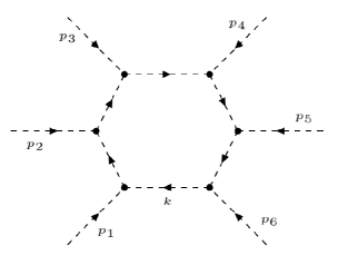
Figure 2: Ring diagram: $1$-loop $6$-point amplitude for scalar cubic interaction. The blobs correspond to dressed vertices.

In fact, in this regime the tree-level $N$-point amplitude, in the limit $N\gg 1,$ will be given by

$$\mathcal{M}_{N}\xrightarrow{N\gg 1}\lambda^{3(N-2)}e^{-Np^{2}/M_{s}^{2}}=\lambda^{3(N-2)}e^{-p^{2}/M_{\rm eff}^{2}},$$ (32)

where we have introduced the effective scale

$$M_{\rm eff}\sim\frac{M_{s}}{\sqrt{N}}.$$ (33)

Hence, in the case of zero ingoing and outgoing external momenta the total amplitude becomes more suppressed for an increasing number of interacting particles, but by comparing to the previous case, see Eq.(23), the scaling is different.

Furthermore, we can show that similar transmutation of the scale manifest also for different amplitudes, as for the $1$-loop diagram of the kind in Fig.$2$, known as the ring diagram. In this case, given $N$ external legs we have $N$ vertices and $N$ internal propagators. Since we have a loop in the diagram, we can now set all individual external momenta to zero, and we can show that an $N$-point amplitude as the one in Fig. $2$, with $p_{i}=0,$ $i=1,\dots,N,$ reads:

$$\begin{array}[]{rl}\mathcal{M}_{{\rm ring},\,N}\sim&\displaystyle\lambda^{3N}\int\frac{d^{4}k}{(2\pi)^{4}}\frac{e^{-Nk^{2}/M_{s}^{2}}}{k^{2N}}\\ =&\displaystyle\lambda^{3N}\int\frac{d^{4}k}{(2\pi)^{4}}\frac{e^{-k^{2}/M_{\rm eff}^{2}}}{k^{2N}},\end{array}$$ (34)

where the effective scale $M_{\rm eff}$ coincides with the one in Eq.(33).

Figure 3: The dashed blob represents the region in which the nonlocal interaction takes place. The larger is the number of interacting particles, the larger will be the nonlocal region in coordinate space and time.

So far we have only considered the scaling properties for $n=1,$ but we can straightforwardly generalize the above results to generic $\Box^{n}$. We can show that for an $N$-point amplitude with zero external momenta, the scale of nonlocality will transmute to

$$M_{\rm eff}\sim\frac{M_{s}}{N^{1/2n}}.$$ (35)

IV Scalar toy-model for infinite derivative gravity

We now wish to consider a slightly more interesting scenario of a scalar toy-model, which can mimic the graviton self-interaction in ghost-free infinite derivative gravity (IDG), up to cubic order $\mathcal{O}(h^{3}),$ where $h$ is the trace $h=\eta^{\mu\nu}h_{\mu\nu}$ of the graviton perturbation around the Minkowski background, which is now mimed by the scalar field $\phi(x).$ Such a model was first studied in Refs. Talaganis:2014ida ; Talaganis:2016ovm and the corresponding Euclidean action reads Talaganis:2014ida  

$$\begin{array}[]{rl}S=&\displaystyle\int d^{4}x\left(\frac{1}{2}\phi(x)e^{\left(-\Box/M_{s}^{2}\right)^{n}}\Box\phi(x)\right.\\ &+\displaystyle\frac{\lambda}{4}\phi(x)\partial_{\mu}\phi(x)\partial^{\mu}\phi(x)\\ &\displaystyle+\frac{\lambda}{4}\phi(x)\Box\phi(x)e^{\left(-\Box/M_{s}^{2}\right)^{n}}\phi(x)\\ &\displaystyle\left.-\frac{\lambda}{4}\phi(x)\partial_{\mu}\phi(x)e^{\left(-\Box/M_{s}^{2}\right)^{n}}\partial^{\mu}\phi(x)\right).\end{array}$$ (36)

The above action exhibits the following scaling symmetry: $\phi\longrightarrow(1+\epsilon)\phi+\epsilon$ Talaganis:2014ida . The Euclidean bare propagator for this action is the same as the one in Eq.(3), while the bare vertex is not a constant, but it is given by Talaganis:2014ida ; Talaganis:2016ovm

$$\!\!\begin{array}[]{rl}V(k_{1},k_{2},k_{3})=&\displaystyle\frac{\lambda}{4}\left(k_{1}^{2}+k_{2}^{2}+k_{3}^{2}\right)\left(e^{k^{2n}_{1}/M_{s}^{2n}}+e^{k^{2n}_{2}/M_{s}^{2n}}\right.\\ &\displaystyle\,\,\,\,\,\,\,\,\,\,\,\,\,\,\,\,\,\,\,\,\,\,\,\,\,\,\,\,\,\,\,\,\,\,\,\,\,\,\,\,\,\,\,\,\,\,\,\left.+e^{k^{2n}_{3}/M_{s}^{2n}}-1\right).\end{array}$$ (37)

Even though the propagator is exponentially suppressed, the vertex function is exponentially enhanced. We will make explicit computations for the power $n=1$, and then generalize to any power of $\Box^{n}$.

IV.0.1 Dressing the propagators

Unlike the case of the cubic interaction in Section III (see Eq.(2)), in the case of the above action in Eq.(36), the UV behavior of the propagator is slightly modified by loop quantum corrections, as shown in Refs. Talaganis:2014ida ; Talaganis:2016ovm . First of all, the self-energy at $1$-loop for the action in Eq.(36) is given by

$$\Sigma^{(1)}(p)=\displaystyle\int\frac{d^{4}k}{(2\pi)^{4}}\frac{V^{2}(p,k,k-p)}{k^{2}(k-p)^{2}}e^{-\frac{k^{2}}{M_{s}^{2}}}e^{-\frac{(k-p)^{2}}{M_{s}^{2}}}.$$ (38)

The above integral can be exactly computed and reads Talaganis:2014ida

$$\!\!\!\begin{array}[]{ll}\displaystyle\Sigma^{(1)}(p)=\displaystyle\frac{\lambda^{2}}{16\pi^{2}}\left\{\frac{p^{4}}{8}\left({\rm log}\left(\frac{p^{2}}{4\pi M_{s}^{2}}\right)+\gamma_{E}-2\right)\right.&\\[8.53581pt] \,\,\displaystyle+\frac{e^{-p^{2}/M_{s}^{2}}M^{2}_{s}}{32p^{2}}\left[2M_{s}^{2}p^{2}e^{p^{2}/M_{s}^{2}}\left(e^{2p^{2}/M_{s}^{2}}-1\right){\rm Ei}\left(-\frac{p^{2}}{M_{s}^{2}}\right)\right.&\\[8.53581pt] \,\displaystyle-\left(e^{p^{2}/M_{s}^{2}}-1\right)\left(M_{s}^{2}p^{2}e^{p^{2}/M_{s}^{2}}\left(e^{p^{2}/M_{s}^{2}}-1\right){\rm Ei}\left(-\frac{p^{2}}{2M_{s}^{2}}\right)\right.&\\[8.53581pt] \,\,\displaystyle+\left(e^{\frac{3}{2}p^{2}/M_{s}^{2}}-e^{p^{2}/2M_{s}^{2}}\right)\left(2p^{4}+5M_{s}^{2}p^{2}+4M_{s}^{4}\right)&\\[8.53581pt] \,\,\,\,\,\,\,\,\,\,\,\,\displaystyle+2e^{p^{2}/M_{s}^{2}}\left(7p^{4}+7M_{s}^{2}p^{2}+2M_{s}^{2}\right)&\\[8.53581pt] \,\,\,\,\,\,\,\,\,\,\displaystyle\left.\left.\left.-2\left(p^{4}+3M_{s}^{2}p^{2}+2M_{s}^{4}\right)\right)\right]\right\},&\end{array}$$ (39)

where $\gamma_{E}=0.57721\dots$ is the Euler-Mascheroni constant. Although the above expression is very complicated, in the UV regime the behavior of the $1$-loop self-energy turns out to be simpler and is given by

$$\Sigma^{(1)}(p)\xrightarrow{UV}\displaystyle\lambda^{2}e^{\frac{3}{2}p^{2}/M_{s}^{2}},$$ (40)

where we have neglected numerical factors. With the help of Eqs.(LABEL:1-loop_self-energy-deriv),(40), we can now compute the dressed propagator, whose UV behavior is given by

$$\Pi_{\rm dress}(p)\leavevmode\nobreak\ \leavevmode\nobreak\ \xrightarrow{UV}\leavevmode\nobreak\ \leavevmode\nobreak\ \lambda^{-2}e^{-\frac{3}{2}p^{2}/M_{s}^{2}},$$ (41)

which turns out to be even more exponentially suppressed than the bare one, as we now have the factor $3/2$ in the exponent as compared to Eq.(3).

IV.0.2 Dressing the vertices

In Ref. Talaganis:2016ovm , it was shown that eventhough a bare vertex is exponentially enhanced the dressed vertex can be exponentially suppressed, provided higher order quantum loops, built with dressed propagators, are taken into account. In fact, in the UV regime the dressed vertex has the following form Talaganis:2016ovm :

$$V_{\rm dress}^{(l)}(k_{1},k_{2},k_{3})\leavevmode\nobreak\ \leavevmode\nobreak\ \xrightarrow{UV}\leavevmode\nobreak\ \leavevmode\nobreak\ \lambda^{3}e^{\alpha^{(l)}\frac{k_{1}^{2}}{M_{s}^{2}}+\beta^{(l)}\frac{k_{2}^{2}}{M_{s}^{2}}+\gamma^{(l)}\frac{k_{3}^{2}}{M_{s}^{2}}},$$ (42)

where $l$ is the number of loops, or in other words, the loop order. If $l\geq 4$, the dressed vertex becomes exponentially suppressed; for instance, if $l=4$ we obtain Talaganis:2014ida ; Talaganis:2016ovm :

$$\alpha^{(4)}=\beta^{(4)}=\gamma^{(4)}=-\frac{11}{27},$$ (43)

so that the dressed vertex takes the following form in the UV:

$$V_{\rm dress}^{(4)}(k_{1},k_{2},k_{3})\leavevmode\nobreak\ \leavevmode\nobreak\ \xrightarrow{UV}\leavevmode\nobreak\ \leavevmode\nobreak\ \lambda^{3}e^{-\frac{11}{27}\left(\frac{k_{1}^{2}}{M_{s}^{2}}+\frac{k_{2}^{2}}{M_{s}^{2}}+\frac{k_{3}^{2}}{M_{s}^{2}}\right)}.$$ (44)

IV.1 $N$-point scattering amplitude

By assuming first the simple case, $n=1,$ we will compute the $4$-point scattering amplitude, with momenta $p_{1}+p_{2}=p_{3}+p_{4}\equiv p,$ where we use both dressed propagators and vertices, the latter at the loop order $l=4$:

$$\begin{array}[]{rl}\mathcal{M}_{4}=&\displaystyle V_{\rm dress}^{(4)}(p_{1},p_{2},p)\Pi_{\rm dress}(p)V_{\rm dress}^{(4)}(p,p_{3},p_{4})\\[8.53581pt] \,\,\xrightarrow{UV}&\displaystyle\lambda^{4}e^{-\left((2)\frac{11}{27}+\frac{3}{2}\right)p^{2}/M_{s}^{2}}\sim\lambda^{4}e^{-\frac{125}{54}p^{2}/M_{s}^{2}},\end{array}$$ (45)

which turns out to be exponentially suppressed in Euclidean signature, where we have used the on-shell condition $p_{i}^{2}=0.$ Let us now consider the dressed $N$-point amplitude, with $N>4:$

$$\!\!\!\begin{array}[]{ll}\mathcal{M}_{N}=\displaystyle V_{\rm dress}^{(4)}(p_{1},p_{2},p_{1}+p_{2})\prod\limits_{i=2}^{N-2}\Pi_{\rm dress}(p_{1}+\cdots+p_{i})&\\ \,\,\,\,\,\,\times\displaystyle\prod_{j=2}^{N-3}V_{\rm dress}^{(4)}(p_{1}+\cdots+p_{j},\,p_{j+1},\,p_{1}+\cdots+p_{j}+p_{j+1})&\\ \,\,\,\,\,\,\times\displaystyle V_{\rm dress}^{(4)}(p_{1}+\cdots+p_{N-2},p_{N-1},p_{N});&\end{array}$$ (46)

when $N=4$ the product in the second line is just one, and we recover the result in Eq.(45). By imposing the on-shell conditions $p_{i}^{2}=0$, and making the choices for momenta as in Eqs. (19, 20), the UV behavior of the $N$-point amplitude in Eq.(46) reads:

$$\mathcal{M}_{N}\leavevmode\nobreak\ \leavevmode\nobreak\ \xrightarrow{UV}\leavevmode\nobreak\ \leavevmode\nobreak\ \lambda^{N}e^{-\frac{125}{27}\left(\sum\limits_{l=1}^{\frac{N-2}{2}}l^{2}-\frac{1}{2}\left(\frac{N-2}{2}\right)^{2}\right)p^{2}/M_{s}^{2}}.$$ (47)

By assuming the limit $N\gg 1$, we obtain

$$\mathcal{M}_{N}\leavevmode\nobreak\ \leavevmode\nobreak\ \xrightarrow{N\gg 1}\leavevmode\nobreak\ \leavevmode\nobreak\ \lambda^{N}e^{-N^{3}p^{2}/M_{s}^{2}}=\lambda^{N}e^{-p^{2}/M_{\rm eff}^{2}}.$$ (48)

where we have introduced the effective scale

$$M_{\rm eff}\sim\frac{M_{s}}{N^{{3}/{2}}},$$ (49)

which coincides with the scaling in Eq.(23).

So far we have only considered $n=1$ case, the calculations are complicated for generic powers of $n$ of the d’Alembertian. However, we can still understand the problem by observing that the UV behaviors of dressed propagators and vertices are proportional to $e^{-c\left(p^{2}/M_{s}^{2}\right)^{n}},$ with some positive numerical factor, $c>0.$ Thus, we can generalize our results to generic powers of $n,$ and show that the scaling still coincides with the one obtained for the action in Eq.(2) (see Eq.(28)):

$$M_{\rm eff}\sim\frac{M_{s}}{N^{\frac{2n+1}{2n}}}.$$ (50)

IV.2 Zero external momenta

We now wish to compute the $N$-point amplitudes with zero ingoing and outgoing external momenta. In the UV when $N\gg 1$, the amplitude follows the same behavior as the one for the scalar action in Section III. Indeed, by dressing both internal propagators and vertices as done in Eqs.(41, 44), we can show that we get a similar result as in Eqs.(32, 34). For instance, the ring diagram in Fig. $2$ with zero external momenta reads:

$$\begin{array}[]{rl}\mathcal{M}_{{\rm ring},\,N}\sim&\displaystyle\lambda^{N}\int\frac{d^{4}k}{(2\pi)^{4}}e^{-\frac{125}{54}Nk^{2n}/M_{s}^{2n}}\\ \xrightarrow{N\gg 1}&\displaystyle\lambda^{N}\int\frac{d^{4}k}{(2\pi)^{4}}e^{-k^{2n}/M_{\rm eff}^{2n}}.\end{array}$$ (51)

Thus, the scale of nonlocality now transmutes as in our previous case, see Eq.(35)):

$$M_{\rm eff}\sim\frac{M_{s}}{N^{\frac{1}{2n}}}.$$ (52)

V Discussions and Conclusions

In this paper we have computed the $N$-point amplitudes in the context of ghost-free infinite derivative scalar field theories. We have worked with a massless scalar field and studied two toy models in Eqs.(2, 36). In particular, we were interested in the limit in which the number of particles, $N,$ could be very large and we have shown that the scale of nonlocality, $M_{s},$ transmutes to a lower value in the IR depending on $N$, and on the form of the entire function. Although, $M_{s}$ represents a physical cut-off and beyond which it is hard to probe the nature of physics, but with a large number of interacting particles/quanta the nonlocal regime becomes more accessible in the IR.

The above computations also provide a tangible support to IDG theories, where the scale of nonlocality may be a dynamical quantity and can be modified in presence of a large number of gravitons interacting nonlocally, as argued from completely different point of view - by arguing that the entropy of a gravitationally bound system would follow the Area-law Koshelev:2017bxd . This result has already played a key role in constructing non-singular compact objects Koshelev:2017bxd ; Buoninfante:2018rlq . However, explicit scattering amplitude computations for $N$-point amplitudes in the context of nonlocal gravitational interaction are still lacking and will be the subject of future works.

- (1) H. Yukawa, Phys. Rev. 77, 219 (1950). H. Yukawa, Phys. Rev. 80, 1047 (1950).
- (2) R.P. Feynman and J.A. Wheeler, Rev. Mod. Phys. 17 (1945) 157; A. Pais and G. E. Uhlenbeck, Phys. Rev. 79, 145 (1950); V. Efimov, Comm. Math. Phys. 5, 42 (1967); V. Efimov, ibid, 7, 138 (1968); V. A. Alebastrov, V. Efimov, Comm. Math. Phys. 31, 1, 1-24 (1973); V. A. Alebastrov, V. Efimov, Comm. Math. Phys. 38, 1, 11-28 (1974); D. A. Kirzhnits (1967) Sov. Phys. Usp. 9 692.
- (3) N. V. Krasnikov, Theor Math. Phys. 73 1184, 1987, Teor. Mat. Fiz. 73, 235 (1987).
- (4) Yu. V. Kuzmin, Yad. Fiz. 50, 1630-1635 (1989).
- (5) J. W. Moffat, ”Finite nonlocal gauge field theory,” Phys. Rev. D 41, 1177 (1990). D. Evens, J. W. Moffat, G. Kleppe and R. P. Woodard, ”Nonlocal regularizations of gauge theories,” Phys. Rev. D 43, 499 (1991).
- (6) E. T. Tomboulis, ”Superrenormalizable gauge and gravitational theories,” hep-th/9702146.
- (7) T. Biswas and N. Okada, ”Towards LHC physics with nonlocal Standard Model,” Nucl. Phys. B 898, 113 (2015), [arXiv:1407.3331 [hep-ph]].
- (8) E. T. Tomboulis, Phys. Rev. D 92, no. 12, 125037 (2015) [arXiv:1507.00981 [hep-th]].
- (9) A. Ghoshal, A. Mazumdar, N. Okada and D. Villalba, Phys. Rev. D 97, no. 7, 076011 (2018) [arXiv:1709.09222 [hep-th]].
- (10) L. Buoninfante, G. Lambiase and A. Mazumdar, ”Ghost-free infinite derivative quantum field theory”, arXiv:1805.03559 [hep-th].
- (11) E. Witten, Nucl. Phys. B 268, 253 (1986).
- (12) P. G. O. Freund and M. Olson, Phys. Lett. B 199, 186 (1987). L. Brekke, P. G. O. Freund, M. Olson and E. Witten, Nucl. Phys. B 302, 365 (1988). P. G. O. Freund and E. Witten, Phys. Lett. B 199, 191 (1987). P. H. Frampton and Y. Okada, Effective Scalar Field Theory of P ? adic String, Phys.Rev., vol. D37, pp. 3077? 3079, 1988.
- (13) D.A. Eliezer, R.P. Woodard, Nucl. Phys. B, 325 389 (1989).
- (14) A. A. Tseytlin, “On singularities of spherically symmetric backgrounds in string theory,” Phys. Lett. B 363 (1995) 223, [hep-th/9509050].
- (15) W. Siegel, “Stringy gravity at short distances,” hep-th/0309093.
- (16) T. Biswas, A. Mazumdar and W. Siegel, JCAP 0603, 009 (2006) [hep-th/0508194].
- (17) T. Biswas, E. Gerwick, T. Koivisto and A. Mazumdar, “Towards singularity and ghost free theories of gravity,” Phys. Rev. Lett. 108, 031101 (2012).
- (18) L. Modesto, ”Super-renormalizable Quantum Gravity”, Phys. Rev. D 86, 044005 (2012).
- (19) T. Biswas, A. S. Koshelev and A. Mazumdar, Fundam. Theor. Phys. 183, 97 (2016). T. Biswas, A. S. Koshelev and A. Mazumdar, Phys. Rev. D 95, no. 4, 043533 (2017).
- (20) R. Pius and A. Sen, a Cutkosky Rules for Superstring Field Theory,” High Energ. Phys. (2016) [arXiv:1604.01783[hep-th]]. A. Sen, ”One Loop Mass Renormalization of Unstable Particles in Superstring Theory”, J. High Energ. Phys. (2016), [arXiv:1607.06500 [hep-th]].
- (21) C. D. Carone, ”Unitarity and microscopic acausality in a nonlocal theory”, Phys. Rev. D 95, 045009 (2017), [arXiv:1605.02030v3 [hep-th]].
- (22) P. Chin and E. T. Tomboulis, ”Nonlocal vertices and analyticity: Landau equations and general Cutkosky rule,” JHEP 1806 (2018) 014, [arXiv:1803.08899 [hep-th]].
- (23) F. Briscese and L. Modesto, ”Cutkosky rules and perturbative unitarity in Euclidean nonlocal quantum field theories,” arXiv:1803.08827 [gr-qc].
- (24) T. Biswas, T. Koivisto and A. Mazumdar, “Nonlocal theories of gravity: the flat space propagator,” arXiv:1302.0532 [gr-qc].
- (25) S. Talaganis, T. Biswas and A. Mazumdar, ”Towards understanding the ultraviolet behavior of quantum loops in infinite-derivative theories of gravity,” Class. Quant. Grav. 32, no. 21, 215017 (2015) [arXiv:1412.3467 [hep-th]].
- (26) T. Biswas, A. Conroy, A. S. Koshelev and A. Mazumdar, Class. Quant. Grav. 31, 015022 (2014), Erratum: [Class. Quant. Grav. 31, 159501 (2014)]. [arXiv:1308.2319 [hep-th]].
- (27) J. Edholm, A. S. Koshelev and A. Mazumdar, Phys. Rev. D 94, no. 10, 104033 (2016). V. P. Frolov and A. Zelnikov, Phys. Rev. D 93, no. 6, 064048 (2016).
- (28) A. Mazumdar and G. Stettinger, “New massless and massive infinite derivative gravity in three dimensions around Minkowski and in (A)dS,” arXiv:1811.00885 [hep-th].
- (29) V. P. Frolov, A. Zelnikov and T. de Paula Netto, JHEP 1506, 107 (2015) [arXiv:1504.00412 [hep-th]].
- (30) V. P. Frolov, Phys. Rev. Lett. 115, no. 5, 051102 (2015).
- (31) V. P. Frolov and A. Zelnikov, Phys. Rev. D 93, no. 6, 064048 (2016) [arXiv:1509.03336 [hep-th]].
- (32) L. Buoninfante, Master’s Thesis (2016), [arXiv:1610.08744v4 [gr-qc]].
- (33) A. S. Koshelev and A. Mazumdar, Do massive compact objects without event horizon exist in infinite derivative gravity?, Phys. Rev. D 96, no. 8, 084069 (2017), [arXiv:1707.00273 [gr-qc]].
- (34) L. Buoninfante, A. S. Koshelev, G. Lambiase and A. Mazumdar, “Classical properties of non-local, ghost- and singularity-free gravity,” JCAP 1809 (2018) no.09, 034, [arXiv:1802.00399 [gr-qc]].
- (35) A. S. Koshelev, J. Marto and A. Mazumdar, “Schwarzschild -singularity is not permissible in ghost free quadratic curvature infinite derivative gravity,” Phys. Rev. D 98 (2018) no.6, 064023 doi:10.1103/PhysRevD.98.064023 [arXiv:1803.00309 [gr-qc]].
- (36) L. Buoninfante, A. S. Koshelev, G. Lambiase, J. Marto and A. Mazumdar, “Conformally-flat, non-singular static metric in infinite derivative gravity,” JCAP 1806 (2018) no.06, 014 doi:10.1088/1475-7516/2018/06/014 [arXiv:1804.08195 [gr-qc]].
- (37) L. Buoninfante, G. Harmsen, S. Maheshwari and A. Mazumdar, Phys. Rev. D 98 (2018) no.8, 084009 [arXiv:1804.09624 [gr-qc]].
- (38) B. L. Giacchini and T. de Paula Netto, arXiv:1809.05907 [gr-qc].
- (39) A. S. Cornell, G. Harmsen, G. Lambiase and A. Mazumdar, Phys. Rev. D 97, no. 10, 104006 (2018) doi:10.1103/PhysRevD.97.104006 [arXiv:1710.02162 [gr-qc]]. L. Buoninfante, A. S. Cornell, G. Harmsen, A. S. Koshelev, G. Lambiase, J. Marto and A. Mazumdar, Phys. Rev. D 98, no. 8, 084041 (2018), arXiv:1807.08896 [gr-qc].
- (40) J. Boos, V. P. Frolov and A. Zelnikov, ”The gravitational field of static p-branes in linearized ghost-free gravity,” Phys. Rev. D 97, no. 8, 084021 (2018) doi:10.1103/PhysRevD.97.084021 [arXiv:1802.09573 [gr-qc]].
- (41) T. Biswas, T. Koivisto and A. Mazumdar, “Towards a resolution of the cosmological singularity in non local higher derivative theories of gravity,” JCAP 1011, 008 (2010), [arXiv:1005.0590 [hep-th]].
- (42) T. Biswas, A. S. Koshelev, A. Mazumdar and S. Y. Vernov, “Stable bounce and inflation in non local higher derivative cosmology,” JCAP 1208, 024 (2012), [arXiv:1206.6374 [astro-ph.CO]].
- (43) A. S. Koshelev and S. Y. Vernov, “On bouncing solutions in non local gravity,” Phys. Part. Nucl. 43, 666 (2012), [arXiv:1202.1289 [hep-th]].
- (44) A. S. Koshelev, J. Marto and A. Mazumdar, ”Towards resolution of anisotropic cosmological singularity in infinite derivative gravity,” arXiv:1803.07072 [gr-qc].
- (45) S. Talaganis and A. Mazumdar, ”High-Energy Scatterings in Infinite-Derivative Field Theory and Ghost-Free Gravity,” Class. Quant. Grav. 33, no. 14, 145005 (2016), [arXiv:1603.03440 [hep-th]].
- (46) T. Biswas, J. A. R. Cembranos and J. I. Kapusta, Phys. Rev. Lett. 104, 021601 (2010) doi:10.1103/PhysRevLett.104.021601 [arXiv:0910.2274 [hep-th]].
- (47) T. Biswas, J. A. R. Cembranos and J. I. Kapusta, JHEP 1010, 048 (2010) doi:10.1007/JHEP10(2010)048 [arXiv:1005.0430 [hep-th]].
- (48) T. Biswas, J. A. R. Cembranos and J. I. Kapusta, Phys. Rev. D 82, 085028 (2010) doi:10.1103/PhysRevD.82.085028 [arXiv:1006.4098 [hep-th]].
- (49) N. Barnaby, T. Biswas and J. M. Cline, ”p-adic Inflation,” JHEP 0704 (2007) 056 [hep-th/0612230]; J. E. Lidsey, ”Stretching the inflaton potential with kinetic energy,” Phys. Rev. D 76 (2007) 043511 [hep-th/0703007]; L. Joukovskaya, ”Dynamics in nonlocal cosmological models derived from string field theory,” Phys. Rev. D 76 (2007) 105007 [arXiv:0707.1545 [hep-th]]; G. Calcagni, M. Montobbio and G. Nardelli, ”A Route to nonlocal cosmology,” Phys. Rev. D 76 (2007) 126001 [arXiv:0705.3043 [hep-th]]; T. Biswas, R. Brandenberger, A. Mazumdar and W. Siegel, “Non-perturbative Gravity, Hagedorn Bounce & CMB,” JCAP 0712, 011 (2007) [hep-th/0610274].
- (50) S. D. Mathur, Fortsch. Phys. 53, 793 (2005), [hep-th/0502050].
- (51) J. H. Conway, R. Guy, ”The Book of Numbers,” Springer (1996), p. 107. ISBN 0-387-97993-X.
- (52) S. Talaganis and A. Teimouri, “Scale of non-locality for a system of particles,” arXiv:1705.07759 [hep-th].