$AdS_{4}$ dyonic black holes in gravity’s rainbow

Abstract

In this paper, we investigate thermodynamical structure of dyonic black holes in the presence of gravity’s rainbow. We confirm that for super magnetized and highly pressurized scenarios, the number of black holes’ phases is reduced to a single phase. In addition, due to specific coupling of rainbow functions, it is possible to track the effects of temporal and spatial parts of our setup on thermodynamical quantities/behaviors including equilibrium point, existence of multiple phases, possible phase transitions and conditions for having a uniform stable structure.

I Introduction

General relativity and quantum mechanics are two celebrated theories of physics that have been used to describe different phenomena on widely different scales. Despite the validity of these two theories, there has been an ongoing investigation to unify them and obtain a quantum theory of gravity. One of the proposals in this regard is gravity’s rainbow by Magueijo and Smolin Magueijo1 .

Gravity’s rainbow is a generalization of the doubly special relativity (DSR) to general relativity background. Strictly speaking, DSR is an extension of special relativity where an additional limit is imposed on the properties of a particle DSR1 ; DSR2 ; DSR3 . This additional limit puts an upper bound on energies that a particle can have (Planck energy). This results into deformation of the usual energy-momentum dispersion relation, nonlinearity of the laws of energy and momentum conservation, and clarification of a threshold between a quantum and a classical description DSR1 ; DSR2 ; DSR3 . Generalization of DSR to general relativity results into non-trivial modification of the principles and equations of general relativity. For gravity’s rainbow, the geometry of spacetime is energy dependent and for each quantum of energy, there is a different classical geometry. Therefore, there is a spectrum of energies building up our spacetime and explaining the gravitational interaction. The fundamental origin of the rainbow metric is identified to be in the principle of relative locality Amelino1 and their phenomenologies were addressed in Ref. Magueijo2 ; Amelino2 . In addition, based on quantum field theory, a general formalism for emergence of a rainbow metric from a quantum cosmological model was introduced in Ref. Assanioussi .

The gravity’s rainbow has been extensively investigated in literature. It was shown that breaking Lorentz symmetry in high-energy regime (predicted by other theories of quantum gravity) could be realized within the framework of gravity’s rainbow Mattingly ; Lobo ; Nilsson . The Starobinsky model of inflation was investigated in Ref. Chatrabhuti and also it was shown that using gravity’s rainbow, a period of cosmological inflation may arise without introducing an inflaton field Barrow ; Garattini1 . In addition, the possibility of removing big bang singularity in gravity’s rainbow was pointed out in Refs. Awad ; Santos ; HMEP . Existence of remnants for black holes after evaporation Ali1 ; Ali2 and providing solutions for information paradox Ali3 ; Gim1 are other end results of employing gravity’s rainbow. It should be also noted that gravity’s rainbow admits uncertainty principle Galan ; Kim ; Gim2 , it is the UV completion of general relativity Magueijo1 and it is connected to Hořava-Lifshitz gravity Garattini2 . Wormholes Garattini3 , neutron stars HBEP , cosmic strings Momeni ; Bakke and white dwarfs WD have also been investigated in the presence of gravity’s rainbow. Recently, Vaidya-rainbow spacetime Heydarzade and possible conformal transformations to gravity’s rainbow He were also investigated. The effects of gravity’s rainbow on black hole solutions Hendi1 ; Hendi9 ; Hendi4 ; Hendi6 ; Bezerra , their geometrical properties Leiva ; Ali4 and thermodynamical behaviors Galan1 ; Ling1 ; Hendi2 ; Hendi3 ; Kim1 ; Hendi5 ; Alsaleh1 ; Alsaleh2 ; Feng1 ; Hendi7 ; Feng2 ; Dehghani1 ; Dehghani2 ; Hendi8 ; PL are other subjects that have attracted a lot of attentions. So far, the dyonic black holes in the presence of gravity’s rainbow have not yet been investigated.

The dyonic black holes are a family of the magnetically charged static black hole solutions DS1 ; DS2 ; DS3 ; DS4 ; DS5 ; DS6 ; DS7 ; DS8 ; DS9 . In fact, it was shown that large dyonic black holes in $AdS$ spacetime correspond to stationary solutions of the equations of relativistic magnetohydrodynamics on the conformal boundary Caldarelli . The dyonic black holes have been widely investigated to address different issues/phenomena in $AdS/CFT$ studies such as: the Hall conductivity and zero momentum hydrodynamic response function Hartnoll , magnetic dependency of superconductors’ properties Albash , transport coefficients and DC longitudinal conductivity Goldstein , and the paramagnetism/ferromagnetism phase transitions HD1 ; HD2 ; Dutta ; HRP . Considering these applications, in this paper, we intent to construct $AdS_{4}$ dyonic black holes in the context of gravity’s rainbow and investigate their geometrical and thermodynamical properties.

The main results of this paper show that: I) The existence of black hole solutions is physically limited by the contributions of gravity’s rainbow. II) The electric-magnetic duality that previously was reported for dyonic black holes is eliminated here. This is due to specific coupling of rainbow functions. This results into distinct effects of electric and magnetic charges on the properties of solutions. III) The number of thermodynamical phases, phase transitions between them and the type of phase transition is bounded by upper and lower limits imposed by energy functions and magnetic charge.

The structure of the present paper is as follows: First, action and metric are given and exact solutions are obtained. The conditions for having black hole solutions or naked singularity are extracted. Using obtained black hole solutions, thermodynamical quantities are calculated and by studying their behaviors, we show that new constraints should be imposed on the values of different parameters to have reasonable physical behavior. The possibility of thermal phase transition and its type are also investigated. The paper is finally concluded by some closing remarks.

II Black hole solutions

II.1 Metric and Lagrangian ansatz

The core stone of the gravity’s rainbow lays within the structure of spacetime and its geometry. In other words, particles with different energy experience different gravitational fields. This property is introduced in the so-called doubly general relativity to incorporate the effects of quantum gravity. To do so, instead of modifying the action of system, the metric is modified. In other words, in this approach, the effects of quantum gravity becomes directly apparent in the metric of spacetime. However, the metric is not arbitrarily modified. The guideline of modification of the metric comes from the modified version of the energy-momentum dispersion relation. In doubly special relativity, the energy-momentum dispersion relation is given by

$$E^{2}f^{2}(\varepsilon)-p^{2}g^{2}(\varepsilon)=m^{2},$$ (1)

in which the dimensionless energy ratio is $\varepsilon=E/E_{P}$ where $E$ and $E_{P}$ are, respectively, the energy of test particle and the Planck energy. The energy of test particle can not exceed the Planck energy, therefore we have the limit of $0<\varepsilon\leq 1$. In addition, $f(\varepsilon)$ and $g(\varepsilon)$ are energy functions restricted by the following condition in the infrared limit

$$\lim\limits_{\varepsilon\rightarrow 0}f(\varepsilon)=1,\qquad\lim\limits_{\varepsilon\rightarrow 0}g(\varepsilon)=1.$$ (2)

In next step, using the analogy between the energy-momentum four vector $(E,\vec{p})$ and time-space $(t,\vec{x})$, one can employ the energy functions to build an energy dependent spacetime with following recipe

$$\hat{g}(\varepsilon)=\eta^{ab}e_{a}(\varepsilon)\otimes e_{b}(\varepsilon),$$ (3)

in which

$$e_{0}(\varepsilon)=\frac{1}{f(\varepsilon)}\tilde{e}_{0},\qquad e_{i}(\varepsilon)=\frac{1}{g(\varepsilon)}\tilde{e}_{i},$$ (4)

where $\tilde{e}_{0}$ and $\tilde{e}_{i}$ are the energy independent frame fields. Now, since we are interested in topological solutions, the general form of the metric will be

$$ds^{2}=-\frac{\psi(r)}{f^{2}(\varepsilon)}dt^{2}+\frac{1}{g^{2}(\varepsilon)}\left[\frac{dr^{2}}{\psi(r)}+r^{2}d\Omega_{k}^{2}\right],$$ (5)

with

$$d\Omega_{k}^{2}=\left\{\begin{array}[]{cc}d\theta^{2}+\sin^{2}\theta d\varphi^{2},&k=1\\ d\theta^{2}+d\varphi^{2},&k=0\\ d\theta^{2}+\sinh^{2}\theta d\varphi^{2},&k=-1\end{array}\right..$$ (6)

It should be noted that $k$ determines the type of horizon topology that solutions would have. $k=-1,0\text{ and }1$ correspond to hyperbolic, flat and spherical horizons, respectively.

In general, since different components of the action and corresponding field equations are calculated by using the metric, employing the rainbow function will provide us with non-trivial solutions which have the trace of quantum gravity corrections.

In this paper, we are interested in $4$-dimensional dyonic solutions. The action of such system is given by

$$\mathcal{I}=-\frac{1}{16\pi G}\int d^{4}x\sqrt{-g}\left[\mathcal{R}-2\Lambda-F^{\mu\nu}F_{\mu\nu}\right],$$ (7)

where $\mathcal{R}$ is the scalar curvature, $\Lambda=-\frac{3}{l^{2}}$ is the negative cosmological constant and $F_{\mu\nu}=\partial_{\mu}A_{\nu}-\partial_{\nu}A_{\mu}$ is the electromagnetic field tensor in which $A_{\mu}$ is the gauge potential. Variation of the action with respect to metric and gauge potential results into the following field equations

$$e_{\mu\nu}\equiv G_{\mu\nu}+\Lambda g_{\mu\nu}-\left[2F_{\mu\lambda}F_{\nu}^{\lambda}-\frac{1}{2}g_{\mu\nu}F^{\sigma\rho}F_{\sigma\rho}\right] = 0,$$ (8)

$$\partial_{\mu}\left(\sqrt{-g}F^{\mu\nu}\right) = 0,$$ (9)

where in the above equation, $G_{\mu\nu}$ is the Einstein tensor. The term ”dyonic solutions” correspond to the presence of a magnetic charge in the solutions. There are several methods (gauge potential) to construct magnetic solutions. Here, we use the following gauge one-form potential to obtain magnetic solutions

$$A=-\frac{q_{E}}{r}dt+q_{M}d\varphi\left\{\begin{array}[]{cc}\cos\theta&k=1\\ \theta&k=0\\ \cosh\theta&k=-1\end{array}\right.,$$ (10)

in which $q_{E}$ and $q_{M}$ are two constants related to total electric and magnetic charges, respectively. Using the Maxwell equation (9) with the metric (5), one can show that the nonzero components of the electromagnetic tensor are

$$F_{tr}=-F_{rt}=\frac{q_{E}}{r^{2}}\text{ \ \ \ \ \ \ \& \ \ \ \ \ \ }F_{\varphi\theta}=-F_{\theta\varphi}=q_{M}\left\{\begin{array}[]{cc}\sin\theta&k=1\\ \theta&k=0\\ \sinh\theta&k=-1\end{array}\right..$$ (11)

II.2 Solutions and their properties

In this section and the following ones, we extract field equations and use them to obtain solutions. In addition, we determine the conditions for having black hole solutions and investigate the effects of different parameters on the properties of solutions.

II.2.1 Solutions

Using the metric (5) and field equations (8), it is possible to obtain different components of the field equations as

$$e_{tt} = e_{rr}=g^{2}(\varepsilon)r^{2}[k-f(r)]-\Lambda r^{4}-g^{2}(\varepsilon)(\frac{df(r)}{dr})r^{3}-g^{2}(\varepsilon)[f^{2}(\varepsilon)q_{E}^{2}+g^{2}(\varepsilon)q_{M}^{2}]=0,$$

$$e_{\theta\theta} = e_{\varphi\varphi}=g^{2}(\varepsilon)r^{3}[2(\frac{df(r)}{dr})+(\frac{d^{2}f(r)}{dr^{2}})r]+2\Lambda r^{4}-2g^{2}(\varepsilon)[f^{2}(\varepsilon)q_{E}^{2}+g^{2}(\varepsilon)q_{M}^{2}]=0,$$ (12)

which by solving them, the following metric function is obtained

$$\psi(r)=k+\frac{f^{2}(\varepsilon)q_{E}^{2}}{r^{2}}+\frac{g^{2}(\varepsilon)q_{M}^{2}}{r^{2}}-\frac{\Lambda r^{2}}{3g^{2}(\varepsilon)}-\frac{m}{r},$$ (13)

where $m$ is an integral constant called geometrical mass and it is related to total mass of the black hole.

Evidently, the topological signature of the horizon and geometrical mass are the only parts of the metric function which are not coupled with rainbow functions. One important consequence of this issue is the fact that geometrical horizon of the solutions is not affected/determined by energy functions. Therefore, one can speculate that the horizon structure of solutions with gravity’s rainbow is not distinguishable from those in the absence of gravity’s rainbow. This is similar to what is observed in Gauss-Bonnet gravity generalization GB but in contrast to dilaton gravity where the topological factor is coupled and affected by dilaton parameters Dilaton .

Another important effect of gravity’s rainbow on the solutions is the fact that magnetic and electric charges are coupled with different rainbow functions. This leads to a better distinguishability between magnetic and electric charges. Also, this indicates that our gravitational system treats these charges differently. The energy functions are motivated and determined by the specific details of the system. There are cases where these two energy functions have opposite behavior. In this regard, it is possible that in specific regimes, while the effects of magnetic charge become significant, the effects of electric charge become negligible or vice versa. Such differences in coupling is rooted in the gauge potential (10). The electric part of the solutions comes from the temporal coordinate of the gauge potential while the magnetic part comes from spatial coordinates. Due to specific coupling of energy functions with temporal and spatial coordinates in the metric (5), this difference in coupling for magnetic and electric charges has emerged in the metric function. Considering that some of the thermodynamical quantities are obtained based on metric function, one expects to see such difference in coupling in some of the thermodynamical quantities. This will be explored later.

One last issue is related to the electric-magnetic duality. In the absence of gravity’s rainbow, the electric and magnetic charges have total symmetry for swapping subscribes ”E” and ”M”. This is due to electric-magnetic duality nature of the solutions. In contrast, generalization to gravity’s rainbow results into omitting this property. Therefore, there is no total symmetry for swapping subscripts ”E” and ”M” for solutions in the presence of gravity’s rainbow. This again is due to different coupling of rainbow function in temporal and spatial coordinates. This is one of the main features of generalization to gravity’s rainbow.

II.2.2 Curvature scalar and asymptotic behavior

Strictly speaking, the obtained solutions could be interpreted as black holes if two conditions are met: I) Existence of a non-removable singularity. II) Presence of at least one event horizon covering this singularity. In some papers, it was argued that the first condition could be relaxed while the second one stays intact. Despite these arguments, geometrically and physically, it is important to see if our spacetime with metric function (13) has a singularity. To address this issue, one can study curvature scalars. It is sufficient that one of these scalars admit an irremovable singularity to conclude presence of curvature singularity in our spacetime.

The scalar curvature that we employ is Kretschmann scalar. The reason for this is two folds: investigating possible singularity and studying the asymptotic behavior of the solutions. The Kretschmann scalar is given by

$$K=R_{\alpha\beta\gamma\delta}R^{\alpha\beta\gamma\delta}=g^{4}(\varepsilon)\left(\frac{d^{2}\psi\left(r\right)}{dr^{2}}\right)^{2}+\frac{4g^{4}(\varepsilon)}{r^{2}}\left(\frac{d\psi\left(r\right)}{dr}\right)^{2}+\frac{4g^{4}(\varepsilon)}{r^{4}}\left(\psi\left(r\right)-k\right)^{2},$$

where by using the obtained metric function (13), we will have

$$K=\frac{56g^{4}(\varepsilon)\left(f^{2}(\varepsilon)q_{E}^{2}+g^{2}(\varepsilon)q_{M}^{2}\right)^{2}}{r^{8}}-\frac{48mg^{4}(\varepsilon)\left(f^{2}(\varepsilon)q_{E}^{2}+g^{2}(\varepsilon)q_{M}^{2}\right)}{r^{7}}+\frac{8\Lambda^{2}}{3}+\frac{12g^{4}(\varepsilon)m^{2}}{r^{6}}.$$ (14)

For the limit $r\longrightarrow 0$, the dominant term of Eq. (14) is

$$\lim_{r\longrightarrow 0}K=\frac{56g^{4}(\varepsilon)\left(f^{2}(\varepsilon)q_{E}^{2}+g^{2}(\varepsilon)q_{M}^{2}\right)^{2}}{r^{8}}+O(\frac{1}{r^{7}}),$$

which confirms two important points: I) Kretschmann scalar diverges at the origin which shows that there is a singularity at $r=0$. II) The behavior of solutions near singular point is determined by the matter field (electric and magnetic charges) and gravity’s rainbow. In order to understand the effects of different parameters on the Kretschmann, we have plotted Fig. 1.

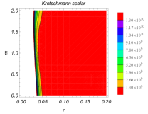
(a) $q_{M}=0.1$, $k=1$, $g(\varepsilon)=f(\varepsilon)=1.1$ and $\Lambda=-1$.

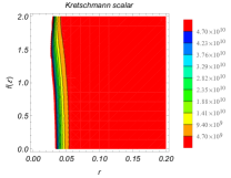
(b) $q_{M}=0.1$, $k=1$, $g(\varepsilon)=1.1$, $m=3$ and $\Lambda=-1$.

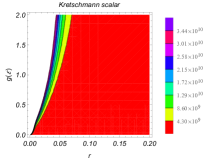
(c) $q_{M}=0.1$, $k=1$, $f(\varepsilon)=1.1$, $m=3$ and $\Lambda=-1$.

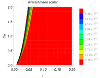
(d) $k=1$, $g(\varepsilon)=f(\varepsilon)=1.1$, $m=3$ and $\Lambda=-1$.

Figure 1: Variation of the $K$ as a function of different parameters for $q_{E}=0.1$.

If we keep the radial component ($r$) fixed, we find that: There is a specific geometrical mass $m_{s}$ where for $m<m_{s}$ the Kretschmann scalar is a decreasing function of this parameter, whereas for $m>m_{s}$, it becomes an increasing function of $m$. The same could be stated for energy functions and magnetic charge.

The asymptotic behavior of the Kretschmann scalar is obtained as

$$\lim_{r\longrightarrow\infty}K=-\frac{8\Lambda^{2}}{3}+O(\frac{1}{r^{6}}),$$

which shows that the asymptotic behavior of the solutions is $AdS/dS$. Also, we see that magnetic and electric charges have not affected the asymptotic behavior.

II.2.3 Roots of metric function

The existence of black hole is restricted to the presence of at least one event horizon for the solutions. The event horizons are where metric function vanishes. It is necessary, but not sufficient. $\frac{d\psi(r)}{dr}$ should be positive at the event horizon, too. Otherwise, it is Cauchy or cosmological horizon. Considering the parameters present in the metric function, the following cases could be pointed out:

I) $\Lambda=0$: In this case, the roots of metric function are obtained in the following form

$$\left.r(\psi(r)=0)\right|_{\Lambda=0}=\frac{m\pm\sqrt{m^{2}-4f^{2}(\varepsilon)kq_{E}^{2}-4g^{2}(\varepsilon)kq_{m}^{2}}}{2k}.$$ (15)

The first condition for existence of real positive valued roots for this case is given by

$$m^{2}\geq 4f^{2}(\varepsilon)kq_{E}^{2}+4g^{2}(\varepsilon)kq_{m}^{2},$$ (16)

which puts a lower limit on geometrical mass. If the mentioned condition is not satisfied, solutions suffer the absence of root and are interpreted as naked singularity. The positivity of the root is another condition that must be met. Considering this, one can confirm that for hyperbolic case, only one root could be observed. For spherical black holes, if $m^{2}=4f^{2}(\varepsilon)kq_{E}^{2}+4g^{2}(\varepsilon)kq_{m}^{2}$, solutions will have only one root, otherwise, there exist two roots for the metric function.

II) $m=0$: The roots of the metric function for this case are extracted as

$$\left.r(\psi(r)=0)\right|_{m=0}=\sqrt{\frac{3g^{2}(\varepsilon)k}{2\Lambda}\pm\frac{\sqrt{12f^{2}(\varepsilon)g^{2}(\varepsilon)\Lambda q_{E}^{2}+9g^{4}(\varepsilon)k^{2}+12g^{4}(\varepsilon)\Lambda q_{M}^{2}}}{2\Lambda}}.$$ (17)

Here, two conditions are required to be satisfied for having real valued root. The first one is

$$\Lambda\geq\frac{3g^{2}(\varepsilon)k}{4f^{2}(\varepsilon)q_{E}^{2}+4g^{2}(\varepsilon)q_{M}^{2}}.$$ (18)

Such condition is automatically satisfied for $dS$ solutions while for $AdS$ black holes, a restriction is imposed on the values of different parameters. It is possible to trace out the effects of electric and magnetic charges, and one of the energy functions on root of the metric function if $\Lambda=\frac{3g^{2}(\varepsilon)k}{4f^{2}(\varepsilon)\Lambda q_{E}^{2}+4g^{2}(\varepsilon)q_{M}^{2}}$. In this case, only one root will be available for the metric function and it belongs to black holes with hyperbolic horizon. The second condition for the existence of real valued root for the metric function is given by

$$\frac{3g^{2}(\varepsilon)k}{2\Lambda}\pm\frac{\sqrt{12f^{2}(\varepsilon)g^{2}(\varepsilon)\Lambda q_{E}^{2}+9g^{4}(\varepsilon)k^{2}+12g^{4}(\varepsilon)\Lambda q_{M}^{2}}}{2\Lambda}\geq 0.$$ (19)

III) $\Lambda=m=0$: Interestingly, in the absence of geometrical mass and cosmological constant, it is possible to obtain root for the metric function as

$$\left.r(\psi(r)=0)\right|_{\Lambda=m=0}=\sqrt{-\frac{f^{2}(\varepsilon)q_{E}^{2}+g^{2}(\varepsilon)q_{M}^{2}}{k}},$$ (20)

which shows that only solutions with hyperbolic horizon enjoy the existence of event horizon in their structures. It should be noted that root in this case is an increasing function of the electric and magnetic charges, and rainbow functions.

IV) General case: It is possible to obtain the root of metric function analytically for this case as

$$r(\psi(r)=0)=\sqrt{\frac{12a_{1}^{1/3}g(\varepsilon)^{2}k-(2a_{1})^{2/3}+18\sqrt[3]{2}g(\varepsilon)^{2}\left(4f(\varepsilon)^{2}\Lambda q_{E}^{2}-g(\varepsilon)^{2}\left(k^{2}-4\Lambda q_{M}^{2}\right)\right)}{24a_{1}^{1/3}\Lambda}}\pm\frac{\sqrt{a_{2}}}{2}$$ (21)

where

$$a_{1} = 27g(\varepsilon)^{4}\left(24f(\varepsilon)^{2}k\Lambda q_{E}^{2}+2g(\varepsilon)^{2}\left(k^{3}+12k\Lambda q_{M}^{2}\right)-9\Lambda m^{2}\right)+$$

$$\sqrt{729g(\varepsilon)^{8}\left(24f(\varepsilon)^{2}k\Lambda q_{E}^{2}+2g(\varepsilon)^{2}\left(k^{3}+12k\Lambda q_{M}^{2}\right)-9\Lambda m^{2}\right)^{2}-2916g(\varepsilon)^{6}\left(g(\varepsilon)^{2}\left(k^{2}-4\Lambda q_{M}^{2}\right)-4f^{2}\Lambda q_{E}^{2}\right)^{3}}$$

$$a_{2} = \frac{24a_{1}g(\varepsilon)^{2}k+2^{2/3}a_{1}^{2}+18\sqrt[3]{2}g(\varepsilon)^{2}\left(g(\varepsilon)^{2}\left(k^{2}-4\Lambda q_{M}^{2}\right)-4f(\varepsilon)^{2}\Lambda q_{E}^{2}\right)}{6a_{1}\Lambda}-$$

$$\frac{6\sqrt{6}g(\varepsilon)^{2}m}{\Lambda\sqrt{\frac{12a_{1}g(\varepsilon)^{2}k-2^{2/3}a_{1}^{2}+18\sqrt[3]{2}g(\varepsilon)^{2}\left(4f(\varepsilon)^{2}\Lambda q_{E}^{2}-g(\varepsilon)^{2}\left(k^{2}-4\Lambda q_{M}^{2}\right)\right)}{a_{1}\Lambda}}}$$

Apparently, under certain conditions, system could enjoy the existence of one of the following cases: two roots, one root and absence of root. The absence of root (naked singularity) takes place when the argument under square root functions is not positive valued. In order to understand the effects of different parameters on the number of the roots, we have plotted Fig. 2.

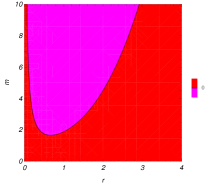
(a) $q_{M}=0.5$, $k=1$, $g(\varepsilon)=f(\varepsilon)=1.1$ and $\Lambda=-1$.

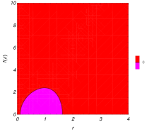
(b) $q_{M}=0.5$, $k=1$, $g(\varepsilon)=1.1$, $m=3$ and $\Lambda=-1$.

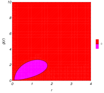
(c) $q_{M}=0.5$, $k=1$, $f(\varepsilon)=1.1$, $m=3$ and $\Lambda=-1$.

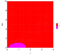
(d) $k=1$, $g(\varepsilon)=f(\varepsilon)=1.1$, $m=3$ and $\Lambda=-1$.

Figure 2: Variation of $\psi(r)$ as a function of different parameters for $q_{E}=0.5$

Evidently, for geometrical mass, there is a lower bound, $m_{bound}$ where for $m<m_{bound}$, metric function does not have a root and the singularity is naked. For $m=m_{bound}$ and $m>m_{bound}$ system will have one and two roots, respectively. The smaller (larger) root is a decreasing (increasing) function of geometrical mass. The effects of $f(\varepsilon)$ and $q_{M}$ on number of roots is similar. There is an upper bound on these parameters below which the system has roots. The larger (smaller) root is a decreasing (increasing) function of $f(\varepsilon)$ and $q_{M}$.

For $g(\varepsilon)$, we have also an upper bound. But interestingly, while the smaller root is always an increasing function of $g(\varepsilon)$, the larger root is first an increasing function of this parameter and then it becomes a decreasing function of it. The reason for this behavior is due to special coupling of $g(\varepsilon)$ with cosmological constant and magnetic charge (see Eq. 13). For specific range of $g(\varepsilon)$, the $\Lambda$ term is dominant in behavior of the larger root, while for the other range, the effects of magnetic charge term kicks in and becomes dominant. It should be noted that in the absence of the magnetic charge, such behavior would not be observed for variation of $g(\varepsilon)$. Therefore, this specific behavior for this energy function is due to the magnetic nature of the solutions.

So far, we established the fact that our solutions have an inherently irremovable singularity which could be covered by at least one horizon. This confirms that our solutions could be interpreted as black holes.

III Thermodynamics

In this section, we investigate the thermodynamical properties of our solutions. The main issue is to see how the presence of rainbow functions and their specific coupling with other parameters would modify the thermodynamical behavior of the solutions. Before we go on, we introduce a new notion for our solutions. We consider the negative cosmological constant to be a thermodynamical quantity known as pressure. Such a proposal was used by Kubiznak and Mann in Ref. Kubiznak to show the presence of van der Waals like behavior for black holes and since then, it has been widely used in literature. Therefore, from now on, we replace the cosmological constant with pressure using the following relation

$$\Lambda=-8\pi P.$$

It should be noted that replacing the cosmological constant with pressure results into modification of the first law of the black hole thermodynamics for these black holes as HRP ; Dutta

$$dM=TdS+VdP+\Phi_{E}dQ_{E}+\Phi_{M}dQ_{M},$$ (22)

where $Q_{E}$ and $Q_{M}$ are total electric and magnetic charges, $\Phi_{E}$ and $\Phi_{M}$ are electric and magnetic potentials, and $V$ is the thermodynamic volume of the black hole.

In what follows, first, we extract thermodynamical quantities and study their properties. Then, we investigate the possibility of van der Waals like phase transition for these black holes. Later on, we obtain conditions for thermal stability/instability. It should be noted that all of the thermodynamical quantities are calculated on the outer horizon of the black hole, $r_{+}$.

III.1 Thermodynamical quantities

III.1.1 Temperature

The first thermodynamical quantity of interest is temperature. According to the pioneering work of Hawking, the temperature of black holes is related to surface gravity by the following relation HawkingT

$$T=\frac{\kappa}{2\pi}.$$

Therefore, the task of obtaining the temperature is limited to calculation of the surface gravity. The surface gravity is given by

$$\kappa=\sqrt{-\frac{1}{2}\left(\nabla_{\mu}\chi_{\nu}\right)\left(\nabla^{\mu}\chi^{\nu}\right)},$$

where $\chi^{\nu}$ is the time-like Killing vector. The metric employed in this paper (5) admits a Killing vector for temporal coordinate in the form of $\chi=\partial_{t}$. Using this vector, temperature will be calculated as

$$T=\frac{g(\varepsilon)}{4\pi f(\varepsilon)}\left.\frac{df\left(r\right)}{dr}\right|_{r=r_{+}}=\frac{8\pi Pr_{+}^{4}-g^{2}(\varepsilon)\left(f^{2}(\varepsilon)q_{E}^{2}+g^{2}(\varepsilon)q_{M}^{2}-kr_{+}^{2}\right)}{4\pi f(\varepsilon)g(\varepsilon)r_{+}^{3}},$$ (23)

Evidently, the specific coupling between magnetic and electric charges with energy functions that was observed in metric function is also present in the temperature. Therefore, previous arguments regarding the effects of gravity’s rainbow in the metric function are also valid for the temperature. Interestingly, if the event horizon satisfies the following condition

$$f^{2}(\varepsilon)q_{E}^{2}+g^{2}(\varepsilon)q_{M}^{2}-kr_{+}^{2}=0,$$ (24)

the temperature reduces to

$$T_{S}=\frac{2P}{f(\varepsilon)g(\varepsilon)}\sqrt{\frac{f^{2}(\varepsilon)q_{E}^{2}+g^{2}(\varepsilon)q_{m}^{2}}{k}},$$ (25)

indicating a fixed temperature independent of horizon radius of the black holes. Such temperature could only be real positive valued for black holes with spherical horizon and it is linearly related to the pressure. In addition, this temperature is a decreasing function of rainbow functions and an increasing function of magnetic and electric charges. For more clarification, we have plotted following diagrams (Fig. 3) for this specific temperature.

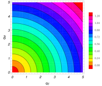
(a) $g(\varepsilon)=f(\varepsilon)=1.1$.

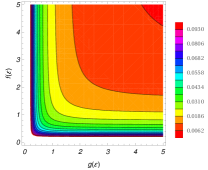
(b) $q_{M}=q_{E}=0.1$.

Figure 3: Variation of the $T_{S}$ as a function of different parameters for $k=1$ and $P=0.1.$

The value of horizon radius determines in which regime we are working. The high energy limit of the temperature is

$$\lim_{r_{+}\longrightarrow 0}T=-\frac{g^{3}(\varepsilon)q_{M}^{2}+g(\varepsilon)f^{2}(\varepsilon)q_{E}^{2}}{4\pi f(\varepsilon)r_{+}^{3}}+\frac{g(\varepsilon)k}{4\pi f(\varepsilon)r_{+}}+O(r_{+}),$$

whereas the asymptotic behavior is described by the following relation

$$\lim_{r_{+}\longrightarrow\infty}T=\frac{2Pr_{+}}{f(\varepsilon)g(\varepsilon)}+O(\frac{1}{r_{+}}).$$

The high energy limit is governed by rainbow function, electric and magnetic charges whereas the asymptotic behavior is determined by both the pressure and rainbow functions. The difference in signature of these two limits indicates that temperature has at least one root. Calculations show that temperature could have up to two roots given by

$$\left.r_{+}\right|_{T=0}=\sqrt{-\frac{g^{2}(\varepsilon)k}{16\pi P}\pm\frac{g(\varepsilon)\sqrt{32\pi P\left(f^{2}(\varepsilon)q_{E}^{2}+g^{2}(\varepsilon)q_{M}^{2}\right)+g^{2}(\varepsilon)k^{2}}}{16\pi P}}.$$ (26)

For spherical and flat horizon black holes, only positive branch results into real valued root for temperature. Therefore, for these two horizons, temperature has only one root. For black holes with hyperbolic horizon, although it seems that they could have two roots, their temperature has only one root. This is because the second term in the root of the temperature has higher value than the first term. Therefore, only the positive branch results into real valued root for the temperature. Considering the number of roots, high energy limit and asymptotic behavior, one can conclude that: the temperature has a root. At this root, temperature changes sign from negative to positive. In classical thermodynamic of black holes, positivity of temperature is considered as one of the criteria for having physical solutions. Therefore, before the temperature’s root, solutions are non-physical and the root of temperature is providing us with a lower bound. Later (in section III.2), we will show that roots of the temperature and heat capacity are identical and will show how these roots will be modified as a function of different parameters.

The gravity’s rainbow has noticeable effects on the temperature. In high energy regime, rainbow functions affect the thermodynamical behavior of the temperature differently compared to asymptotic behavior. In asymptotic limit, the rainbow functions have identical effects on temperature. In high energy limit, the situation is different. This difference in behavior is due to the presence of the magnetic charge and its coupling with rainbow functions which is different from the electric charge. In section III.3, we will point out that the temperature could exhibit a van der Waals like behavior and phase transition. It should be noted that obtained temperature coincides with $(\frac{dM}{dS})_{Q_{E},Q_{M},P}$ taken from the first law of black hole thermodynamics (22).

III.1.2 Entropy

The method for obtaining the entropy of black holes depends on gravities under consideration and topological structure of the black holes. For topological black holes in the presence of Einstein gravity, the area law proposed by Hawking and Bekenstein is a valid method for calculating entropy Beckenstein ; Hawking . Therefore, considering the metric (5), the entropy can be calculated by

$$S=\frac{1}{4}\int d^{2}x\sqrt{\gamma}=\frac{1}{4g^{2}(\varepsilon)}r_{+}^{2},$$ (27)

in which $\gamma_{ab}$ is the induced metric on the $2$-dimensional boundary. The entropy is a smooth increasing function of the horizon radius and a decreasing function of only one of the rainbow functions. The dependency of entropy on only one of the rainbow functions is due to coupling of it with spatial coordinates (see Eq. (5)). If one considers the condition (24) (which resulted into a fixed temperature (25)), a fixed entropy will be obtained as

$$S_{S}=\frac{f^{2}(\varepsilon)q_{E}^{2}+g^{2}(\varepsilon)q_{m}^{2}}{4kg^{2}(\varepsilon)},$$ (28)

which has the following interesting properties. First of all, the non-negative entropy could only be obtained for black holes with spherical horizon ($k>0$). In addition, this entropy is expressed in term of the matter field and rainbow functions. It is an increasing function of the $f(\varepsilon)$, electric and magnetic charges and a decreasing function of $g(\varepsilon)$.

III.1.3 Mass

The mass of black holes, without replacing cosmological constant with pressure in it, is depicted as internal energy. By inserting the cosmological constant as pressure, the role of the mass is changed to enthalpy. There are several methods for calculating the mass. One of them is employing Hamiltonian approach. The other method is using counterterm method. Both of these methods result into a general form for mass expressed as

$$M=\frac{f(\varepsilon)}{8\pi g(\varepsilon)}m.$$

Evaluating the metric function on horizon ($f(r=r_{+})=0$), solving it with respect to geometrical mass and replacing cosmological constant with pressure result into the following relation for total mass of these black holes

$$M=\frac{8\pi Pr_{+}^{4}+3g^{2}\left(f^{2}(\varepsilon)q_{E}^{2}+g^{2}(\varepsilon)q_{M}^{2}+kr_{+}^{2}\right)}{24\pi f(\varepsilon)g^{3}(\varepsilon)r_{+}}.$$ (29)

Evidently, the mass is an increasing function of the pressure, rainbow functions, electric and magnetic charges. The only term that could have negative effect on the value of the mass is topological term. To understand the effects of different parameters on the mass, we study the high energy and asymptotic limits. The high energy limit of the mass is

$$\lim_{r_{+}\longrightarrow 0}M=\frac{g^{2}(\varepsilon)q_{M}^{2}+f^{2}(\varepsilon)q_{E}^{2}}{8\pi f(\varepsilon)g(\varepsilon)r_{+}}+\frac{kr_{+}}{8\pi f(\varepsilon)g(\varepsilon)}+O(r_{+}),$$

whereas the asymptotic behavior is described by the following relation

$$\lim_{r_{+}\longrightarrow\infty}M=\frac{Pr_{+}^{3}}{3f(\varepsilon)g^{3}(\varepsilon)}+\frac{kr_{+}}{8\pi f(\varepsilon)g(\varepsilon)}+O(\frac{1}{r_{+}}).$$

For small black holes, this is the matter field (electric and magnetic charges) that has dominant effect on the behavior of mass. Contrary to what was observed for temperature, the high energy limit of mass is positive valued and an increasing function of the rainbow functions, electric and magnetic charges. On the other hand, the asymptotic behavior of mass, similar to temperature, is positive valued, dominated by pressure and it is a decreasing function of rainbow functions. For medium black holes, the dominant term in the behavior of mass is the topological term. This term could be negative for hyperbolic horizon while it is positive for spherical and horizon flat black holes. Therefore, the mass is positive valued without any root for arbitrary horizon radius in case of spherical and horizon flat black holes. Whereas, for hyperbolic black holes, mass could be negative valued and acquires roots. The roots of mass are given by

$$\left.r_{+}\right|_{M=0}=\sqrt{-\frac{3g^{2}(\varepsilon)k}{16\pi P}\pm\frac{g(\varepsilon)\sqrt{9g^{2}(\varepsilon)k^{2}-96\pi P\left(f^{2}(\varepsilon)q_{E}^{2}+g^{2}(\varepsilon)q_{M}^{2}\right)}}{16\pi P}},$$

which are pretty similar to the roots obtained for temperature. Therefore, the same arguments stated for having real valued roots for temperature is also valid here. It should be noted that according to the first law of the black hole thermodynamics (22), the roots of temperature are actually where mass acquires extremum. Remembering that temperature could acquire only one root, mass could have up to one extremum. Considering the high energy limit and asymptotic behavior of the mass, one can safely conclude that extremum is a minimum. This indicates that mass has a lower limit on values that it can take. In addition, depending on the place of this minimum, mass could have up to two roots with a region of negativity. To show this, we have plotted Fig. 3.

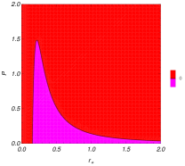
(a) $q_{M}=0.1$ and $g(\varepsilon)=f(\varepsilon)=1.1$.

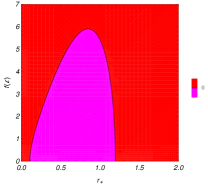
(b) $q_{M}=P=0.1$ and $g(\varepsilon)=1.1$.

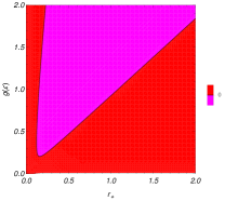
(c) $q_{M}=P=0.1$ and $f(\varepsilon)=1.1$.

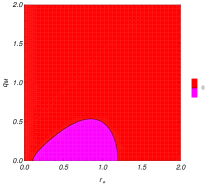
(d) $P=0.1$ and $g(\varepsilon)=f(\varepsilon)=1.1$.

Figure 4: Variation of the $M$ as a function of different parameters for $q_{E}=0.1$ and $k=-1$

If we consider the positivity of mass as a condition for having physical solutions, one can conclude that for black holes with hyperbolic horizon, the mass is bounded. In other words, for specific regions, no physical solutions exist for black holes due to negativity of the mass. According to Fig. 4, the region of negativity for mass is an increasing function of the $g(\varepsilon)$ while it is a decreasing function of the $f(\varepsilon)$, pressure and magnetic charge. As one can see, both smaller and larger roots of mass are increasing functions of $g(\varepsilon)$. Whereas, larger (smaller) root is a decreasing (increasing) function of $f(\varepsilon)$, pressure and magnetic charge. It should be noted that energy functions have opposite effective behavior on mass but their effectiveness is different. One can find that the effect of $g(\varepsilon)$ on mass is more significant than $f(\varepsilon)$. Once more, we remind the reader that $g(\varepsilon)$ is coupled with spatial coordinates while $f(\varepsilon)$ is coupled with temporal coordinate. Considering this, one can also state that mass is more affected by spatial coordinate comparing to temporal coordinate of the metric.

III.1.4 Pressure

Our next thermodynamical quantity of interest is pressure. Replacing the cosmological constant with pressure changes the type of the relation which was obtained for pressure. After replacement, this relation becomes actually the equation of state. Therefore, using the temperature (23), one can obtain the pressure in the following form

$$P=\frac{4\pi g(\varepsilon)f(\varepsilon)r_{+}^{3}T+g^{2}(\varepsilon)\left(f^{2}(\varepsilon)q_{E}^{2}+g^{2}(\varepsilon)q_{M}^{2}-kr_{+}^{2}\right)}{8\pi r_{+}^{4}}.$$ (30)

The first noticeable issue is the fact that there is no energy function in the denominator of this relation for pressure. This is in contrast of what was observed for previously calculated thermodynamical quantities (see Eqs. (23), (27) and (29)). Therefore, if black holes have hyperbolic horizon, the pressure will be an increasing function of the rainbow functions, temperature, electric and magnetic charges. For spherical black holes, the topological term in pressure negatively affects it. To have a better understanding of the pressure’s properties, we investigate the high energy limit given by

$$\lim_{r_{+}\longrightarrow 0}P=\frac{g^{4}(\varepsilon)q_{M}^{2}+g^{2}(\varepsilon)f^{2}(\varepsilon)q_{E}^{2}}{8\pi r_{+}^{4}}-\frac{kg^{2}(\varepsilon)}{8\pi r_{+}^{2}}+O(r_{+}),$$

and asymptotic behavior obtained by

$$\lim_{r_{+}\longrightarrow\infty}P=\frac{g(\varepsilon)f(\varepsilon)T}{2r_{+}}-\frac{kg^{2}(\varepsilon)}{8\pi r_{+}^{2}}+O(\frac{1}{r_{+}}).$$

Evidently, the dominant factors for small, medium and large black holes are matter field (electric and magnetic charges), topological term and temperature, respectively. The topological term for hyperbolic and horizon flat black holes is positive. Therefore, in these two cases, pressure is positive everywhere and it has no root. For spherical black holes, since the topological term is negative, the pressure could acquire root given by

$$\left.r_{+}\right|_{P=0}=\left\{\begin{array}[]{c}\frac{g(\varepsilon)^{2}k^{2}+a_{3}^{2/3}+g(\varepsilon)k\sqrt[3]{a_{3}}}{12\sqrt[3]{a_{3}}\pi f(\varepsilon)T},\\ \\ \frac{4g(\varepsilon)k\sqrt[3]{a_{3}}\pm 2i\left(\sqrt{3}\pm i\right)g(\varepsilon)^{2}k^{2}-2\left(1\pm i\sqrt{3}\right)a_{3}^{2/3}}{48\sqrt[3]{a_{3}}\pi f(\varepsilon)T},\end{array}\right.$$

where

$$a_{3}=g(\varepsilon)^{3}k^{3}-216\pi^{2}f(\varepsilon)^{2}g(\varepsilon)T^{2}\left(f(\varepsilon)^{2}q_{E}^{2}+g(\varepsilon)^{2}q_{M}^{2}\right)+\frac{1}{2}\sqrt{\left(2g(\varepsilon)^{3}k^{3}-432\pi^{2}f(\varepsilon)^{2}g(\varepsilon)T^{2}\left(f(\varepsilon)^{2}q_{E}^{2}+g^{2}q_{M}^{2}\right)\right)^{2}-4g(\varepsilon)^{6}k^{6}}.$$

The effects of different parameters on the number of roots and negativity/positivity of the pressure is investigated through Fig. 5.

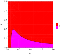
(a) $q_{M}=0.1$ and $g(\varepsilon)=f(\varepsilon)=1.1$.

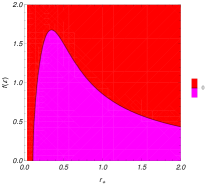
(b) $q_{M}=T=0.1$ and $g(\varepsilon)=1.1$.

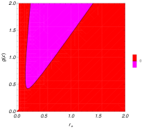
(c) $q_{M}=T=0.1$ and $f(\varepsilon)=1.1$.

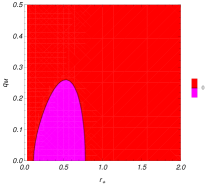
(d) $T=0.1$ and $g(\varepsilon)=f(\varepsilon)=1.1$.

Figure 5: Variation of the $P$ as a function of different parameters for $q_{E}=0.1$ and $k=1$.

The negative pressure is not physically acceptable in the context of black hole thermodynamics. In addition, the plotted diagrams for pressure are similar to those plotted for the mass (compare Fig. 5 with Fig. 4). Therefore, the effects of different parameters on the behavior of the pressure is similar to those discussed for the mass. It should be noted that pressure enjoys up to two roots. Using the concept of first law of black hole thermodynamics (22) with the obtained mass (29), one can obtain the volume of these black holes as

$$V=(\frac{dM}{dP})_{q_{M},q_{E}}=\frac{r_{+}^{3}}{3g^{3}(\varepsilon)f(\varepsilon)},$$ (31)

which shows that total volume is linearly related to the horizon radius. Therefore, one can use horizon radius instead of volume for describing different phenomena and calculations. The volume is a decreasing function of both rainbow functions. If we compare the obtained volume (31) with entropy (27), we see that they are related with the following relation

$$S=\frac{3g^{3}(\varepsilon)f(\varepsilon)}{4r_{+}}V.$$

In fact, this is expected. The reason is that entropy is calculated by using the area of the black holes. Therefore, the obtained volume divide by $r_{+}$ has sound relation with area of the black holes. The main issue is the dependency of the volume on both of the rainbow functions. Both of them are in denominator of the volume but the effect of rainbow function coupled with spatial coordinate is more significant compared to the one coupled with temporal coordinate.

According to conventional thermodynamic, the pressure is a decreasing function of the volume. In any place that such principle is violated, that region is not physically accessible for the thermodynamical system and phase transition could take place. If we apply the thermodynamical principle to black holes, we expect the pressure to be a decreasing function of the horizon radius (volume). The high energy limit (which diverges for $r_{+}=0$) and asymptotic behavior (which goes to zero for $r\longrightarrow\infty$) show that the mentioned principle is satisfied for small and large black holes. The remaining is the medium black holes. In order to see whether pressure is a decreasing/increasing function of the horizon radius, we calculate the first order derivation of the pressure with respect to horizon radius

$$(\frac{dP}{dr_{+}})_{q_{M},q_{E},T}=-\frac{2\pi g(\varepsilon)f(\varepsilon)r_{+}^{3}T+g^{2}(\varepsilon)\left(f^{2}(\varepsilon)q_{E}^{2}+g^{2}(\varepsilon)q_{M}^{2}-kr_{+}^{2}\right)}{4\pi r_{+}^{5}}.$$

For hyperbolic and flat horizons, this expression is negative, therefore, one can conclude that black holes for these horizons also admit the mentioned principle. For the spherical black holes, the situation is different. In this case, such expression could become positive valued violating the principle. To express such possibility, we have plotted diagrams in Fig. 6.

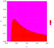
(a) $q_{M}=0.1$ and $g(\varepsilon)=f(\varepsilon)=1.1$.

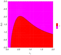
(b) $q_{M}=T=0.1$ and $g(\varepsilon)=1.1$.

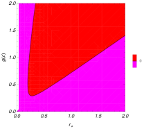
(c) $q_{M}=T=0.1$ and $f(\varepsilon)=1.1$.

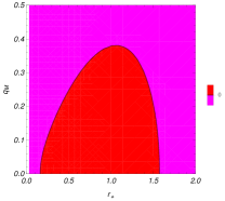
(d) $T=0.1$ and $g(\varepsilon)=f(\varepsilon)=1.1$.

Figure 6: Variation of the $(\frac{dP}{dr_{+}})_{q_{M},q_{E},T}$ as a function of different parameters for $q_{E}=0.1$ and $k=1$.

Accordingly, one can point to the existence of specific values for temperature ($T_{S}$), magnetic charge ($q_{M_{S}}$) and $f(\varepsilon)$ ($f(\varepsilon)_{S}$) where for values smaller than them, pressure will acquire a region of negativity. For $g(\varepsilon)$, in contrast, there is special energy function, $g(\varepsilon)_{S}$, where for values larger than that, pressure will have a region of negativity. That being said, one can conclude that the region of negativity for pressure is a decreasing function of temperature, magnetic charge and $f(\varepsilon)$ while it is an increasing function of $g(\varepsilon)$. It should be noted that places where signature of the $(\frac{dP}{dr_{+}})_{q_{M},q_{E},T}$ changes are where pressure meets an extremum. Therefore, pressure can have up to two extrema. Considering the high energy and asymptotic behaviors of the pressure, one can state that the smaller extremum is a minimum and larger one is a maximum. The region between such extrema is not physical, so there is a phase transition taking place over this region. In section III.3, we will address the type of the phase transition that was observed here and investigate the pressure in more details.

III.1.5 Gibbs free energy

The Gibbs free energy is a potential that can be used to determine the equilibrium point at constant pressure and temperature in the processes that a thermodynamical system goes through. At this equilibrium point, the Gibbs free energy is minimized. Considering that we are working in extended phase space, one can use the following relation to obtain the Gibbs free energy for these black holes

$$G=H-TS=M-TS=\frac{3g^{2}(\varepsilon)\left(3f^{2}(\varepsilon)q_{E}^{2}+3g^{2}(\varepsilon)q_{M}^{2}+kr_{+}^{2}\right)-8\pi Pr_{+}^{4}}{48\pi f(\varepsilon)g^{3}(\varepsilon)r_{+}}.$$ (32)

Contrary to temperature (23) and mass (29), Gibbs free energy is a decreasing function of the pressure. In addition, it is an increasing function of the electric and magnetic charges, and the effects of topological term depends on the horizon. For spherical and flat horizons, the topological term positively affect the Gibbs free energy, while the opposite stands for black holes with hyperbolic horizon.

The high energy limit of the Gibbs free energy is given by

$$\lim_{r_{+}\longrightarrow 0}G=\frac{3(g^{2}(\varepsilon)q_{M}^{2}+f^{2}(\varepsilon)q_{E}^{2})}{16\pi f(\varepsilon)g(\varepsilon)r_{+}}+\frac{kr_{+}}{16\pi f(\varepsilon)g(\varepsilon)}+O(r_{+}),$$

while the asymptotic behavior is

$$\lim_{r_{+}\longrightarrow\infty}G=-\frac{Pr_{+}^{3}}{6f(\varepsilon)g^{3}(\varepsilon)}+\frac{kr_{+}}{16\pi f(\varepsilon)g(\varepsilon)}+O(\frac{1}{r_{+}}).$$

The high energy limit of the Gibbs free energy is positive valued while the asymptotic behavior is negative valued. Considering this, one can conclude that at least one root exists for Gibbs free energy. The medium black holes are governed by topological term. It is a matter of calculation to show that Gibbs free energy could have up to two roots given by

$$\left.r_{+}\right|_{G=0}=\sqrt{\frac{3g^{2}(\varepsilon)k}{16\pi P}\pm\frac{3g(\varepsilon)\sqrt{32\pi P\left(f^{2}(\varepsilon)q_{E}^{2}+g^{2}(\varepsilon)q_{M}^{2}\right)+g^{2}(\varepsilon)k^{2}}}{16\pi P}}.$$

Considering the application of Gibbs free energy to determine the equilibrium point, the first order derivation of it with respect to horizon radius (volume) is obtained by

$$(\frac{dG}{dr_{+}})_{q_{M},q_{E},T,P}=-\frac{g^{2}(\varepsilon)\left(3f^{2}(\varepsilon)q_{E}^{2}+3g^{2}(\varepsilon)q_{M}^{2}-kr_{+}^{2}\right)+8\pi Pr_{+}^{4}}{16\pi f(\varepsilon)g^{3}(\varepsilon)r_{+}^{2}}.$$

The pressure, magnetic and electric charge terms enjoy the same sign whereas the topological term has an opposite sign. Considering this, for flat and hyperbolic horizons, the Gibbs free energy will be without any extremum, whereas the spherical black holes could enjoy at least one extremum in their Gibbs free energy. Considering this, one can extract extrema points in the following form

$$\left.r_{+}\right|_{(\frac{dG}{dr_{+}})=0}=\sqrt{\frac{g^{2}(\varepsilon)k}{16\pi P}\pm\frac{g(\varepsilon)\sqrt{g^{2}(\varepsilon)k^{2}-96\pi P\left(f^{2}(\varepsilon)q_{E}^{2}+g^{2}(\varepsilon)q_{M}^{2}\right)}}{16\pi P}}.$$ (33)

Evidently, the Gibbs free energy for spherical black holes ($k=1$) could enjoy up to two extrema. Considering the high energy limit and asymptotic behavior of the Gibbs free energy, if there are two extrema for it, the first extremum will be a minimum while the second one is a maximum. In order to elaborate this fact and investigate the effects of different parameters on these extrema, we have plotted Fig. 7.

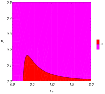
(a) $q_{M}=0.1$ and $g(\varepsilon)=f(\varepsilon)=1.1$.

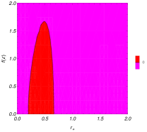
(b) $q_{M}=P=0.1$ and $g(\varepsilon)=1.1$.

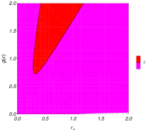
(c) $q_{M}=P=0.1$ and $f(\varepsilon)=1.1$.

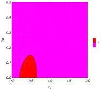
(d) $P=0.1$ and $g(\varepsilon)=f(\varepsilon)=1.1$.

Figure 7: Variation of the $(\frac{dG}{dr_{+}})_{q_{M},q_{E},T,P}$ as a function of different parameters for $q_{E}=0.1$ and $k=1$.

The plotted diagrams for $(\frac{dG}{dr_{+}})_{q_{M},q_{E},T,P}$ are similar to those that were obtained for $(\frac{dP}{dr_{+}})_{q_{M},q_{E},T}$ indicating that the effects of the rainbow functions and magnetic charge are same as those that were reported before. The minimum (maximum) is an increasing (decreasing) function of the pressure, magnetic charge and $f(\varepsilon)$ whereas, both the maximum and minimum are increasing functions of $g(\varepsilon)$.

The existence of equilibrium point indicates that there is at least two distinguishable phases available for the thermodynamical system. In fact, the equilibrium point is where two phases meet and phase transition could take place between them. The Gibbs free energy should be a decreasing function of the volume. Considering this, the region between two extrema, where Gibbs free energy becomes an increasing function of the volume (horizon radius) is not physically acceptable. Therefore, this region is not accessible for the black holes and there is a phase transition over this region for different phases available for the black holes. Once more, we point out that rainbow functions have opposite effects on these two properties of the Gibbs free energy. Later (in section III.3), we will investigate the type of phase transition.

III.1.6 Electric and magnetic properties

The total electric and magnetic charges of a system could be calculated by Gauss law. Using this law, one can show that the total electric and magnetic charges could be obtained as

$$Q_{E}=\frac{f(\varepsilon)q_{E}}{4\pi g(\varepsilon)},$$ (34)

$$Q_{M}=\frac{f(\varepsilon)q_{M}}{4\pi g(\varepsilon)},$$ (35)

which show that due to the contribution of the gravity’s rainbow, the total electric and magnetic charges are modified. This is in contrast to what were observed for Gauss-Bonnet GB , dilatonic gravities Dilaton and Born-Infeld nonlinear electrodynamic generalization Dilaton .

To obtain the electric and magnetic fields, we use the first law of black hole thermodynamics. We employ (22) to obtain these quantities which results into

$$\Phi_{E}=(\frac{dM}{dQ_{E}})_{P,S,Q_{M}}=\frac{q_{E}}{r_{+}},$$ (36)

$$\Phi_{M}=(\frac{dM}{dQ_{M}})_{P,S,Q_{E}}=\frac{f^{2}(\varepsilon)q_{M}}{g^{2}(\varepsilon)}.$$ (37)

The obtained electric field matches the one that was calculated before for electrically charged black holes in the presence of gravity’s rainbow GB ; Dilaton . It is independent of the rainbow functions. Interestingly and contrary to electric field, the magnetic field is dependent of the rainbow functions and is affected by generalization of the rainbow gravity. But it should be noted that the rainbow functions have opposite effects on this quantity and if we choose the rainbow functions to be identical, the effects of gravity’s rainbow on this quantity will be removed.

III.2 Stability of the solutions

In canonical ensemble, the thermal stability of the black hole is determined by the behavior of heat capacity. The signature of the heat capacity is a tool that is used for determining thermal stability/instability of black holes. In previous sections, we showed that these black holes enjoy more than one phase in their thermodynamical state. Here, using the heat capacity, we determine the number of the phases available for the black holes and their thermal stability. It is worthwhile to mention that a black hole is thermally stable (unstable) if its heat capacity is positive (negative). In addition, the discontinuities in heat capacity could be interpreted as phase transition points.

The heat capacity for black holes under consideration is given by

$$C=T\frac{(\frac{dS}{dr_{+}})_{q_{M},q_{E},P}}{(\frac{dT}{dr_{+}})_{q_{M},q_{E},P}}=\frac{r_{+}^{2}(8\pi Pr_{+}^{4}-g^{2}(\varepsilon)\left(f^{2}(\varepsilon)q_{E}^{2}+g^{2}(\varepsilon)q_{M}^{2}-kr_{+}^{2}\right))}{16\pi g^{2}(\varepsilon)Pr_{+}^{4}+2g^{4}(\varepsilon)\left(3f^{2}(\varepsilon)q_{E}^{2}+3g^{2}(\varepsilon)q_{M}^{2}-kr_{+}^{2}\right)}.$$ (38)

The first noticeable issue is that the sign of the topological, electric and magnetic terms is different in numerator and denominator of heat capacity. While in the numerator, mentioned terms are coupled with horizon radius with higher power, in the denominator, they are coupled with higher power of $g(\varepsilon)$. The same coupling also takes place for the pressure term where its sign is identical in both numerator and denominator of the heat capacity. Remembering the role of heat capacity’s sign and its divergencies on determining the number of phases, we extract its roots in the following form

$$\left.r_{+}\right|_{C=0}=\sqrt{-\frac{g^{2}(\varepsilon)k}{16\pi P}\pm\frac{g(\varepsilon)\sqrt{32\pi P\left(f^{2}(\varepsilon)q_{E}^{2}+g^{2}(\varepsilon)q_{M}^{2}\right)+g^{2}(\varepsilon)k^{2}}}{16\pi P}}.$$ (39)

while the divergencies are obtained by

$$\left.r_{+}\right|_{C\longrightarrow\infty}=\sqrt{\frac{g^{2}(\varepsilon)k}{16\pi P}\pm\frac{g(\varepsilon)\sqrt{g^{2}(\varepsilon)k^{2}-96\pi P\left(f^{2}(\varepsilon)q_{E}^{2}+g^{2}(\varepsilon)q_{M}^{2}\right)}}{16\pi P}}.$$ (40)

The obtained roots for heat capacity (39) coincide with those extracted from temperature (26). Therefore, the heat capacity and temperature share the same root. On the other hand, the divergencies of heat capacity are identical to the extrema extracted for $(\frac{dG}{dr_{+}})_{q_{M},q_{E},T,P}$. In previous sections, we established that the range between roots of $(\frac{dG}{dr_{+}})_{q_{M},q_{E},T,P}$ is actually an inaccessible region for the black holes. In addition, we pointed out that such region and roots (which were equilibrium points) could only be observed for black holes with spherical horizon. Therefore, here as well, one can conclude that only for spherical black holes, existence of two divergencies for these black holes could be observed.

The number of phases present in the thermodynamical state of the black holes depends on number of roots and divergencies. In previous section, we pointed out that these black holes could enjoy up to one root in their temperature. Therefore, heat capacity has only one root. On the other hand, we pointed out that depending on values of different parameters, spherical black holes could have up to two roots for $(\frac{dG}{dr_{+}})_{q_{M},q_{E},T,P}$ and black holes with flat and hyperbolic horizons have no such roots. Therefore, one can also conclude that heat capacity for spherical black holes could have up to two divergencies, otherwise, there is no divergency for black holes. To make more clarification, we have plotted Fig. 8 for variation of heat capacity as a function of different parameters.

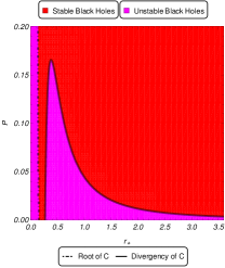
(a) $q_{M}=0.1$, $k=1$ and $g(\varepsilon)=f(\varepsilon)=1.1$.

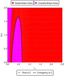
(b) $q_{M}=P=0.1$, $k=1$ and $g(\varepsilon)=1.1$.

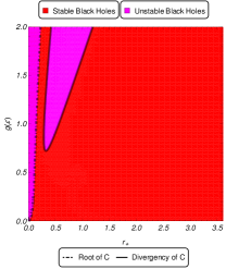
(c) $q_{M}=P=0.1$, $k=1$ and $f(\varepsilon)=1.1$.

(d) $P=0.1$, $k=1$ and $g(\varepsilon)=f(\varepsilon)=1.1$.

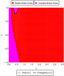
(e) $q_{M}=P=0.1$ and $g(\varepsilon)=f(\varepsilon)=1.1$.

Figure 8: Variation of the $C$ as a function of different parameters for $q_{E}=0.1$.

As it was pointed out, the heat capacity has only up to one root. The place of this root is an increasing function of the rainbow functions and magnetic charge, a decreasing function of the topological factor and not significantly affected by pressure. The number of divergencies in heat capacity is a decreasing function of the pressure, magnetic charge and $f(\varepsilon)$ while it is an increasing function of $g(\varepsilon)$ and topological factor. In other words, the region between two divergencies is a decreasing function of the pressure, magnetic charge and $f(\varepsilon)$ and an increasing function $g(\varepsilon)$ and topological factor.

Considering the effects of different parameters, the possible scenarios regarding the number of phases for these black holes are the following ones:

I) One root: there are two phases of small and large black holes. The small one has negative temperature and therefore, not physical. Whereas, the large black hole phase is thermally stable.

II) One root and one divergency: In this case, we have three phases of small, medium and large black holes. The small black holes are not physical due to negativity of the temperature. The medium and large phase are separated by a divergence point. This divergency is actually the equilibrium point that was discussed in section III.1.5. Therefore, this is the point where two phases of medium and large black holes are in equilibrium and going from one to the other could be achieved via a critical process.

III) One root and two divergencies: In this case, we have four distinguishable phases for black holes; very small, small, medium and large black holes. Since the temperature is negative in the very small black hole phase, this phase is not a physical one. For small and large black hole phases, heat capacity and temperature are positive, Gibbs free energy and pressure have reasonable behaviors and mass is not negative. Therefore, these two phases satisfy the thermodynamical principle. For the medium black hole phase, although it has positive temperature and mass, the behaviors of Gibbs free energy and pressure violate thermodynamically expected behaviors and heat capacity is negative. Therefore, this phase is not physical and accessible for the black holes. The small, medium and large black hole phases are separated by two divergencies. This indicates that upon meeting these divergencies, system go through a phase transition between them and changes from small to larger black hole phases or vice versa.

Finally, we should point out that super magnetized and/or super pressurized black holes admit only two phases in their thermodynamical structure where they are separated by a root and only one of the phases is physical. Therefore, there is no phase transition for black holes in this case. The situation for rainbow functions is different. As we pointed out, the effects of energy functions on the number of the phases and divergencies of heat capacity (phase transitions) are opposite. While the number of phases and phase transition points are decreasing functions of $f(\varepsilon)$, they are increasing functions of $g(\varepsilon)$. The $f(\varepsilon)$ represents the effects of temporal coordinate while $g(\varepsilon)$ represents the effects of spatial coordinate. Considering this, one can conclude that effective behavior of the temporal coordinate is toward omitting phase transitions and instabilities in the system and acquiring a uniform stable state while the opposite is true for spatial coordinates.

To complete our discussions here, we investigate the high energy limit of heat capacity given by

$$\lim_{r_{+}\longrightarrow 0}C=-\frac{r_{+}^{2}}{6g^{2}(\varepsilon)}+\frac{kr_{+}^{4}}{9g^{2}(\varepsilon)(g^{2}(\varepsilon)q_{M}^{2}+f^{2}(\varepsilon)q_{E}^{2})}+O(r_{+}),$$

and asymptotic behavior obtained as

$$\lim_{r_{+}\longrightarrow\infty}C=\frac{r_{+}^{2}}{2g^{2}(\varepsilon)}+\frac{k}{8\pi P}+O(\frac{1}{r_{+}}).$$

Interestingly, contrary to other thermodynamical quantities, the high energy limit and asymptotic behavior of the heat capacity are only governed by horizon radius and one of the energy functions, $g(\varepsilon)$. The effect of topological structure becomes noticeable in the second dominant term of both limits.

III.3 van der Waals like Behavior

In the last section, we established the possibility of existence of thermodynamical phase transition for our solutions. We also pointed out the number of thermodynamical phases present for different cases. In this section, we would like to address the type of phase transition. To do so, we first extract critical values for different thermodynamical quantities and plot the corresponding diagrams to investigate the critical behavior of these thermodynamical quantities. To do so, we use the equation of state (30) and the properties of inflection point. Considering the relation between volume and horizon radius, the properties of inflection point could be extracted from

$$\left(\frac{\partial P}{\partial r_{+}}\right)_{T,q_{M},q_{E}}=\left(\frac{\partial^{2}P}{\partial r_{+}^{2}}\right)_{T,q_{M},q_{E}}=0,$$ (41)

which results into the following equation for obtaining critical horizon radius (volume)

$$6(f^{2}(\varepsilon)q_{E}^{2}+g^{2}(\varepsilon)q_{M}^{2})-kr_{+}^{2}=0.$$ (42)

Evidently, only for spherical black holes, one can obtain critical horizon radius, hence critical behavior. It is a matter of calculation to show that critical horizon radius, temperature, pressure and Gibbs free energy are given by

$$r_{c} = \sqrt{\frac{6(f^{2}(\varepsilon)q_{E}^{2}+g^{2}(\varepsilon)q_{M}^{2})}{k}},$$ (43)

$$T_{c} = \frac{g^{2}(\varepsilon)k^{\frac{3}{2}}}{3\pi f(\varepsilon)\sqrt{6(f^{2}(\varepsilon)q_{E}^{2}+g^{2}(\varepsilon)q_{M}^{2})}},$$ (44)

$$P_{c} = \frac{g(\varepsilon)k^{2}}{96\pi(f^{2}(\varepsilon)q_{E}^{2}+g^{2}(\varepsilon)q_{M}^{2})},$$ (45)

$$G_{c} = \frac{\sqrt{k(f^{2}(\varepsilon)q_{E}^{2}+g^{2}(\varepsilon)q_{M}^{2})}}{2\sqrt{6}\pi f(\varepsilon)2(\varepsilon)},$$ (46)

The obtained critical values also confirm that the critical behavior is only possible for spherical black holes while it is absent for black holes with hyperbolic and flat horizons. In order to study the effects of different parameters on the thermodynamical quantities, we plot the necessary diagrams in Fig. 9.

(a) $k=1$ and $g(\varepsilon)=f(\varepsilon)=1.1$.

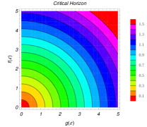
(b) $k=1$ and $q_{M}=q_{E}=0.1$.

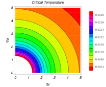
(c) $k=1$ and $g(\varepsilon)=f(\varepsilon)=1.1$.

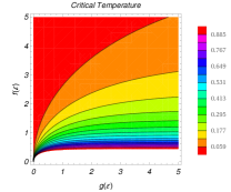
(d) $k=1$ and $q_{M}=q_{E}=0.1$.

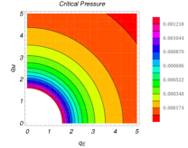
(e) $k=1$ and $g(\varepsilon)=f(\varepsilon)=1.1$.

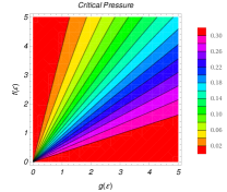
(f) $k=1$ and $q_{M}=q_{E}=0.1$.

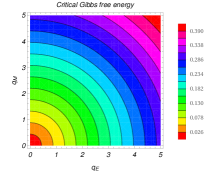
(g) $k=1$ and $g(\varepsilon)=f(\varepsilon)=1.1$.

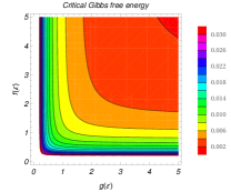
(h) $k=1$ and $q_{M}=q_{E}=0.1$.

Figure 9: Variation of the critical values as functions of black hole’s parameters.

The critical horizon radius and Gibbs free energy are increasing functions of the electric and magnetic charges while critical temperature and pressure are decreasing functions of them. As for the rainbow functions, the dependence of critical values on them is different from each case. The critical horizon radius is an increasing function of the both energy functions, whereas the critical Gibbs free energy is a decreasing function of both of them. Therefore, for these two critical values, the effects of the rainbow functions are similar. Interestingly, at the critical temperature and pressure, the effects of rainbow functions become opposite to each other. While the critical temperature and pressure are increasing functions of $g(\varepsilon)$, they are decreasing functions of $f(\varepsilon)$. The rate at which rainbow function are affecting critical horizon radius and Gibbs free energy is similar. Whereas, such rate in critical temperature and pressure is significantly different. This shows that critical behavior of temperature and pressure are significantly differently affected by one rainbow function compared to the other one. Using the critical points, we plot the following diagrams to understand the type of critical behavior (Fig. 10).

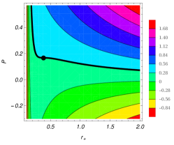
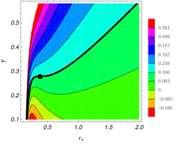
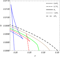
Figure 10: Van der Waals like phase diagrams for $q_{M}=q_{E}=0.1$, $f(\varepsilon)=g(\varepsilon)=1.1$ and $k=1$. The dot is the phase transition point. Left Panel: Bold line corresponds to $T=T_{c}$. Middle Panel: Bold line corresponds to $P=P_{c}$. Right Panel: Continuous line corresponds to $P=P_{c}$.

For pressures smaller than the critical pressure, swallow tail and subcritical isobars are formed in $G-T$ and $T-r_{+}$ diagrams. On the other hand, for temperatures smaller than the critical temperature, there are three different horizon radii (volumes) on the same isothermal diagrams for the same pressure in $P-r_{+}$ diagram. The behaviors observed in the mentioned diagrams point out that critical behavior of the black holes is similar to the one observed for van der Waals of the liquid-gas system. This indicates that the phase transition is first order. It could also be checked that the first order derivation of Gibbs free energy with respect to thermodynamical volume is finite at critical point. In conclusion, we find that the phase transition that we observe for these black holes is first order and the thermodynamical behavior of black holes around the critical point is van der Waals like.

IV Conclusion

In this paper, we investigated the properties of dyonic black holes in the presence of gravity’s rainbow. It was shown that due to the specific coupling of the rainbow functions with temporal and other coordinates, one is able to track the effects of different coordinates on the properties of the system including thermodynamical quantities and behavior.

We found that existence of the black hole solutions was bounded by an upper limit over rainbow functions and magnetic charge, whereas it was limited from below by the geometrical mass. Through our investigation of thermodynamical quantities, it was confirmed that rainbow functions have opposite effects (contrary to their effects on metric function). Such behavior was found to be rooted in the special coupling of these functions with temporal and spatial coordinates. In fact, this coupling resulted into non-trivial and novel effects on different thermodynamical quantities. For example, while the electric potential was independent of rainbow function, the magnetic potential was highly sensitive to variation of them. Subsequently, we observed that the black holes would enjoy phase transition and multiple phases in their structure. For super magnetized and pressurized cases, black holes thermodynamically would have only one stable phase. On the contrary, for small values of these parameters, the single-uniform-phase system would be modified into a critically active one with phase transitions and upper bounds imposed over its parameters. The effects of rainbow functions on such properties and behaviors were complicated. While for super high values of one of these rainbow functions, black holes would have single stable phase, in other cases, they would have critical behavior and separated stable phases. It was also found that small black holes would have negative temperature and hence, are non-physical. The type of phase transition reported for these black holes was first order and critical behavior was van der Waals like.

- (1) J. Magueijo and L. Smolin, Class. Quantum Grav. 21, 1725 (2004).
- (2) G. Amelino-Camelia, Phys. Lett. B 510, 255 (2001).
- (3) J. Magueijo and L. Smolin, Phys. Rev. Lett. 88, 190403 (2002).
- (4) J. Magueijo and L. Smolin, Phys. Rev. D 67, 044017 (2003).
- (5) G. Amelino-Camelia, L. Freidel, J. Kowalski-Glikman, L. Smolin, Phys. Rev. D 84, 084010 (2011).
- (6) J. Magueijo, Phys. Rev. Lett. 100, 231302 (2008).
- (7) G. Amelino-Camelia, M. Arzano, G. Gubitosi, and J. Magueijo, Phys. Rev. D 87, 123532 (2013).
- (8) M. Assanioussi, A. Dapor and J. Lewandowski, Phys. Lett. B 751, 302 (2015).
- (9) D. Mattingly, Living Rev. Rel. 8, 5 (2005).
- (10) I. P. Lobo, N. Loret and F. Nettel, Eur. Phys. J. C 77, 451 (2017).
- (11) N. A. Nilsson and M. P. Dabrowski, Phys. Dark Univ. 18, 115 (2017).
- (12) A. Chatrabhuti, V. Yingcharoenrat and P. Channuie, Phys. Rev. D 93, 043515 (2016).
- (13) J. D. Barrow and J. Magueijo, Phys. Rev. D 88, 103525 (2013).
- (14) R. Garattini and M. Sakellariadou, Phys. Rev. D 90, 043521 (2014).
- (15) A. Awad, A. F. Ali and B. Majumder, JCAP 10, 052 (2013).
- (16) G. Santos, G. Gubitosi and G. Amelino-Camelia, JCAP 08, 005 (2015).
- (17) S. H. Hendi, M. Momennia, B. Eslam Panah and S. Panahiyan, Phys. Dark Universe 16, 26 (2017).
- (18) A. F. Ali, Phys. Rev. D 89, 104040 (2014).
- (19) A. F. Ali, M. Faizal and M. M. Khalil, Nucl. Phys. B 894, 341 (2015).
- (20) A. F. Ali, M. Faizal and B. Majumder, Europhys. Lett. 109, 20001 (2015).
- (21) Y. Gim and W. Kim, JCAP 05, 002 (2015).
- (22) P. Galan and G. A. M. Marugan, Phys. Rev. D 70, 124003 (2004).
- (23) Y. W. Kim, S. K. Kim and Y. J. Park, [arXiv:1709.07755].
- (24) Y. Gim, H, Um and W. Kim, JCAP 02, 060 (2018).
- (25) R. Garattini and E. N. Saridakis, Eur. Phys. J. C 75, 343 (2015).
- (26) R. Garattini, [arXiv:1712.09728].
- (27) S. H. Hendi, G. H. Bordbar, B. Eslam Panah and S. Panahiyan, JCAP 09, 013 (2016).
- (28) D. Momeni, S. Upadhyay, Y. Myrzakulov and R. Myrzakulov, Astrophys. Space Sci. 362, 148 (2017).
- (29) K. Bakke and H. Mota, [arXiv:1802.08711].
- (30) H. L. Liu and G. L. Lu, [arXiv:1805.00333].
- (31) Y. Heydarzade, P. Rudra, F. Darabi, A. F. Ali, M. Faizal, Phys. Lett. B 774, 46 (2017).
- (32) M. He, P. Li, Z. Wang, J. C. Ding and J. B. Deng, Gen. Rel. Grav. 50, 22 (2018).
- (33) S. H. Hendi and M. Faizal, Phys. Rev. D 92, 044027 (2015).
- (34) S. H. Hendi, B. Eslam Panah and S. Panahiyan, Prog. Theor. Exp. Phys. 2016, 103A02 (2016).
- (35) S. H. Hendi, B. Eslam Panah and S. Panahiyan, Phys. Lett. B 769, 191 (2017).
- (36) S. H. Hendi, S. Panahiyan, S. Upadhyay, B. Eslam Panah, Phys. Rev. D 95, 084036 (2017).
- (37) V. B. Bezerra, H. R. Christiansen, M. S. Cunha and C. R. Muniz, Phys. Rev. D 96, 024018 (2017).
- (38) C. Leiva, J. Saavedra and J. Villanueva, Mod. Phys. Lett. A 24, 1443 (2009).
- (39) A. F. Ali, M. Faizal and B. Majumder, Europhys. Lett. 109, 20001 (2015).
- (40) P. Galan and G. A. M. Marugan, Phys. Rev. D 74, 044035 (2006).
- (41) Y. Ling, X. Li, H. Zhang, Mod. Phys. Lett. A 22, 2749 (2007).
- (42) S. H. Hendi, S. Panahiyan, B. Eslam Panah, M. Faizal and M. Momennia, Phys. Rev. D 94, 024028 (2016).
- (43) S. H. Hendi, S. Panahiyan, B. Eslam Panah and M. Momennia, Eur. Phys. J. C 76, 150 (2016).
- (44) Y. W. Kim, S. K. Kim and Y. J. Park, Eur. Phys. J. C 76, 557 (2016).
- (45) S. H. Hendi, S. Panahiyan, B. Eslam Panah, M. Faizal and M. Momennia, Phys. Rev. D 94, 024028 (2016).
- (46) S. Alsaleh, Int. J. Mod. Phys. A 32, 175007 (2017).
- (47) S. Alsaleh, Eur. Phys. J. Plus 132, 181 (2017).
- (48) Z. W. Feng and S. Z. Yang, Phys. Lett. B 772, 737 (2017).
- (49) S. H. Hendi, B. Eslam Panah, S. Panahiyan, M. Momenna, Eur. Phys. J. C 77, 647 (2017).
- (50) Z. W. Feng, [arXiv:1710.04496].
- (51) M. Dehghani, Phys. Lett. B 777, 351 (2018).
- (52) M. Dehghani, Phys. Lett. B 781, 553 (2018).
- (53) S. H. Hendi, H. Behnamifard and B. Bahrami-Asl, Prog. Theor. Exp. Phys. 2018, 033E03 (2018).
- (54) P. Li, M. He, J. C. Ding, X. R. Hu and J. B. Deng, [arXiv:1806.00361].
- (55) G. J. Cheng, R. R. Hsu and W. F. Lin, J. Math. Phys. 35, 4839 (1994).
- (56) D. A. Lowe and A. Strominger, Phys. Rev. Lett. 73, 1468 (1994).
- (57) H. Lu, Y. Pang and C.N. Pope, JHEP 11, 033 (2013).
- (58) S. Li, H. Lu and H. Wei, JHEP 07, 004 (2016).
- (59) M. Cardenas, O. Fuentealba and J. Matulich, JHEP 05, 001 (2016).
- (60) P. Meessen, T. Ortin and P. F. Ramirez, JHEP 10, 066 (2017).
- (61) K. A. Bronnikov, Grav. Cosmol. 23, 343 (2017).
- (62) E. A. Davydov, [arXiv:1711.04198].
- (63) M. Bravo-Gaete and M. Hassaine, Phys. Rev. D 97, 024020 (2018).
- (64) M. M. Caldarelli, O. J. C. Dias and D. Klemm, JHEP 03, 025 (2009).
- (65) S. A. Hartnoll and P. Kovtun, Phys. Rev. D 76, 066001 (2007).
- (66) T. Albash and C. V. Johnson, JHEP 09, 121 (2008).
- (67) K. Goldstein, N. Iizuka, S. Kachru, S. Prakash, S. P. Trivedi and A. Westphal, JHEP 10, 027 (2010).
- (68) C. M. Chen, Y. M. Huang, J. R. Sun, M. F. Wu and S. J. Zou, Phys. Rev. D 82, 066003 (2010).
- (69) R. G. Cai and R. Q. Yang, Phys. Rev. D 90, 081901 (2014).
- (70) S. Dutta, A. Jainyand and R. Soniz, JHEP 12, 060 (2013).
- (71) S. H. Hendi, N. Riazi and S. Panahiyan, Ann. Phys. (Berlin) 530, 1700211 (2018).
- (72) S. H. Hendi, S. Panahiyan, B. Eslam Panah, M. Faizal, and M. Momennia, Phys. Rev. D 94, 024028 (2016).
- (73) S. H. Hendi, B. Eslam Panah, S. Panahiyan and M. Momennia, Eur. Phys. J. C 77, 647 (2017).
- (74) D. Kubiznak and R. B. Mann, JHEP 07, 033 (2012).
- (75) S. W. Hawking, Commun. Math. Phys. 43, 199 (1975).
- (76) J. D. Beckenstein, Phys. Rev. D 7, 2333 (1973).
- (77) S. W. Hawking, Nature 248, 30 (1974).