Flocking and Target Interception Control for Formations of Nonholonomic Kinematic Agents

Abstract

In this work, we present solutions to the flocking and target interception problems of multiple nonholonomic unicycle-type robots using the distance-based framework. The control laws are designed at the kinematic level and are based on the rigidity properties of the graph modeling the sensing/communication interactions among the robots. An input transformation is used to facilitate the control design by converting the nonholonomic model into the single integrator-like equation. We assume only a subset of the robots know the desired, time-varying flocking velocity or the target’s motion. The resulting control schemes include distributed, variable structure observers to estimate the unknown signals. Our stability analyses prove convergence to the desired formation while tracking the flocking velocity or the target motion. The results are supported by experiments.

I Introduction

The field of decentralized control of multi-agent systems is an ongoing topic of interest to control and robotics researchers. Formation control is a type of coordinated behavior where mobile agents are required to autonomously converge to a specified spatial pattern. Many coordinated/cooperative tasks, such are element tracking, exploration, and object transportation, also require the formation to maneuver as a virtual rigid body. Such maneuvers can include translation, rotation, or the combination of both. When only the translational component is considered, the problem is often referred to as flocking. A related problem is called target interception where the agents intercept and surround a moving target with a given formation.

Formation control algorithms have been designed for different models of the agent motion. Most results are based on point-mass type models, such as the single and double integrator models. For example, see [20, 30, 48] for single integrator results and [9, 10, 45] for double integrator results. On the other hand, some results have used more sophisticated models that account for the agent kinematics/dynamics. One of two models are used in these cases: the fully-actuated (holonomic) Euler-Lagrange model, which includes robot manipulators, spacecraft, and some omnidirectional mobile robots; or the nonholonomic (underactuated) model, which accounts for velocity constraints that typically occur in the vehicle motion (e.g., differentially-driven wheeled mobile robots and air vehicles). In the nonholonomic case, models can be further subdivided into two categories: the purely kinematic model where the control inputs are at the velocity level, and the dynamic model where the inputs are at the actuator level. Examples of work based on the Euler-Lagrange model include [8, 12, 15, 31, 37]. Formation control results based on nonholonomic kinematic models can be found in [5, 34, 36, 41]. Designs for nonholonomic dynamic models appeared in [13, 18, 19, 21, 32].

Flocking and target interception controllers were introduced in [7, 6] for the single- and double-integrator models using the distance-based, rigid graph approach from [30] where the time-varying flocking velocity was available to all agents. A 2D formation maneuvering controller was proposed in [4] for the double-integrator model where the group leader, who has inertial frame information, passes the information to other agents through a directed path in the graph. A limitation of this control is that it becomes unbounded if the desired formation maneuvering velocity is zero. In [27], a leader-follower type solution modeled as a spanning tree was presented for the formation maneuvering problem based on the nonholonomic kinematics of unicycle robots. A combination of tracking errors and inter-agent coordination errors were used to quantify the control objective. A consensus scheme was presented in [23] using both the single- and double-integrator models where the desired flocking velocity is constant and known to only two leader agents. In [40], the flocking strategy involved a leader with a constant velocity command and followers who track the leader while maintaining the formation shape. The control law, which was based on the single-integrator model, consisted of the standard gradient descent formation acquisition term plus an integral term to ensure zero steady-state error with respect to the velocity command. In [44], a flocking controller was designed for agents modeled by double integrators that allows all agents to both achieve the same velocity and reach a desired formation in finite time. A similar problem was addressed in [16] but with asymptotic formation acquisition and velocity consensus. In [33], a controller was proposed using the single-integrator model that can steer the entire formation in rotation and/or translation in 3D. The rotation component was specified relative to a body-fixed frame whose origin is at the centroid of the desired formation and needs to be known. In [43], the authors study the flocking behavior of multiple vehicles with a dynamic leader with known acceleration available to all agents. A flocking controller was designed in [44] for double integrator agents that ensures finite time convergence for the flocking of desired formation with flocking velocity equal to the average of the agents’ initial velocity. Recently, [47] introduced a distance-based, flocking-type controller where the formation centroid tracks a reference trajectory using a finite-time centroid observer.

A special case of flocking, called consensus tracking, where the agents simply have to track the motion of a leader without being in formation was addressed in [11, 24, 35]. In [24], only the single-integrator agents connected to the leader had access to its position and a decentralized, linear observer was designed to estimate the leader’s time-varying velocity. However, exact tracking of the leader motion was only assured when the leader acceleration was known by all agents. In [35], Euler-Lagrange agents with parametric uncertainty were considered in the design of two consensus tracking algorithms. In the first design, the leader velocity was constant and an adaptive controller combined with a distributed, linear velocity observer were developed. The second design assumed the leader velocity is time-varying which leads to the formulation of a variable structure-type control law using one- and two-hop neighbor information. In [11], the authors studied single and double integrator agents in fixed and switching network topologies with constant and time-varying leader velocity. Distributed variable structure consensus tracking controllers were designed without velocity (resp., acceleration) measurements for the single (resp., double) integrator case.

A popular formation control approach is to use the inter-agent distances as the controlled variables. This approach is intrinsically related to rigid graph theory [1] since the concept of graph rigidity naturally ensures that the inter-agent distance constraints of the desired formation are enforced. The distance-based control framework has been mostly applied to the single and double integrator agent models. To the best of our knowledge, the only exceptions are the results in [17, 46]. In [17], the authors considered the nonholonomic kinematic model in the design of a formation acquisition controller. The work in [46] studied the circular formation control of nonholonomic kinematic agents with fixed (but distinct) cruising speeds.

In this paper, we apply the distance-based approach to the flocking and target interception of nonholonomic kinematic agents in the form of unicycle-type vehicles. In the flocking problem, we assume the desired, time-varying flocking velocity is known by only a subset of the agents. In the target interception problem, only the leader agent has the target information. We use an input transformation to convert the nonholonomic multi-agent system into a single integrator-like system that includes a multiplicative matrix dependent on the vehicle heading angle error. This transformation enables us to use the gradient descent law from [30] for formation acquisition augmented with a flocking or target interception term. The flocking term for each agent is a flocking velocity estimate generated by a distributed, variable structure observer using only neighbor information, which was inspired by the consensus algorithms in [11, 35]. The target interception term for the followers is composed of two estimates$-$one for the target velocity and one for the relative position of the target to the leader$-$which are also updated by distributed, variable structure observers. For both problems, the overall closed-loop system is composed of multiple coupled nonlinear subsystems. Thus, the stability of the proposed observer-controller system is analyzed using input-to-state stability and interconnected system theory. Our analyses show that the error dynamics are asymptotically stable at the origin for both problems, meaning that the flocking and target interception objectives are successively met. The main contribution of this paper is that it is the first to apply the distance-based framework to nonholonomic kinematic agents for the flocking and target interception problems. A preliminary version of this work appeared in [28] where the flocking velocity was assumed known to all agents.

II Background Material

An undirected graph $G$ is a pair $(V,E)$ where $V=\{1,2,...,n\}$ is the set of nodes and $E\subset V\times V$ is the set of undirected edges that connect two different nodes, i.e., if node pair $(i,j)\in E$ then so is $(j,i)$. We let $a\in\left\{1,\ldots,n(n-1)/2\right\}$ denote the total number of edges in $E$.  The set of neighbors of node $i$ is denoted by

$$\mathcal{N}_{i}(E)=\{j\in V\mid(i,j)\in E\}.$$ (1)

Let $A=[a_{ij}]\in\mathbb{R}^{n\times n}$ be the adjacency matrix defined such that $a_{ij}=1$ if $(i,j)\in E$ and $a_{ij}=0$ otherwise. Note that $a_{ij}=a_{ji}$. The Laplacian matrix $L=[l_{ij}]\in\mathbb{R}^{n\times n}$ associated with $A$ is defined such that $l_{ii}=\sum_{j=1,j\neq i}^{n}a_{ij}$ and $l_{ij}=-a_{ij}$ for $i\neq j$. Note that $L$ is symmetric positive definite, and has a simple zero eigenvalue with an associated eigenvector $1_{n}$ where $1_{n}$ is the $n\times 1$ vector of ones [14].

If $p_{i}\in\mathbb{R}^{2}$ is the coordinate of node $i$, then a framework $F$ is defined as the pair $\left(G,p\right)$ where $p=\left[p_{1},\ldots,p_{2}\right]\in\mathbb{R}^{2n}$. In the following, we assume all frameworks have generic properties, i.e., the properties hold for almost all of the framework representations. This is done to exclude certain degenerate configurations such as frameworks that lie in a hyperplane (see [22] for a detailed study of generic frameworks).

Based on an arbitrary ordering of edges, the edge function $\phi:$ $\mathbb{R}^{2n}\rightarrow\mathbb{R}^{a}$ is given by

$$\phi(p)=\left[...,\left\|p_{i}-p_{j}\right\|^{2},...\right],\text{ \ \ }(i,j)\in E$$ (2)

such that its $k$th component, $\left\|p_{i}-p_{j}\right\|^{2}$, relates to the $k$th edge of $E$ connecting the $i$th and $j$th nodes. The rigidity matrix $R:\mathbb{R}^{2n}\rightarrow\mathbb{R}^{a\times 2n}$ is given by

$$R(p)=\frac{1}{2}\frac{\partial\phi(p)}{\partial p}$$ (3)

where rank$\left[R(p)\right]\leq 2n-3$ [2]. Notice that the $k$th row of $R$ has the form

$$\left[0\text{ }...\text{ }0\text{ }\left(p_{i}-p_{j}\right)^{\top}\text{ }0\text{ }...\text{ }0\text{ }\left(p_{j}-p_{i}\right)^{\top}\text{ }0\text{ }\ldots\text{ }0\right]$$ (4)

where $\left(p_{i}-p_{j}\right)^{\top}$ is in columns $2i-1$ and $2i$, $\left(p_{j}-p_{i}\right)^{\top}$ is in columns $2j-1$ and $2j$, and all other elements are zero.

An isometry of $\mathbb{R}^{2}$ is a bijective map $\mathcal{T}:\mathbb{\ \mathbb{R}}^{2}\rightarrow\mathbb{\ \mathbb{R}}^{2}$ satisfying [25]

$$\left\|w-v\right\|=\left\|\mathcal{T}\left(w\right)-\mathcal{T}\left(v\right)\right\|,\quad\forall w,v\in\mathbb{R}^{2}.$$ (5)

This map includes rotations and translations of the vector $w-v$. Two frameworks are said to be isomorphic in $\mathbb{R}^{2}$ if they are related by an isometry. In this paper, we will represent the collection of all frameworks that are isomorphic to $F$ by Iso$\left(F\right)$. It is important to point out that (2) is invariant under isomorphic motions of the framework.

Frameworks $\left(G,p\right)$ and $\left(G,\hat{p}\right)$ are equivalent if $\phi(p)=\phi(\hat{p})$, and are congruent if $\left\|p_{i}-p_{j}\right\|=\left\|\hat{p}_{i}-\hat{p}_{j}\right\|$, $\forall i,j\in V$ [26]. The necessary and sufficient condition for a generic framework $\left(G,p\right)$ to be infinitesimally rigid is rank$\left[R\left(p\right)\right]=2n-3$ [25]. An infinitesimally rigid framework is minimally rigid if and only if $a=2n-3$ [1]. If the infinitesimally rigid frameworks $(G,p)$ and $(G,\hat{p})$ are equivalent but not congruent, then they are referred to as ambiguous [1]. The notation Amb$\left(F\right)$ will be used to represent the collection of all frameworks that are ambiguous to the infinitesimally rigid framework $F$. All frameworks in Amb$\left(F\right)$ are also assumed to be infinitesimally rigid. According to [1] and Theorem 3 of [3], this assumption holds almost everywhere.

Lemma 1

[7] For any $x\in\mathbb{R}^{2}$, $R(p)(1_{n}\otimes x)=0$ where $1_{n}$ is the $n\times 1$ vector of ones.

Theorem 1

[29] Consider the system $\dot{x}=f\left(x,u\right)$ where $x$ is the state, $u$ is the control input, and $f(x,u)$ is locally Lipschitz in $(x,u)$ in some neighborhood of $(x=0,u=0)$. Then, the system is locally input-to-state stable (ISS) if and only if the unforced system $\dot{x}=f(x,0)$ has a locally asymptotically stable equilibrium point at the origin.

Theorem 2

[29] Consider the interconnected system

$$\begin{array}[]{ll}\Sigma_{1}\text{:}&\dot{x}=f(t,x,y)\\ \Sigma_{2}\text{:}&\dot{y}=g(t,y).\end{array}$$ (6)

if subsystem $\Sigma_{1}$ with input $y$ is ISS and $y=0$ is a uniformly asymptotically stable equilibrium point of subsystem $\Sigma_{2}$, then $[x,y]=0$ is a uniformly asymptotically stable equilibrium point of the interconnected system.

For any piecewise continuous signal $x:\mathbb{R}_{\geq 0}\rightarrow\mathbb{R}^{n}$,

$$\left\|x\right\|_{\mathcal{L}_{\infty}}:=\sup\limits_{t\geq 0}\left\|x(t)\right\|.$$ (7)

If $\left\|x\right\|_{\mathcal{L}_{\infty}}<\infty$ (the signal is bounded for all time), we say that $x(t)\in\mathcal{L}_{\infty}$.

Finally, for any $x\in\mathbb{R}^{n}$, sgn$\left(x\right):=[sgn\left(x_{1}\right),\ldots,$ $sgn\left(x_{n}\right)]$ where $sgn(\cdot)$ is the standard signum function:

$$sgn\left(x_{i}\right)=\left\{\begin{array}[]{ll}1&\text{if }x_{i}>0\\ 0&\text{if }x_{i}=0\\ -1&\text{if }x_{i}<0.\end{array}\right.$$ (8)

III System Model

Consider a system of $n$ agents moving autonomously on the plane. Figure 1 depicts the $i$th agent, where the reference frame $\left\{X_{0},Y_{0}\right\}$ is an inertial frame. The body reference frame $\left\{X_{i},Y_{i}\right\}$ is attached to the $i$th vehicle with the $X_{i}$ axis aligned with its heading (longitudinal) direction, which is given by angle $\theta_{i}$ and measured counterclockwise from the $X_{0}$ axis. Point $C_{i}$ denotes the $i$th vehicle’s center of mass which is assumed to coincide with its center of rotation.

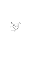
Figure 1: Schematic of the unicycle agent.

We assume the agent motion is governed by the following nonholonomic, unicycle kinematic model

$$\dot{q}_{i}=S(\theta_{i})\eta_{i},\quad i=1,...,n.$$ (9)

In (9), $q_{i}=\left[x_{i},y_{i},\theta_{i}\right]$ denotes the position and orientation of $\{X_{i},Y_{i}\}$ relative to $\{X_{0},Y_{0}\}$, $\eta_{i}=\left[v_{i},\omega_{i}\right]$ is the control input, $v_{i}$ is the $i$th agent’s translational speed in the direction of $\theta_{i}$, $\omega_{i}$ is the $i$th agent’s angular speed about the vertical axis passing through $C_{i}$, and

$$S(\theta_{i})=\begin{bmatrix}\cos\theta_{i}&0\\ \sin\theta_{i}&0\\ 0&1\end{bmatrix}.$$ (10)

IV Problem Statement

Consider that the agents’ target formation is modeled by the framework $F^{\ast}=(G^{\ast},p^{\ast})$ where $G^{\ast}=\left(V^{\ast},E^{\ast}\right)$, dim$(V^{\ast})=n$, dim$(E^{\ast})=a$, $p^{\ast}=\left[p_{1}^{\ast},\ldots,p_{n}^{\ast}\right]$, and $p_{i}^{\ast}=\left[x_{i}^{\ast},y_{i}^{\ast}\right]$. The target distance separating the $i$th and $j$th agents is given by

$$d_{ij}=\left\|p_{i}^{\ast}-p_{j}^{\ast}\right\|>0,\quad i,j\in V^{\ast}.$$ (11)

We assume $F^{\ast}$ is constructed to be infinitesimally and minimally rigid.

The actual formation of the agents is encoded by the framework $F(t)=\left(G^{\ast},p(t)\right)$ where $p=\left[p_{1},\ldots,p_{n}\right]$ and $p_{i}=\left[x_{i},y_{i}\right]$. We make the following assumptions about the agents.

1. Agent $i$ can measure the relative position of agent $j$, $p_{i}-p_{j}$, $\forall j\in\mathcal{N}_{i}(E^{\ast})$ with respect to frame $\left\{X_{i},Y_{i}\right\}$.

2. Agent $i$ can measure the relative heading angle of agent $j$, $\theta_{i}-\theta_{j}$, $\forall j\in\mathcal{N}_{i}(E^{\ast})$.

3. Agent $i$ has a communication channel with agent $j$, $\forall j\in\mathcal{N}_{i}(E^{\ast})$.

We will address the following two formation problems.

Flocking Problem: In this problem, the agents need to acquire and maintain a pre-defined geometric shape in the plane while simultaneously moving with a desired translational velocity that is known by only a subset of the agents. That is,

$$F(t)\rightarrow\text{Iso}\left(F^{\ast}\right)\text{ as }t\rightarrow\infty,$$ (12)

which is equivalent to

$$\left\|p_{i}(t)-p_{j}(t)\right\|\rightarrow d_{ij}\text{ as }t\rightarrow\infty,\quad i,j\in V^{\ast}$$ (13)

due to the framework rigidity, and

$$\dot{p}_{i}(t)-v_{0}(t)\rightarrow 0\text{ as }t\rightarrow\infty,\quad i=1,...,n$$ (14)

where $v_{0}\in\mathbb{R}^{2}$ is any continuously differentiable function of time representing the desired flocking velocity. We assume $v_{0}(t),\dot{v}_{0}(t)\in\mathcal{L}_{\infty}$ where $\left\|\dot{v}_{0}(t)\right\|_{\mathcal{L}_{\infty}}\leq\gamma_{0}$ and $\gamma_{0}$ is a known positive constant. The nonempty subset of agents that have direct access to $v_{0}$ is denoted by $V_{0}\subset V^{\ast}$.

Target Interception Problem: Here, the agents should intercept and enclose a (possibly evading) moving target with a pre-defined formation. The acquisition of the pre-defined formation is quantified by (12). Let $p_{T}\in\mathbb{R}^{2}$ denote the target position, which is assumed to be a twice continuously differentiable function of time such that $p_{T}(t),\dot{p}_{T}(t),\ddot{p}_{T}(t)\in\mathcal{L}_{\infty}$ where $\left\|\ddot{p}_{T}(t)\right\|_{\mathcal{L}_{\infty}}\leq\gamma_{T1}$ and $\gamma_{T1}\$is a known positive constant. In order to intercept the target, we use a leader-follower-like scheme where the $n$th agent is the leader and the remaining agents are followers. The leader is responsible for tracking the target while the followers flock and maintain the desired formation. Thus, the leader is the only agent that can directly measure its relative position to the target, $p_{T}-p_{n}$, and the target velocity, $\dot{p}_{T}$. The desired formation $F^{\ast}$ should be selected with the additional condition that $p_{n}^{\ast}\in$ conv$\left\{p_{1}^{\ast},...,p_{n-1}^{\ast}\right\}$ where conv$\left\{\cdot\right\}$ denotes the convex hull. The main objective for this problem is that $p_{T}(t)$ approach conv$\left\{p_{1}(t),...,p_{n-1}(t)\right\}$ as time evolves, i.e.,

$$p_{T}(t)\in\text{conv}\{p_{1}(t),\text{ }\ldots,\text{ }p_{n-1}(t)\}\text{ as }t\rightarrow\infty.$$ (15)

V Flocking Control

We begin by introducing several error variables. The relative position of agents $i$ and $j$ is defined as

$${p}_{ij}=p_{i}-p_{j}$$ (16)

while the corresponding distance error is captured by the variable [30]

$$z_{ij}=\left\|{p}_{ij}\right\|^{2}-d_{ij}^{2}.$$ (17)

The vector of all $z_{ij}$ for which $\left(i,j\right)\in E^{\ast}$ is defined as $z=\left[...,z_{ij},...\right]\in\mathbb{R}^{a}$, which is ordered as (2). Given that $\left\|{p}_{ij}\right\|\geq 0$, note that $z_{ij}=0$ if and only if $\left\|{p}_{ij}\right\|=d_{ij}$. This means that when $z=0$, the frameworks $F$ and $F^{\ast}$ are equivalent and therefore, $F=$ Iso$\left(F^{\ast}\right)$ or $F=$ Amb$\left(F^{\ast}\right)$. Next, let

$$\tilde{\theta}_{i}=\theta_{i}-\theta_{id}$$ (18)

where $\theta_{id}$ denotes the desired heading direction, which is to be specified later. Finally, since the flocking velocity $v_{0}$ is not known by all agents, $\hat{v}_{fi}\in\mathbb{R}^{2}$ will denote the flocking velocity estimate for agent $i$ and

$$\tilde{v}_{fi}=\hat{v}_{fi}-v_{0}$$ (19)

is the corresponding flocking velocity estimation error.

Before presenting the flocking control scheme, we state a useful lemma.

Lemma 2

[7] Consider the system

$$\dot{z}=-\alpha R(p)R^{\intercal}(p)z,$$ (20)

where $\alpha$ is a positive constant and $R(p)$, which was defined in (3), has full row rank. Given the sets

$$\begin{array}[]{l}\Omega_{1}=\left\{z:\Lambda(F,F^{\ast})\leq\delta\right\}\\ \\ \Omega_{2}=\left\{z:\text{dist}(p,\text{Iso}(F))<\text{dist}(p,\text{Amb}(F^{\ast}))\right\}\end{array}$$ (21)

where $\delta$ is a sufficiently small positive constant and dist$(\cdot)$ denotes the “distance” between a point and a set, if $z(0)\in\Omega_{1}$, then $z=0$ is an exponentially stable equilibrium point of (20). If in addition $z(0)\in\Omega_{1}\cap\Omega_{2}$, then $F(t)\rightarrow$ Iso$\left(F^{\ast}\right)$ as $t\rightarrow\infty$.

The main result of this section is given by the following theorem.

Theorem 3

Let $F^{\ast}$ be infinitesimally and minimally rigid, and the initial conditions for the distance errors satisfy $z(0)\in\Omega_{1}\cap\Omega_{2}$. Then, the control law

$$v_{i} = \left\|u_{i}\right\|\cos\tilde{\theta}_{i}$$ (22)

$$\omega_{i} = -c_{i}\tilde{\theta}_{i}+\dot{\theta}_{id}$$ (23)

$$u_{i} = \left[\begin{array}[]{c}u_{ix}\\ u_{iy}\end{array}\right]=-k_{a}\sum\limits_{j\in\mathcal{N}_{i}(E^{\ast})}\tilde{p}_{ij}z_{ij}+\hat{v}_{fi}$$ (26)

$$\theta_{id} = \left\{\begin{array}[]{ll}\text{atan2}(u_{iy},u_{ix}),&\text{if }u_{i}\neq 0\\ 0,&\text{if }u_{i}=0,\end{array}\right.$$ (29)

$$\overset{\cdot}{\hat{v}}_{fi}=-\alpha\text{sgn}\left(\sum_{j\in\mathcal{N}_{i}(E^{\ast})}(\hat{v}_{fi}-\hat{v}_{fj})\text{ }-b_{i}(\hat{v}_{fi}-v_{0})\right)$$ (30)

where $c_{i},k_{a}>0$ are control gains,

$$b_{i}=\left\{\begin{array}[]{ll}1,&\text{if }i\in V_{0}\\ 0,&\text{otherwise,}\end{array}\right.$$ (31)

and $\alpha>\gamma_{0}$ is the observer gain, ensures $(z,\tilde{v}_{fi},\tilde{\theta}_{i})=0$ for all $i\in V^{\ast}$ is uniformly asymptotically stable and that (12) and (14) hold.

Proof:

We first decompose (9) as follows

$$\dot{p}_{i} = \left[\begin{array}[]{c}v_{i}\cos\theta_{i}\\ v_{i}\sin\theta_{i}\end{array}\right]$$ (34)

$$\dot{\theta}_{i} = \omega_{i}.$$ (35)

Based on (29), we can express $u_{i}$ in polar form:

$$u_{ix}=\left\|u_{i}\right\|\cos\theta_{id}\quad\text{and}\quad u_{iy}=\left\|u_{i}\right\|\sin\theta_{id}.$$ (36)

Substituting (22) and (36) into (34) yields

$$\dot{p}_{i}=\left[\begin{array}[]{c}\left\|u_{i}\right\|{{\cos\tilde{\theta}_{i}\cos(\tilde{\theta}_{i}+\theta_{id})}}\\ \left\|u_{i}\right\|\cos\tilde{\theta}_{i}\sin(\tilde{\theta}_{i}+\theta_{id})\end{array}\right]$$ (37)

where (18) was used. After using (36) in ( 37), we obtain

$$\dot{p}_{i}=B(\tilde{\theta}_{i})u_{i}.$$ (38)

where

$$B(\tilde{\theta}_{i})=\left[\begin{array}[]{cc}\cos^{2}\tilde{\theta}_{i}&-\frac{1}{2}\sin 2\tilde{\theta}_{i}\\ \frac{1}{2}\sin 2\tilde{\theta}_{i}&\cos^{2}\tilde{\theta}_{i}\end{array}\right].$$ (39)

Now, taking the time derivative of (17) gives

$$\dot{z}_{ij}=\frac{d}{dt}\left({p}_{ij}^{\intercal}{p}_{ij}\right)=2{p}_{ij}^{\intercal}\left[B(\tilde{\theta}_{i})u_{i}-B(\tilde{\theta}_{j})u_{j}\right],$$ (40)

which can be rewritten in the following vector form

$$\dot{z}=2R(p)\mathbf{B}(\tilde{\theta})u$$ (41)

where (3) was used, $\mathbf{B}(\tilde{\theta})=$ diag$\left(B(\tilde{\theta}_{1}),...,B(\tilde{\theta}_{n})\right)\in\mathbb{R}^{2n\times 2n}$, $\tilde{\theta}=\left[\tilde{\theta}_{1},\ldots,\tilde{\theta}_{n}\right]\in\mathbb{R}^{n}$, and $u=\left[u_{1},\ldots,u_{n}\right]\in\mathbb{R}^{2n}$. Likewise, (26) can be rewritten as

$$u=-k_{a}R^{\intercal}(p)z+\hat{v}_{f}$$ (42)

where $\hat{v}_{f}=[\hat{v}_{f1},...,\hat{v}_{fn}]$ $\in\mathbb{R}^{2n}$. If $\tilde{v}_{f}=[\tilde{v}_{f1},...,\tilde{v}_{fn}]$ $\in\mathbb{R}^{2n}$, then from (19), we have

$$\tilde{v}_{f}=\hat{v}_{f}-1_{n}\otimes v_{0}.$$ (43)

After substituting (42) into (41), we get the closed-loop system

$$\dot{z}=-2k_{a}R\mathbf{B}(\tilde{\theta})R^{\intercal}z+2R\mathbf{B}(\tilde{\theta})(\tilde{v}_{f}+1_{n}\otimes v_{0})$$ (44)

where (43) was used.

Now, we turn our attention to the flocking velocity estimator. As part of this proof, we will show that (30) guarantees $\tilde{v}_{f}(t)\rightarrow 0$ as $t\rightarrow\infty$. First, notice that

$$\sum_{j\in N_{i}(E^{\ast})}(\hat{v}_{fi}-\hat{v}_{fj})=\sum_{j=1}^{n}a_{ij}(\hat{v}_{fi}-\hat{v}_{fj}),$$

where $a_{ij}$ are the elements of the adjacency matrix $A$. Taking the time derivative of (43) and substituting (30) gives

$$\overset{\cdot}{\tilde{v}}_{f} = -\alpha\text{sgn}\left((L\otimes I_{2})\tilde{v}_{f}+(\mathcal{B}\otimes I_{2})\tilde{v}_{f}\right)-1_{n}\otimes\dot{v}_{0}$$ (45)

$$= -\alpha\text{sgn}\left((\mathcal{M}\otimes I_{2})\tilde{v}_{f}\right)-1_{n}\otimes\dot{v}_{0}$$

where we used the fact that $\hat{v}_{fi}-\hat{v}_{fj}=\tilde{v}_{fi}-\tilde{v}_{fj}$, $\mathcal{B}:=$ diag$(b_{1},...,b_{n})$, $L$ is the Laplacian matrix, and $\mathcal{M}:=L+\mathcal{B}$. Since the graph of a rigid framework is always connected, we know that $G^{\ast}$ is connected. Therefore, we know from Lemma 3 of [24] that $\mathcal{M}$ is positive definite. Since (45) has a discontinuous right-hand side, its solution needs to be studied using nonsmooth analysis. Given that $sgn(\cdot)$ is Lebesgue measurable and essentially locally bounded, one can show the existence of generalized solutions by embedding the differential equation into the differential inclusion [42]

$$\overset{\cdot}{\tilde{v}}_{f}\in K\left[f\right](\tilde{v}_{f},t)$$ (46)

where $K\left[\cdot\right]$ is a nonempty, compact, convex, upper semicontinuous set-valued map and $f(\tilde{v}_{f},t)=-\alpha$sgn$\left(\left(M\otimes I_{2}\right)\tilde{v}_{f}\right)-\mathbf{1}_{n}\otimes\dot{v}_{0}$.

Consider the Lyapunov function candidate

$$W=\frac{1}{2}\tilde{v}_{f}^{\intercal}(M\otimes I_{2})\tilde{v}_{f}.$$ (47)

Differentiating $W$ along (46) yields [42]

$$\begin{array}[]{ll}\dot{W}&\overset{a.e.}{\in}\dfrac{\partial W_{f}}{\partial\tilde{v}}K\left[f\right](\tilde{v}_{f},t)\\ &\subset\tilde{v}_{f}^{\top}\left(\mathcal{M}\otimes I_{2}\right)\left[-\alpha\text{sgn}\left(\left(\mathcal{M}\otimes I_{2}\right)\tilde{v}_{f}\right)-\mathbf{1}_{n}\otimes\dot{v}_{0}\right]\end{array}$$ (48)

where a.e. means “almost everywhere”. If we define SGN$\left(x\right):=\left[SGN\left(x_{1}\right),\ldots,SGN\left(x_{n}\right)\right]$, $\forall x\in\mathbb{R}^{n}$ where

$$SGN\left(x_{i}\right)=\left\{\begin{array}[]{ll}1&\text{for }x_{i}>0\\ \left[-1,1\right]&\text{for }x_{i}=0\\ -1&\text{for }x_{i}<0,\end{array}\right.$$ (49)

then (48) becomes [42]

$$\dot{W} =-\alpha\tilde{v}_{f}^{\top}\left(\mathcal{M}\otimes I_{2}\right)\text{SGN }\left(\left(\mathcal{M}\otimes I_{2}\right)\tilde{v}_{f}\right)$$

$$-\tilde{v}_{f}^{\top}\left(\mathcal{M}\otimes I_{2}\right)\left(\mathbf{1}_{n}\otimes\dot{v}_{0}\right)$$

$$=-\alpha\left\|\left(\mathcal{M}\otimes I_{2}\right)\tilde{v}_{f}\right\|_{1}-\left(\mathbf{1}_{n}\otimes\dot{v}_{0}\right)^{\top}\left(\mathcal{M}\otimes I_{2}\right)\tilde{v}_{f}$$

$$=-\alpha\left\|\left(\mathcal{M}\otimes I_{2}\right)\tilde{v}_{f}\right\|_{1}-\dot{v}_{0}^{\top}\sum_{i=1}^{2n}\left[\left(\mathcal{M}\otimes I_{2}\right)\tilde{v}_{f}\right]_{i}$$

$$\leq-\alpha\left\|\left(\mathcal{M}\otimes I_{2}\right)\tilde{v}_{f}\right\|_{1}+\left\|\dot{v}_{0}\right\|_{\mathcal{L}_{\infty}}\left\|\left(\mathcal{M}\otimes I_{2}\right)\tilde{v}_{f}\right\|_{1}$$

$$\leq-\left(\alpha-\gamma_{0}\right)\left\|\left(\mathcal{M}\otimes I_{2}\right)\tilde{v}_{f}\right\|_{1}$$ (50)

where $\left\|\cdot\right\|_{1}$ is the vector 1-norm. For $\alpha>\gamma_{0}$, $\dot{W}$ is negative definite and therefore $\tilde{v}_{f}=0$ is uniformly asymptotically stable [42].

Next, after taking the derivative of (18) and substituting (35) and (23), we obtain

$$\overset{\cdot}{\tilde{\theta}}_{i}=-c_{i}\tilde{\theta}_{i},$$ (51)

which indicates that $\tilde{\theta}_{i}=0$, $\forall i\in V^{\ast}$ is exponentially stable.

Our overall closed-loop system is composed of three interconnected subsystems—(44), (45), and (51)—which are in the form of (6) with $y=[\tilde{v}_{f},\tilde{\theta}]$. First, notice that (44) with $\tilde{v}_{f}=\tilde{\theta}=0$ is the same as (20) upon application of Lemma 1. As a result, $z=0$ is exponentially stable for $z(0)\in\Omega_{1}$ by Lemma 2 and therefore, (44) is ISS with respect to $[\tilde{v}_{f},\tilde{\theta}]$ by Theorem 1. We can now invoke Theorem 2 to claim that $[z,\tilde{v}_{f},\tilde{\theta}]=0$ is a uniformly asymptotically stable equilibrium point of the interconnected system. If we choose $z(0)\in\Omega_{1}\cap\Omega_{2}$, then we know $F(t)\rightarrow$  Iso$\left(F^{\ast}\right)$ as $t\rightarrow\infty$ from Lemma 2.

Finally, since $z(t)$ is bounded, we know from (17) that $\tilde{p}_{ij}$, $\left(i,j\right)\in E^{\ast}$ is bounded. Therefore, since $z(t)\rightarrow 0$ as $t\rightarrow\infty$, we know from (26) and ( 38) that $\dot{p}_{i}(t)-v_{0}(t)\rightarrow 0$ as $t\rightarrow\infty$ for $\forall i\in V^{\ast}$. ∎

Remark 1

Since atan2$\left(0,0\right)$ is not defined, we used the definition in (29) for the desired heading angle to account for the case when $u_{i}=0$. Note that the form of the control inputs (22) and (23) is the same irrespective of $u_{i}$. When $u_{i}=0$, (51) still holds while $\dot{p}_{i}=0$ from (38), indicating that the motion of the agents remains bounded.

Remark 2

The time derivative of (29), which is needed in (23), is given by

$$\dot{\theta}_{id}=\left\{\begin{array}[]{ll}\dfrac{u_{i}^{\top}H\dot{u}_{i}}{\left\|u_{i}\right\|^{2}},&\text{if }u_{i}\neq 0\\ 0,&\text{if }u_{i}=0\end{array}\right.$$ (52)

where

$$H=\left[\begin{array}[]{cc}0&1\\ -1&0\end{array}\right],$$

$$\dot{u}_{i} = -k_{a}\sum\limits_{j\in\mathcal{N}_{i}(E^{\ast})}\left(z_{ij}I_{2}+2{p}_{ij}{p}_{ij}^{\intercal}\right)\left[B(\tilde{\theta}_{i})u_{i}-B(\tilde{\theta}_{j})u_{j}\right]$$ (53)

$$+\overset{\cdot}{\hat{v}}_{fi},$$

and (38) and (40) were used.

Remark 3

The flocking control law (22)-(29) is implementable in each agent’s local coordinate frame. To see this, let ${}^{j}\mathcal{R}_{i}\in SO(2)$ be the rotation matrix representing the orientation of $\left\{X_{i},Y_{i}\right\}$ with respect to $\left\{X_{j},Y_{j}\right\}$, and let a left superscript denote the coordinate frame in which a variable is expressed. First, since $\tilde{\theta}_{i}$ is measured from the $X_{i}$ axis, then (18) can be calculated with respect to $\left\{X_{i},Y_{i}\right\}$. In fact, the calculation of (18) does not need $\theta_{i}$ since ${}^{0}\tilde{\theta}_{i}=$ ${}^{i}\tilde{\theta}_{i}=-^{i}\theta_{id}$ where the calculation of ${}^{i}\theta_{id}$ from (29) uses ${}^{i}u_{i}$. Due to assumptions A2 and A3, ${}^{j}\mathcal{R}_{i}$ is known to agent $i$ for all $j\in\mathcal{N}_{i}(E^{\ast})$ so (30) can be calculated with respect to $\left\{X_{i},Y_{i}\right\}$. The variable $\dot{u}_{i}$ in (53) is frame invariant (i.e., it has the same form irrespective of the coordinate frame) since ${}^{0}\mathcal{R}_{i}^{\intercal}B(\tilde{\theta}_{i})\,\,^{0}\mathcal{R}_{i}=B(\tilde{\theta}_{i})$. Moreover, the term $B(\tilde{\theta}_{i})u_{i}-B(\tilde{\theta}_{j})u_{j}$ can be computed in $\left\{X_{i},Y_{i}\right\}$ with knowledge of ${}^{j}\mathcal{R}_{i}$. Likewise, $\dot{\theta}_{id}$ in (52) is frame invariant since ${}^{0}\mathcal{R}_{i}^{\intercal}H\,\,^{0}\mathcal{R}_{i}=H$. The first term of (26) is the standard formation shape control term which is known to be frame invariant [30]. Since the second term in (26) is the integral of (30), then $u_{i}$ can be calculated with respect to $\left\{X_{i},Y_{i}\right\}$. Finally, (29) can be implemented in $\left\{X_{i},Y_{i}\right\}$ once $u_{i}$ is specified relative to $\left\{X_{i},Y_{i}\right\}$.

VI Target Interception Control

Let $v_{T}:=\dot{p}_{T}$ and $e_{T}=p_{T}-p_{n}$ be the target interception error. Since these quantities are unknown to the followers, observers will be constructed to estimate them. Thus, $\hat{v}_{Ti}$ will denote the target velocity estimate for agent $i$ and

$$\tilde{v}_{Ti}=\hat{v}_{Ti}-v_{T}$$ (54)

is the target velocity estimation error. Further, $\hat{e}_{Ti}$ is the estimate of the target interception error for agent $i$ and

$$\tilde{e}_{Ti}=\hat{e}_{Ti}-e_{T}$$ (55)

is the corresponding estimation error.

Theorem 4

For initial conditions $z(0)\in\Omega_{1}\cap\Omega_{2}$, the control law composed of (22), (23), (29),

$$u_{i}=\left\{\begin{array}[]{l}-k_{a}\sum\limits_{j\in\mathcal{N}_{i}(E^{\ast})}p_{ij}z_{ij}+k_{T}\hat{e}_{Ti}+\hat{v}_{Ti},\\ \quad\text{if }i=1,...,n-1\\ k_{T}e_{T}+v_{T},\text{ if }i=n\end{array}\right.$$ (56)

$$\overset{\cdot}{\hat{v}}_{Ti}=-\alpha_{1}sgn\left(\sum_{j\in\mathcal{N}_{i}(E^{\ast})}(\hat{v}_{Ti}-\hat{v}_{Tj})+b_{i}(\hat{v}_{Tn}-v_{T})\right)$$ (57)

$$\overset{\cdot}{\hat{e}}_{Ti}=-\alpha_{2}sgn\left(\sum_{j\in\mathcal{N}_{i}(E^{\ast})}(\hat{e}_{Ti}-\hat{e}_{Tj})+b_{i}(\hat{e}_{Tn}-e_{T})\right)$$ (58)

where $k_{a},k_{T}>0$ are control gains, $\alpha_{1}>\gamma_{T1}$ and $\alpha_{2}>\gamma_{T2}$ are observer gains, $\left\|\dot{e}_{T}(t)\right\|_{\mathcal{L}_{\infty}}\leq\gamma_{T2}$, $\hat{v}_{Tn}(0)=v_{T}(0)$, and

$$b_{i}=\left\{\begin{array}[]{ll}1,&\text{if }i=n\\ 0,&\text{otherwise,}\end{array}\right.$$ (59)

renders $[z,\tilde{\theta}_{i},e_{T}]=0$ for all $i\in V^{\ast}$ uniformly asymptotically stable, and ensures that (12) and (15) are satisfied.

Proof:

First, as in the proof of Theorem 3, we can show that (23) and (57) ensure $\tilde{\theta}_{i}=0$, $\forall i\in V^{\ast}$ is an exponentially stable and $\tilde{v}_{T}=0$ is uniformly asymptotically stable for $\alpha_{1}>\gamma_{T1}$ where $\tilde{v}_{T}=[\tilde{v}_{T1},...,\tilde{v}_{Tn}]$ $\in\mathbb{R}^{2n}$.

The dynamics of the target interception error is given by

$$\dot{e}_{T}=v_{T}-B(\tilde{\theta}_{n})(v_{T}+k_{T}e_{T})$$ (60)

upon use of (38) and (56) for $i=n$. Notice that (60) is ISS with respect to input $\tilde{\theta}_{n}$ since the unforced system is given by $\dot{e}_{T}=-k_{T}e_{T}$. Therefore, by Theorem 2, the interconnection of (60) and (51) has a uniformly asymptotically stable equilibrium at $[e_{T},\tilde{\theta}_{n}]=0$.

Since (58) and (57) have a similar structure, the dynamics of the target interception estimation error can be calculated as

$$\overset{\cdot}{\tilde{e}}_{T}=-\alpha_{2}\text{sgn}((\mathcal{M}\otimes I_{2})\tilde{e}_{T})-1_{n}\otimes\dot{e}_{T}$$ (61)

where (55) was used, and $\tilde{e}_{T}=[\tilde{e}_{T1},\ldots\tilde{e}_{Tn}]\in\mathbb{R}^{2n}$. Given that $e_{T}(t),\tilde{\theta}_{n}(t),v_{T}(t)\in\mathcal{L}_{\infty}$, we know from (60) that $\dot{e}_{T}(t)\in\mathcal{L}_{\infty}$. Therefore, we know a bounding constant $\gamma_{T2}$ exists such that $\left\|\dot{e}_{T}(t)\right\|_{\mathcal{L}_{\infty}}\leq\gamma_{T2}$. It then follows from (61) that $\tilde{e}_{T}=0$ is uniformly asymptotically stable when $\alpha_{2}>\gamma_{T2}$.

From the asymptotic stability of the equilibrium $\tilde{v}_{T}=0$ and the initial condition $\hat{v}_{Tn}(0)=v_{T}(0)$, we have that $\hat{v}_{Tn}(t)=v_{T}(t)$, $\forall t\geq 0$. With this in mind, we can rewrite (56) in the following stack form

$$u=-k_{a}R_{0}^{\intercal}(p)z+\tilde{v}_{T}+k_{T}\tilde{e}_{T}+1_{n}\otimes(v_{T}+k_{T}e_{T})$$ (62)

where $R_{0}(p)$ is the rigidity matrix with the last two columns (which correspond to agent $n$) replaced by zeros. Substituting (62) into (41) gives

$$\begin{split}\dot{z}&=-2k_{a}R(p)\mathbf{B}(\tilde{\theta})R_{0}^{\intercal}(p)z+2R(p)\mathbf{B}(\tilde{\theta})[\tilde{v}_{T}+\\ &\mathbf{1}_{n}\otimes v_{T}+k_{T}(\tilde{e}_{T}+1_{n}\otimes e_{T})].\end{split}$$ (63)

Now, consider the interconnection of (63), (51), (45), (60), and (61). We will check if (63) is ISS with respect to input $(\tilde{\theta},\tilde{v}_{T},e_{T},\tilde{e}_{T})$. The unforced system is given by

$$\dot{z}=-2k_{a}R(p)R_{0}^{\intercal}(p)z.$$ (64)

It is not difficult to show that $R(p)R_{0}^{\intercal}(p)=R_{0}(p)R_{0}^{\intercal}(p)$. Moreover, due to the structure of $R(p)$ , setting its last two columns to zero does not affect its rank. Therefore, $R_{0}(p)$ also has full row rank and Lemma 2 can be invoked to conclude that $z=0$ is an exponentially stable equilibrium of (64) when $z(0)\in\Omega_{1}$. It then follows from Theorem 2 that $[z,\tilde{\theta},\tilde{v}_{T},e_{T},\tilde{e}_{T}]=0$ is a uniformly asymptotically stable equilibrium for the interconnected system. If $z(0)\in\Omega_{1}\cap\Omega_{2}$, then we know from Lemma 2 that $F(t)\rightarrow$ Iso$\left(F^{\ast}\right)$  as $t\rightarrow\infty$. Due to the manner in which $F^{\ast}$ is constructed, this implies that $p_{n}(t)\in$ conv$\{p_{1}(t),$ $\ldots,$ $p_{n-1}(t)\}$ as $t\rightarrow\infty$. Since we have proven that $e_{T}(t)\rightarrow 0$ as $t\rightarrow\infty$, then (15) holds. ∎

Remark 4

The target interception control law is also implementable in each agent’s local coordinate frame. One can show this by using the same arguments outlined in Remark 3.

VII Experimental Results

The controllers from Sections V and VI were experimentally tested on the Robotarium system [39]. This is a swarm robotics testbed located at the Georgia Institute of Technology that uses the GRITSBot as the mobile robot platform [38]. The GRITSBot is a low-cost, wheeled robot equipped with wireless communication, battery, and processing boards, and has a footprint of approximately $3\times 3$ cm². The MATLAB codes used to implement the controllers are available at github.com/milad-khaledyan/flocking_target_intercep_codes.git. Due to page limitations, only the flocking control experiment is presented below. However, a video of the target interception experiment can be seen at www.youtube.com/watch?v=HscvM7OtLVQ.

The experiment for the flocking controller (22)-(29) was conducted with five robots. The desired formation $F^{\ast}$ was set to a regular pentagon, which was made infinitesimally and minimally rigid by introducing seven edges such that $E^{\ast}=\{(1,2),(1,3),(1,4),(1,5),(2,3),(3,4),(4,5)\}$. The desired distances between all robots were given by $d_{12}=$ $d_{23}=d_{34}=d_{45}=d_{15}=0.1\sqrt{2(1-\cos\frac{2\pi}{5})}$ m and $d_{13}=d_{14}=0.1\sqrt{2(1+\cos\frac{\pi}{5})}$ m. The formation was required to move as a virtual rigid body around a circle. To this end, the desired translational maneuvering velocity was chosen as $v_{0}(t)=\left[-r\omega_{0}\sin\omega_{0}t\text{ , }r\omega_{0}\cos\omega_{0}t\right]$ m/s where $r=0.15$ m is the radius for the circular trajectory and $\omega_{0}=0.3$ rad/s. Figure 2 depicts the desired formation and desired maneuver. Only robot 1 had access to $v_{0}$.

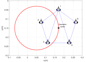
Figure 2: Desired pentagon formation along with desired circular trajectory for the geometric center.

The initial positions and orientations of the robots were randomly selected while $\hat{v}_{fi}(0)=0$ for $i=1,...,5$. The control gains in (23) and (26) were set to $c_{i}=10$, $i=1,...,5$, and $k_{a}=6$. The observer gain in (30) was set to $\alpha=0.05$ which satisfies the constraint $\alpha>\gamma_{0}$ where $\gamma_{0}=0.045=r\omega_{0}=\left\|\dot{v}_{0}(t)\right\|_{\mathcal{L}_{\infty}}$.

The path of the geometric center of the formation as it maneuvered around the circle is shown in Figure 3. This figure also shows that the desired formation was successfully acquired from the random initial configuration. Figure 4 shows the inter-agent distance errors, heading angle errors, and flocking velocity estimation errors quickly converging to approximately zero. The errors are not exactly zero due to measurement noise and the camera resolution. We can observe from the errors that the desired formation is acquired after approximately $15$ s. A video of the experiment can be seen at www.youtube.com/watch?v=nujX1QsVUJI.

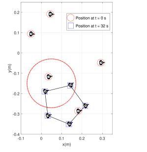
Figure 3: Circular maneuver of the geometric center of the formation along with snapshots of the formation at $t=0$ and $32$ s.

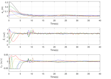
Figure 4: Distance errors, $e_{ij}(t)$, $(i,j)\in E^{\ast}$ (top), heading angle errors, $\tilde{\theta}_{i}(t)$, $i=1,...,5$ (middle), and flocking velocity estimation errors, $\tilde{v}_{fi}$, $i=1,...,5$ (bottom).

VIII Conclusion

This paper showed how the distance-based framework can be applied to nonholonomic kinematic agents to stabilize the inter-robot distances to desired values while allowing the formation to flock or track and surround a moving target. The control laws have three main components: i) an input transformation, ii) the standard gradient descent law for formation acquisition, and iii) distributed, variable structure observers to estimate the flocking or target signals not available to certain agents via their neighbors. The stability analyses showed that the proposed controls ensure the asymptotic stability of the origin of the error systems. Experimental results successfully validated the proposed formation control algorithms.

References

- [1] B.D.O. Anderson, C. Yu, B. Fidan, and J. M. Hendrickx, ”Rigid graph control architectures for autonomous formations,” IEEE Contr. Syst. Mag., vol. 28, no. 6, pp. 48-63, 2008.
- [2] L. Asimow, and B. Roth, ”The rigidity of graphs II,” J. Math. Anal. Appl., vol. 68, no. 1, pp. 171-190, 1979.
- [3] J. Aspnes, J. Egen, D.K. Goldenberg, A.S. Morse, W. Whiteley, Y.R. Yang, B.D.O. Anderson, and P.N. Belhumeur, ”A theory of network localization,” IEEE Trans. Mob. Comput., vol. 5, no. 12, pp. 1663-1678, 2006.
- [4] H. Bai, M. Arcak, and J.T. Wen, ”Using orientation agreement to achieve planar rigid formation,” Proc. Amer. Control Conf., pp. 753-758 Seattle, WA, 2008.
- [5] J. Baillieul and A. Suri, ”Information patterns and hedging Brockett’s theorem in controlling vehicle formations,” Proc. IEEE Conf. Dec. Contr., pp. 556-563, Maui, HI, 2003.
- [6] X. Cai and M. de Queiroz, ”Multi-agent formation maneuvering and target interception with double-integrator model,” Proc. Amer. Contr. Conf., pp. 287-292, Portland, OR, 2014.
- [7] X. Cai and M. de Queiroz, ”Formation maneuvering and target interception for multi-agent systems via rigid graphs,” Asian J. Contr., vol. 17, no. 4, pp. 1174-1186, 2015.
- [8] X. Cai and M. de Queiroz, ”Adaptive rigidity-based formation control for multi-robotic vehicles with dynamics,” IEEE Trans. Contr. Syst. Tech., vol. 23, no. 1, pp. 389-396, 2015.
- [9] X. Cai and M. de Queiroz, ”Rigidity-based stabilization of multi-agent formations,” ASME J. Dyn. Syst. Meas. Contr., vol. 136, no. 1, Paper 014502, 2014.
- [10] Y. Cao, D. Stuart, W. Ren, and Z. Meng, ”Distributed containment control for multiple autonomous vehicles with double-integrator dynamics: algorithms and experiments,” IEEE Trans. Contr. Syst. Tech., vol. 19, no. 4, pp. 929-938, 2011.
- [11] C. Cao and W. Ren, ”Distributed coordinated tracking with reduced interaction via a variable structure approach,” IEEE Trans. Autom. Contr., vol. 57, no. 1, pp 33-48, 2012.
- [12] G. Chen and F.L. Lewis, ”Distributed adaptive tracking control for synchronization of unknown networked lagrangian systems,” IEEE Trans. Syst. Man Cybern. - Part B, vol. 41, no. 3, pp. 805-816, 2011.
- [13] J. Chen, D. Sun, J. Yang, and H. Chen, ”Leader-follower formation control of multiple non-holonomic mobile robots incorporating a receding-horizon scheme,” Intl. J. Rob. Res., vol. 29, no. 6, pp. 727-747, 2010.
- [14] F. R. K. Chung, Spectral Graph Theory. Providence, RI: Amer. Math. Soc., 1997.
- [15] S.-J. Chung and J.-J. Slotine, ”Cooperative robot control and concurrent synchronization of Lagrangian systems,” IEEE Trans. Rob., vol. 25, no. 3, pp. 686-700, 2009.
- [16] M. Deghat, B.D.O. Anderson, and Z. Lin, ”Combined flocking and distance-based shape control of multi-agent formations,” IEEE Trans. Autom. Contr., vol. 61, no. 7, pp. 1824-1837, 2016.
- [17] D. V. Dimarogona and K. H. Johansson, ”Further results on the stability of distance-based multi-robot formations,” Proc. American Contr. Conf., pp. 2972-2977, St. Louis, MO, 2009.
- [18] W. Dong and J. A.Farrell, ”Cooperative control of multiple nonholonomic mobile agents,” IEEE Trans. Autom. Contr., vol. 53, no. 6, pp. 1434-1448, 2008.
- [19] W. Dong and J. A.Farrell, ”Decentralized cooperative control of multiple nonholonomic dynamic systems with uncertainty,” Automatica, vol. 45, no. 3, pp. 706-710, 2009.
- [20] F. Dörfler and B. Francis, ”Geometric analysis of the formation problem for autonomous robots,” IEEE Trans. Autom. Contr., vol. 55, no. 10, pp. 2379-2384, 2010.
- [21] V. Gazi, B. Fidan, R. Ordóñez, and M.I. Köksal, ”A target tracking approach for nonholonomic agents based on artificial potentials and sliding model control,” ASME J. Dyn. Syst. Measur. Contr., vol. 134, no. 11, Paper 061004, 2012.
- [22] J. Graver, B. Servatius, and H. Servatius. Combinatorial rigidity. Providence, RI: American Mathematical Society, 1993.
- [23] Z. Han, L. Wang, Z. Lin, and R. Zheng, ”Formation control with size scaling via a complex Laplacian-based approach,” IEEE Trans. Cyber., vol. 46, no. 10, pp. 2348-2359, 2016.
- [24] Y. Hong, J. Hu, and L. Gao, ”Tracking control for multi-agent consensus with an active leader and variable topology,” Automatica, vol. 42, no. 7 pp. 1177-1182, 2006.
- [25] I. Izmestiev, ”Infinitesimal rigidity of frameworks and surfaces,” Lectures on Infinitesimal Rigidity, Kyushu University, Japan, 2009.
- [26] B. Jackson, ”Notes on the rigidity of graphs,” Notes of the Levico Conference, 2007.
- [27] M. Khaledyan and M. de Queiroz, ”A formation maneuvering controller for multiple nonholonomic robotic vehicles,” Robotica, in press, DOI: 10.1017/S0263574718000942.
- [28] M. Khaledyan and M. de Queiroz, ”Translational maneuvering control of nonholonomic kinematic formations: Theory and experiments,” Proc. Amer. Control Conf., pp. 2910-2915, Milwaukee, WI, 2018.
- [29] H.K. Khalil. Nonlinear Systems. Prentice Hall, Englewood Cliffs, NJ, 2002.
- [30] L. Krick, M.E. Broucke, and B.A. Francis, ”Stabilization of infinitesimally rigid formations of multi-robot networks,” Intl. J. Contr., vol. 83, no. 3, pp. 423-439, 2009.
- [31] D. Lee and P.Y. Li, ”Passive decomposition approach to formation and maneuver control of multiple rigid-bodies,” ASME J. Dyn. Syst. Measur. Contr., vol. 129, no. 5, pp. 662-677, 2007.
- [32] Y. Liang and H.-H. Lee, ”Decentralized formation control and obstacle avoidance for multiple robots with nonholonomic constraints,” Proc. Amer. Contr. Conf., pp. 5596-5601, Minneapolis, MN, 2006.
- [33] H.G. de Marina, B. Jayawardhana, and M. Cao, ”Distributed rotational and translational maneuvering of rigid formations and their applications,” IEEE Trans. Rob., vol. 32, no. 3, pp. 684-697, 2016.
- [34] S. Mastellone, D.M. Stipanovic, C.R.Graunke, K.A. Intlekofer, and M.W. Spong, ”Formation control and collision avoidance for multi-agent non-holonomic systems: theory and experiments,” Intl. J. Robotics Res., vol. 27, no. 1, pp. 107-126, 2008.
- [35] J. Mei, W. Ren, and G. Ma, ”Distributed coordinated tracking with a dynamic leader for multiple Euler-Lagrange systems,” IEEE Trans. Autom. Contr., vol. 56, no. 6, pp. 1415-1421, 2011.
- [36] N. Moshtagh, N. Michael, A. Jadbabaie, and K. Daniilidis, ”Vision-based, distributed control laws for motion coordination of nonholonomic robots,” IEEE Trans. Rob., vol. 25, no. 4, pp. 851-860, 2009.
- [37] A.R. Pereira, L. Hsu, and R. Ortega, ”Globally stable adaptive formation control of Euler-Lagrange agents via potential functions,” Proc. Amer. Contr. Conf., pp. 2606-2611, St. Louis, MO, 2009.
- [38] D. Pickem, L. Wang, P. Glotfelter, Y. Diaz-Mercado, M. Mote, A. Ames, E. Feron, and M. Egerstedt, ”Safe, remote-access swarm robotics research on the robotarium. arXiv preprint arXiv:1604.00640,” 2016.
- [39] D. Pickem, P. Glotfelter, L. Wang, ”The robotarium: a remotely accessible swarm robotics research testbed. arXiv preprint arXiv:1609.04730,” 2016.
- [40] O. Rozenheck, S. Zhao, and D. Zelazo, ”A proportional-integral controller for distance based formation tracking,” Proc. Europ. Contr. Conf., pp. 1693-1698, Linz, Austria, 2015.
- [41] A. Sadowska, D. Kostić, N. van de Wouw, H. Huijberts, and H. Nijmeijer, ”Distributed formation control of unicycle robots,” IEEE Conf. Rob. Autom., pp. 1564-1569, Saint Paul, MN, 2012.
- [42] D. Shevitz and B. Paden, ”Lyapunov stability of nonsmooth systems,” IEEE Trans. Autom. Contr., vol. 39, no. 9, pp. 1910-1914, 1994.
- [43] H. Shi, L. Wang, and T. Chu, ”Flocking of multi-agent systems with a dynamic virtual leader,” Intl. J. Control, vol. 82, no. 1, pp. 43-58, 2009.
- [44] Z. Sun, S. Mou, M. Deghat, and B.D.O. Anderson, ”Finite time distributed distance-constrained shape stabilization and flocking control for d-dimensional undirected rigid formations,” Intl. J. Rob. Nonl. Contr., vol. 26, pp. 2824-2844, 2016.
- [45] Z. Sun, B.D.O. Anderson, M. Deghat, and H.-S. Ahn, ”Rigid formation control of double-integrator systems,” Intl. J. Contr., vol. 90, no. 7, pp. 1403-1419, 2017.
- [46] Z. Sun, H.G. de Marina, G.S. Seyboth, B.D.O. Anderson, and C. Yu, ”Circular formation control of multiple unicycle-type agents with nonidentical constant speeds,” IEEE Trans. Contr. Syst. Tech., in press, DOI: 10.1109/TCST.2017.2763938.
- [47] Q. Yang, M. Cao, H.G. de Marina, H. Fang, and J. Chen, ”Distributed formation tracking using local coordinate systems,” Syst. & Contr. Lett., vol. 111, pp. 70-78, 2018.
- [48] P. Zhang, M. de Queiroz, and X. Cai, ”3D dynamic formation control of multi-agent systems using rigid graphs,” ASME J. Dyn. Syst. Measur. Contr., vol. 137, no. 11, Paper 111006, 2015.