Effective-one-body multipolar waveform for
tidally interacting binary neutron stars up to merger

Abstract

Gravitational-wave astronomy with coalescing binary neutron star sources requires the availability of gravitational waveforms with tidal effects accurate up to merger. This article presents an improved version of TEOBResum, a nonspinning effective-one-body (EOB) waveform model with enhanced analytical information in its tidal sector. The tidal potential governing the conservative dynamics employs resummed expressions based on post-Newtonian (PN) and gravitational self-force (GSF) information. In particular, we compute a GSF-resummed expression for the leading-order octupolar gravitoelectric term and incorporate the leading-order gravitomagnetic term (either in PN-expanded or GSF-resummed form). The multipolar waveform and fluxes are augmented with gravitoelectric and magnetic terms recently obtained in PN. The new analytical information enhances tidal effects toward merger accelerating the coalescence. We quantify the impact on the gravitational-wave phasing of each physical effect. The most important contribution is given by the resummed gravitoelectric octupolar term entering the EOB interaction potential, that can yield up to 1 rad of dephasing (depending on the NS model) with respect to its nonresummed version. The model’s energetics and the gravitational wave phasing are validated with eccentricity-reduced and multi-resolution numerical relativity simulations with different equations of state and mass ratios. We also present EOB-NR waveform comparisons for higher multipolar modes beyond the dominant quadrupole one.

I Introduction

The analysis of gravitational waves (GW) from binary neutron star events requires detailed waveform models that include tidal effects Abbott et al. (2017, 2018a, 2018b). Semi-analytical inspiral waveforms with tidal effects valid up to merger have been constructed to date only in a few works Baiotti et al. (2010); Bernuzzi et al. (2012a, 2015); Hinderer et al. (2016). These models build on the effective-one-body (EOB) formalism for the general-relativistic two-body problem Buonanno and Damour (1999, 2000) and its extension to include tidal interactions Damour and Nagar (2010). Their common starting point is the general-relativistic theory of tidal properties of neutron stars (NSs) Damour (1983); Hinderer (2008); Flanagan and Hinderer (2008); Damour and Nagar (2009a); Binnington and Poisson (2009) and a post-Newtonian (PN) expression for the EOB potential based on the calculations of Refs. Hinderer et al. (2010); Damour and Nagar (2010); Vines and Flanagan (2010); Vines et al. (2011); Damour et al. (2012a); Bini et al. (2012); Bini and Damour (2014). The conservative part of the dynamics of circularized binaries is currently known at next-to-next-to-leading order (NNLO), i.e., formal 7PN level Bini et al. (2012) (or 2PN, since the Newtonian contribution starts in fact at 5PN Damour (1983)). On the other hand, for generic, noncircular motion, the conservative dynamics is fully known only at 6PN Vines and Flanagan (2010), since Ref. Bini et al. (2012) only focused on circular motion. In addition, the tidal correction to the waveform amplitude is analytically known at 6PN Vines and Flanagan (2010), including gravitomagnetic and subdominant gravitoelectric multipolar contributions Banihashemi and Vines (2018). Note that waveform amplitude corrections due to tidal-tail terms are also exactly known analytically up to relative 2.5PN (i.e., global 7.5PN order ) thanks to the analytical knowledge of the resummed tail factor that enters the factorized EOB waveform Damour et al. (2009); Faye et al. (2015).

Such a large amount of analytical information has been compared over time with numerical relativity (NR) simulations of inspiralling and coalescing neutron stars of increased accuracy Damour and Nagar (2010); Baiotti et al. (2010); Bernuzzi et al. (2012a); Hotokezaka et al. (2013). It was pointed out as early as in Ref. Damour and Nagar (2010) that the EOB treatment of tidal effects (at the time just at 1PN level) seemed prone to underestimating their actual magnitude in the last few inspiral orbits up to merger. This fact became progressively apparent as the reliability of NR simulations increased, with improved handling of the error budget Bernuzzi et al. (2012b, a); Hotokezaka et al. (2013); Bernuzzi et al. (2015), clearly pointing out that the gravitational attraction yielded by the EOB interaction potential based on PN-expanded NNLO tidal information was not sufficiently strong so as to match the NR predictions within their error bars. Bini and Damour Bini and Damour (2014) proposed to blend together the aforementioned NNLO tidal information with gravitational-self-force (GSF) Dolan et al. (2015) information in a special resummed expression for the (gravitoelectric) potential which enhanced the tidal attraction due to the presence of a pole at the Schwarzschild light-ring. Such a potential was incorporated (with a modification concerning the light-ring location, see below) in the (nonspinning) TEOBResum model Bernuzzi et al. (2015), that is built upon of the point-mass, nonspinning, EOB dynamics of Refs. Damour and Nagar (2014); Nagar et al. (2017, 2018). The key prescription suggested in Ref. Bini and Damour (2014) and implemented Ref. Bernuzzi et al. (2015) is to substitute the test-mass light-ring pole $r=3$ (in dimensionless units) with the the light-ring of the NNLO EOB model. The pole effectively amplifies tides in a regime in which the two NS cannot be described as isolated objects. Note that the pole singularity is never reached since the EOB dynamics terminates at a larger radius. TEOBResum reproduces NR waveforms within their errors up to merger for a large sample of binaries, including binaries with nonprecessing spins Bernuzzi et al. (2015); Nagar et al. (2018); Dietrich and Hinderer (2017). To date, TEOBResum has been tested against the largest sample of NR data available Dietrich et al. (2018a). Some phase differences with respect to the NR data are however present for binaries with large mass ratio and/or for NS with large tidal polarizability parameters, thus indicating that reproducing the GW from last few orbits using EOB requires even stronger tides Bernuzzi et al. (2015); Dietrich and Hinderer (2017); Nagar et al. (2018); Hotokezaka et al. (2015, 2016).

A possible mechanism leading to an effective amplification of tidal effects close to merger is the resonance between the NS $f$-mode and the orbital frequency, cf., e.g., Refs. Kokkotas and Schäfer (1995); Ho and Lai (1999). This idea has been implemented in the EOB formalism in Refs. Hinderer et al. (2016); Steinhoff et al. (2016), and there it is referred to as “dynamical tides”. The point-mass EOB baseline used in those works is the one developed in Refs. Pan et al. (2011, 2014a, 2014b); Taracchini et al. (2014) in combination with the PN tidal NNLO EOB potential. When compared to NR data, the model has performances very similar to the GSF resummation approach. Notably, both methods either reproduce the data within their errors or slightly underestimate the GW phase near merger Dietrich and Hinderer (2017).

In this work we incorporate in TEOBResum all the analytical tidal information that is currently available: (i) the $\ell=3$ GSF-resummed contribution to the EOB $A$ potential, that is computed in this paper for the first time; (ii) the gravitomagnetic tidal potential; (iii) the tidal contributions to the EOB $B$ potential of Ref. Vines and Flanagan (2010), and (iv) the full 1PN tidal corrections to the multipolar waveform Banihashemi and Vines (2018). We then compare the performance of the model against long-end, error-controlled, NR data computed by the computational relativity (CoRe) collaboration.

The paper is organized as follows. In Sec. II.1, we compute a GSF-resummed expression for the electric $\ell=3$ term of the tidal EOB $A_{\text{T}}$ potential [cf. Eq. (5) ]. We also include the LO gravitomagnetic, $(2-)$, term either in PN series or in GSF-resummed form. We additionally incorporate the leading order tidal correction to the $B$ potential [cf. Eq. (30) ], as computed in Ref. Vines and Flanagan (2010). The gravitoelectric and gravitomagnetic corrections to the tidal multipolar waveform computed in Ref. Banihashemi and Vines (2018) are also incorporated into the factorized and resummed EOB waveform. In Sec. III, we evaluate the effect of each new term on the GW phasing for a set of sample binaries. We find that the largest effect on the tidal phase is generated by the new GSF-resummed $\ell=3$ electric term, with significantly smaller contributions from the gravitomagnetic term, the tidal correction to the $B$ potential and the sub-dominant multipoles. We also consider the gravitomagnetic contribution parameterized by static Love numbers Landry and Poisson (2015) (as opposed to irrotational) and find that this gravitomagnetic effect is also very small. The TEOBResum/NR comparison is driven in Sec. IV and concerns both the energetics (through the gauge-invariant relation between binding energy and orbital angular momentum) and the phasing, notably considering also higher multipolar modes. In particular, we consider twelve best eccentricity-reduced and multiple-resolution simulations of irrotational and quasi-circular binary neutron star mergers computed by the CoRe collaboration Dietrich et al. (2018a) and previously presented in Ref. Dietrich et al. (2017a). The high accuracy of these data currently provides us with the most stringent strong-field constraints available from NR, as shown in Fig. 9. Within this data set, we also consider simulation data with mass ratios other than unity such as $q\approx(1.5,1.75,2)$ computed in Refs. Dietrich et al. (2015, 2017b); Dietrich and Hinderer (2017). While these data are less accurate, they give some insights on the model performances in an “extreme” region of the parameter space. We additionally present comparisons of NR and EOB waveforms for modes beyond the leading-order quadrupole in Fig. 11. Conclusions are collected in Sec. V. The paper is then completed by two technical Appendixes. Appendix A reports the explicit derivation of the GSF-resummed $\ell=3$ tidal potential. Appendix B briefly discusses the numerical implementation of the model, focusing in particular on the performances yielded by the use of the post-adiabatic approximation of Ref. Nagar and Rettegno (2018).

We use geometric units $c=G=1$. To convert from geometric to physical units we recall that $GM_{\odot}/c^{3}=4.925490947\times 10^{-6}$ sec. The $(2,2)$-mode GW frequency, $f$, relates to the dimensionless $(2,2)$-mode angular frequency $\hat{\omega}$ via $f\approx 32.3125\,\hat{\omega}\,(M_{\odot}/M)\,$kHz Damour and Nagar (2010). For example, $\hat{\omega}\approx 8.356\times 10^{-4}$ at $f=10\,$Hz for a typical NS binary with $M=2.7M_{\odot}$. For the remainder of this article, we employ dimensionless units rescaled with respect to $M$.

II Tidal effects in TEOBResum

This section summarizes the main analytical results. We use the following definitions:

$$q\equiv\frac{m_{A}}{m_{B}}\geq 1\ ,\quad X_{A}\equiv\frac{m_{A}}{M}$$ (1)

with $A,B$ labelling the stars and $M=m_{A}+m_{B}$. Let us also introduce the symmetric mass ratio $\nu\equiv X_{A}X_{B}$.

II.1 Tidal potential: Gravitoelectric and magnetic terms

The key idea of EOB is to map the binary motion to geodesic motion in an effective Schwarzschild spacetime (or Kerr for binaries with spin). The dynamics are described by the following EOB Hamiltonian

$$H_{\text{EOB}}=M\sqrt{1+2\nu(\hat{H}_{\text{eff}}-1)},$$ (2)

which is given by

$$\hat{H}_{\text{eff}}=\sqrt{p_{r_{\ast}}^{2}+A(r)\left(1+\frac{p_{\varphi}^{2}}{r^{2}}+2\nu(4-3\nu)\frac{p_{r_{\ast}}^{4}}{r^{2}}\right)}$$ (3)

in polar coordinates $(r,\varphi)$ and per unit mass conjugate momenta $(p_{r_{\ast}},p_{\varphi})$ for planar motion Buonanno and Damour (1999, 2000); Damour (2001). It has been shown that the point-mass dynamics is well described by a Padé resummation of the 5PN expression for the radial potential $A(r)$ Damour and Nagar (2009b) (henceforth the point-mass potential $A_{0}$).

In EOB, the tidal interaction for quasicircular inspiral dynamics is incorporated by augmenting the point-mass potential as follows Damour and Nagar (2010)

$$A=A_{0}+A_{\text{T}},$$ (4)

where

$$A_{\text{T}}(u)=\sum_{l\geq 2} A^{(\ell+)\text{LO}}_{A}(u)\hat{A}^{(\ell+)}_{A}(u)$$

$$+ A^{(\ell-)\text{LO}}_{A}(u)\hat{A}^{(\ell-)}_{A}(u)+\left(A\leftrightarrow B\right)\ ,$$ (5)

where the signs $\pm$ correspond to gravitoelectric and gravitomagnetic terms, respectively, and $u=M/r$ is the inverse of the dimensionless EOB radial coordinate. The leading-order (LO) terms are given by

$$A^{(\ell+)\text{LO}}_{A}(u) =-\kappa^{(\ell+)}_{A}u^{2\ell+2},$$ (6a)

$$A^{(\ell-)\text{LO}}_{A}(u) =-\kappa^{(\ell-)}_{A}u^{2\ell+3},$$ (6b)

where

$$\kappa^{(\ell+)}_{A} =2{k_{A}^{(\ell)}}\frac{X_{B}}{X_{A}}\frac{X_{A}^{2\ell+1}}{\mathcal{C}_{A}^{2\ell+1}}$$ (7a)

For the $$(\ell-)$$ sector, we currently have

$$\kappa^{(2-)}_{A}=\frac{1}{2}{j_{A}^{(2)}}\frac{X_{B}}{X_{A}}\frac{X_{A}^{5}}{\mathcal{C}_{A}^{5}}.$$ (7b)

$k_{A}^{(\ell)}$ and $j_{A}^{(\ell)}$ are the dimensionless gravitoelectric and gravitomagnetic Love numbers Damour and Nagar (2009a), and $\mathcal{C}_{A}\equiv m_{A}/R_{A}$ is the compactness parameter. $k^{(\ell)}_{A}$ is often denoted as $k_{\ell}$ in the literature and relates to the other commonly used Love number (polarizability) $\bar{\lambda}_{\ell}$ via $k_{\ell}=(2\ell-1)!!\,\mathcal{C}^{2\ell+1}\bar{\lambda}_{\ell}/2$ Yagi (2014) which, in our notation, translates to

$$\Lambda^{(\ell)}_{A}\equiv\frac{2}{(2\ell-1)!!}\,\mathcal{C}^{-(2\ell+1)}_{A}k^{(\ell)}_{A}\ .$$ (8a)

Similarly, for the gravitomagnetic sector, we have

$$\Sigma^{(\ell)}_{A}\equiv\frac{\ell-1}{4(\ell+2)}\frac{1}{(2\ell-1)!!}\,\mathcal{C}_{A}^{-(2\ell+1)}j^{(\ell)}_{A}$$ (8b)

which is denoted by $\bar{\sigma}^{(\ell)}$, e.g., in Ref. Yagi (2014). For $\ell=2$, our gravitomagnetic Love number $j^{(2)}$ relates to the $k_{2}^{\text{mag}}$ of Ref. Landry and Poisson (2015) via $k_{2}^{\text{mag}}=j^{(2)}/(24\mathcal{C})$ Banihashemi and Vines (2018); Pani et al. (2018). We use quasi-universal fitting relations to obtain $\Sigma$ from $\Lambda$ Jimenez-Forteza et al. (2018); Yagi (2014); Yagi and Yunes (2013), specifically the fits of Ref. Jimenez-Forteza et al. (2018).

Following Ref. Damour and Nagar (2009a), we introduce their $\kappa^{T}_{2}\equiv\kappa^{(2+)}_{A}+\kappa^{(2+)}_{B}$ and, similarly, $\kappa^{T}_{2-}\equiv\kappa^{(2-)}_{A}+\kappa^{(2-)}_{B}$. For $q=1$, we use $\Lambda\equiv\Lambda^{(2)}_{A}=\Lambda^{(2)}_{B}$ and $\Sigma\equiv\Sigma^{(2)}_{A}=\Sigma^{(2)}_{B}$. These relations yield $\kappa^{T}_{2}=3\Lambda/16$ and $\kappa^{T}_{2-}=3\Sigma/2$. We will employ $\kappa^{T}_{2}$ and $\Lambda$ interchangeably to quantify the strength of the tidal interactions including gravitomagnetic cases as $|\Sigma|$ grows monotonically with $\Lambda$.

The potentials $\hat{A}_{A}^{(\ell\pm)}(u)$ contain the terms beyond LO. In particular, the $(\ell+)$ contributions are known up to $\ell=3$ as a series in $u$

$$\hat{A}^{(\ell+)}_{A}(u)=1+\alpha^{(\ell+)}_{1A}u+\alpha^{(\ell+)}_{2A}u^{2}\ .$$ (9)

with

$$\alpha^{(2+)}_{1A} =\frac{5}{2}X_{A},$$ (10)

$$\alpha^{(2+)}_{2A} =3+\frac{1}{8}X_{A}+\frac{337}{28}X_{A}^{2},$$ (11)

$$\alpha^{(3+)}_{1A} =-2+\frac{15}{2}X_{A},$$ (12)

$$\alpha^{(3+)}_{2A} =\frac{8}{3}-\frac{311}{24}X_{A}+\frac{110}{3}X_{A}^{2}.$$ (13)

For $\ell=4$, we are currently limited to the LO term, thus $\hat{A}_{A}^{(4+)}(u)=1$.

In the $(\ell-)$ sector, only the gravitomagnetic NLO term is known:

$$\alpha^{(2-)}_{1A} =1+\frac{11}{6}X_{A}+X_{A}^{2}.$$ (14)

Ref. Bini and Damour (2014) offered an alternative series representation for the tidal potentials $\hat{A}^{(\ell\pm)}_{A}(u)$ in terms of the mass ratio $X_{A}$ as a consequence of a resummation procedure done using results from first-order GSF approach. Using $X_{A}=m_{A}/M\ll 1$ as an expansion parameter, they wrote

$$\hat{A}^{(\ell\pm)}_{A}(u)=\hat{A}^{(\ell\pm)\text{0GSF}}+X_{A}\hat{A}^{(\ell\pm)\text{1GSF}}+X_{A}^{2}\hat{A}^{(\ell\pm)\text{2GSF}}+\ldots$$ (15)

For the 1GSF terms, Ref. Bini and Damour (2014) introduced light-ring (LR) singularity factorized potentials $\tilde{A}^{(2\pm)}(u)\equiv(1-3u)^{7/2}\hat{A}^{(2\pm)1\text{GSF}}$. Using Ref. Dolan et al. (2015)’s numerical GSF data, they constructed a global four-parameter fit to $\tilde{A}^{(2\pm)}(u)$ and explicitly displayed the fit parameters for the $(2+)$ potential. As Ref. Dolan et al. (2015)’s numerical data received a minor, $\sim\mathcal{O}(10^{-5})$, correction after the publication of Ref. Bini and Damour (2014), we repeated their fit to

$$\tilde{A}^{(2+)}(u)\approx\frac{5}{2}u\,(1-a_{1}u)(1-a_{2}u)\,\frac{1+n_{1}u}{1+d_{2}u^{2}}$$ (16)

and obtained the following minor changes to their fit parameters

$$a_{1} =8.53352,\quad a_{2}=3.04309,$$

$$n_{1} =0.840064,\quad d_{2}=17.7324.$$ (17)

These should be compared with Eq. (7.27) of Ref. Bini and Damour (2014).

For the $(2-)$ potential, we employ a similar fit using Ref. Dolan et al. (2015)’s updated data:

$$\tilde{A}^{(2-)}(u)\approx\frac{11}{6}u\,(1-a^{-}_{1}u)(1-a^{-}_{2}u)\,\frac{1+n_{1}^{-}u}{1+d_{2}^{-}u^{2}}$$ (18)

with

$$a_{1}^{-} =\ 0.728591,$$ (19)

$$a_{2}^{-} =3.10037,$$ (20)

$$n_{1}^{-} =-15.0442,$$ (21)

$$d_{2}^{-} =12.5523.$$ (22)

For the 0GSF, 2GSF potentials, from Ref. Bini and Damour (2014) we have

$$\hat{A}^{(2+)0\text{GSF}} =1+\frac{3u^{2}}{1-3u}$$ (23)

$$\hat{A}^{(2+)2\text{GSF}} =\frac{337}{28}\frac{u^{2}}{(1-3u)^{p}}$$ (24)

$$\hat{A}^{(2-)0\text{GSF}} =\frac{1-2u}{1-3u},$$ (25)

$$\hat{A}^{(2-)2\text{GSF}} =\frac{u}{(1-3u)^{p_{2-}}},$$ (26)

where the values of $p,p_{2-}$ are currently unknown due to lack of second-order GSF results. However, Sec. VIID of Ref. Bini and Damour (2014) provided a proof that $p,p_{2-}\geq 4$ and a further argument that $p\leq 6$.

We now wish to resum the $(3+)$ tidal potential in the same fashion as was done for the $(2\pm)$ tidal potentials. To this end, we introduce the following GSF series for $\hat{A}^{(3+)}_{A}(u)$

$$\hat{A}_{A}^{(3+)}(u)= (1-2u)\left(1+\frac{8}{3}\frac{u^{2}}{(1-3u)}\right)+X_{A}\,\frac{\tilde{A}^{(3+)}}{(1-3u)^{7/2}}$$

$$+X_{A}^{2}\,\frac{110}{3}\frac{u^{2}}{(1-3u)^{p_{3+}}},$$ (27)

where $p_{3+}\geq 4$ Bini and Damour (2014). Next, using Refs. Dolan et al. (2015); Nolan et al. (2015)’s numerical data, we construct a global fit for the LR factorized 1GSF potential:

$$\tilde{A}^{(3+)}(u) \equiv(1-3u)^{7/2}\hat{A}^{(3+)\text{1GSF}}$$ (28)

$$\approx \frac{15}{2}u(1+C_{1}u+C_{2}u^{2}+C_{3}u^{3})\,\frac{1+C_{4}u+C_{5}u^{2}}{1+C_{6}u^{2}},$$

with

$$C_{1} =-3.68210,\ C_{2}=5.17100,\ C_{3}=-7.63916,$$

$$C_{4} =-8.63278,\ C_{5}=16.3601,\ C_{6}=\ \ 12.3197\,.$$ (29)

The details of this derivation are collected in Appendix A.

To pragmatically reduce the number of unknowns here we set $p_{2-}=p_{3+}=p$ and we mostly stick to the (conservative) value $p=4$, as in Ref. Bernuzzi et al. (2015). However, to get an idea of the sensitivity of our results to the changes in $p$, we shall also show some results obtained using $p=9/2$. In principle, since the complete tidal potential is analytically known only at 2PN relative order, one may think to transform the parameters $\{p,p_{2-},p_{3+}\}$ into effective functions (that may depend on EOS and mass ratio) to be determined by comparisons with highly accurate NR simulations. Consistently with Ref. Nagar et al. (2018) (see Sec. IIIC and notably Fig. 12), the NR phasing error of (some) NR simulations of the CoRe catalog, that we shall also use here, is smaller than the EOB/NR phase difference towards merger. This thus suggests that state-of-the-art NR simulations might be used to meaningfully inform the tidal sector of the EOB model towards merger. However, to do so consistently all over the BNS parameter space we would need a few dozen of high-quality numerical BNS simulations with error budget of the order of (at least) 0.2 rad up to merger. This is currently not the case when $\kappa_{2}^{\rm T}$ is of the order of (or larger than) 150, so that this kind of tuning is postponed to future work. In any case, at least for $\kappa_{2}^{T}\simeq 100$, we shall confirm that the simplifying choice $p=4$ yields a good representation of the tidal interaction; similarly, the value $p\gtrsim 5$ seems to universally overestimate the strength of the tidal forces in the last few orbits up to merger.

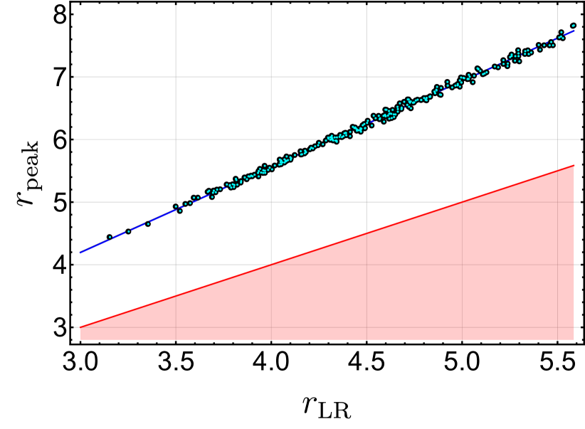
Figure 1: Distribution of values for $r_{\text{peak}}$ vs. $r_{\text{LR}}$ for 250 points chosen from the $\{q,\Lambda_{A},\Lambda_{B}\}$ parameter space. The black dots represent data obtained using the TEOBResum model of Ref. Nagar et al. (2018) dubbed GSF2⁽⁺⁾nm in Table 1. The data for the cyan (light colored) points are obtained by augmenting this TEOBResum with $\hat{A}^{(3+)}+\hat{A}^{(2-)}$ (GSF23⁽⁺⁾PN^(-)). As $r_{\text{LR}}$ is determined by finding the maximum of $r^{-2}A^{\text{NNLO}}(r)$ (see text) the resulting values for $r_{\text{LR}}$ are the same regardless of how we augment TEOBResum. However, the values of $r_{\text{peak}}$ do differ slightly, but this is not easily discernible in this plot, which is why the 250 cyan points appear to lie exactly on top of the 250 black points. The linear fit is given by $r_{\text{peak}}\approx 1.37r_{\text{LR}}+0.09$. The red region is the forbidden zone corresponding to $r_{\text{peak}}\leq r_{\text{LR}}$.

The TEOBResum model of Ref. Bernuzzi et al. (2015) employs PN series for all the tidal potentials with the exception of $(2+)$ for which the GSF series of Ref. Bini and Damour (2014) is adopted with $p=4$. Additionally, as explained in Ref. Bernuzzi et al. (2015), TEOBResum replaces the Schwarzschild LR, $u=1/3$, with the maximum of $u^{2}A^{\text{NNLO}}$, i.e., the EOB effective photon potential. $A^{\text{NNLO}}(u)$ is the EOB potential in which the point-mass $A_{0}$ potential is added to the tidal $A_{\text{T}}$ potential containing only the PN series for the $(2+),(3+),(4+)$ tidal terms (see Ref. Bernuzzi et al. (2015) and Sec. IIIA of Ref. Nagar et al. (2018)).

Following then Ref. Bernuzzi et al. (2015) to obtain the complete tidal potential we have to finally replace the denominators $(1-3u)$ in Eq. (II.1) with $(1-r_{\text{LR}}^{\rm NNLO}u)$, where $r^{\rm NNLO}_{\text{LR}}$ corresponds to the peak of $u^{2}(A_{0}+A_{T}^{\text{NNLO}}(u))$. Such a new GSF-resummed potential will then yield a different effective light-ring, defined this time as the peak of $u^{2}(A_{0}+A_{T}^{\text{GSF*}}(u))$, where $A_{T}^{\text{GSF}*}$ indicates any tidal potential with GSF-resummed information. Clearly, one has to a posteriori check that the so constructed dynamics never passes through $r_{\text{LR}}^{\rm NNLO}$ in the physically meaningful region. To do so easily, we can monitor the behavior of the orbital frequency and identify the radius where it peaks. This point $r_{\text{peak}}$, is close to the peak of the $\ell=m=2$ waveform amplitude that we conventionally identify as the merger point. In Fig. 1 we plot $r_{\text{peak}}$ vs. $r_{\text{LR}}$ for 250 points in the $\{q,\Lambda_{A},\Lambda_{B}\}$ parameter space for TEOBResum of Ref. Bernuzzi et al. (2015) and TEOBResum supplied with (3+) and (2-) tides as GSF series. The figure illustrates that the EOB radial separation never hits the $r_{\rm LR}^{\rm NNLO}$ effective light ring location. With our new GSF series for the $(2-),(3+)$ potentials we now have several different options to flex the original TEOBResumS model. We show some of our main choices in Fig. 2, where the legend is explained in Table 1.

Our final addition to TEOBResum regards the tidal contribution $B_{\text{T}}(u)$ to the EOB $B$ potential in the EOB Hamiltonian. From Ref. Vines and Flanagan (2010), one has that the contribution that is added to the PN-expanded point-mass part of the potential $B_{0}$ is

$$B_{\text{T}}(u)=3\kappa_{2}^{T}(3-5\nu)u^{6}\ .$$ (30)

To incorporate this information within TEOBResum we need first to review the choices previously made. In particular, let us remember that the current $B$ function is defined as $B\equiv D/A$, where the $D$ function is the 3PN-accurate one that is resummed as a Padé (0,3) approximant as $D\equiv(1+6\nu u^{2}-2(3\nu-26)\nu u^{3})^{-1}$, and $A\equiv A_{0}+A_{T}$, i.e., the total potential as a sum of the point-mass with the tidal part. As a consequence, the $B$ function obtained in this way already incorporates the tidal contribution, that is, however, inconsistent, once PN-expanded, with Eq. (30). There are several ways to overcome this difficulty and have the correct PN-expansion of the tidal $B$ potential. The simplest is just to add to the current $B$ potential a term $B^{\prime}_{\rm T}(u)$ such that the term proportional to $\kappa_{2}^{T}$ of the PN-expanded $B+B^{\prime}_{\rm T}$ coincides with Eq. (30). This condition yields

$$B_{\rm T}^{\prime}(u)=\kappa_{2}^{T}(8-15\nu)u^{6}\,.$$ (31)

We shall investigate the effect of this additional term on phasing in Sec. III below.

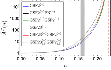
Figure 2: A sample of tidal EOB potentials at our disposal shown against each other for $q=1$, $\Lambda=1531.34$ corresponding to $\kappa_{2}^{T}=287.126$. The vertical gray region marks the various values for $r_{\text{peak}}$ at which the orbital frequency peaks for each EOB variant plotted here. See Table 1 for explanation of the legend labels. The vertical red dashed line marks the location of the NNLO effective light ring, $u_{\text{LR}}^{\rm NNLO}\approx 0.228$, for this set of parameters. The vertical gray dotted line marks the Schwarzschild LSO at $u=1/6$. As the relative contribution of the $(2-)$ tides is $\lesssim\mathcal{O}(10^{-2})$, the potentials with $(2-)$ tides overlap rather well with their no-$(2-)$ counterparts. Therefore, to distinguish these, we opted to plot them over limited domains as shown by the solid black, green, and red curves with the black curve under the green one. Note that the dashed, gray, line corresponds to the potential with $p=4$ replaced by $p=4.5$, in order to appreciate the sensitivity to this parameter.

II.2 Tidal Waveform

When including the effects of the tides on the waveform, the point-mass waveform $h^{0}_{\ell m}$ is augmented via Damour et al. (2012a)

$$h_{\ell m}=h^{0}_{\ell m}+h^{T}_{\ell m}=h^{\text{Newt}}_{\ell m}\,(\hat{h}^{0}_{\ell m}+\hat{h}_{\ell m}^{T}),$$ (32)

with the general expression for $h^{\text{Newt}}_{\ell m}$ given, e.g., by Eq. (18) of Ref. Damour et al. (2013) modulo normalization and sign conventions. Until recently, only the $(2+)$ NLO contribution to $\hat{h}^{T}_{22}$ was known Vines et al. (2011), but thanks to Ref. Banihashemi and Vines (2018), we now have access to all the NLO information for the $(2+)$ contributions to $\hat{h}^{T}_{21},\hat{h}^{T}_{31},\hat{h}^{T}_{33}$ as well as the $(2+)$ LO contribution to $\hat{h}^{T}_{32}$, and the LO $(2-)$ contributions for $\ell\leq 3,m\leq\ell$. We adopt all of this new information to all our tidal choices for TEOBResum with one exception which we label by “nm” (no multipoles) in Table 1 and Fig. 5.

Rewriting the results for $\hat{h}^{T}_{\ell m}$ from Appendix A of Ref. Banihashemi and Vines (2018) in our own notation, and using $X_{B}=1-X_{A}$, we obtain

$$\hat{h}_{22}^{\rm T} =\kappa_{A}^{(2+)}\left(\frac{3-2X_{A}}{1-X_{A}}\right)x^{5}+\biggl{[}\frac{14}{9}\kappa_{A}^{(2-)}-\kappa_{A}^{(2+)}\frac{\left(202-560X_{A}+340X_{A}^{2}-45X_{A}^{3}\right)}{42(1-X_{A})}\biggr{]}x^{6}+(A\leftrightarrow B),$$ (33)

$$\hat{h}_{21}^{\rm T} =\biggl{[}\kappa_{A}^{(2+)}\left(-\frac{9}{2}+6X_{A}\right)-\kappa_{A}^{(2-)}\frac{1}{2(1-X_{A})}\biggr{]}x^{5}-(A\leftrightarrow B),$$ (34)

$$\hat{h}_{33}^{\rm T} =-6\,\kappa_{A}^{(2+)}(1-X_{A})x^{5}+\biggl{[}\,\kappa_{A}^{(2+)}\left(21-\frac{89}{2}X_{A}+\frac{55}{2}X_{A}^{2}-5X_{A}^{3}\right)+\frac{1}{2}\kappa_{A}^{(2-)}(9X_{A}-5)\biggr{]}x^{6}-(A\leftrightarrow B),$$ (35)

$$\hat{h}_{32}^{\rm T} =\biggl{[}4\,\kappa_{A}^{(2+)}(2-4X_{A}+3X_{A}^{2})+\frac{4}{3}\kappa_{A}^{(2-)}\biggr{]}x^{5}+(A\leftrightarrow B),$$ (36)

$$\hat{h}_{31}^{\rm T} =-6\,\kappa_{A}^{(2+)}(1-X_{A})x^{5}+\biggl{[}\,\kappa_{A}^{(2+)}\left(1+\frac{5}{6}X_{A}-\frac{131}{6}X_{A}^{2}+\frac{65}{3}X_{A}^{3}\right)+\frac{1}{2}\kappa_{A}^{(2-)}(17X_{A}-13)\biggr{]}x^{6}-(A\leftrightarrow B).$$ (37)

Note that some of the $(A\leftrightarrow B)$ terms are preceded by a minus sign. This PN-expanded tidal part is then incorporated in the TEOBResum following Appendix A of Ref. Damour et al. (2012a), in particular with the tail factor factorized in front of the tidal waveform contribution as above. As usual in EOB models, the PN variable $x$ is replaced by the EOB velocity variable $v_{\Omega}=r_{\Omega}\Omega$, where $r_{\Omega}=r\psi^{1/3}$ and $\psi$ is computed using the EOB Hamiltonian Damour and Gopakumar (2006); Damour and Nagar (2010).

III Effect of enhanced analytical information on GW phasing

In this section we evaluate the impact, in terms of accumulated GW phase, of the new analytical information discussed above. In particular we separately focus on the effect of the GSF-resummed $\ell=3$ potential and on all other contributions (gravitomagnetic effects and additional tidal corrections to waveform amplitude etc.) that turn out to be largely subdominant. The key options for the models investigated here are summarized in Table 1. For example, GSF23⁽⁺⁾GSF2^(-) represents TEOBResum employing $(2\pm),(3+)$ GSF-resummed tides, with our standard choice $p=4$. Finally, we also mention the possibility of flexing $p$, with the subscript $4.5$ representing the choice $p=9/2$. The default, or baseline, TEOBResum model that is used as benchmark for our comparisons is GSF2⁽⁺⁾.

Shortname	$\hat{A}^{(2+)}$	$\hat{A}^{(3+)}$	$\hat{A}^{(2-)}$	$p$	$\hat{h}^{T}_{\ell m}$
PN(+)	PN	PN	PN	-	✓
GSF2(+)nm	GSF-R	PN	✗	4	✗
GSF2(+)	GSF-R	PN	✗	4	✓
GSF2(+)PN(-)	GSF-R	PN	PN	4	✓
GSF2(+)GSF2(-)	GSF-R	PN	GSF-R	4	✓
GSF23(+)	GSF-R	GSF-R	✗	4	✓
GSF23(+)PN(-)	GSF-R	GSF-R	PN	4	✓
GSF23(+)GSF2(-)	GSF-R	GSF-R	GSF-R	4	✓
GSF23${}^{\rm(+)}_{4.5}$GSF2${}^{\rm(-)}_{4.5}$	GSF-R	GSF-R	GSF-R	4.5	✓

Table 1: Summary of the key analytical terms and components of TEOBResum tested in this work. GSF-R and PN stand for “GSF resummed” and post-Newtonian expressions described in Sec. II.1. All models include the $B_{\text{T}}$ term of Eq. (30), which is individually tested in Fig. 6. All models except GSF2⁽⁺⁾nm include the waveform multipoles described in Sec. II.2. For example, GSF2⁽⁺⁾PN^(-) represents the EOB model in which the $(2+)$ tide is modelled as a GSF series and the $(2-)$ tide as a PN series.

III.1 Impact of the $\ell=3$ GSF-resummed potential

Let us start by investigating the impact of the GSF-resummed $\ell=3$ contribution to the tidal potential. Its effect is to make the EOB $A$ potential more negative (i.e., more attractive) with respect to the corresponding PN-expanded NNLO $\ell=3$ part, so that the binary inspirals faster up to merger. Figure 3 shows the effect of the $\ell=3$ 1GSF and 2GSF terms individually, where we employed three equal-mass BNS configurations: SLy, H4, and MS1b with $\kappa_{2}^{T}=73.53,191.4$, and $289.6$, respectively. We recall that the 1GSF and 2GSF terms come from Eq. (II.1) above, with $r_{\rm LR}$ of the Schwarzschild geometry replaced by the corresponding EOB one of the NNLO tidal potential, and having fixed $p=4$. The figure shows the phase difference versus GW frequency $M\omega_{22}$. Note that the curves end at the peak values of $M\omega_{22}$, which approximately correspond to the peak of the $(2,2)$ waveform mode amplitude that was found to be rather close and consistent with the merger frequency coming from NR simulations Bernuzzi et al. (2015). The figure illustrates the contribution of each term to the total $(2,2)$-mode phase of a baseline tidal model consisting of only the $\ell=2$ 0GSF, 1GSF terms (no $\ell>2$ tides whatsoever).

Note that, the phase accumulation due to the new terms starts very late in the inspiral, $M\omega_{22}\gtrsim 0.06$, consistent with the fact that the $\ell=3$ GSF-resummed potential becomes distinguishable only in the last few cycles before the merger as can be seen by comparing the brown and blue curves in Fig. 2. Overall, we see that the first-order $\ell=3$ GSF term contributes up $\mathcal{O}(1)$ radian and the second-order term up to roughly 4 radians.

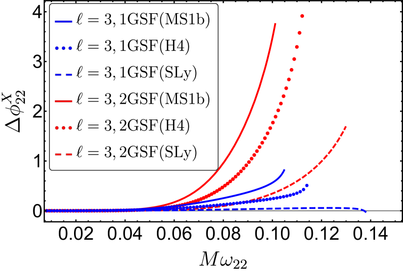
Figure 3: The effect of the 1GSF and 2GSF $\ell=3$ terms on the $(2,2)$ mode phase. Here, $\Delta\phi^{X}_{22}\equiv\phi^{b}_{22}-\phi^{X}_{22}$, where $\phi_{22}^{b}$ is the phase of the baseline BNS run that contains only the $\ell=2$ 0GSF, 1GSF terms for tides. We then add to this base either the 1GSF or 2GSF $\ell=3$ tides and re-evolve the inspiral to obtain the corresponding $\phi_{22}^{X}$. We used $\kappa_{2}^{T}=73.53,191.4,289.6$ for the SLy, H4, MS1b EOS, respectively.

Having gained a quantitative understanding of the impact of the separate $\ell=3$ GSF-resummed contributions to the potential, we incorporate them, Eq. (II.1), into TEOBResum, thus replacing the previously used PN series truncated at NNLO. According to the summary of the various terms listed in Table 1, we name this flavor of the model GSF23⁽⁺⁾. We gauge its effect on the $(2,2)$ phase by comparing it to the phase resulting from the GSF2⁽⁺⁾ model which will serve as our standard baseline for the remainder of this article unless otherwise noted. We show the resulting phase differences, $\Delta\phi_{22}^{X}\equiv\phi_{22}^{\text{GSF{2}${}^{\rm(+)}$}}\!\!-\phi^{X}_{22}$, in Fig. 4 for three equal-mass configurations: $\{\text{EOS},q,\Lambda\}=\{\text{SLy},1,392.151\},\{\text{ALF2},1,733.323\},\{\text{MS1b},1,1544.53\}$, and MS1b with $q=1.5,\Lambda_{A}=1099.9,\Lambda_{B}=4391.144$ translating to $\kappa_{2}^{T}=73.53,137.5,289.6$, and $373.4$, respectively. As GSF23⁽⁺⁾ is more attractive than GSF2⁽⁺⁾, because of the stronger $\ell=3$ contribution, it plunges faster, it accumulates less phase, and therefore $\Delta\phi_{22}^{X}$ is positive. Also note, in passing, that the merger frequency decreases as $\kappa_{2}^{T}$ increases because of the correspondingly augmented tidal interaction Bernuzzi et al. (2014).

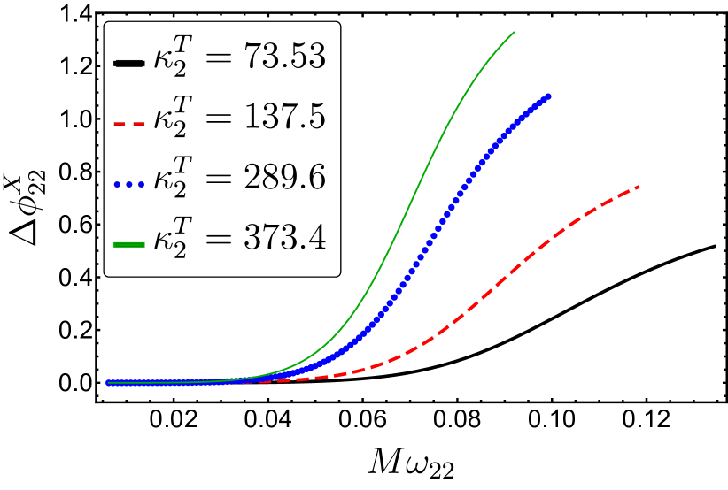
Figure 4: The effect of the entire GSF-resummed $\ell=3$ contribution, model GSF23⁽⁺⁾, on the $(2,2)$-waveform phase as compared with respect to the phase of the baseline GSF2⁽⁺⁾ model. Here, $\Delta\phi_{22}^{X}\equiv\phi_{22}^{\text{GSF{2}${}^{\rm(+)}$}}\!\!-\phi^{X}_{22}$. As $\kappa_{2}^{T}$ increases, the phase difference grows corresponding to the tides becoming more attractive, thus the neutron stars merge sooner.

III.2 Impact of all other tidal contributions

As detailed in Sec. II we have added the gravitomagnetic tidal interaction to TEOBResum either as a PN series or a GSF-resummation. We have additionally augmented the EOB $B$ potential and the multipolar waveforms with new analytical tidal information. The contribution of these new terms are subdominant compared to the $\ell=3$ GSF-resummed tide. Their effects on the evolution of the GW phase is shown in Fig. 5 once again in terms of $\Delta\phi_{22}^{X}\equiv\phi_{22}^{\text{GSF{2}${}^{\rm(+)}$}}\!\!-\phi^{X}_{22}$. As $\Delta\phi^{X}_{22}$ varies in sign and over several orders of magnitude, we opted to display $|\Delta\phi^{X}_{22}|$ as semilog plots in the figure, where the four panels correspond to the same four cases chosen for Fig. 4. In the following subsections, we discuss the effects of these subdominant terms.

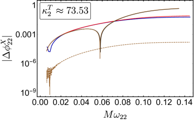
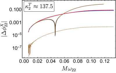
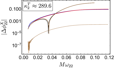
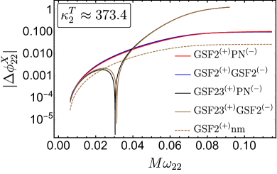
Figure 5: The phase difference $\Delta\phi^{X}_{22}\equiv\phi_{22}^{\text{GSF{2}${}^{\rm(+)}$}}\!\!-\phi^{X}_{22}$, between the baseline TEOBResum model, GSF2⁽⁺⁾, and various tidally augmented TEOBResum variants listed in Table 1. Starting from the upper-left panel and going clockwise, we have $\{\text{EOS},q,\Lambda\}=\{\text{SLy},1,392.151\},\{\text{ALF2},1,733.323\},\{\text{MS1b},1,1544.53\}$. The lower-right panel corresponds to MS1b with $q=1.5,\Lambda_{A}=1099.9,\Lambda_{B}=4391.144$. The blue and the red curves are negative because the gravitomagnetic Love number $\Sigma$ is negative for irrotational fluids. The sign change of the GSF23⁽⁺⁾ curves (brown and black) is explained in the text.

III.2.1 Gravitomagnetic tides: irrotational fluids

Since the gravitomagnetic Love number is negative, the contribution of the $(2-)$ tide, whether as a PN or GSF series, yields $\Delta\phi_{22}<0$. This is in concordance with our physical intuition if we recall that the overall sign of the tidal potential is negative. Hence, gravitomagnetic terms make it less negative thus extending the inspiral time and increasing the accumulated phase which, when subtracted from the smaller phase of GSF2⁽⁺⁾, expectedly yields a negative number.

We see in Fig. 5 that the contribution of the negative gravitomagnetic terms (red, blue curves) to the phase is $\lesssim 0.1$ radian up to the EOB mergers given roughly by $0.12\lesssim M\omega_{22}\lesssim 0.14$ depending on $\kappa_{2}^{T}$. Moreover, the difference between using PN vs. GSF series for the $(2-)$ tides is almost indistinguishable as can be seen both in the GSF2⁽⁺⁾ (red vs. blue curves) and GSF23⁽⁺⁾ cases (black vs. brown curves). Note that the sign change of the black, brown curves in Fig. 5 is due to the sign change in the corresponding tidal potential ${A}^{(2-)}+{A}^{(3+)}$ because these terms have opposite signs and different weak-field behavior ($u^{7}$ vs. $u^{10}$, respectively). Even less distinguishable than the gravitomagnetic contribution is the effect of augmenting the waveform by adding the $(2+)$NLO and $(2-)$LO terms to $\hat{h}^{T}_{22}$. This effect is represented by the dashed brown curves labelled GSF2⁽⁺⁾nm and amounts to at most $\sim 0.02\,$radian.

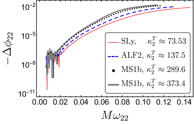
Figure 6: The effect of augmenting the $B$ potential with the tidal term $B^{\prime}_{\text{T}}$ of Eq. (31) on the GW phase $\phi_{22}$ for the four cases of Fig. 5. In each case, the phase difference is computed with respect to the baseline model GSF2⁽⁺⁾ (see Table 1). Note that we plot $-\Delta\phi_{22}$. See Sec. III.2.3 for why $\Delta\phi_{22}$ is negative in this comparison.

BAM	EOS	$\kappa_{2}^{T}$	$m_{A}~{}[M_{\odot}]$	$q$	$\Lambda_{A}$	$\Lambda_{B}$	$k_{A}^{(2)}$	$k_{B}^{(2)}$	$\mathcal{C}_{A}$	$\mathcal{C}_{B}$	$\Sigma_{A}$	$\Sigma_{B}$	$j_{A}^{(2)}$	$j_{B}^{(2)}$	Ref.
0011	ALF2	72.12	1.500	1.000	384.7	384.7	0.1044	0.1044	0.1784	0.1784	$-3.775$	$-3.775$	$-0.03278$	$-0.03278$	Dietrich et al. (2017a)
0095	SLy	73.53	1.350	1.000	392.2	392.2	0.09333	0.09334	0.1738	0.1738	$-3.823$	$-3.823$	$-0.02911$	$-0.02911$	Dietrich et al. (2017a)
0127	SLy	78.05	1.650	1.503	1371.	93.45	0.1172	0.06433	0.1416	0.2150	$-8.761$	$-1.553$	$-0.02398$	$-0.03421$	Dietrich and Hinderer (2017); Dietrich et al. (2017b)
0017	ALF2	132.7	1.650	1.500	2218.	196.6	0.1443	0.08692	0.1341	0.1967	$-12.17$	$-2.460$	$-0.02533$	$-0.03480$	Dietrich et al. (2017a)
0107	SLy	136.6	1.354	1.224	1320.	383.9	0.1174	0.09288	0.1427	0.1744	$-8.542$	$-3.770$	$-0.02430$	$-0.02919$	Dietrich et al. (2018b)
0021	ALF2	139.6	1.750	1.750	122.3	3528.	0.07505	0.1517	0.2101	0.1234	$-1.830$	$-16.78$	$-0.03596$	$-0.02309$	Dietrich et al. (2017a)
0037	H4	191.4	1.372	1.000	1020.	1021.	0.1140	0.1140	0.1494	0.1494	$-7.181$	$-7.182$	$-0.02567$	$-0.02567$	Dietrich et al. (2017a)
0048	H4	192.8	1.528	1.250	1990.	500.2	0.1262	0.09762	0.1334	0.1671	$-11.30$	$-4.478$	$-0.02293$	$-0.02797$	Dietrich et al. (2017a)
0058	MPA1	115.3	1.350	1.000	614.9	614.9	0.1120	0.1120	0.1648	0.1648	$-5.128$	$-5.128$	$-0.02988$	$-0.02988$	Dietrich et al. (2017a)
0094	MS1b	250.2	1.944	2.059	9249.	183.7	0.1619	0.08698	0.1031	0.1994	$-33.14$	$-2.358$	$-0.01855$	$-0.03572$	Dietrich et al. (2017b, 2015)
0091	MS1b	280.4	1.650	1.500	502.2	4391.	0.1099	0.1525	0.1709	0.1183	$-4.490$	$-19.56$	$-0.03143$	$-0.02173$	Dietrich and Hinderer (2017); Dietrich et al. (2017b)
0064	MS1b	289.6	1.350	1.000	1542.	1546.	0.1347	0.1347	0.1422	0.1422	$-9.492$	$-9.508$	$-0.02653$	$-0.02651$	Dietrich et al. (2017a)

Table 2: The initial configuration for the BAM and EOB runs that we use for the EOBNR comparisons. Note $q\equiv m_{A}/m_{B}>1$ and the numbers for the BAM NR runs are approximate as they are extracted from NR initial data. See Sec. II.1 for the notation.

BAM	$\hat{\omega}^{\text{mrg}}$	$f^{\text{mrg}}$(Hz)	$j^{\text{mrg}}$	$E_{b}^{\text{mrg}}$
0011	0.1615	1739	3.358	$-0.06302$
0095	0.1711	2048	3.318	$-0.06520$
0127	0.1364	1604	3.404	$-0.05969$
0017	0.1197	1406	3.532	$-0.05388$
0107	0.1333	1750	3.489	$-0.05592$
0021	0.1075	1263	3.584	$-0.05151$
0037	0.1357	1598	3.516	$-0.05467$
0048	0.1168	1371	3.568	$-0.05213$
0058	0.1486	1778	3.451	$-0.05804$
0094	0.08877	993	3.700	$-0.04686$
0091	0.1014	1191	3.658	$-0.04864$
0064	0.1234	1477	3.612	$-0.05068$

Table 3: BAM merger (mrg) data. The merger is taken to occur at the peak of the amplitude of the $\ell=m=2$ mode. $f$ is the corresponding quadrupole GW frequency in Hz. $j$ is the angular momentum and $E_{b}$ the binding energy (IV.1).

III.2.2 Gravitomagnetic tides: static fluid

For the sake of comparison, we also considered gravitomagnetic tides for static fluids. As a generic difference, we note that static gravitomagnetic Love numbers are positive as opposed to irrotational ones, and, for polytropes, their absolute values are about twice those of irrotational Love numbers (see Fig. 1 of Ref. Landry and Poisson (2015)). For realistic EOS, we obtain the static Love numbers from the quasi-universal relations of Ref. Jimenez-Forteza et al. (2018) which yield $\Sigma_{\text{stat}}\sim 2|\Sigma|$, roughly in agreement with the polytropic ratio mentioned above. As a result, we would expect static Love numbers to result in phase differences that are roughly twice the magnitude of $\Delta\phi^{\text{red,blue}}_{22}$ of Fig. 5 and with a positive sign. Repeating the runs of Fig. 5 for GSF2⁽⁺⁾PN^(-) and GSF2⁽⁺⁾GSF2^(-) with $\Sigma_{\text{stat}}$, we indeed find that $\Delta\phi_{22}$ now accumulates up to $\sim 0.2$ radian at the EOB merger ($0.12\lesssim M\omega_{22}\lesssim 0.14$), but has, as expected, the opposite sign to the irrotational case.

We opt for irrotational Love numbers because we think they represent more realistic scenarios: in Ref. Landry and Poisson (2015), Landry and Poisson studied gravitomagnetic tidal interactions relaxing the hypothesis that the NS fluid be in hydrostatic equilibrium. Instead, they considered fluids in an irrotational state, thus allowing for internal currents induced by gravitomagnetic tidal fields. It was only recently shown Pani et al. (2018) that the independent formalism for relativistic tides in Ref. Damour and Nagar (2009a) by Damour and Nagar indeed implicitly enforces the fluid to an irrotational state and is equivalent to the Landry-Poisson formulation. Here we follow the Damour-Nagar conventions for Love numbers as shown in Sec. II.1.

III.2.3 Leading-order tidal term in the EOB $B$ potential

The consequence of augmenting the $B$ potential by $B_{\text{T}}^{\prime}$ of Eq. (31) is shown in Fig. 6, once again in terms of $\Delta\phi^{X}_{22}$ where $X$ now represents GSF2⁽⁺⁾ augmented with $B^{\prime}_{\text{T}}$. We show the phase difference again for four points in $\{q,\Lambda_{A},\Lambda_{B}\}$ space with increasing $\kappa_{2}^{T}$. Even for very large $\kappa_{2}^{T}$, the effect of the $B^{\prime}_{\text{T}}$ term on the phase of the waveform is too small to matter for the current generation of ground-based detectors. Note that, unlike in Fig. 5, $\Delta\phi_{22}$ is now negative because $\dot{r}\propto B^{-1/2}$ (cf. Eq. (6b) of Ref. Damour et al. (2013)). Hence increasing $B$ decreases $\dot{r}$, thus lengthening the inspiral time. The $B_{\text{T}}^{\prime}$ term has been added to all models of Table 1.

IV EOB/NR comparisons: energetics and waveforms

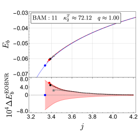
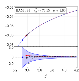
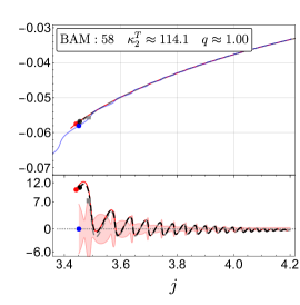
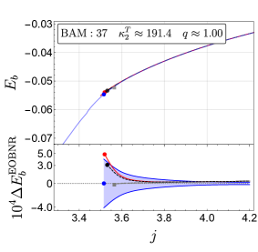
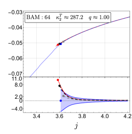
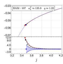
Figure 7: EOB-NR comparison in terms of binding energy as a function of angular momentum for the $q=1$ binaries of Table 2 and the $q\approx 1.22$ case. In each subfigure, the upper panel shows the TEOBResum $E_{b}(j)$ curves for three different models listed in Table 1 (solid red, dashed black and dashed gray) along with the corresponding NR data represented by the solid blue curves. The dots and the squares mark the peak orbital frequency of each run with the corresponding color. The values for NR $E_{b}$ and $j$ at the merger are listed in Table 3. Lower panel of each subfigure shows the difference between EOB and NR results, $\Delta E_{b}^{\text{EOBNR}}\equiv E_{b}^{\text{EOB}}-E_{b}^{\text{NR}}$, with the shaded regions representing our estimation of the NR error. The blue error regions are more reliable because they come from convergent simulations, while the pink ones are obtained from differences between the two highest NR resolutions, thus are less certain (cf. Sec. IV). Note that we amplify the error region by a factor of $10^{4}$ to improve its visibility. The oscillations in the panel for BAM:0058 are due to residual eccentricity.

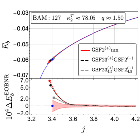
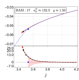
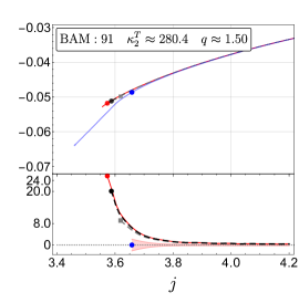
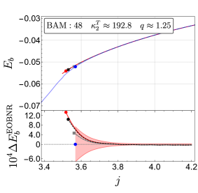
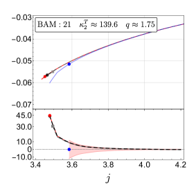
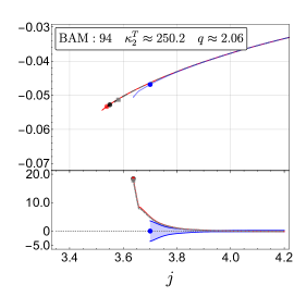
Figure 8: Same as Fig. 7 but for binaries with $q\gtrsim 1.25$ with the top panels showing the $q\approx 1.5$ cases. The error regions for BAM:0017, 0021, 0048, 0091, 0127 are less certain thus have been shaded in light pink.

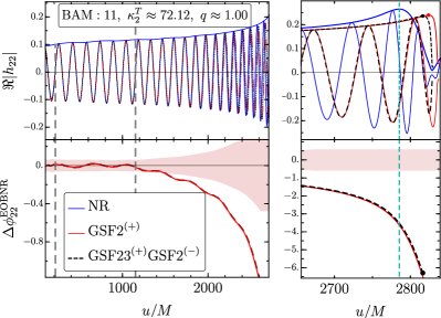
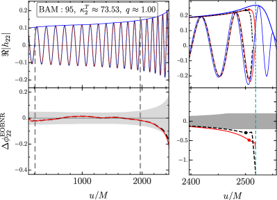
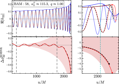
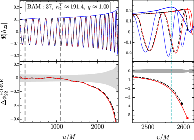
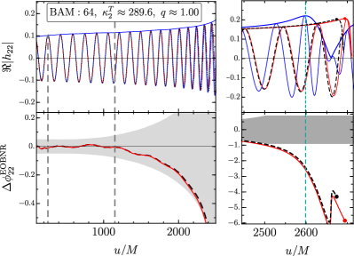
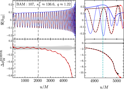
Figure 9: Dephasing between BAM NR simulations and two TEOBResum variants for $q\approx 1$ in terms of increasing $\kappa_{2}^{T}$. We also included the $q\approx 1.224$ BAM:0107 EOBNR comparison here. The NR waveforms and amplitudes are plotted as solid blue curves. The TEOBResum variants plotted are: GSF2⁽⁺⁾ (red) and GSF23⁽⁺⁾GSF2^(-) (dashed black). In each subfigure, upper-left panels show the waveforms starting from $\hat{\omega}\sim 0.03-0.04$ corresponding roughly to ($M_{\odot}/M$) kHz. Upper-right panels show roughly the last cycle before and after the NR merger. The lower panels display the phase disagreement $\Delta\phi_{22}^{\text{EOBNR}}\equiv\Delta\phi_{22}^{X}-\Delta\phi_{22}^{\text{NR}}$ with $X$ representing the two TEOBResum variants. The shaded (pink or gray) regions represent our estimated NR phase error. The vertical cyan dashed lines mark the peak of NR waveform amplitude. The red, green, blue dots respectively represent the same for the three TEOBResum variants listed above. The vertical, dashed gray lines mark the waveform alignment interval $I_{\omega}=(\hat{\omega}_{L},\hat{\omega}_{R})$ introduced in Sec. IV.2.

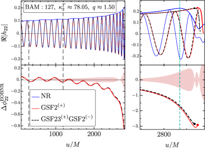
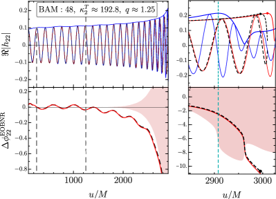
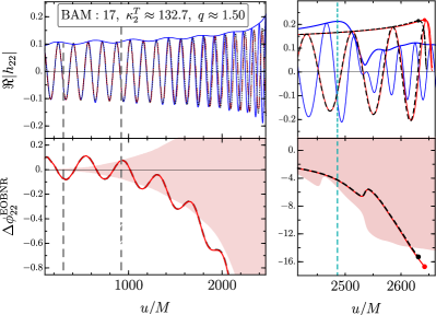
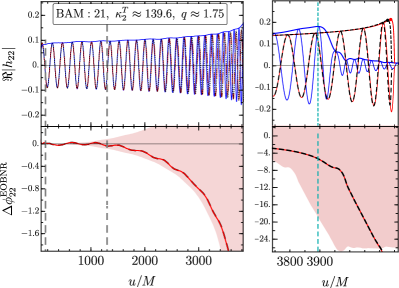
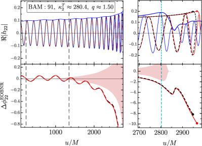
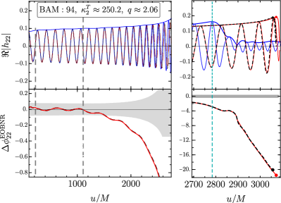
Figure 10: Same as Fig. 9, but for the $q\gtrsim 1.25$ cases. The figures in the left column correspond to $q\approx 1.50$ in terms of $\kappa_{2}^{T}$ increasing downward. See the caption of Fig. 9 for details.

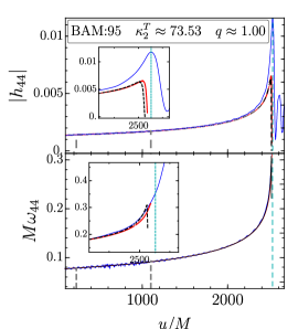
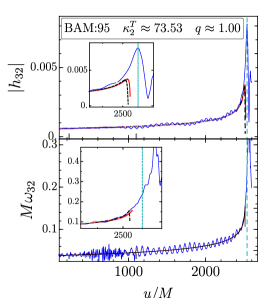
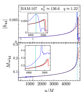
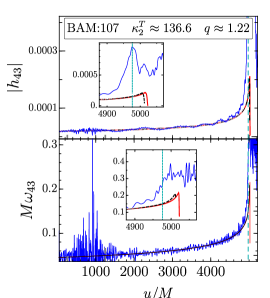
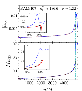
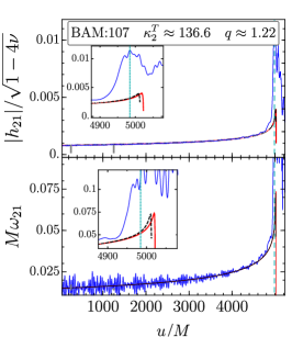
Figure 11: EOB-NR comparisons for higher multipoles. See Fig. 9 for legend. Upper panels of each subfigure show the amplitudes of the aligned EOB variants against the corresponding NR waveform amplitude. The lower panels show the dimensionless frequencies $M\omega_{\ell m}$ from the NR and the EOB data. The insets show data near the NR merger. For modes with the smallest amplitudes, the noise in the NR data is clearly visible.

We assess the new analytical results against NR data from the public database of the CoRe collaboration Dietrich et al. (2018a). The employed datasets are summarized in Table 2 and cover a relevant range of EOS, masses and mass ratios. Most of the NR data consist of the eccentricity-reduced, error-controlled waveforms computed in Ref. Dietrich et al. (2017a). Note that much of the data employed here are of higher quality than those employed in Ref. Bernuzzi et al. (2015) to verify the performance of TEOBResum. As a consequence, the newest data enable a more detailed assessment of the analytical EOB model than previously done. We also include simulations from Refs. Dietrich et al. (2015, 2017b); Dietrich and Hinderer (2017) in order to explore mass ratios significantly different from $q=1$. Roughly half of our chosen data sets show clear convergence with grid resolution and allow us to compute consistently the error budget Bernuzzi et al. (2012b); Bernuzzi and Dietrich (2016). The rest, specifically the BAM:0011, 0017, 0021, 0048, 0058, 0091, 0127 runs, do not show robust convergence and do not allow us to compute consistent error bars for the phase. Following the above references, the error from these data sets is estimated as the difference of the two highest resolutions and shown using pink shading in Figs. 7 through 10. Therefore, the comparisons with these data sets cannot be considered conclusive. Nonetheless, we present EOB-NR comparisons for all twelve cases with the double aim of (i) suggesting possible limitations of the analytical model and (ii) indicating a possible direction for improving current NR simulations.

IV.1 Energetics

EOB and NR dynamics are compared by considering the gauge-invariant relation between binding energy per reduced mass, $E_{b}=(E-M)/(M\nu)$ and orbital angular momentum $j\equiv p_{\varphi}$ Damour et al. (2012b); Bernuzzi et al. (2012a, 2015). We recall that in the EOB case $E$ is just the Hamiltonian function computed along the EOB dynamics. For the NR configurations, $(E^{\rm NR},j^{\rm NR})$ is obtained as detailed in Damour et al. (2012b); Bernuzzi et al. (2012a). Figure 7 collects several $q=1$ configurations with increasingly larger tidal interaction, as well as a $q=1.22$ case. We display $1.25\lesssim q\lesssim 2$ cases in Fig. 8. In each subfigure, the bottom panels show $\Delta E_{b}^{\text{EOBNR}}\equiv E_{b}^{\text{EOB}}-E_{b}^{\text{NR}}$ with the shaded region representing our estimated NR error. We recall that the blue-shaded regions come from convergent simulations, while the pink-shaded regions are obtained as difference between the two highest resolutions. For the purposes of relating our results to that of Ref. Nagar et al. (2018), we show GSF2⁽⁺⁾nm as the solid red curves. On both the NR and EOB curves, the markers indicate the conventional merger points, i.e., the values corresponding to the peak of the amplitude of the $\ell=m=2$ waveforms. The black dashed curves terminating at the black dots represent GSF23⁽⁺⁾GSF2^(-), while the dashed gray curves terminating at the gray squares represent GSF23${}^{\rm(+)}_{4.5}$GSF2${}^{\rm(-)}_{4.5}$ to illustrate the sensitivity of this quantity on the choice of the value of the exponent $p$.

The performances of the analytical models are in broad agreement with NR within their errors, but agreement in the $j$-interval corresponding to the last few cycles up to merger depends on the value of $\kappa_{2}^{T}$. Let us focus first on Fig. 7. As a general statement, the, already good, EOB/NR agreement yielded by the GSF2⁽⁺⁾ model is even improved when the $(3+)$-GSF resummed physical information is considered, i.e. with the GSF23⁽⁺⁾GSF2^(-) variant. The latter predicts a conventional merger point occurring at slightly lower values of $j$ than the previous case though, especially when $\kappa_{2}^{T}$ is increased, it gets closer to the NR prediction. This seems to be a robust conclusion driven by inspecting the lower panels of Fig. 7, where it was possible to obtain robust error bars for NR run. Same conclusion holds true, for the same configurations, for the values of $E_{b}^{\rm mrg}$ (see especially BAM:0064 and BAM:0107). By contrast, the variant GSF23${}^{\rm(+)}_{4.5}$GSF2${}^{\rm(-)}_{4.5}$ systematically predicts values of the angular momentum at conventional merger that are systematically larger than the NR ones.

Figure 7 ($q\approx 1$) shows that our $p=4$ GSF-resummed tidal models go from slightly overestimating the tidal interaction to slightly underestimating it as $\kappa_{2}^{T}$ grows. This means that there is a certain region, $100\lesssim\kappa_{2}^{T}\lesssim 200$, where the energetics yielded by GSF23⁽⁺⁾ agrees rather well with the NR one. This region corresponds to moderately stiff EOS with $500\lesssim\Lambda\lesssim 1000$ which translates to ${500\lesssim\tilde{\Lambda}\lesssim 2200}$ using, e.g., the low-spin prior inferred mass ratio, $q\in[1,1.37]$ of GW170817 Abbott et al. (2018b). Our region has some overlap with the LIGO-Virgo constraint of $\Lambda\lesssim 800$ Abbott et al. (2017, 2018a); De et al. (2018); Abbott et al. (2018b) and the one from electromagnetic counterpart, $\tilde{\Lambda}\gtrsim 400$ Radice et al. (2018).

We see a similar pattern in the top panels of Fig. 8 corresponding to $q\approx 1.5$ where the TEOBResum models overshoot the NR merger with increasing $\kappa_{2}^{T}$. However, as was the case with $q=1$, there might be a similar region of good agreement, but for $\kappa_{2}^{T}\lesssim 80$. It seems that GSF23${}^{\rm(+)}_{4.5}$GSF2${}^{\rm(-)}_{4.5}$ may be the most suitable model for when $q\gtrsim 1.25$. This could be indicative of this variant effectively accounting for the increased NS deformability of the $q>1$ situations. In order to draw more definitive conclusions, we require a larger set of NR data with robust errors. A good agreement between energetics should probably be obtained with a value of $p\sim 9/2$ for large values of $\kappa_{2}^{T}$ and slightly smaller than 4 for smaller value of $\kappa_{2}^{T}$. Since a meaningful assessment of the effective value of $p$ would require more error-controlled NR simulations, we leave such exploration to future work.

IV.2 GW Phasing

We compare the EOB and NR multipolar waveforms by using a standard (time and phase) alignment procedure in the time domain  Baiotti et al. (2010). Relative time and phase shifts are determined by minimizing the $L^{2}$ distance between the EOB and NR phases integrated on a time interval corresponding to the dimensionless frequency interval $I_{\omega}=(\hat{\omega}_{L},\hat{\omega}_{R})\approx(0.04,0.06)$. Such a choice for $I_{\omega}$ allows one to average out the phase oscillations linked to the residual eccentricity. As a consistency check, we employed two separate codes using different alignment routines. The waveforms we show in Figs. 9, 10 were agreed on by both codes.

In Fig. 9 we show several EOB $(2,2)$ waveforms aligned with NR ones for five $q\approx 1$ cases along with $q\approx 1.22$. For this comparison, we opted to include the following TEOBResum variants: GSF2⁽⁺⁾ (red) and GSF23⁽⁺⁾GSF2^(-) (dashed black). In each subfigure, the upper-left panels show the waveforms in the late inspiral stage with the upper-right panels showing the merger and the last few cycles before the merger. The lower panels display the phase disagreement between EOB and NR defined as $\Delta\phi_{22}^{\text{EOBNR}}\equiv\Delta\phi_{22}^{X}-\Delta\phi_{22}^{\text{NR}}$ with $X$ representing the different TEOBResum variants. The shaded (gray or pink) regions represent our estimated NR phase error.

Looking at Fig. 9, one notices that GSF23⁽⁺⁾GSF2^(-) behaves very similar to GSF2⁽⁺⁾, but merges slightly earlier due to increased tidal attraction. Within the moderate range of $100\lesssim\kappa_{2}^{T}\lesssim 200$, GSF23⁽⁺⁾GSF2^(-) runs seem to terminate closer to the NR merger and yield marginally smaller $\Delta\phi_{22}^{\text{EOBNR}}$ than GSF2⁽⁺⁾.

These trends appear to carry on to the $q\gtrsim 1.25$ cases, albeit with greater $\Delta\phi_{22}^{\text{EOBNR}}$ as can be seen from Fig. 10. In all these cases shown, the EOB models seem to overshoot the NR merger indicating that they underestimate the tidal attraction. The $q\approx 1.25$ case is consistent with $q\approx 1.22$ case with $\Delta\phi_{22}^{\text{EOBNR}}\approx-3\,$radians at the NR merger. Additionally, we see in the $q\approx 1.5$ comparisons that as $\kappa_{2}^{T}$ increases, EOB models diverge from the NR phase rather significantly at the merger. Overall, there is an indication that the tides might be stronger for larger $\kappa_{2}^{T}$, which could be mimicked by $p>4$ as in the model GSF23${}^{\rm(+)}_{4.5}$GSF2${}^{\rm(-)}_{4.5}$.

IV.3 GW higher multipoles

As an additional comparison, we took the best-quality subset of our NR data, namely $\{\tt{BAM:0037,0064,0091,0094,0095,0107}\}$, and compared the NR waveforms to EOB ones for higher multipolar modes beyond the quadrupole. This is an extension of the work of Ref. Bernuzzi et al. (2012a) where they made one comparison for the $(4,4)$ mode and another for $(3,2)$ in the $q=1$ case. For $q=1$, only $(3,2),(4,2),(4,4)$ modes are nonzero due to symmetry. Figure 11 presents the $(3,2)$ and $(4,4)$ modes for BAM:0095 ($q=1$) as well as $(2,1),(3,3),(4,3),(4,4)$ for BAM:0107 ($q\approx 1.22$). Among all our NR datasets, we chose, for illustrative purposes, the two where the most important higher modes are better resolved. The other NR modes (e.g., the (4,2)) are omitted as they are too noisy to allow for a meaningful comparison with the analytical models. We consider the two main TEOBResum avatars of above,  GSF2⁽⁺⁾ and GSF23⁽⁺⁾GSF2^(-). The relative time shift used is the one determined on the $\ell=m=2$ mode as above. For definiteness, the figure only reports the waveform amplitude and frequency. Note that NR errorbars are omitted from the plots for clarity.

For BAM:0095, which is probably the most reliable among our NR simulations, one finds an excellent consistency between both the EOB and NR amplitude and frequency essentially up to the conventional merger time as shown by the insets in the top-left panels of Fig. 11 representing the $(4,4)$ and $(3,2)$ modes.

For these cases, we computed $\Delta\phi^{\text{EOBNR}}_{\ell m}$ with respect to the NR merger. The dephasing of the various EOB variants for these modes is roughly consistent with the dephasing of the $(2,2)$ mode shown in Fig. 9 for BAM:0095, 0107. Note that the NR data is somewhat noisy for the $(2,1),(3,2),(4,3)$ modes; more accuracy in the NR multipoles would be necessary for further assessments. Overall, we find a robust agreement between current NR data and EOB waveforms up until the last few cycles before the merger, that corresponds to the GW frequencies currently observed. Additionally, despite the noise in the NR data, the various EOB waveforms are consistent with the NR ones, thus deliver a reliable description of the multipolar amplitudes up to a few orbits before the merger.

V Conclusions

In this article, we have investigated analytical improvements to the tidal sector of TEOBResum Bernuzzi et al. (2015); Nagar et al. (2018) for the description of quasicircular binary neutron star waveforms valid up to merger. Our main findings are summarized in the following.

New resummed gravitoelectric terms in the EOB $A$ potential.

The GSF-resummation of the leading order (LO) gravitoelectric $\ell=3$ term in the tidal EOB potential gives the largest effect on the GW phasing. For various binaries, the dephasing accumulated from $10\,$Hz is $-\Delta\phi_{22}\sim$ 0.5-3 radians.

New resummed gravitomagnetic terms in the $A$ potential.

The $\ell=2$ LO gravitomagnetic, either in PN or GSF-resummed form, term gives a smaller contribution to the GW phasing than the $\ell=3$ gravitoelectric term. In the most relevant case (stiff EOS) we find that $\Delta\phi_{22}\lesssim{0.1}$ radian from $10\,$Hz up to merger, cf. Fig. 5. The effect on the phasing is larger by of a factor $\sim\,$two and has the opposite sign if we assume that the gravitomagnetic interaction is parameterized by static Love numbers. The inclusion of gravitomagnetic terms in the Taylor F2 approximant is found to be negligible for GW data analysis of LIGO-Virgo data Jimenez-Forteza et al. (2018). Our results seem to support this conclusion, but we leave for the future a detailed assessment using TEOBResum waveforms.

Tidal correction to the $B$ potential.

The LO tidal correction to the EOB $B$ potential computed in Ref. Vines and Flanagan (2010) is positive leading to a (small) repulsive effect. Its impact on the GW is rather small and it is quantified in Fig. 6 for a sample of binaries with $|\Delta\phi_{22}|\sim 0.03$ at most.

Tidal corrections in multipolar waveform and flux.

The inclusion of the gravitoelectric and magnetic terms of Ref. Banihashemi and Vines (2018) in the multipolar waveform and the dynamics (via the flux) has a subleading contribution as shown by the brown dashed curves in Fig. 5 with $-\Delta\phi_{22}\sim 0.03$ at most, roughly equal and opposite to the contribution to the $B$ potential.

Effective light-ring pole.

We have investigated the effect of two values for the free parameter $p$ describing the order of the 2GSF pole at the light ring, cf. Eq. (26). Expected to be in the range $p\in[4,6]$ Bini and Damour (2014); NR comparisons suggest that the effective value of $p=4$ (as in Ref. Bernuzzi et al. (2015)) is a simple and sufficient choice to yield good agreement (within NR errors) between the EOB and the NR waveforms. We briefly explored, at the level of energetics, the sensitivity of the analytical models to varying $p$ by considering the value $p=9/2$. We stress that the light-ring pole in TEOBResum is always “dressed” in the sense that for all the possible neutron star binaries, the EOB dynamics terminate at larger radii, roughly given by $r_{\text{peak}}\sim({1.35-1.4})\,r_{\rm LR}$, than the GSF pole at $r_{\text{LR}}$ (cf. Fig. 1). On the other hand, the light-ring pole is a gauge artefact, resulting, in particular, from working in the Damour-Jaranowski-Schäfer gauge Damour et al. (2008). It was shown in Ref. Akcay et al. (2012) that the LR pole is a coordinate singularity in EOB phase space, which was eliminated via a canonical transformation in Ref. Steinhoff et al. (2016). Recent approaches based on the post-Minkowskian expansion employ a different gauge with no LR singularity in the $A$ potential including the GSF, $X_{A}\ll 1$, limit Damour (2018).

Inspiral-merger BNS waveforms.

We find that the new analytical waveform information improves the agreement between TEOBResum and high-resolution NR simulations. We require more high-quality NR data to fully assess the potential benefits of the $(3+)$-GSF resummed tidal models with $p>4$. The binding energy vs. angular momentum plots of Figs. 7, 8 are the most telling of our comparisons made in this article since they contain plots of gauge-invariant quantities, thus enabling unambiguous EOB-NR comparisons. The subset of NR data with robust errors (shaded blue regions) in these figure carry the most weight in judging the faithfulness of EOB models. For this reason, GSF2⁽⁺⁾ supplied with either PN or GSF $(2-)$ tides should be taken as the current most faithful TEOBResum variant.

Higher multipoles.

We also presented EOB-NR waveform comparisons for multipoles beyond the leading-order quadrupole. In Fig. 11, we showed a small sample of various modes up to $(4,4)$ showing good phase alignment between TEOBResum and NR up to frequencies corresponding to the last one-two orbits before the merger. Our results indicate that the TEOBResum multipolar waveform can be accurately used in current GW parameter estimation studies. At the analytical level, more information on the amplitudes would be desirable to verify the match of the NR waveform amplitudes up to merger.

The improvements in the tidal sector presented in this paper carry over to spinning binaries. We show in Fig. 12, as a preliminary example, a comparison between the spin-accommodating TEOBResumS and BAM:0039, a high-quality BNS waveform with $q\approx 1$, $\Lambda\approx 1001.8$, and dimensionless spins equalling $0.14$. The new GSF resummation of the gravitoelectric LO term seems to reduce the gap to NR data. We will present elsewhere a detailed comparison with NR binary neutron star waveforms that include spin effects. The reason is that we are currently improving the spinning vacuum sector of TEOBResumS with the new waveform resummation presented in Refs. Nagar and Shah (2016); Messina et al. (2018) and with a resummed expression for self-spin terms that include the NLO PN terms Nagar et al. (2018); Bohé et al. (2015). It will be also interesting to incorporate more spin-tidal couplings  Pani et al. (2015a, b); Landry (2017); Gagnon-Bischoff et al. (2018); Landry (2018); Abdelsalhin et al. (2018), albeit their effect is likely to be negligible for realistic spins Jimenez-Forteza et al. (2018).

TEOBResumS has been used for a recent analysis of GW170817 Abbott et al. (2018a) within the rapid parameter estimation approach of Ref. Lange et al. (2018). Parameter estimation with direct use of TEOBResum (or TEOBResumS Nagar et al. (2018)) waveforms might be possible by generating the waveform using the post-adiabatic (PA) approximation as pointed out in Ref. Nagar and Rettegno (2018). The procedure and performance for BNSs are discussed in detail in Appendix B. We find that BNS waveforms from $10$ Hz can be generated in about $\sim 0.06$ s in the PA approximation while their require $1.26$ s solving the ODE on an adaptive grid. The relative phase difference accumulated between the PA approximation at 8th order and the ODE runs is below $10^{-5}$ rad, thus practically negligible. Fast waveform evaluation can usually be performed by constructing surrogate models based on reduced order models Lackey et al. (2017). The current implementation of TEOBResum (as well as TEOBResumS Nagar et al. (2018)) proves competitive with these approaches. In addition, TEOBResum can be used as a key building block for the construction of closed-form frequency-domain approximants Dietrich et al. (2017a); Kawaguchi et al. (2018); Dietrich et al. (2018c).

A public implementation of our C code is available at

https://bitbucket.org/account/user/eob_ihes/projects/EOB

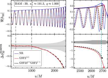
Figure 12: Phasing comparison for the case involving BNSs with spins, specifically BAM:0039 with $q=1$, $\Lambda=1001.8$ and dimensionless spins $\chi_{1}=\chi_{2}=0.14$. See the caption of Fig. 9 for details.

Appendix A Derivation of the GSF-resummed (3+) potential

We follow the formalism and notation of Ref. Bini and Damour (2014) (henceforth BD). For more details, see their work. Setting the NS label $A=1$ we have

$$\hat{A}^{(3+)}_{1} =\hat{A}_{1}^{(3+)\text{0GSF}}+\hat{A}_{1}^{(3+)\text{1GSF}}X_{1}+\hat{A}_{1}^{(3+)\text{2GSF}}X_{1}^{2}.$$ (38)

To obtain the explicit expression for $\hat{A}_{1}^{(3+)\text{1GSF}}$ we start with Eq. (6.11) of BD

$$\hat{A}^{(3+)}_{1}(u)=\sqrt{F(u;\nu)}\,\Gamma^{-1}[y(u)]\,\frac{J_{3+}[y(u)]}{J^{\text{Newt}}_{3+}(u)},$$ (39)

where $\Gamma(y)$ is the usual redshift factor and $y\equiv(m_{2}\Omega)^{2/3}$ is the GSF inverse separation. $F(u;\nu)$ is a function of the circular-orbit, “bare” potential $A(u)$ and its derivative, and $J^{\text{Newt}}_{3+}=90m_{2}^{2}/r^{8}_{\text{EOB}}$ which becomes $J^{\text{Newt}}_{3+}(u)=90X_{2}^{8}u^{8}/m_{2}^{6}$ using $r_{\text{EOB}}=M/u$. This results in

$$\hat{A}^{(3+)}_{1}(u)=\frac{\sqrt{F(u;\nu)}}{(1-X_{1})^{8}}\,\Gamma^{-1}[y(u)]\,\frac{m_{2}^{6}J_{3+}[y(u)]}{90u^{8}},$$ (40)

which is the $(3+)$ version of BD Eq. (7.3). Note that Eq. (39) is a general expression that holds for all order of $X_{1}$, but current GSF knowledge limits us to $\mathcal{O}(X_{1})$. Additionally, the $\mathcal{O}(X_{1})$ difference between the EOB inverse separation $u$ and the GSF inverse separation $y$ needs to be accounted for [cf. Eqs. (2.18, 2.19) of BD].

Combining the work of Ref. Nolan et al. (2015) and BD App. D we have that $J_{3+}=K_{3+}+\tfrac{1}{3}J_{\dot{2}+}$ where the latter are given as a series in $q\equiv X_{1}/X_{2}\ll 1$

$$K_{3+} =K_{3+}^{\text{0GSF}}\left[1+q\left(\hat{\delta}k_{3+}+2h_{uu}\right)\right],$$ (41)

$$J_{\dot{2}+} =J_{\dot{2}+}^{\text{0GSF}}\left[1+q\,\Delta j_{\dot{2}+}\right]\equiv J_{\dot{2}+}^{\text{0GSF}}\left[1+q\,(\hat{\delta}j_{\dot{2}+}+3h_{uu})\right],$$ (42)

where numerical values for $\hat{\delta}k_{3+}$ are given in Table V of Ref. Nolan et al. (2015) and $\Delta j_{\dot{2}+}$ can be obtained from Ref. Nolan et al. (2015) Eqs. (2.44, 2.45) in terms of Ref. Dolan et al. (2015)’s redshift and spin-precession invariants. $\hat{\delta}j_{\dot{2}+}$ is given as PN series in Appendix D of BD. $h_{uu}\equiv 2\Delta U/U_{0}$ where $U_{0}=(1-3y)^{-1/2}$.

The background, i.e., 0GSF terms in Eqs. (41, 42) can be extracted from Ref. Nolan et al. (2015) or Appendix D of BD. They read

$$K_{3+}^{\text{0GSF}} =6y^{8}(1-2y)\frac{(42y^{2}-46y+15)}{(1-3y)^{2}},$$ (43)

$$J_{\dot{2}+}^{\text{0GSF}} =\frac{18y^{9}(1-2y)^{2}}{(1-3y)^{2}}.$$ (44)

With the above equations and the numerical data of Refs. Dolan et al. (2015); Nolan et al. (2015) we can now calculate the 1-GSF contribution to $\hat{A}^{(3+)}$. We performed several checks on our result:

1. 0-GSF limit: Simply taking the $q\sim X_{1}\to 0$ limit of our expression for $\hat{A}^{(3+)}$ yields

   $$\hat{A}^{(3+)\text{0GSF}}=(1-2u)\left(1+\frac{8}{3}\frac{u^{2}}{(1-3u)}\right)\,.$$ (45)

   This agrees with the test-mass limit result given by Eq. (6.45) of Ref. Bini et al. (2012).

2. Weak-field limit: Using BD’s PN series expansions for $\hat{\delta}k_{3+}$ and $\hat{\delta}j_{\dot{2}+}$ and Ref. Kavanagh et al. (2015)’s series for $\Delta U$ we straightforwardly obtain the PN series for $\hat{A}^{(3+)}(u)$

   $$\lim_{u\to 0}\hat{A}^{(3+)\text{1GSF}}=\frac{15}{2}u-\frac{311}{24}u^{2}+\mathcal{O}(u^{3})\,$$ (46)

   which agrees with the $\mathcal{O}(X_{1})$ part of Eq. (13). Our numerical data is also consistent with this as can be seen in Fig. 13.

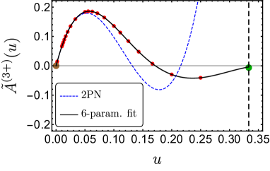
Figure 13: $\tilde{A}^{(3+)}\equiv(1-3u)^{7/2}\hat{A}^{(3+)\text{1GSF}}$ data in red dots with the PN series as the blue dashed curve. The values for the $\tilde{A}^{(3+)}(u)$ data set are obtained using the numerical data for the tidal invariants of Refs. Dolan et al. (2015); Nolan et al. (2015). The black curve is our six-parameter fit given by Eqs. (50)-(51). The green dot marks the light-ring limit and the brown dot the $u\to 0$ limit. The vertical dashed black line marks the position of the light ring.

We next investigate the light-ring (LR) limit. BD provide ample explanations on how to ascertain the singular behaviour of $\hat{A}^{(\ell\pm)}$ as $u\to 1/3$ and how to obtain the LR limit of singularity-factored potentials $\tilde{A}^{(2\pm)}\equiv(1-3u)^{7/2}\hat{A}^{(2\pm)\text{1GSF}}$. Following the same analysis, we straightforwardly establish that

$$\lim_{u\to\tfrac{1}{3}}\hat{A}^{(3+)\text{1GSF}} =-\frac{\zeta}{162}(1-3u)^{-7/2}$$

$$=\frac{8}{27}\left(-\frac{\zeta}{48}(1-3u)^{-7/2}\right),$$ (47)

where the last quantity in parentheses is the LR limit of $\hat{A}^{(2\pm)\text{1GSF}}$.

Accordingly, we now introduce the LR rescaled function

$$\tilde{A}^{(3+)}(u)\equiv(1-3u)^{7/2}\hat{A}^{(3+)\text{1GSF}}\!(u)$$ (48)

whose PN series expansion

$$\tilde{A}^{(3+)}(u\ll 1)=\frac{15}{2}u\left[1-\frac{2201}{180}u+\mathcal{O}(u^{2})\right]$$ (49)

hints a cubic strong-field fit to the data of the form $\tfrac{15}{2}u(1+C_{1}u+C_{2}u^{2})$. However, after much experimenting we settled on the following best fit to the data

$$\tilde{A}^{(3+)}(u) \approx\tilde{A}^{(3+)}_{\text{fit}}(u)$$ (50)

$$=\frac{15}{2}u(1+C_{1}u+C_{2}u^{2}+C_{3}u^{3})\,\frac{1+C_{4}u+C_{5}u^{2}}{1+C_{6}u^{2}},$$

where

$$C_{1} =-3.682095,\qquad C_{2}=\ 5.171003,$$

$$C_{3} =-7.639164,\qquad C_{4}=-8.632781,$$

$$C_{5} =16.36009,\qquad\ \ C_{6}=12.31964\,.$$ (51)

This fit and a 2PN expression for $\tilde{A}^{(3+)}$ are shown as the black and blue curves in Fig. 13, respectively. Although our fitting procedure excluded the data point at the light ring, our fit nearly crosses it anyway (see Fig. 13). Additionally, the fit approximates every one of the 23 data points to a relative difference of $<5\times 10^{-4}$ with the exception of one point with 1% mismatch and another 0.1%. The norm of the relative disagreement over the entire data is

$$||1-\tilde{A}^{(3+)}_{\text{fit}}/\tilde{A}^{(3+)\text{1SF}}_{\text{num}}||\approx 0.0118\,.$$ (52)

Putting everything together, we arrive at

$$\hat{A}_{A}^{(3+)}\,=\ (1-2u)\left(1+\frac{8}{3}\frac{u^{2}}{(1-3u)}\right)$$

$$+X_{A}\,\frac{\tilde{A}^{(3+)}_{\text{fit}}(u)}{(1-3u)^{7/2}}+X_{A}^{2}\,\frac{110}{3}\frac{u^{2}}{(1-3u)^{p_{3+}}}.$$ (53)

Appendix B Post-adiabatic dynamics

Within TEOBResumS, the dynamics of a (non-precessing) binary system is usually determined by numerically solving four of Hamilton’s equations. The time needed to solve these four ODEs is the main contribution to the waveform evaluation time. Using our publicly available C code (see main text) a typical time-domain BNS waveform requires $\sim 1$ sec to be generated starting from a GW frequency of 10 Hz and employing standard Runge-Kutta integration routines with adaptive timestep. Thus, ODE integration cannot be used in parameter estimation runs that require the generation of $~{}10^{7}$ waveforms. Ref. Nagar and Rettegno (2018) pointed out a way of reducing the evaluation time by making use of the PA approximation to compute the system dynamics. While the approach was then restricted to the inspiral phase, we here present, for the first time, results that include the full evolution up to merger.

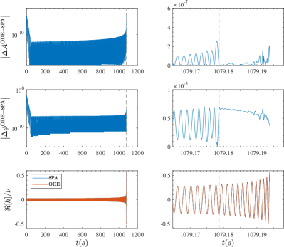
Figure 14: Comparison between the waveforms computed solving the ODEs with the GSL rk8 routine and adaptive timestep, and the PA waveform completed with the same ODE solver after $r<r_{\text{min}}$ for a non-spinning BNS system with $1.35M_{\odot}+1.35M_{\odot}$ and SLy EOS starting at $10$ Hz. The PA parameters used are the ones described in the second row of Table 4. The dashed grey line marks the stitching point, $r_{\text{min}}$, between the PA and ODE-based dynamics. Having written the waveform strain as $h/\nu\equiv Ae^{\rm-i\phi}$, we defined the phase difference as $\Delta\phi^{\rm ODE-8PA}\equiv\phi^{\rm ODE}-\phi^{\rm 8PA}$ and the fractional amplitude difference as $\Delta A^{\rm ODE-8PA}\equiv(A^{\rm ODE}-A^{\rm 8PA})/A^{\rm ODE}$. The higher differences at the start of the evolution are due to the fact that the complete ODE is currently started using only 2PA data.

We start by briefly summarizing the procedure described in Ref. Nagar and Rettegno (2018). The PA approximation is an extension of the one introduced in Refs. Buonanno and Damour (1999, 2000) (and expanded in Refs. Damour and Nagar (2008); Damour et al. (2013)) and is currently used to determine the initial conditions of TEOBResumS. Using this approximation, it is possible to analytically compute the radial and angular momentum of a binary system, under the assumption that the GW flux is small. This is obviously true in the early inspiral phase and progressively loses validity when the two objects get close. The approach starts by considering the conservative system, when the flux is null, and then computes the successive corrections to the momenta. We denote with $n$PA the $n$-th order iteration of this procedure.

$f_{0}$ [Hz]	$r_{0}$	$r_{\rm min}$	$N_{r}$	$\Delta r$	$\tau_{\rm 8PA}$ [sec]	$\tau_{\rm ODE}$ [sec]
20	112.80	12	500	0.20	0.04	0.53
10	179.01	12	800	0.21	0.06	1.26

Table 4: Performance of the TEOBResumS C code for a non-spinning BNS system with $1.35M_{\odot}+1.35M_{\odot}$ and SLy EOS. $f_{0}$ and $r_{0}$ denote the initial GW frequency and radial separation (in units of $(GM)/c^{2}$). The 8PA dynamics is computed on a grid with $N_{r}$ points and grid separation $\Delta r$ that ends at $r_{\rm min}$ and then completed by the standard ODE one. The evaluation times $\tau$ are determined using a standard Intel Core i7, 1.8GHz and 16GB RAM. The code is compiled with the GNU gcc compiler using O3 optimization.

Practically, to compute the PA dynamics, we first build a uniform radial grid from the initial radius $r_{0}$ to an $r_{\text{min}}$ up until which we are sure the approximation holds. We then analytically compute the momenta that correspond to each radius at a chosen PA order. Finally, we determine the full dynamics recovering the time and orbital phase by quadratures. From $r_{\text{min}}$ we can then start the usual ODE-based dynamics using the PA quantities as initial data as it is usually done (at 2PA order) in TEOBResumS. The benefits of using this method come from the fact that we can avoid the numerical solution of two Hamilton’s equations and that we can integrate the other two on a very sparse radial grid.

$f_{0}$ [Hz]	$r_{0}$	$\tau_{\rm 8PA}^{\rm int}$ [sec]	$\tau_{\rm ODE}^{\rm int}$ [sec]
20	112.80	0.54	1.06
10	179.01	3.2	4.4

Table 5: Performance of the TEOBResumS C code when the final waveform is interpolated on a time grid sampled at 1/(4096 Hz). We use a standard, non-optimized, GSL interpolation routine. The considered system coincides with the one of Table 4.

With the initial radius is fixed, there are three parameters that can be chosen at will in the PA procedure. These are the PA order, the number of grid points (or, equivalently, the grid step), and $r_{\rm min}$. We use the 8PA order, a grid separation $\Delta r\sim 0.2$, and $r_{\rm min}\sim 12$ (note the latter value can be tuned depending on the BNS spin).

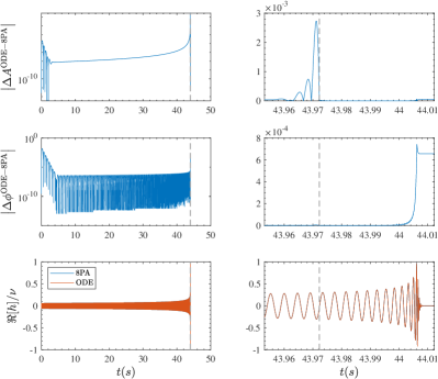
Figure 15: Comparison of Fig. 14 in a case of a BBH system with $m_{A}=m_{B}=3M_{\odot}$ and $\chi_{A}=\chi_{B}=-0.99$. The evolution is started at a GW frequency $f_{0}=20$ Hz, which corresponds to an initial radius $r_{0}=66.34$. The 8PA dynamics is computed using a grid separation $\Delta r=0.2$ and then stitched to the ODE-based one at $r_{\text{min}}=13$.

This is a conservative choice of parameters that guarantees a remarkable agreement with the dynamics computed by solving the ODEs. We show in Fig. 14 the waveform fractional-amplitude difference (top panel) and phase difference (medium panel) for a non-spinning BNS system with $1.35M_{\odot}+1.35M_{\odot}$ and SLy EOS. The vertical dashed line marks the stitching point between the PA evolution and the ODE evolution for the last orbits where the PA approximation brakes down. Table 4 highlights the performances of the C code for such a case. Here, the initial radius is determined by solving the circular Hamilton’s equations instead of relying on Kepler’s law, as discussed in Sec. VI of Ref. Nagar et al. (2018).

We can see that the waveform computed using the PA dynamics (completed with the ODE for the last few orbits) only takes around 60 milliseconds to be evaluated. Such a time is competitive with respect to the surrogate models that are currently being constructed in order to reduce waveform evaluation times Lackey et al. (2017). Finally, Table 5 illustrates the performance of TEOBResumS when the waveform, which is obtained on a nonuniform temporal grid, is interpolated on an evenly spaced time grid, sampled at $\Delta t^{-1}=4096$ Hz. Note that the interpolation routine is not optimized, and as such, it by far makes the dominant contribution to the global computational cost.

B.1 Binary black hole case

For completeness, we also show in Fig. 15 a case of a binary black hole (BBH) system, completed with the postmerger and ringdown phase. We consider an equal-mass black-hole binary with $m_{A}=m_{B}=3M_{\odot}$ and nearly extremal anti-aligned spins, $\chi_{A}=\chi_{B}=-0.99$. We do not want to discuss these cases in detail here. It suffices to note that the main conclusions do not change when we take into account BBH systems.

References

- Abbott et al. (2017) B. P. Abbott et al. (Virgo, LIGO Scientific), Phys. Rev. Lett. 119, 161101 (2017), arXiv:1710.05832 [gr-qc] .
- Abbott et al. (2018a) B. P. Abbott et al. (Virgo, LIGO Scientific), (2018a), arXiv:1805.11581 [gr-qc] .
- Abbott et al. (2018b) B. P. Abbott et al. (Virgo, LIGO Scientific), (2018b), arXiv:1805.11579 [gr-qc] .
- Baiotti et al. (2010) L. Baiotti, T. Damour, B. Giacomazzo, A. Nagar, and L. Rezzolla, Phys. Rev. Lett. 105, 261101 (2010), arXiv:1009.0521 [gr-qc] .
- Bernuzzi et al. (2012a) S. Bernuzzi, A. Nagar, M. Thierfelder, and B. Brügmann, Phys.Rev. D86, 044030 (2012a), arXiv:1205.3403 [gr-qc] .
- Bernuzzi et al. (2015) S. Bernuzzi, A. Nagar, T. Dietrich, and T. Damour, Phys.Rev.Lett. 114, 161103 (2015), arXiv:1412.4553 [gr-qc] .
- Hinderer et al. (2016) T. Hinderer et al., Phys. Rev. Lett. 116, 181101 (2016), arXiv:1602.00599 [gr-qc] .
- Buonanno and Damour (1999) A. Buonanno and T. Damour, Phys. Rev. D59, 084006 (1999), arXiv:gr-qc/9811091 .
- Buonanno and Damour (2000) A. Buonanno and T. Damour, Phys. Rev. D62, 064015 (2000), arXiv:gr-qc/0001013 .
- Damour and Nagar (2010) T. Damour and A. Nagar, Phys. Rev. D81, 084016 (2010), arXiv:0911.5041 [gr-qc] .
- Damour (1983) T. Damour, in Gravitational Radiation, edited by N. Deruelle and T. Piran (North-Holland, Amsterdam, 1983) pp. 59–144.
- Hinderer (2008) T. Hinderer, Astrophys.J. 677, 1216 (2008), arXiv:0711.2420 [astro-ph] .
- Flanagan and Hinderer (2008) E. E. Flanagan and T. Hinderer, Phys.Rev. D77, 021502 (2008), arXiv:0709.1915 [astro-ph] .
- Damour and Nagar (2009a) T. Damour and A. Nagar, Phys. Rev. D80, 084035 (2009a), arXiv:0906.0096 [gr-qc] .
- Binnington and Poisson (2009) T. Binnington and E. Poisson, Phys. Rev. D80, 084018 (2009), arXiv:0906.1366 [gr-qc] .
- Hinderer et al. (2010) T. Hinderer, B. D. Lackey, R. N. Lang, and J. S. Read, Phys. Rev. D81, 123016 (2010), arXiv:0911.3535 [astro-ph.HE] .
- Vines and Flanagan (2010) J. E. Vines and E. E. Flanagan, Phys. Rev. D88, 024046 (2010), arXiv:1009.4919 [gr-qc] .
- Vines et al. (2011) J. Vines, E. E. Flanagan, and T. Hinderer, Phys. Rev. D83, 084051 (2011), arXiv:1101.1673 [gr-qc] .
- Damour et al. (2012a) T. Damour, A. Nagar, and L. Villain, Phys.Rev. D85, 123007 (2012a), arXiv:1203.4352 [gr-qc] .
- Bini et al. (2012) D. Bini, T. Damour, and G. Faye, Phys.Rev. D85, 124034 (2012), arXiv:1202.3565 [gr-qc] .
- Bini and Damour (2014) D. Bini and T. Damour, Phys.Rev. D90, 124037 (2014), arXiv:1409.6933 [gr-qc] .
- Banihashemi and Vines (2018) B. Banihashemi and J. Vines, (2018), arXiv:1805.07266 [gr-qc] .
- Damour et al. (2009) T. Damour, B. R. Iyer, and A. Nagar, Phys. Rev. D79, 064004 (2009), arXiv:0811.2069 [gr-qc] .
- Faye et al. (2015) G. Faye, L. Blanchet, and B. R. Iyer, Class. Quant. Grav. 32, 045016 (2015), arXiv:1409.3546 [gr-qc] .
- Hotokezaka et al. (2013) K. Hotokezaka, K. Kyutoku, and M. Shibata, Phys.Rev. D87, 044001 (2013), arXiv:1301.3555 [gr-qc] .
- Bernuzzi et al. (2012b) S. Bernuzzi, M. Thierfelder, and B. Brügmann, Phys.Rev. D85, 104030 (2012b), arXiv:1109.3611 [gr-qc] .
- Dolan et al. (2015) S. R. Dolan, P. Nolan, A. C. Ottewill, N. Warburton, and B. Wardell, Phys. Rev. D91, 023009 (2015), arXiv:1406.4890 [gr-qc] .
- Damour and Nagar (2014) T. Damour and A. Nagar, Phys.Rev. D90, 044018 (2014), arXiv:1406.6913 [gr-qc] .
- Nagar et al. (2017) A. Nagar, G. Riemenschneider, and G. Pratten, Phys. Rev. D96, 084045 (2017), arXiv:1703.06814 [gr-qc] .
- Nagar et al. (2018) A. Nagar et al., (2018), arXiv:1806.01772 [gr-qc] .
- Dietrich and Hinderer (2017) T. Dietrich and T. Hinderer, Phys. Rev. D95, 124006 (2017), arXiv:1702.02053 [gr-qc] .
- Dietrich et al. (2018a) T. Dietrich, D. Radice, S. Bernuzzi, F. Zappa, A. Perego, B. Brügmann, S. V. Chaurasia, R. Dudi, W. Tichy, and M. Ujevic, (2018a), arXiv:1806.01625 [gr-qc] .
- Hotokezaka et al. (2015) K. Hotokezaka, K. Kyutoku, H. Okawa, and M. Shibata, Phys. Rev. D91, 064060 (2015), arXiv:1502.03457 [gr-qc] .
- Hotokezaka et al. (2016) K. Hotokezaka, K. Kyutoku, Y.-i. Sekiguchi, and M. Shibata, Phys. Rev. D93, 064082 (2016), arXiv:1603.01286 [gr-qc] .
- Kokkotas and Schäfer (1995) K. D. Kokkotas and G. Schäfer, Mon. Not. Roy. Astron. Soc. 275, 301 (1995), arXiv:gr-qc/9502034 [gr-qc] .
- Ho and Lai (1999) W. C. G. Ho and D. Lai, Mon. Not. Roy. Astron. Soc. 308, 153 (1999), arXiv:astro-ph/9812116 [astro-ph] .
- Steinhoff et al. (2016) J. Steinhoff, T. Hinderer, A. Buonanno, and A. Taracchini, Phys. Rev. D94, 104028 (2016), arXiv:1608.01907 [gr-qc] .
- Pan et al. (2011) Y. Pan, A. Buonanno, M. Boyle, L. T. Buchman, L. E. Kidder, et al., Phys.Rev. D84, 124052 (2011), arXiv:1106.1021 [gr-qc] .
- Pan et al. (2014a) Y. Pan, A. Buonanno, A. Taracchini, M. Boyle, L. E. Kidder, et al., Phys.Rev. D89, 061501 (2014a), arXiv:1311.2565 [gr-qc] .
- Pan et al. (2014b) Y. Pan, A. Buonanno, A. Taracchini, L. E. Kidder, A. H. Mroue, et al., Phys.Rev. D89, 084006 (2014b), arXiv:1307.6232 [gr-qc] .
- Taracchini et al. (2014) A. Taracchini, A. Buonanno, Y. Pan, T. Hinderer, M. Boyle, et al., Phys.Rev. D89, 061502 (2014), arXiv:1311.2544 [gr-qc] .
- Landry and Poisson (2015) P. Landry and E. Poisson, Phys. Rev. D91, 104026 (2015), arXiv:1504.06606 [gr-qc] .
- Dietrich et al. (2017a) T. Dietrich, S. Bernuzzi, and W. Tichy, Phys. Rev. D96, 121501 (2017a), arXiv:1706.02969 [gr-qc] .
- Dietrich et al. (2015) T. Dietrich, N. Moldenhauer, N. K. Johnson-McDaniel, S. Bernuzzi, C. M. Markakis, B. Brügmann, and W. Tichy, Phys. Rev. D92, 124007 (2015), arXiv:1507.07100 [gr-qc] .
- Dietrich et al. (2017b) T. Dietrich, M. Ujevic, W. Tichy, S. Bernuzzi, and B. Brügmann, Phys. Rev. D95, 024029 (2017b), arXiv:1607.06636 [gr-qc] .
- Nagar and Rettegno (2018) A. Nagar and P. Rettegno, (2018), arXiv:1805.03891 [gr-qc] .
- Damour (2001) T. Damour, Phys. Rev. D64, 124013 (2001), arXiv:gr-qc/0103018 .
- Damour and Nagar (2009b) T. Damour and A. Nagar, Phys. Rev. D79, 081503 (2009b), arXiv:0902.0136 [gr-qc] .
- Yagi (2014) K. Yagi, Phys. Rev. D89, 043011 (2014), arXiv:1311.0872 [gr-qc] .
- Pani et al. (2018) P. Pani, L. Gualtieri, T. Abdelsalhin, and X. Jiménez-Forteza, (2018), arXiv:1810.01094 [gr-qc] .
- Jimenez-Forteza et al. (2018) X. Jimenez-Forteza, T. Abdelsalhin, P. Pani, and L. Gualtieri, (2018), arXiv:1807.08016 [gr-qc] .
- Yagi and Yunes (2013) K. Yagi and N. Yunes, Science 341, 365 (2013), arXiv:1302.4499 [gr-qc] .
- Nolan et al. (2015) P. Nolan, C. Kavanagh, S. R. Dolan, A. C. Ottewill, N. Warburton, and B. Wardell, Phys. Rev. D92, 123008 (2015), arXiv:1505.04447 [gr-qc] .
- Damour et al. (2013) T. Damour, A. Nagar, and S. Bernuzzi, Phys.Rev. D87, 084035 (2013), arXiv:1212.4357 [gr-qc] .
- Damour and Gopakumar (2006) T. Damour and A. Gopakumar, Phys. Rev. D73, 124006 (2006), arXiv:gr-qc/0602117 .
- Bernuzzi et al. (2014) S. Bernuzzi, A. Nagar, S. Balmelli, T. Dietrich, and M. Ujevic, Phys.Rev.Lett. 112, 201101 (2014), arXiv:1402.6244 [gr-qc] .
- Dietrich et al. (2018b) T. Dietrich, S. Bernuzzi, B. Brügmann, M. Ujevic, and W. Tichy, Phys. Rev. D97, 064002 (2018b), arXiv:1712.02992 [gr-qc] .
- Bernuzzi and Dietrich (2016) S. Bernuzzi and T. Dietrich, Phys. Rev. D94, 064062 (2016), arXiv:1604.07999 [gr-qc] .
- Damour et al. (2012b) T. Damour, A. Nagar, D. Pollney, and C. Reisswig, Phys.Rev.Lett. 108, 131101 (2012b), arXiv:1110.2938 [gr-qc] .
- De et al. (2018) S. De, D. Finstad, J. M. Lattimer, D. A. Brown, E. Berger, and C. M. Biwer, (2018), arXiv:1804.08583 [astro-ph.HE] .
- Radice et al. (2018) D. Radice, A. Perego, F. Zappa, and S. Bernuzzi, Astrophys. J. 852, L29 (2018), arXiv:1711.03647 [astro-ph.HE] .
- Damour et al. (2008) T. Damour, P. Jaranowski, and G. Schäfer, Phys.Rev. D78, 024009 (2008), arXiv:0803.0915 [gr-qc] .
- Akcay et al. (2012) S. Akcay, L. Barack, T. Damour, and N. Sago, (2012), arXiv:1209.0964 [gr-qc] .
- Damour (2018) T. Damour, Phys. Rev. D97, 044038 (2018), arXiv:1710.10599 [gr-qc] .
- Nagar and Shah (2016) A. Nagar and A. Shah, Phys. Rev. D94, 104017 (2016), arXiv:1606.00207 [gr-qc] .
- Messina et al. (2018) F. Messina, A. Maldarella, and A. Nagar, Phys. Rev. D97, 084016 (2018), arXiv:1801.02366 [gr-qc] .
- Bohé et al. (2015) A. Bohé, G. Faye, S. Marsat, and E. K. Porter, Class. Quant. Grav. 32, 195010 (2015), arXiv:1501.01529 [gr-qc] .
- Pani et al. (2015a) P. Pani, L. Gualtieri, A. Maselli, and V. Ferrari, Phys. Rev. D92, 024010 (2015a), arXiv:1503.07365 [gr-qc] .
- Pani et al. (2015b) P. Pani, L. Gualtieri, and V. Ferrari, (2015b), arXiv:1509.02171 [gr-qc] .
- Landry (2017) P. Landry, Phys. Rev. D95, 124058 (2017), arXiv:1703.08168 [gr-qc] .
- Gagnon-Bischoff et al. (2018) J. Gagnon-Bischoff, S. R. Green, P. Landry, and N. Ortiz, Phys. Rev. D97, 064042 (2018), arXiv:1711.05694 [gr-qc] .
- Landry (2018) P. Landry, (2018), arXiv:1805.01882 [gr-qc] .
- Abdelsalhin et al. (2018) T. Abdelsalhin, L. Gualtieri, and P. Pani, (2018), arXiv:1805.01487 [gr-qc] .
- Lange et al. (2018) J. Lange, R. O’Shaughnessy, and M. Rizzo, (2018), arXiv:1805.10457 [gr-qc] .
- Lackey et al. (2017) B. D. Lackey, S. Bernuzzi, C. R. Galley, J. Meidam, and C. Van Den Broeck, Phys. Rev. D95, 104036 (2017), arXiv:1610.04742 [gr-qc] .
- Kawaguchi et al. (2018) K. Kawaguchi, K. Kiuchi, K. Kyutoku, Y. Sekiguchi, M. Shibata, and K. Taniguchi, Phys. Rev. D97, 044044 (2018), arXiv:1802.06518 [gr-qc] .
- Dietrich et al. (2018c) T. Dietrich et al., (2018c), arXiv:1804.02235 [gr-qc] .
- Kavanagh et al. (2015) C. Kavanagh, A. C. Ottewill, and B. Wardell, Phys. Rev. D92, 084025 (2015), arXiv:1503.02334 [gr-qc] .
- Damour and Nagar (2008) T. Damour and A. Nagar, Phys. Rev. D77, 024043 (2008), arXiv:0711.2628 [gr-qc] .