Exploring redshift-space distortions in large-scale structure

Abstract

We explore and compare different ways large-scale structure observables in redshift-space and real space can be connected. These include direct computation in Lagrangian space, moment expansions and two formulations of the streaming model. We derive for the first time a Fourier space version of the streaming model, which yields an algebraic relation between the real- and redshift-space power spectra which can be compared to earlier, phenomenological models. By considering the redshift-space 2-point function in both configuration and Fourier space, we show how to generalize the Gaussian streaming model to higher orders in a systematic and computationally tractable way. We present a closed-form solution to the Zeldovich power spectrum in redshift space and use this as a framework for exploring convergence properties of different expansion approaches. While we use the Zeldovich approximation to illustrate these results, much of the formalism and many of the relations we derive hold beyond perturbation theory, and could be used with ingredients measured from N-body simulations or in other areas requiring decomposition of Cartesian tensors times plane waves. We finish with a discussion of the redshift-space bispectrum, bias and stochasticity and terms in Lagrangian perturbation theory up to 1-loop order.

1 Introduction

The large-scale structure of the Universe contains valuable information about cosmology and fundamental physics, and a number of ambitious observational campaigns to extract this information are underway or in the planning stages [1, 2]. These new observations will provide increasingly precise measurements of the clustering of astrophysical objects on large scales, which are relatively simple to model and where predictions are under theoretical control. Much as for anisotropies in the cosmic microwave background, it is hoped that the combination of robust theoretical predictions and exquisitely sensitive observations will yield strong constraints on cosmological models (e.g. Ref. [3]).

In this paper we are interested in developing analytic models for the large scale clustering of objects in redshift space [4], i.e. as measured in galaxy redshift surveys [5, 6, 7, 2], the Ly$\alpha$ forest [8, 9] or line intensity mapping experiments [10]. In these situations the line-of-sight peculiar motions of objects contribute to their observed redshift so that they are placed at the incorrect (line-of-sight) distance [11, 12, 13, 4]. This velocity-induced mapping from real- to redshift-space introduces an anisotropy in the clustering pattern, which can be used to test the theory and probe the growth of large-scale structure [14, 15].

While many of our results will be valid in general, for explicit calculations and to better bring out the physics implied by our formulae we will use Lagrangian perturbation theory (see e.g. Ref. [16], building upon the work of Refs. [17, 18, 19, 20, 21, 22, 23, 24, 25, 26, 27, 28, 29, 30, 31]). Our focus will be on the study the low-order statistics of redshift-space fields in both configuration and Fourier space.

The outline of the paper is as follows. In §2 we review some background material on our model and establish our notation. In §3 we introduce the main results of this paper, namely a comparison of different formalims for computing the redshift-space 2-point functions. This section also includes the development of a new variant of the streaming model, which has some advantages over previous treatments. We apply the general formalism in §4 and §5, where we compare the different approaches for computing the redshift-space power spectrum and correlation function (respectively) to the direct calculation, allowing a detailed study of the convergence properties of each method. While most of the comparisons are done for the matter field within the Zeldovich approximation, our formalism is much more general and §6 explicitly develops the bias and loop expansions. We show that the moment expansion and Fourier-space version of the streaming model lead to relatively simple expressions for the 3-point function in Fourier space (i.e. the bispectrum) in §7. We conclude in §8. Some technical details are relegated to a series of appendices.

Throughout the paper, we will use the index-summation convention where possible, the subscript $L$ will denote the linear (Eulerian) quantities, and we will be assuming the $\Lambda$CDM cosmology with $\Omega_{m}=0.295$, $\Omega_{b}=0.047$, $n_{s}=0.968$, $\sigma_{8}=0.835$ and $h=0.688$.

2 Background

In this section we give a brief review of Lagrangian perturbation theory to fix our notation. We refer the reader to the references below for the development of the theory. Lagrangian perturbation theory and effective field theory, coupled with a flexbile bias model, offer a systematic and accurate means of predicting the clustering of biased tracers in both configuration and Fourier space (e.g. Ref. [16]).

The Lagrangian approach to cosmological structure formation was developed in [17, 18, 19, 20, 21, 22, 23, 24, 25, 26, 27, 28, 29, 30, 31] and traces the trajectory of an individual fluid element through space and time. A fluid element located at position $\mathbf{q}$ at some initial time $t_{0}$ moves as $\mathbf{x}(\mathbf{q},t)=\mathbf{q}+\mathbf{\Psi}(\mathbf{q},t)$ with $\ddot{\mathbf{\Psi}}+\mathcal{H}\dot{\mathbf{\Psi}}=-\nabla\Phi(\mathbf{q}+\mathbf{\Psi})$ where an overdot represents a derivative with respect to conformal time and $\mathcal{H}=aH$ is the conformal Hubble parameter. Every element of the fluid is uniquely labeled by $\mathbf{q}$ and $\mathbf{\Psi}(\mathbf{q},t)$ fully specifies the evolution. We shall solve for $\mathbf{\Psi}$ perturbatively. The first order solution, linear in the density field, is the Zeldovich approximation [17], which will play an important role in this paper. Given $\mathbf{\Psi}$, the real-space density field at any time is simply

$$1+\delta(\mathbf{x})=\int d^{3}q\ \delta_{D}\big{[}\mathbf{x}-\mathbf{q}-\mathbf{\Psi}(\mathbf{q})\big{]}\quad\Rightarrow\quad\delta(\mathbf{k})=\int d^{3}q\ e^{i\mathbf{k}\cdot\mathbf{q}}\big{(}e^{i\mathbf{k}\cdot\mathbf{\Psi}(\mathbf{q})}-1\big{)}.$$ (2.1)

The density of biased tracers can be modeled, assuming Lagrangian bias, by multiplying the $\delta_{D}$ in the above by a function, $F[\delta_{L}(\mathbf{q}),\nabla^{2}\delta_{L}(\mathbf{q}),\cdots]$, depending upon the linear theory density and its derivatives [23, 25, 16]. In the absence of explicit knowledge of $F$, the expectation values of derivatives of $F$ take the place of unknown bias coefficients describing the tracer under consideration. Evaluation of the power spectrum then involves the expectation value of an exponential, which can be evaluated using the cumulant theorem – we refer the reader to the above references for further details and explicit calculations.

In what follows we will pay particular attention to the $1^{\rm st}$ order solution to Lagrangian dynamics, i.e. the Zeldovich approximation [17]. Since the displacement field is given in terms of the linear overdensity as $\mathbf{\Psi}(\mathbf{p})=(i\mathbf{p}/p^{2})\ \delta_{L}(\mathbf{p})$ (where $\mathbf{p}$ is the momentum variable corresponding to the Lagrangian coordinate $\mathbf{q}$), it follows that the Zeldovich matter power spectrum is given by [21, 32, 33, 22, 23, 25, 34, 35]

$$P(\mathbf{k})=\int d^{3}q\ e^{i\mathbf{k}.\mathbf{q}}\exp\left[-\frac{1}{2}k_{i}k_{j}A_{ij}(\mathbf{q})\right]$$ (2.2)

with $A_{\ell m}(\mathbf{q})=\left\langle\Delta_{\ell}\Delta_{m}\right\rangle$, and $\Delta_{i}=\Psi_{i}(\mathbf{q})-\Psi_{i}(\mathbf{0})$ (see §3 and Eq. (3.8), setting $\Delta u=0$ and $\delta_{a}=\delta_{b}=0$). The argument of the exponential can be expressed in terms of integrals over the linear theory power spectrum. Writing $A_{ij}(\mathbf{q})=X(q)\delta_{ij}+Y(q)\hat{q}_{i}\hat{q}_{j}=\tfrac{2}{3}\delta^{K}_{ij}\left(\mathcal{J}_{0}(0)-\mathcal{J}_{0}(q)\right)+2\left(\hat{q}_{i}\hat{q}_{j}-\tfrac{1}{3}\right)\mathcal{J}_{2}(q)$ we have

$$\mathcal{J}_{0}(q)=\int_{0}^{\infty}\frac{dk}{2\pi^{2}}\ P_{L}(k)j_{0}(kq)\quad{\rm and}\quad\mathcal{J}_{2}(q)=\int_{0}^{\infty}\frac{dk}{2\pi^{2}}\ P_{L}(k)j_{2}(kq),$$ (2.3)

where $j_{\ell}$ are the spherical Bessel functions. We shall return to an evaluation of Eq. (2.2) in §4.

3 Redshift space

The line-of-sight component of the peculiar motion of each object or fluid element affects its measured redshift, and thus the radial distance at which it is inferred to lie using the distance-redshift (Hubble) relation [11, 12, 13, 4]. Specifically, an object with peculiar velocity $\mathbf{v}$ which truly lies at $\mathbf{x}$ will be assigned a “redshift-space position” $\mathbf{s}=\mathbf{x}+\hat{n}\,(\mathbf{v}\cdot\hat{n}/\mathcal{H})$ if $\hat{n}$ is the line of sight. In our Lagrangian formalism, the shift to redshift space is easily accomplished by adding $\hat{n}\left(\hat{n}\cdot\dot{\mathbf{\Psi}}\right)$ to $\mathbf{\Psi}$. We shall use the shorthand notation $\dot{\mathbf{\Psi}}_{\hat{n}}$ for $\hat{n}\left(\hat{n}\cdot\dot{\mathbf{\Psi}}\right)$.

The Fourier-space density contrast in redshift space is thus

$$(2\pi)^{3}\delta^{D}(\mathbf{k})+\delta_{s}(\mathbf{k}) = \int d^{3}q\ F\exp\left[i\mathbf{k}\cdot\left\{\mathbf{q}+\mathbf{\Psi}(\mathbf{q})+\dot{\mathbf{\Psi}}_{\hat{n}}(\mathbf{q})\right\}\right]$$ (3.1)

$$= \int d^{3}x\ \left[1+\delta(\mathbf{x})\right]\exp\left[i\mathbf{k}\cdot\left\{\mathbf{x}+\mathbf{u}(\mathbf{x})\right\}\right],$$ (3.2)

where we have introduced a dimensionless velocity, $\mathbf{u}$. Note that this says the Fourier transform of the shifted field differs from that of the unshifted field by a phase, $\exp[i\mathbf{k}\cdot\mathbf{u}]$, as might have been expected. By writing this expression in Lagrangian coordinates we have not needed to make the single-stream approximation, or that the mapping $\mathbf{x}\to\mathbf{x}+\mathbf{u}(\mathbf{x})$ is one-to-one. The 2-point function of the shifted fields can now be expressed in terms of a ‘moment’ generating function (see e.g. Ref. [36])

$$1+\mathcal{M}^{ab}(\mathbf{J},\mathbf{r})=\left\langle\big{[}1+\delta_{a}(\mathbf{x}_{1})\big{]}\big{[}1+\delta_{b}(\mathbf{x}_{2})\big{]}e^{i\mathbf{J}\cdot\Delta u_{ab}}\right\rangle,$$ (3.3)

where $\Delta u_{ab}=u_{b}(\mathbf{x}_{2})-u_{a}(\mathbf{x}_{1})$ and $\mathbf{r}=\mathbf{x}_{2}-\mathbf{x}_{1}$, and $a$ and $b$ are the labels of different tracers. Note that the translational invariance of the generating function, $\mathcal{M}$, is explicit, i.e. $\mathcal{M}$ depends only on $\mathbf{r}$. This can be seen clearly by expanding the exponent and noticing that after ensemble averaging each term in the sum depends only on $\mathbf{r}$.

We can Fourier transform the generating function to obtain

$$\widetilde{\mathcal{M}}^{ab}(\mathbf{J},\mathbf{k})=\frac{k^{3}}{2\pi^{2}}\int d^{3}r\ e^{i\mathbf{k}\cdot\mathbf{r}}\left\langle(1+\delta_{a}(\mathbf{x}))(1+\delta_{b}(\mathbf{x}^{\prime}))e^{i\mathbf{J}\cdot\Delta u_{ab}}\right\rangle.$$ (3.4)

where the prefactor of $k^{3}/(2\pi^{2})$ is inserted to make $\widetilde{\mathcal{M}}$ dimensionless and for later convenience. Directly from Eqs. (3.2,3.3, 3.4) we see that the generating function, $\mathcal{M}$, has a simple relation to the power spectrum,

$$\frac{k^{3}}{2\pi^{2}}P^{ab}_{s}(\mathbf{k})=\widetilde{\mathcal{M}}^{ab}(\mathbf{J}=\mathbf{k},\mathbf{k})=\frac{k^{3}}{2\pi^{2}}\int d^{3}r\ e^{i\mathbf{k}\cdot\mathbf{r}}\mathcal{M}^{ab}(\mathbf{J}=\mathbf{k},\mathbf{r})$$ (3.5)

and that this relation holds beyond perturbation theory. We note as well that the correlation function can be obtained here by one more Fourier transform

$$\xi^{ab}_{s}(\mathbf{r})=\int\frac{d^{3}k}{(2\pi)^{3}}\ e^{-i\mathbf{k}\cdot\mathbf{r}}P^{ab}_{s}(\mathbf{k}).$$ (3.6)

We point out that to obtain the correlation function we have to perform one additional transform compared to the power spectrum regardless of whether we start from $\mathcal{M}$ or $\widetilde{\mathcal{M}}$. The reason for this, of course, is that in obtaining the power spectrum $\mathbf{J}$ could be specified as the last step, while for the correlation function the sum over the modes needs to be performed after specifying $\mathbf{J}$. This observation will lead to some interesting consequences below.

We now consider several general methods for computing the 2-point statistics of these redshift-space fields, by manipulating Eq. (3.3). There has been lots of theoretical activity in the RSD literature over the past several decades, with different approaches leading to seemingly very different models and different results. We will see that the differences in all of these approaches are simply due to different levels of approximation and techniques used to obtain the constituents. In fact, all of these approaches can be categorized based on the manner in which they approach the generating function: $\mathcal{M}$

1. Direct Lagrangian approach: the moment generating function, $\mathcal{M}$, is transformed into Lagrangian coordinates and then contributions are estimated using the cumulant theorem. Examples include Refs. [22, 23, 24, 25, 30].

2. Moment expansion approach: the exponential in the generating function, $\mathcal{M}$, is expanded and the moments individually evaluated. Examples of this approach are the distribution function approach [38, 39, 40, 41, 42, 43, 44, 45] as well as the direct SPT-loop expansion [46, 47, 48, 22]. Various Eulerian EFT based approaches also fit into this class (see e.g. Refs. [49, 50, 51, 52, 53]).

3. Streaming model: the cumulant theorem is used in Eulerian space after transforming the moment generating function $\mathcal{M}$ into the cumulant generating function $\mathcal{Z}$ (defined below in Eq. 3.14). Examples include Refs. [54, 55, 56, 57, 58, 59, 60, 16, 61].

4. Fourth approach, widely developed in the literature, is the ‘smoothing kernel’ approach. Here the cumulant expansion is used on each of the 4 contributions that arise upon expanding the product of $(1+\delta)$ terms and the exponential in Eq. (3.3), giving a result widened by a “smoothing kernel”. This approach was first presented in Ref. [36] and further developed in Ref. [37], which further expands the exponential contributions and approximates the smoothing kernel as a one parameter Fourier space Gaussian or Lorentzian.

As mentioned above, the differentiation into four classes and the labels are primarily historical. It is important to stress that all these methods would be mathematically identical if carried to the same order and with the same approximations. The differences are thus primarily of convenience: some aspects of the problem are easier to handle in some approaches than others. It is also the case that the ingredients to each method can be supplied by a perturbative, analytic model or they could (in principle) be measured in simulations. We now consider each method in turn.

3.1 Direct Lagrangian approach

Directly from the definition of $\mathbf{u}$, and using the continuity equation, we can write

$$1+\mathcal{M}^{ab}\big{(}\mathbf{J},\mathbf{r}\big{)}=\int\frac{d^{3}p}{(2\pi)^{3}}\,d^{3}q\ e^{-i\mathbf{p}\cdot(\mathbf{r}-\mathbf{q})}\ \left\langle\big{(}1+\delta_{a}\big{(}\mathbf{q}_{1}))\big{(}1+\delta_{b}(\mathbf{q}_{2})\big{)}e^{i\mathbf{p}\cdot\Delta(\mathbf{q})+i\mathbf{J}\cdot\Delta u_{ab}}\right\rangle,$$ (3.7)

and similarly

$$(2\pi)^{3}\delta^{D}(\mathbf{k})+P^{ab}_{s}(\mathbf{k})=\int d^{3}q\ e^{i\mathbf{k}\cdot\mathbf{q}}\ \left\langle\big{(}1+\delta_{a}(\mathbf{q}_{2})\big{)}\big{(}1+\delta_{b}(\mathbf{q}_{1})\big{)}\exp\Big{[}i\mathbf{k}\cdot\Delta+i\mathbf{k}\cdot\Delta u_{ab}\Big{]}\right\rangle,$$ (3.8)

where $\Delta(\mathbf{q})=\mathbf{\Psi}(\mathbf{q}_{2})-\mathbf{\Psi}(\mathbf{q}_{1})$ and all quantities are functions of Lagrangian coordinates. For the velocity in particular we have $\mathbf{u}(\mathbf{x})=\dot{\mathbf{\Psi}}_{\hat{n}}(\mathbf{q})$ for properly normalized time units. As before the redshift-space power spectrum, $P^{ab}_{s}(\mathbf{k})$, is simply the Fourier transform of $\mathcal{M}^{ab}(\mathbf{J}=\mathbf{k},\mathbf{r})$, but now expressed entirely in Lagrangian coordinates. We also note that there is no difference between using $\mathcal{M}$ or $\widetilde{\mathcal{M}}$ as the starting point for the derivation.

There has been significant attention paid to this Lagrangian framework in recent years [22, 23, 24, 25, 26, 27, 28, 29, 30, 31, 16], as it lends itself naturally to the implementation of redshift-space distortions. In addition it has been employed as the basis of an effective field theory expansion [26, 30, 16] and to model higher order correlation functions [35]. We shall consider the evaluation of this expression further later, and for now turn to the second expansion.

3.2 Moment expansion approach

The moment expansion approach is equivalent to the distribution function approach [38, 42] and proceeds by expanding the exponential term in $\mathcal{M}$ to obtain the (density weighted) moments of the velocity field (for the explicit connection to the distribution function approach we refer the reader to App A):

$$\Xi_{i_{1},\ldots,i_{n}}(\mathbf{r})=\left\langle\big{(}1+\delta_{a}(\mathbf{x})\big{)}\big{(}1+\delta_{b}(\mathbf{x}^{\prime})\big{)}\Delta u_{ab,i_{1}}\ldots\Delta u_{ab,i_{n}}\right\rangle.$$ (3.9)

We can write the power spectrum as the sum of the Fourier transforms of these moments, viz

$$(2\pi)^{3}\delta^{D}(\mathbf{k})+P^{ab}_{s}(\mathbf{k}) = \sum_{n=0}^{\infty}\frac{i^{n}}{n!}k_{i_{1}}\ldots k_{i_{n}}\widetilde{\Xi}_{i_{1},\ldots,i_{n}}(\mathbf{k})$$ (3.10)

$$= \sum_{n=0}^{\infty}\frac{i^{n}}{n!}k_{i_{1}}\ldots k_{i_{n}}\int d^{3}r\ \Xi_{i_{1},\ldots,i_{n}}(\mathbf{r})e^{i\mathbf{k}\cdot\mathbf{r}},$$ (3.11)

where $\widehat{\Xi}_{i_{1}\ldots i_{n}}^{(n)}(\mathbf{k})=(-i)^{n}\left.\partial\widetilde{\mathcal{M}}^{ab}(\mathbf{J},\mathbf{k})/\partial J_{i_{1}}\ldots\partial J_{i_{n}}\right|_{\mathbf{J}=0}$ with $\widehat{\Xi}\equiv k^{3}\widetilde{\Xi}/(2\pi^{2})$. The moment expansion approach is the most straightforward of the 3 methods, although some of the effects that can be captured nonlinearly in other approaches (e.g. finger-of-god terms in the case of RSD) might be missed here if one truncates the expansion at low order. On the other hand, such nonlinear terms should always be resummable afterwards to obtain results equivalent to the other methods. This was the strategy adopted in the distribution function approach [38, 42].

The leading order results are straightforwardly obtained within this approach. Since $u$ is a quantity of order $\delta$, we can compute the low order contributions as

$$P^{ab}_{s}(\mathbf{k}) = \widetilde{\Xi}_{0}(\mathbf{k})+ik_{i}\widetilde{\Xi}_{1,i}(\mathbf{k})-\frac{1}{2}k_{i}k_{j}\widetilde{\Xi}_{2,ij}(\mathbf{k})+\cdots$$ (3.13)

$$= \int d^{3}r\ e^{i\mathbf{k}\cdot\mathbf{r}}\left\langle\delta_{a}(\mathbf{x})\delta_{b}(\mathbf{x}^{\prime})\right\rangle$$

$$+ik_{i}\int d^{3}r\ e^{i\mathbf{k}\cdot\mathbf{r}}\Big{(}\left\langle\delta_{a}(\mathbf{x})u_{b,i}(\mathbf{x}^{\prime})\right\rangle-\left\langle\delta_{b}(\mathbf{x}^{\prime})u_{a,i}(\mathbf{x})\right\rangle\Big{)}$$

$$+k_{i}k_{j}\int d^{3}r\ e^{i\mathbf{k}\cdot\mathbf{r}}\left\langle u_{a,i}(\mathbf{x})u_{b,j}(\mathbf{x}^{\prime})\right\rangle+\cdots$$

where we have dropped terms proportional to $\delta^{D}(\mathbf{k})$. This leads to the well known Kaiser formula [11].

3.3 Streaming approach

The streaming approach is sometimes regarded as a phenomenological model, but in fact can be derived as an expansion of $\mathcal{M}$ or $\widetilde{\mathcal{M}}$ using the cumulant theorem (see below). This can be done in either configuration or Fourier space. The two forms are not equivalent, because at any finite order the cumulant expansion and the Fourier transform do not commute. The configuration space streaming model has been extensively explored in the literature [54, 55, 56, 58, 59, 60, 16] and applied to data [57, 62, 63, 64, 65]. The Fourier space expansion has not been explored in the literature to date and is new to this paper. As we will see, it has some nice properties compared to the more common, configuration-space approach, but also some subtleties.

3.3.1 Configuration space

We can perform the cumulant expansion by taking the logarithm $\mathcal{Z}^{ab}(\mathbf{J},\mathbf{r})=\ln\big{[}1+\mathcal{M}^{ab}\big{(}\mathbf{J},\mathbf{r}\big{)}\big{]}$ and expanding in $\mathbf{J}$:

$$\mathcal{Z}^{ab}(\mathbf{J},\mathbf{r})=\sum_{n=0}^{\infty}\frac{i^{n}}{n!}J_{i_{1}}\ldots J_{i_{n}}\mathcal{C}_{i_{1}\ldots i_{n}}^{(n)}(\mathbf{r}),$$ (3.14)

where $\mathcal{C}_{i_{1}\ldots i_{n}}^{(n)}(\mathbf{r})=(-i)^{n}\left.\partial\mathcal{Z}^{ab}(\mathbf{J},\mathbf{r})/\partial J_{i_{1}}\ldots\partial J_{i_{n}}\right|_{\mathbf{J}=0}$ are the cumulants of the (density weighted) velocities, $\Delta u$. The first few cumulants are

$$\mathcal{C}^{(0)}(\mathbf{r}) = \ln\big{[}1+\xi_{ab}(\mathbf{r})\big{]},$$

$$\mathcal{C}^{(1)}_{i}(\mathbf{r}) = \Xi_{i}(\mathbf{r})/\left(1+\xi_{ab}(\mathbf{r})\right),$$

$$\mathcal{C}^{(2)}_{ij}(\mathbf{r}) = \Xi_{ij}(\mathbf{r})/\left(1+\xi_{ab}(\mathbf{r})\right)-\mathcal{C}^{(1)}_{i}\mathcal{C}^{(1)}_{j},$$

$$\mathcal{C}^{(3)}_{ijk}(\mathbf{r}) = \Xi_{ijk}(\mathbf{r})/\left(1+\xi_{ab}(\mathbf{r})\right)-\mathcal{C}^{(2)}_{\{ij}\mathcal{C}^{(1)}_{k\}}-\mathcal{C}^{(1)}_{i}\mathcal{C}^{(1)}_{j}\mathcal{C}^{(1)}_{k},$$ (3.15)

where $\Xi$’s are the shift field moments given by Eq. (3.9) and the $\{\cdots\}$ indicates all the nontrivial permutations of the indices. Note that physically the denominators in the above are positive definite, however this is not guaranteed for all perturbation theory schemes and scales. The first and second cumulants are the pairwise velocity, $v_{12}$, and the dispersion, $\sigma_{12}$.

If we introduce the kernel, $\mathcal{K}^{ab}$, defined as

$$\ln\mathcal{K}^{ab}(\mathbf{k},\mathbf{r})=\sum_{n=1}^{\infty}\frac{i^{n}}{n!}k_{i_{1}}\ldots k_{i_{n}}\mathcal{C}^{(n)}_{i_{1}\ldots i_{n}}(\mathbf{r})$$ (3.16)

we can write

$$(2\pi)^{3}\delta^{D}(\mathbf{k})+P^{ab}_{s}(\mathbf{k})=\int d^{3}r\ e^{i\mathbf{k}\cdot\mathbf{r}}\big{[}1+\xi^{ab}(\mathbf{r})\big{]}\mathcal{K}^{ab}(\mathbf{k},\mathbf{r})$$ (3.17)

and

$$1+\xi^{ab}_{s}(\mathbf{s})=\int d^{3}r\ \big{[}1+\xi^{ab}(\mathbf{r})\big{]}\int\frac{d^{3}k}{(2\pi)^{3}}\ e^{-i\mathbf{k}\cdot(\mathbf{s}-\mathbf{r})}\mathcal{K}^{ab}(\mathbf{k},\mathbf{r}).$$ (3.18)

The Gaussian streaming model follows immediately by truncating the cumulant expansion in $\mathcal{K}^{ab}$ at second order,

$$1+\xi^{ab}_{s}(\mathbf{s})\simeq\int d^{3}r\ \big{[}1+\xi^{ab}(\mathbf{r})\big{]}\int\frac{d^{3}k}{(2\pi)^{3}}\ e^{-ik_{j}(s_{j}-r_{j}-\mathcal{C}^{(1)}_{j})}e^{-(1/2)k_{i}k_{j}\mathcal{C}^{(2)}_{ij}}\quad,$$ (3.19)

and doing the Gaussian integral over $d^{3}k$:

$$1+\xi^{ab}_{s}(\mathbf{s})=\int\frac{d^{3}r}{\sqrt{(2\pi)^{3}\det[\mathcal{C}^{(2)}]}}\ \big{[}1+\xi^{ab}(\mathbf{r})\big{]}\ \exp\left[-\frac{1}{2}(\mathbf{s}-\mathbf{r}-\mathcal{C}^{(1)})[\mathcal{C}^{(2)}]^{-1}(\mathbf{s}-\mathbf{r}-\mathcal{C}^{(1)})\right]\quad.$$ (3.20)

This expression can be further simplified due to the simple matrix structure of $\mathcal{C}^{(2)}$ (see later).

3.3.2 Fourier space

We can also work in Fourier space and perform the cumulant expansion by writing $\widetilde{\mathcal{Z}}^{ab}(\mathbf{J},\mathbf{k})=\ln\big{[}1+\widetilde{\mathcal{M}}^{ab}(\mathbf{J},\mathbf{k})\big{]}$ and expanding in $\mathbf{J}$ as above. The first few cumulants are

$$\widetilde{\mathcal{C}}^{(0)}(\mathbf{k}) = \ln\big{[}1+\Delta^{2}_{ab}(k)\big{]},$$ (3.21)

$$\widetilde{\mathcal{C}}^{(1)}_{i}(\mathbf{k}) = \widehat{\Xi}_{i}(\mathbf{k})/\big{[}1+\Delta^{2}_{ab}\big{]},$$

$$\widetilde{\mathcal{C}}^{(2)}_{ij}(\mathbf{k}) = \widehat{\Xi}_{ij}(\mathbf{k})/\big{[}1+\Delta^{2}_{ab}\big{]}-\widetilde{C}^{(1)}_{i}\widetilde{C}^{(1)}_{j},$$

$$\widetilde{\mathcal{C}}^{(3)}_{ijk}(\mathbf{k}) = \widehat{\Xi}_{ijk}(\mathbf{k})/\big{[}1+\Delta^{2}_{ab}\big{]}-\widetilde{C}^{(2)}_{\{ij}\widetilde{C}^{(1)}_{k\}}-\widetilde{C}^{(1)}_{i}\widetilde{C}^{(1)}_{j}\widetilde{C}^{(1)}_{k}.$$

where we have used the common notation $\Delta^{2}=k^{3}P(k)/(2\pi^{2})$ and defined $\widehat{\Xi}=k^{3}\widetilde{\Xi}/(2\pi^{2})$ as before. Since the power spectrum is always a positive quantity, both the ratios and the $\log$ in the first cumulant are well defined for all $\mathbf{k}$ and we shall assume that this property is satisfied on the relevant scales by the perturbation theories of relevance here. In analogy to what we had before, we can introduce the kernel

$$\ln\widetilde{\mathcal{K}}^{ab}(\mathbf{k})=\sum_{n=1}^{\infty}\frac{i^{n}}{n!}k_{i_{1}}\ldots k_{i_{n}}\widetilde{\mathcal{C}}^{(n)}_{i_{1}\ldots i_{n}}(\mathbf{k}).$$ (3.22)

We note that the translation kernel in this case depends on $\mathbf{k}$ only and not on $\mathbf{r}$ as was the case above. This is significant since in order to compute the power spectrum no additional Fourier transform is needed. It should be clear that the kernel $\widetilde{\mathcal{K}}^{ab}$ is not simply the Fourier transform of $\mathcal{K}^{ab}$, and neither do $\widetilde{\mathcal{Z}}^{ab}$ and $\mathcal{Z}^{ab}$ form a Fourier transform pair.

The redshift-space power spectrum can now be written

$$\frac{k^{3}}{2\pi^{2}}P^{ab}_{s}(\mathbf{k}) =\exp\left[\widetilde{\mathcal{Z}}^{ab}(\mathbf{k},\mathbf{k})\right]-1$$

$$=\big{[}1+\Delta^{2}_{ab}\big{]}\widetilde{\mathcal{K}}^{ab}(\mathbf{k})-1$$

$$=\big{[}1+\Delta^{2}_{ab}\big{]}\exp\Bigg{[}\sum_{n=1}^{\infty}\frac{i^{n}}{n!}k_{i_{1}}\ldots k_{i_{n}}\widetilde{\mathcal{C}}^{(n)}_{i_{1}\ldots i_{n}}(\mathbf{k})\Bigg{]}-1.$$ (3.23)

We note again that if we had expanded the moment generating function, $\mathcal{M}$, then the Fourier and configuration space expressions would have been conjugate. However the non-linearity inherent in the cumulant expansion (the fact that we are expanding the log of $\mathcal{M}$ and not $\mathcal{M}$ itself) means that these two “streaming models” make different predictions for both $\xi$ and $P$.

Interestingly, the configuration-space streaming model has a long history (dating back to [54, 55]), but its Fourier counterpart does not seem to have been developed previously even though it yields a much simpler power spectrum structure (Eq. 3.23).

3.4 Smoothing kernel approach

The final approach uses the cumulant expansion on each of the four terms after expanding the $(1+\delta_{a})(1+\delta_{b})$ piece of the generating function $\mathcal{M}$ in Eq. (3.3). In the case of RSD this approach was first proposed in Ref. [36] and later further developed in Ref. [37], who expanded the exponential and approximated the smoothing kernel as a Gaussian.

We re-derive this approach here in a slightly different way than presented in Ref. [36]. For details of the standard derivation we refer the reader to the original reference. We can consider writing the generating function using an ‘inertia’ operator $\hat{\mathcal{O}}=1-i\left(\partial_{\lambda_{a}}+\partial_{\lambda_{b}}\right)-\partial_{\lambda_{a}}\partial_{\lambda_{b}}$, which gives

$$1+\mathcal{M}^{ab}\big{(}\mathbf{J},\mathbf{r}\big{)}=\hat{\mathcal{O}}\left\langle e^{i\lambda_{a}\delta_{a}(\mathbf{x}_{1})+i\lambda_{b}\delta_{b}(\mathbf{x}_{2})+i\mathbf{J}\cdot\Delta u_{ab}}\right\rangle\Big{|}_{\lambda_{a}=\lambda_{b}=0}.$$ (3.24)

Defining the auxiliary quantities

$$\mathcal{A}_{ab}(\mathbf{J},\mathbf{x}_{1},\mathbf{x}_{2}) \equiv \mathbf{J}\cdot\Delta u_{ab},$$

$$\mathcal{B}_{ab}(\mathbf{J},\mathbf{x}_{1},\mathbf{x}_{2}) \equiv \mathcal{A}_{ab}(\mathbf{J},\mathbf{x}_{1},\mathbf{x}_{2})+\lambda_{a}\delta_{a}(\mathbf{x}_{1})+\lambda_{b}\delta_{b}(\mathbf{x}_{2}),$$ (3.25)

we can use the cumulant theorem to compute

$$\hat{\mathcal{O}}\left\langle e^{\mathcal{B}_{ab}}\right\rangle\bigg{|}_{\lambda_{a}=\lambda_{b}=0} = \hat{\mathcal{O}}\exp\Bigg{[}\sum_{n=2}^{\infty}\frac{i^{n}}{n!}\left\langle\mathcal{B}_{ab}^{n}\right\rangle_{c}\Bigg{]}\Bigg{|}_{\lambda_{a}=\lambda_{b}=0}$$ (3.27)

$$= \exp\Bigg{[}\sum_{n=2}^{\infty}\frac{i^{n}}{n!}\left\langle\mathcal{A}_{ab}^{n}\right\rangle_{c}\Bigg{]}\Bigg{(}1-i\sum_{n=2}^{\infty}\frac{i^{n}}{n!}\Big{(}\left\langle\partial_{a}\mathcal{B}_{ab}^{n}\right\rangle_{c}+\left\langle\partial_{b}\mathcal{B}_{ab}^{n}\right\rangle_{c}\Big{)}$$

$$-\left(\sum_{n=2}^{\infty}\frac{i^{n}}{n!}\left\langle\partial_{a}\mathcal{B}_{ab}^{n}\right\rangle_{c}\right)\left(\sum_{n=2}^{\infty}\frac{i^{n}}{n!}\left\langle\partial_{b}\mathcal{B}_{ab}^{n}\right\rangle_{c}\right)-\sum_{n=2}^{\infty}\frac{i^{n}}{n!}\left\langle\partial_{a}\partial_{b}\mathcal{B}_{ab}^{n}\right\rangle_{c}\Bigg{)}\Bigg{|}_{\lambda_{a}=\lambda_{b}=0}.$$

The generating function then becomes

$$1+\mathcal{M}^{ab}\big{(}\mathbf{J},\mathbf{r}\big{)} =\exp\Bigg{[}\sum_{n=2}^{\infty}\frac{i^{n}}{n!}\left\langle\mathcal{A}_{ab}^{n}\right\rangle_{c}\Bigg{]}\bigg{(}1+\sum_{n=1}^{\infty}\frac{i^{n}}{n!}\Big{(}\left\langle\delta_{a}\mathcal{A}_{ab}^{n}\right\rangle_{c}+\left\langle\delta_{b}\mathcal{A}_{ab}^{n}\right\rangle_{c}\Big{)}$$

$$\hskip 31.2982pt+\left(\sum_{n=1}^{\infty}\frac{i^{n}}{n!}\left\langle\delta_{a}\mathcal{A}_{ab}^{n}\right\rangle_{c}\right)\left(\sum_{n=1}^{\infty}\frac{i^{n}}{n!}\left\langle\delta_{b}\mathcal{A}_{ab}^{n}\right\rangle_{c}\right)+\sum_{n=0}^{\infty}\frac{i^{n}}{n!}\left\langle\delta_{a}\delta_{b}\mathcal{A}_{ab}^{n}\right\rangle_{c}\bigg{)}.$$ (3.28)

This can be simplified by defining a “smoothing” kernel

$$K\left(\mathbf{J},\mathbf{r}\right) \equiv \exp\Big{[}\left\langle e^{i\mathbf{J}\cdot\Delta u_{ab}}\right\rangle_{c}-1\Big{]}$$ (3.29)

$$= \exp\Bigg{[}\sum_{n=2}^{\infty}\frac{i^{n}}{n!}J_{i_{1}}\ldots J_{i_{n}}\left\langle\Delta u_{ab,i_{1}}\ldots\Delta u_{ab,i_{n}}\right\rangle_{c}\Bigg{]}.$$

This “smoothing” kernel can be considered as a general and full form of what is typically called the “finger of god” term in many RSD models. Historically this term was approximated to be a scale independent contribution, originating from the zero-lag velocity dispersion [70, 71, 72, 73, 13, 74, 75, 37]. In the literature, such terms were frequently re-summed, more often than not on phenomenological grounds, yielding the family of so-called dispersion RSD models. A serious drawback of such schemes in PT calculations was that at a certain order in PT they typically broke the Galilean invariance of the theory (see also the related discussion in e.g. [36, 41]). Note that this is explicitly not the case for the full smoothing kernel in Eq. (3.29) where, in addition to explicit Galilean invariance, the full scale dependence of the Eulerian velocity field $\Delta u$ cumulants is included in the exponent.

Finally, collecting all above, we have for the generating function

$$1+\mathcal{M}^{ab}\big{(}\mathbf{J},\mathbf{r}\big{)} =K\left(\mathbf{J},\mathbf{r}\right)\bigg{(}1+\left\langle\left(\delta_{a}+\delta_{b}\right)e^{i\mathbf{J}\cdot\Delta u_{ab}}\right\rangle_{c}$$

$$\hskip 76.82234pt+\left\langle\delta_{a}e^{i\mathbf{J}\cdot\Delta u_{ab}}\right\rangle_{c}\left\langle\delta_{b}e^{i\mathbf{J}\cdot\Delta u_{ab}}\right\rangle_{c}+\left\langle\delta_{a}\delta_{b}e^{i\mathbf{J}\cdot\Delta u_{ab}}\right\rangle_{c}\bigg{)},$$ (3.30)

where the power spectrum can now be obtained via Eq. (3.5). This result is equivalent to Eq. (31) in Ref. [36].

Note that the last step, computing the power spectrum, involves computing one additional Fourier transform. In this respect this method resembles the configuration space streaming model. However, the kernel method does not allow for a Fourier counterpart, such as in the streaming model case, and so the last integration step in Eq. (3.5) is unavoidable. Further, the quantities which enter above are most naturally evaluated in the Eulerian picture, given that the “smoothing” kernel $K(\mathbf{J},\mathbf{r})$ depends on the Eulerian velocity field $u$. Unlike in other approaches discussed earlier, $u$ is now a volume-weighted quantity rather than mass-weighted. For this reason, it is less straightforward to evaluate these correlators using Lagrangian theory, and we shall not consider this approach further in the rest of the paper. Nonetheless, it would be interesting to perform a detailed comparative study including this approach, and we hope that this question will be addressed in the future.

4 Fourier space application and comparison of methods

We now compare the performance and convergence of the different approaches detailed in the previous section, first in Fourier space (this section) and then in configuration space (§5). In order to bring out the essential points we shall adopt a simplified dynamical model, since it serves to highlight some of the more interesting aspects of the problem.

Thus, while in reality the effects of translations and nonlinear dynamics are intertwined and can give raise to effects of comparable importance on scales of interest, we shall assume they can be separated. In order to focus attention on the effects of translations, below we will restrict the dynamics to the linear displacements (i.e. the Zeldovich approximation [17]), and neglect the higher order corrections. We will also neglect bias for now. Of course this is purely for the purposes of presentation – each formalism can easily be applied to more general dynamical models and biased tracers (see §6).

Moving into redshift space amounts to replacing the displacement, $\mathbf{\Psi}$, by

$$\mathbf{\Psi}\to\mathbf{\Psi}^{s}=\mathbf{\Psi}+\frac{\hat{n}\,(\dot{\mathbf{\Psi}}\cdot\hat{n})}{\mathcal{H}}=\mathbf{R}\mathbf{\Psi}$$ (4.1)

where $R_{ij}=\delta_{ij}+f\hat{n}_{i}\hat{n}_{j}$ and $\hat{n}$ is the line of sight. In the distant-observer limit the angular dependence is normally expanded in a Legendre series:

$$P(k,\nu)=\sum_{\ell=0}^{\infty}P_{\ell}(k)\mathcal{L}_{\ell}(\nu)\quad{\rm and}\quad\xi(s,\mu_{s})=\sum_{\ell=0}^{\infty}\xi_{\ell}(s)\mathcal{L}_{\ell}(\mu_{s})$$ (4.2)

where $\mathcal{L}_{\ell}$ is the Legendre polynomial of order $\ell$, $\nu=\hat{k}\cdot\hat{n}$ and $\mu_{s}=\hat{s}\cdot\hat{n}$. Note we have used $\nu$ for what is commonly called $\mu_{k}$ to distinguish it from the other cosines which appear later. The multipole moments of $\xi$ and $P$ are related through a Hankel transform,

$$\xi_{\ell}(s)=i^{\ell}\int_{0}^{\infty}\frac{k^{2}\,dk}{2\pi^{2}}\ P_{\ell}(k)j_{\ell}(ks)$$ (4.3)

where $j_{\ell}$ is the spherical Bessel function of order $\ell$.

The linear theory predictions are the same in each approach and amount to the well known [11]

$$P_{s}(k,\nu)=\left(1+f\nu^{2}\right)^{2}P_{L}(k)\quad,$$ (4.4)

where $f$ is the growth rate $f=d\ln D/d\ln a$. In linear theory only $P_{0}$, $P_{2}$ and $P_{4}$ are non-zero and each is proportional to $P_{L}$. Including the higher order terms in the Zeldovich approximation we begin to see the differences in the approaches.

4.1 Direct Lagrangian approach

We consider two different methods to directly evaluate the Zeldovich power spectrum in redshift space. We will label the methods MI and MII. Both methods rely on representing the power spectrum in term of a series of spherical Bessel functions that can be truncated and efficiently evaluated numerically. We will compare the two methods and their efficiency.

The redshift-space power spectrum is given by Eq. (2.2) but with the transformation $A_{ij}\to A^{s}_{ij}=R_{i\ell}R_{jm}A_{\ell m}$. Note that

$$k_{i}k_{j}R_{i\ell}R_{jm}A_{\ell m} =k^{2}X\left[1+2f\nu^{2}+f^{2}\nu^{2}\right]+k^{2}Y\left[\mu^{2}+2f\mu\nu(\hat{n}\cdot\hat{q})+f^{2}\nu^{2}(\hat{n}\cdot\hat{q})^{2}\right]$$ (4.5)

$$=k^{2}X\alpha_{0}(\nu)+k^{2}Y\Big{(}\alpha_{1}(\nu)+\alpha_{2}(\nu)\gamma(\mu,\nu)\cos\phi+\alpha_{3}(\nu)\gamma(\mu,\nu)^{2}(\cos\phi)^{2}\Big{)}\mu^{2},$$

where $\mu=\hat{q}\cdot\hat{k}$, $X$ and $Y$ are linear theory displacement contributions explicitly defined in Eq. (C.2) and (C.3), and we introduce angle factors $\gamma(\mu,\nu)=\sqrt{1-\mu^{2}}\sqrt{1-\nu^{2}}/\mu\nu$ and

$$\alpha_{0}(\nu)=\Big{(}1+f\left(2+f\right)\nu^{2}\Big{)},~{}~{}~{}\alpha_{1}(\nu)=\Big{(}1+f\nu^{2}\Big{)}^{2},~{}~{}~{}\alpha_{2}(\nu)=2f\nu^{2}(1+f\nu^{2}),~{}~{}~{}\alpha_{3}(\nu)=f^{2}\nu^{4}.$$

For method MI we first perform the integral over azimuthal angle $\phi$, and thus we can write the power spectrum in the form

$$(2\pi)^{3}\delta^{D}(\mathbf{k})+P_{s}(\mathbf{k},\tau) =\int d^{3}q~{}e^{i\mathbf{k}\cdot\mathbf{q}}~{}\exp\Big{[}-\frac{1}{2}k_{i}k_{j}A^{s}_{ij}\Big{]}$$ (4.6)

$$=\int d^{3}q~{}e^{i\mathbf{k}\cdot\mathbf{q}}~{}e^{-\frac{1}{2}k^{2}\big{(}\alpha_{0}(\nu)X^{\rm lin}(q)+\alpha_{1}(\nu)\mu^{2}Y^{\rm lin}(q)\big{)}}I_{\phi}\left(\mu,\nu,-\tfrac{1}{2}k^{2}Y^{\rm lin}(q)\right).$$

where in the second line we have introduced an azimuthal integral $I_{\phi}$. We can expand $I_{\phi}$ in powers of $\mu$ to get

$$I_{\phi}\left(\mu,\nu,C\right)=\int_{0}^{2\pi}\frac{d\phi}{2\pi}~{}e^{C\mu^{2}\big{(}\alpha_{2}(\nu)\gamma(\mu,\nu)\cos(\phi)+\alpha_{3}(\nu)\gamma(\mu,\nu)^{2}\cos(\phi)^{2}\big{)}}=\sum_{\ell=0}^{\infty}F_{\ell}(\nu,\alpha_{1}C)\left(\mu^{2}\alpha_{1}C\right)^{\ell}~{},$$

where, using the confluent hypergeometric function of the first kind (Kummer’s) $M(a,b,z)$, we introduce a further function

$$F_{\ell}(\nu,x) =\sum_{m=0}^{\ell}\frac{(-1)^{m}4^{\ell-m}\Gamma(m+\tfrac{1}{2})}{\pi^{1/2}\Gamma(m+1)\Gamma(1+2m-\ell)\Gamma(2\ell-2m+1)}\left(\frac{\alpha_{0}}{\alpha_{1}}\right)^{m}$$

$$\hskip 68.28644pt\times M\left(\ell-2m;\ell-m+\tfrac{1}{2};x\right)M\left(m+\tfrac{1}{2};m+1;\frac{\alpha_{0}}{\alpha_{1}}\,x\right).$$ (4.7)

Next we do the integral over the angle $\mu$. This can be done by using well-known formulae for the integrals of powers of $\mu$ times a Gaussian in $\mu$. Following Ref. [29] and using the integral

$$\frac{1}{2}\int_{-1}^{1}d\mu~{}\mu^{2\ell}e^{i\mu A+\mu^{2}B}=\frac{(-1)^{\ell}e^{B}}{B^{\ell}}\sum_{n=0}^{\infty}U(-\ell,n-\ell+1,-B)\left(-\frac{2B}{A}\right)^{n}j_{n}(A)~{},$$ (4.8)

where $U(a,b,z)$ is a confluent hypergeometric function of the second kind (Tricomi’s), we can write the redshift-space, Zeldovich power spectrum as

$$P_{s}(k,\nu) =4\pi\sum_{n=0}^{\infty}\int q^{2}\,dq\ \mathcal{K}^{s}_{n}\big{(}k,q,\nu\big{)}\ e^{-\frac{1}{2}k^{2}\big{(}X(q)+Y(q)\big{)}}\left(\frac{k\,Y(q)}{q}\right)^{n}\,j_{n}(kq)\quad.$$ (4.9)

All of the RSD effects are contained in the kernel

$$\mathcal{K}_{n}^{s}\big{(}k,q,\nu\big{)}=\Big{(}1+f\nu^{2}\Big{)}^{2n}e^{-(1/2)f\nu^{2}k^{2}\big{[}\left(2+f\right)X(q)+\left(2+f\nu^{2}\right)Y(q)\big{]}}K^{s}_{n}\Big{(}\nu,-\tfrac{1}{2}a_{1}k^{2}Y\Big{)}$$ (4.10)

with

$$K_{n}^{s}(\nu,x) =\sum_{\ell=0}^{\infty}(-1)^{\ell}F_{\ell}(\nu,x)U(-\ell,n-\ell+1,-x).$$ (4.11)

Again, above we use standard functions $M(a,b,z)$ and $U(a,b,z)$, which are confluent hypergeometric function of the first (Kummer’s) and second (Tricomi’s) kind respectively.

While this formula looks cumbersome, it lends itself to efficient numerical evaluation. The functions $j_{n}$, $X$ and $Y$ can be pre-computed on a regular log-spaced grid then Fourier transforms can be employed to do the $q$-integral [67]. The sum over $n$ can be truncated at finite $n$, with more terms needed for higher $k$. We find sub-percent convergence with between 10-20 terms for all $k$ where PT can be expected to hold ($k<1\,h\,{\rm Mpc}^{-1}$). The infinite sum in the $K_{n}^{s}(\nu,x)$ can also be truncated. For the typical values of our arguments, $\ell_{\rm max}=10-15$ is sufficient.

For our second method (MII) we change the coordinate frame for the integration. Rather than using $\hat{k}$ as our $z$-axis we instead introduce a new variable

$$K_{i}=k_{j}\left(\delta^{K}_{ij}+f\hat{n}_{i}\hat{n}_{j}\right),\qquad K^{2}=k^{2}\left[1+f\left(2+f\right)\nu^{2}\right],$$ (4.12)

and set up the coordinate frame so that the $z$-axis is along $\mathbf{K}$. This makes integration over the azimuthal angle trivial. This coordinate frame was also suggested by Ref. [21]. The redshift-space, Zeldovich power spectrum is then given as

$$P_{s}(\mathbf{k})=2\pi\int q^{2}dq\,d\mu\ e^{ikqc\mu-(1/2)K^{2}(X+\mu^{2}Y)}J_{0}\left(kqs\sqrt{1-\mu^{2}}\right),$$ (4.13)

with

$$s=f\nu\frac{\sqrt{1-\nu^{2}}}{\sqrt{1+f\left(2+f\right)\nu^{2}}}\quad,\quad c=\sqrt{1-s^{2}}$$ (4.14)

so that $(kqc)^{2}+(kqs)^{2}=(kq)^{2}(c^{2}+s^{2})=(kq)^{2}$. We can use integral 6.677(6) from Ref. [68]

$$\int_{-1}^{1}d\mu~{}e^{i\mu A}J_{0}\left(C\sqrt{1-\mu^{2}}\right)=2\frac{\sin\sqrt{A^{2}+C^{2}}}{\sqrt{A^{2}+C^{2}}},$$ (4.15)

for simplifying Eq. (4.13). Ref. [21] suggested (in their appendix) taking the derivatives with respect to the variable $A$ in order to obtain a series for handling the additional $\mu^{2}$ in the exponent of Eq. (4.13). We found this method converged very slowly so we take a different path that allows us to obtain a closed-form representation of the $\mu$ integral. Using the differential equation for the Bessel function

$$x^{2}J_{0}^{\prime\prime}(x)+xJ_{0}^{\prime}(x)+x^{2}J_{0}(x)=0,$$ (4.16)

we can write

$$(1-\mu^{2})J_{0}(C\sqrt{1-\mu^{2}})=-\left(\partial^{2}_{C}+\frac{1}{C}\partial_{C}\right)J_{0}(C\sqrt{1-\mu^{2}}),$$ (4.17)

and thus

$$\int_{-1}^{1}d\mu~{}e^{i\mu A+\mu^{2}B}J_{0}\left(C\sqrt{1-\mu^{2}}\right) =e^{B}\sum_{n=0}^{\infty}\frac{(-B)^{n}}{n!}\int_{-1}^{1}d\mu~{}e^{i\mu A}(1-\mu^{2})^{n}J_{0}\left(C\sqrt{1-\mu^{2}}\right)$$

$$=2e^{B}\sum_{n=0}^{\infty}\frac{B^{n}}{n!}\left(\partial^{2}_{C}+\frac{1}{C}\partial_{C}\right)^{n}\frac{\sin\sqrt{A^{2}+C^{2}}}{\sqrt{A^{2}+C^{2}}}.$$ (4.18)

Introducing the variable $\rho=\sqrt{A^{2}+C^{2}}$, we can rewrite the integral in the form

$$\int_{-1}^{1}d\mu~{}e^{i\mu A+\mu^{2}B}J_{0}\left(C\sqrt{1-\mu^{2}}\right) =2\exp\left\{\frac{B}{\rho}\left[(\rho^{2}-A^{2})\frac{d}{d\rho}\left(\frac{1}{\rho}\frac{d}{d\rho}\right)+2\frac{d}{d\rho}+\rho\right]\right\}j_{0}(\rho)$$

$$=2e^{B}\sum_{\ell=0}^{\infty}G_{\ell}(A,B,\rho)j_{\ell}(\rho),$$ (4.19)

where in the last line we have introduced a function

$$G_{m}(A,B,\rho) =\left(-\frac{2}{\rho}\right)^{m}\sum_{n=m}^{\infty}\left(\frac{BA^{2}}{\rho^{2}}\right)^{n}\frac{\Gamma\left(m+n+\frac{1}{2}\right)}{\Gamma(m+1)\Gamma\left(n+\frac{1}{2}\right)\Gamma(1-m+n)}$$

$$\hskip 156.49014pt\times\,_{2}F_{1}\left(\frac{1}{2}-n,-n;\frac{1}{2}-m-n;\frac{\rho^{2}}{A^{2}}\right),$$ (4.20)

where ${}_{2}F_{1}$ is the ordinary (Gauss) hypergeometric function. Thus Eq. (4.13) becomes

$$P_{s}(\mathbf{k})=4\pi\sum_{\ell=0}^{\infty}\int_{0}^{\infty}q^{2}dq~{}e^{-(1/2)K^{2}(X+Y)}G_{\ell}\left(ckq,-\tfrac{1}{2}K^{2}Y,kq\right)j_{\ell}(kq).$$ (4.21)

To our knowledge this is the first direct and complete redshift-space, Zeldovich power spectrum calculation presented in the literature, although Ref. [21] outlined in their appendix a direction very similar to MII presented above.

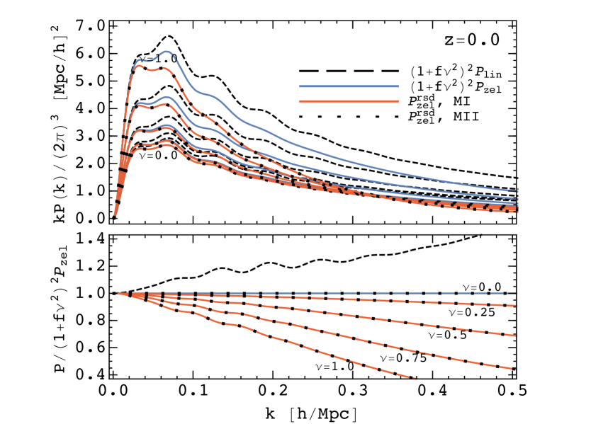
Figure 1: The redshift-space, Zeldovich power spectrum as a function of $k$ for select values of $\nu$ for $\Lambda$CDM at $z=0$. We highlight the agreement between the two series expansions MI (Eq. (4.9); red solid lines) and MII (Eq. (4.21); black dotted lines) described in the text. For comparison we show the linear theory results, $(1+f\nu^{2})^{2}P_{L}$, as the black dashed line and the real-space, Zel’dovich power spectrum multiplied by the linear RSD term $(1+f\nu^{2})^{2}$ as the blue lines. The upper panel shows the power spectrum, times $k$ to reduce the dynamic range, while the lower panel shows the ratio to $(1+f\nu^{2})P_{\rm Zel}$ which highlights the change in the damping as a function of $\nu$.

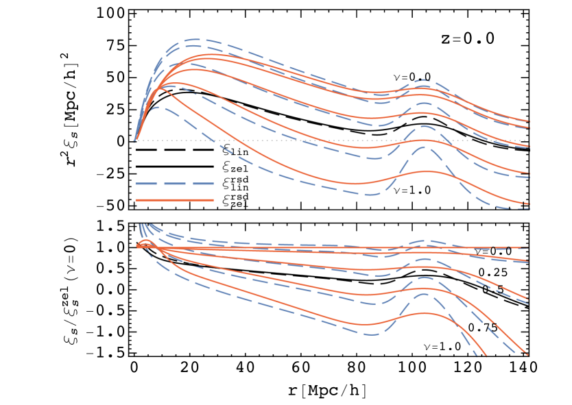
Figure 2: The redshift-space, Zeldovich correlation function as a function of $s$ for select values of $\nu$ for $\Lambda$CDM at $z=0$.

We evaluate the Zeldovich power spectrum and correlation function for the $\Lambda$cdm cosmology using the parameters $\Omega_{m}=0.295$, $\Omega_{b}=0.047$, $n_{s}=0.968$, $\sigma_{8}=0.835$ and $h=0.688$. Fig. 1 shows the power spectrum results, and the good agreement between MI and MII. At high $k$ we see the familiar damping of power from the Zeldovich dynamics, with the damping being larger along the line of sight than transverse to it. This damping corresponds to the fact that small scale structure does not form properly in the Zeldovich approximation. This is not of concern to us, since we are using the Zeldovich approximation for illustration. We are more interested in checking the self-consistency of the different approaches and the consistency of methods MI and MII. The two methods give excellent agreement on the scales of interest ($k<1\,h\,{\rm Mpc}^{-1}$), though on smaller scales differences begin to creep in that are due to our truncations in the sums in Eqs. (4.9) and (4.21). These differences could be reduced further by including more terms. For comparison we also show the deviations from linear theory, $(1+f\nu^{2})^{2}P_{L}$, as well as a phenomenological ‘Kaiser-Zeldovich’ approximation: $(1+f\nu^{2})^{2}P_{\rm Zel}$. The latter highlights how the damping in the Zeldovich approximation depends upon angle to the line of sight.

Since it will be useful later, we also reproduce the configuration-space 2-point function, $\xi(s,\nu)$, within the Zeldovich approximation. Fig. 2 shows $s^{2}\,\xi(s,\nu)$ for several values of $\nu$ with the characteristic BAO peak clearly visible at $s\simeq 100\,h^{-1}$Mpc. The BAO peak is broadened from its linear theory value by non-linear structure formation and that broadening is anisotropic. The angle-dependence of the Zeldovich correlation function is different from that of linear theory even at relatively large scales, showing that the Kaiser limit is approached very slowly in configuration space. We shall return to $\xi(s,\nu)$ in §5.

4.2 Moment expansion approach

In order to explore the moment expansion approach we return to the generating function. We are interested in ascertaining how well the moment expansion approach works compared to the exact result of the previous section. In other words, how many terms do we need to keep in the moment expansion in order to achieve good accuracy at the scales of interest? Since we are using leading order Lagrangian dynamics (the Zeldovich approximation) we can answer this question robustly as we can derive closed-form expressions for arbitrary velocity moments. Even though the full dynamics is not properly captured, we believe the answers will be relevant to the more general case as well.

We start from the expressions in Sec. 3.1 (setting $\delta_{a}(\mathbf{q})=\delta_{b}(\mathbf{q})=0$ since we are not interested in the biased tracers at this point), and use the cumulant expansion theorem (for Gaussian fields) to obtain

$$\widetilde{\mathcal{M}}(\mathbf{J},\mathbf{k}) =\frac{k^{3}}{2\pi^{2}}\int d^{3}q\ e^{i\mathbf{k}\cdot\mathbf{q}}\ e^{-\frac{1}{2}\left(k_{i}k_{j}+f(\mathbf{J}\cdot\hat{n})k_{\{i}\hat{n}_{j\}}+f^{2}(\mathbf{J}\cdot\hat{n})^{2}\hat{n}_{i}\hat{n}_{j}\right)A_{ij}}$$

$$=\frac{k^{3}}{2\pi^{2}}\int d^{3}q\ e^{i\mathbf{k}\cdot\mathbf{q}}\ e^{-\frac{1}{2}k_{i}k_{j}A_{ij}}e^{-\frac{1}{2}\left(fJ_{\hat{n}}\mathcal{A}+f^{2}J_{\hat{n}}^{2}\mathcal{B}\right)},$$ (4.22)

where we introduced $J_{\hat{n}}=\mathbf{J}\cdot\hat{n}$, $\mathcal{A}=k_{\{i}\hat{n}_{j\}}A_{ij}$ and $\mathcal{B}=\hat{n}_{i}\hat{n}_{j}A_{ij}$. Velocity moments in terms of the derivatives in $J_{\hat{n}}$ can now be obtained from the Taylor expansion

$$\widetilde{\mathcal{M}}(\mathbf{J},\mathbf{k})=\sum_{\ell=0}^{\infty}\frac{i^{\ell}}{\ell!}\left(J_{\hat{n}}\right)^{\ell}\widehat{\Xi}^{(\ell)}_{\hat{n}}(\mathbf{k}),\quad{\rm i.e.}\quad\widehat{\Xi}^{(\ell)}_{\hat{n}}(\mathbf{k})=(-i)^{\ell}\frac{\partial^{\ell}}{\partial J_{\hat{n}}^{\ell}}\widetilde{\mathcal{M}}(\mathbf{J},\mathbf{k})\Big{|}_{\mathbf{J}=0}.$$ (4.23)

We note that equivalently one could take the derivative relative to the logarithmic growth rate $f$ given that it always appears as $fJ_{\hat{n}}$ in Eq. (4.22) above. This guarantees that the $n^{\rm th}$ velocity moment is proportional to $f^{n}$, so the moment expansion can alternatively be considered as a Taylor expansion of the full RSD spectrum in powers of $f$ [69].

To obtain an explicit form for the moments it is useful to split them into odd and even groups. We write

$$\widetilde{\Xi}^{(2\ell)}_{\hat{n}}(k,\nu) =f^{2\ell}\sum_{m=0}^{\ell}\widetilde{\Xi}^{(2\ell)}_{m}(k)\ \nu^{2m}$$

$$=f^{2\ell}\sum_{n=0}^{\ell}\frac{(-1)^{n}}{2^{\ell+n}}\frac{(2\ell)!}{(\ell-n)!(2n)!}\int d^{3}q\ e^{i\mathbf{k}\cdot\mathbf{q}}~{}\mathcal{A}^{2n}\mathcal{B}^{\ell-n}e^{-\frac{1}{2}k_{i}k_{j}A_{ij}},$$

$$\widetilde{\Xi}^{(2\ell+1)}_{\hat{n}}(k,\nu) =if^{2\ell+1}\sum_{m=0}^{\ell}\widetilde{\Xi}^{(2\ell+1)}_{m}(k)\ \nu^{2m+1}$$

$$=if^{2\ell+1}\sum_{n=0}^{\ell}\frac{(-1)^{n}}{2^{\ell+n+1}}\frac{(2\ell+1)!}{(\ell-n)!(2n+1)!}\int d^{3}q\ e^{i\mathbf{k}\cdot\mathbf{q}}~{}\mathcal{A}^{2n+1}\mathcal{B}^{\ell-n}e^{-\frac{1}{2}k_{i}k_{j}A_{ij}},$$ (4.24)

where in the first lines we have separated the scale and angle dependence, implicitly defining the reduced velocity moments $\widetilde{\Xi}^{(\ell)}_{m}(k)$ via the $m^{\rm th}$ derivative of the moments themselves: $(1/m!)(\partial_{\nu})^{m}\widetilde{\Xi}^{(2\ell)}_{\hat{n}}(\mathbf{k})\big{|}_{\nu=0}$. The reduced moments are thus a function only of the amplitude of the wave vector, $k$. It is convenient to perform this separation since each moment contains only a finite number of powers of $\nu$, which can be seen explicitly in Refs. [38, 41] or Appendix A.

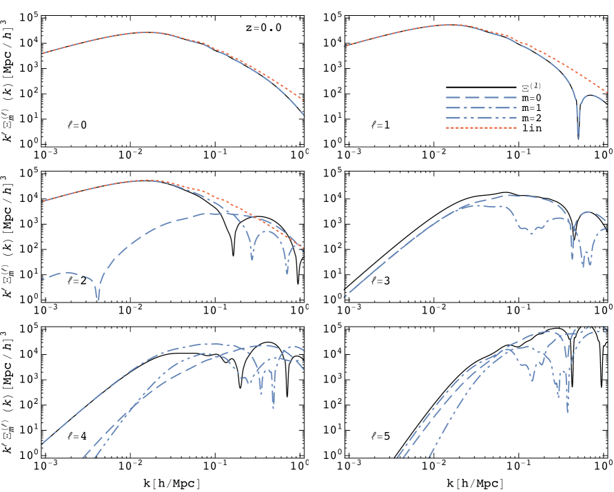
Figure 3: Velocity moments, $k^{\ell}\widetilde{\Xi}^{(\ell)}_{m}$, in Fourier space as a function of $k$, for $\Lambda$CDM at $z=0$. Moments are computed in Zeldovich approximation and separated according to the angular dependence (as in Eq. 4.25): $m=0$ (long dashed lines), $m=1$ (dash-dotted lines), $m=2$ (dash-dot-dotted lines). The black solid lines show the sum for $\nu=1$, i.e. each $m$-mode weighted maximally. The linear theory results are also shown for $\ell=0$, $1$ and $2$ (red dotted lines) and are each proportional to $P_{L}$.

We delegate the explicit derivation of the reduced velocity moments, $\widetilde{\Xi}^{(\ell)}_{m}(k)$, to Appendix B, where it is shown that

$$\widetilde{\Xi}^{(2\ell)}_{m}(k) =4\pi\sum_{s=0}^{\infty}\int q^{2}dq~{}e^{-\frac{1}{2}k^{2}(X+Y)}\xi^{(2\ell)}_{m,s}(k,X,Y)\left(\frac{kY}{q}\right)^{s}j_{s}(qk),$$

$$\widetilde{\Xi}^{(2\ell+1)}_{m}(k) =4\pi\sum_{s=0}^{\infty}\int q^{2}dq~{}e^{-\frac{1}{2}k^{2}(X+Y)}\xi^{(2\ell+1)}_{m,s}(k,X,Y)\left(\frac{kY}{q}\right)^{s}j_{s}(qk),$$ (4.25)

with the integrand functions given by

$$\xi^{(2\ell)}_{m,s}(X,Y) =\sum_{n=0}^{2\ell}\frac{F^{(2\ell)}_{m,n}(k,X,Y)}{(k^{2}Y/2)^{n}}U(-n,s-n+1,k^{2}Y/2),$$

$$\xi^{(2\ell+1)}_{m,s}(X,Y) =\sum_{n=0}^{2\ell+1}\frac{F^{(2\ell+1)}_{m,n}(k,X,Y)}{(k^{2}Y/2)^{n}}U(-n,s-n+1,k^{2}Y/2),$$ (4.26)

and the $F^{(\ell)}_{m,n}$ given explicitly by Eq. (B.8), with $U(a,b,z)$ is Tricomi’s confluent hypergeometric function as before.

Fig. 3 shows the first few velocity moments for $\Lambda$CDM at $z=0$. The red lines for $\ell=0$, 1 and 2 show the linear theory predictions which are all proportional to $P_{L}$ as plotted. We see that the Zeldovich solutions reduce to linear theory at low $k$ as expected (see below). Non-linear evolution changes the behavior at large $k$ and generates higher $\ell$ moments, which are highly suppressed at low $k$ in the way they are plotted here but become comparable to $\ell\leq 2$ for $k$ at or above the non-linear scale. By contrast the $\nu$ dependence is less straightforward. While $m\leq\ell$, the higher $m$ modes for a given $\ell$ are not suppressed at low $k$ in the way the higher $\ell$ modes are. For example for $\ell=2$ and $\ell=4$ (two lower left panels of Fig. 3) the $m=1$ mode dominates over $m=0$ and $m=2$ at low $k$. We shall compare this expansion to the others in §4.4.

In Eq. (4.24) we have expressed the velocity moments as an expansion in powers of $\nu$. It will be useful later to rearrange these expressions to give the multipole expansion of the moments. Using the relations

$$\nu^{2\ell}=\sum_{i=0}^{\ell}(-1)^{i}c^{{\rm e,}(\ell)}_{i}\mathcal{P}_{2i}(\nu),\qquad{\rm and}\qquad\nu^{2\ell+1}=\sum_{i=0}^{\ell}(-1)^{i}c^{{\rm o,}(\ell)}_{i}\mathcal{P}_{2i+1}(\nu),$$ (4.27)

where

$$c^{{\rm e,}(\ell)}_{n}=\frac{(-1)^{n}(4n+1)(2\ell)!}{2^{\ell-n}(\ell-n)!(2\ell+2n+1)!!},\qquad{\rm and}\qquad c^{{\rm o,}(\ell)}_{n}=\frac{(-1)^{n}(4n+3)(2\ell+1)!}{2^{\ell-n}(\ell-n)!(2\ell+2n+3)!!}.$$ (4.28)

we have straightforwardly the velocity moments in terms of Legendre polynomials

$$\widetilde{\Xi}^{(2\ell)}_{\hat{n}}(k,\nu) =f^{2\ell}\sum_{i=0}^{\ell}(-1)^{i}\left(\sum_{m=0}^{\ell}c^{{\rm e,}(m)}_{i}\widetilde{\Xi}^{(2\ell)}_{m}(k)\right)\mathcal{P}_{2i}(\nu),$$

$$\widetilde{\Xi}^{(2\ell+1)}_{\hat{n}}(k,\nu) =if^{2\ell+1}\sum_{i=0}^{\ell}(-1)^{i}\left(\sum_{m=0}^{\ell}c^{{\rm o,}(m)}_{i}\widetilde{\Xi}^{(2\ell+1)}_{m}(k)\right)\mathcal{P}_{2i+1}(\nu).$$ (4.29)

Finally we note that the moment expansion is particularly convenient for comparing to Eulerian methods. In particular it is easy to obtain the Kaiser result as indicated in Eq. (3.13), so let us derive the leading RSD contributions in this framework. We have

$$P_{s}(\mathbf{k}) =\widetilde{\Xi}^{(0)}_{\hat{n}}(\mathbf{k})+i\nu k\widetilde{\Xi}^{(1)}_{\hat{n}}(\mathbf{k})-\frac{1}{2}\nu^{2}k^{2}\widetilde{\Xi}^{(2)}_{\hat{n}}(\mathbf{k})+\ldots$$ (4.30)

$$=\int d^{3}r~{}e^{i\mathbf{k}\cdot\mathbf{r}}\left\langle\big{(}1+\delta(\mathbf{x})\big{)}\big{(}1+\delta(\mathbf{x}^{\prime})\big{)}\right\rangle+i\nu k\int d^{3}r~{}e^{i\mathbf{k}\cdot\mathbf{r}}\left\langle\big{(}1+\delta(\mathbf{x})\big{)}\big{(}1+\delta(\mathbf{x}^{\prime})\big{)}\Delta u_{\hat{n}}\right\rangle$$

$$\hskip 142.26378pt-\frac{1}{2}\nu^{2}k^{2}\int d^{3}r~{}e^{i\mathbf{k}\cdot\mathbf{r}}\left\langle\big{(}1+\delta(\mathbf{x})\big{)}\big{(}1+\delta(\mathbf{x}^{\prime})\big{)}\Delta u_{\hat{n}}^{2}\right\rangle+\ldots$$

$$=\int d^{3}r~{}e^{i\mathbf{k}\cdot\mathbf{r}}\left\langle\delta(\mathbf{x})\delta(\mathbf{x}^{\prime})\right\rangle+i\nu k\int d^{3}r~{}e^{i\mathbf{k}\cdot\mathbf{r}}\Big{(}\left\langle\delta(\mathbf{x}^{\prime})u_{\hat{n}}(\mathbf{x})\right\rangle-\left\langle\delta(\mathbf{x})u_{\hat{n}}(\mathbf{x}^{\prime})\right\rangle\Big{)}$$

$$\hskip 128.0374pt+\nu^{2}k^{2}\int d^{3}r~{}e^{i\mathbf{k}\cdot\mathbf{r}}\left\langle u_{\hat{n}}(\mathbf{x})u_{\hat{n}}(\mathbf{x}^{\prime})\right\rangle+\ldots,$$

where we have dropped terms proportional to Dirac $\delta$-functions. Assuming that the vector components of velocity can be neglected and only the scalar part contributes, i.e. we can write $\mathbf{v}(\mathbf{k})=(i\mathbf{k}/k^{2})\theta(\mathbf{k})$, and switching back to the peculiar velocity $\mathbf{v}=\mathcal{H}\mathbf{u}$ we get

$$P^{s}(\mathbf{k}) =P_{\delta\delta}(k)+i\nu k\mathcal{H}^{-1}\Big{(}P_{u_{\hat{n}}\delta}(\mathbf{k})-P_{\delta u_{\hat{n}}}(\mathbf{k})\Big{)}+\nu^{2}k^{2}\mathcal{H}^{-2}P_{u_{\hat{n}}u_{\hat{n}}}(\mathbf{k})$$

$$=P_{\delta\delta}(k)-2\nu^{2}\mathcal{H}^{-1}P_{\delta\theta}(k)+\nu^{4}\mathcal{H}^{-2}P_{\theta\theta}(k)\quad.$$ (4.31)

In linear theory $\theta=-f\mathcal{H}\delta$ so we have

$$P^{s}(\mathbf{k})=\big{(}1+f\nu^{2}\big{)}^{2}P_{L}(k),$$ (4.32)

i.e. the well known Kaiser formula [11]. The same limit can of course also be obtained via the direct Lagrangian approach, as argued in the earlier section, or from the streaming model by expanding the exponential and keeping only the leading, linear terms.

4.3 Streaming models

The streaming models arise from the cumulant expansion of $\mathcal{M}$ or $\widetilde{\mathcal{M}}$. In either space it is straightforward to show that $P_{s}(\mathbf{k})$ depends only upon even powers of $\nu=\hat{k}\cdot\hat{n}$, and that for any power of $\nu$ only a finite number of cumulants contribute. We shall be interested in how the expansion approaches the full Zeldovich result.

As mentioned above, there are two developments of the streaming model. One applies the cumulant theorem to the generating function in configuration space and the other to the generating function in Fourier space. Since the cumulants are constructed from the moments, and the moments are Fourier transform pairs, they in principle contain the same information if carried to infinite order. However, in practice, the non-local nature of the Fourier transform and the need to truncate the expansion at finite order makes their behavior very different, as we will show. First though we develop the streaming models more fully within the Zeldovich approximation.

4.3.1 Fourier space

The Gaussian streaming model in configuration space is well known (see earlier discussion and references) and will be developed in §4.3.2. The alternative formalism applies the cumulant expansion in Fourier space and is new to this paper. The extension of both the configuration-space and Fourier-space results beyond $2^{\rm nd}$ order is also new to this paper.

We can obtain cumulants from the $\widetilde{\Xi}^{(m)}_{\hat{n}}$ through Eq. (3.3.2). A general form of this transformation is given by

$$\widetilde{\mathcal{C}}^{(\ell)}_{\hat{n}}(k,\nu)=\sum_{i=1}^{\ell}\frac{(-1)^{i-1}(i-1)!}{\left[1+\Delta^{2}(k)\right]^{i}}B_{\ell,i}\left(\widehat{\Xi}^{(1)}_{\hat{n}}(k,\nu),\ldots,\widehat{\Xi}^{(\ell-i+1)}_{\hat{n}}(k,\nu)\right),$$ (4.33)

where $B_{\ell,i}\left(x_{1},\ldots,x_{\ell-i+1}\right)$ are partial Bell polynomials. The power spectrum is

$$\frac{k^{3}}{2\pi^{2}}P^{s}(k,\nu)=\left(1+\Delta^{2}\right)\exp\Bigg{[}i(\nu k)\widetilde{\mathcal{C}}^{(1)}_{\hat{n}}(k,\nu)-\frac{(\nu k)^{2}}{2}\widetilde{\mathcal{C}}^{(2)}_{\hat{n}}(k,\nu)+\ldots\Bigg{]}-1.$$ (4.34)

By analogy to the configuration space case, we can call the Gaussian streaming model (GSM) the truncation at the second cumulant $\widetilde{\mathcal{C}}^{(2)}_{\hat{n}}$ and dropping the higher ones. As noted previously, this form provides a huge simplifcation over the ‘usual’ streaming model result in that the connection between real and redshift space is algebraic. The structure of the redshift space terms is also particularly clear, and this form is reminiscent of the older ‘dispersion’ models which multiplied the linear theory result by a phenomenological damping [70, 71, 72, 73, 13, 74, 75, 36, 37]. We shall compare this expansion to the others in §4.4.

To bring out the correspondance with the dispersion models more clearly and to highlight the structure of the finger of god terms, let us consider $\mathcal{C}^{(2)}$ which derives from $\widetilde{\Xi}^{(2)}$. In PT $\widetilde{\Xi}^{(2)}$ contains a term going as $P_{L}\int P_{L}$, which is UV-sensitive. This gives a contribution to $\widetilde{\mathcal{C}}^{(2)}$ that looks like a constant. Thus a piece of $\mathcal{K}$ is $\exp[-k_{\parallel}^{2}\sigma^{2}]$ for some $\sigma^{2}$. On small scales $\Delta^{2}\gg 1$ and we have $P^{s}(k,\nu)\approx P(k)\exp[-k_{\parallel}^{2}\sigma^{2}]$, which is one of the common forms for the old dispersion models [70, 71]. It is interesting to note that the dispersion model approximation may explicitly break translational invariance (depending upon how $\sigma$ is computed) though this is preserved in the full cumulant form.

4.3.2 Configuration space

In order to obtain the streaming model in configuration space given in Sec. 3.3.1 we first need to obtain the configuration space ingredients, i.e. cumulants ${\mathcal{C}}^{(\ell)}_{\hat{n}}$ and moments $\Xi^{(\ell)}_{\hat{n}}$ in configuration space. We start by Fourier transforming the moments, using the angular dependence given in Eq. (4.24). We can write

$$\Xi^{(2\ell)}_{\hat{n}}\left(r,\hat{n}\cdot\hat{r}\right) =f^{2\ell}\sum_{m=0}^{\ell}\int\frac{d^{3}k}{(2\pi)^{3}}~{}\widetilde{\Xi}^{(2\ell)}_{m}(k)\left(\hat{k}\cdot\hat{n}\right)^{2m}e^{-i\mathbf{k}\cdot\mathbf{r}},$$

$$\Xi^{(2\ell+1)}_{\hat{n}}\left(r,\hat{n}\cdot\hat{r}\right) =if^{2\ell+1}\sum_{m=0}^{\ell}\int\frac{d^{3}k}{(2\pi)^{3}}~{}\widetilde{\Xi}^{(2\ell+1)}_{m}(k)\left(\hat{k}\cdot\hat{n}\right)^{2m+1}e^{-i\mathbf{k}\cdot\mathbf{r}}.$$ (4.35)

Using Legendre tensors defined by

$$\left\{\hat{r}_{i_{1}}\ldots\hat{r}_{i_{L}}\right\}^{L}_{\ell}=(2\ell+1)\int\frac{d\Omega_{k}}{4\pi}~{}\hat{k}_{i_{1}}\ldots\hat{k}_{i_{L}}\mathcal{P}_{\ell}\left(\hat{k}\cdot\hat{r}\right),$$ (4.36)

we have

$$\int\frac{d\Omega_{k}}{4\pi}~{}\hat{k}_{i_{1}}\ldots\hat{k}_{i_{L}}e^{-i\mathbf{k}\cdot\mathbf{r}}=\sum_{\ell=0}^{\infty}i^{\ell}j_{\ell}(kr)\left\{\hat{r}_{i_{1}}\ldots\hat{r}_{i_{L}}\right\}^{L}_{\ell}.$$ (4.37)

This leads to the useful angular integrals

$$\int\frac{d\Omega_{k}}{4\pi}~{}\left(\hat{k}\cdot\hat{n}\right)^{2L}e^{-i\mathbf{k}\cdot\mathbf{r}} =\sum_{\ell=0}^{L}c^{{\rm e,}(L)}_{\ell}\mathcal{P}_{2\ell}(\nu_{r})j_{2\ell}(kr),$$

$$\int\frac{d\Omega_{k}}{4\pi}~{}\left(\hat{k}\cdot\hat{n}\right)^{2L+1}e^{-i\mathbf{k}\cdot\mathbf{r}} =-i\sum_{\ell=0}^{L}c^{{\rm o,}(L)}_{\ell}\mathcal{P}_{2\ell+1}(\nu_{r})j_{2\ell+1}(kr),$$ (4.38)

where the coefficients $c^{{\rm e,}(L)}_{\ell}$ and $c^{{\rm o,}(L)}_{\ell}$ are given in Eq. (4.28). Finally we have for the configuration space velocity moments

$$\Xi^{(2\ell)}_{\hat{n}}\left(r,\nu_{r}\right) =f^{2\ell}\sum_{q=0}^{\ell}\mathcal{P}_{2q}(\nu_{r})\int\frac{k^{2}dk}{2\pi^{2}}~{}\left(\sum_{m=0}^{\ell}c^{{\rm e,}(m)}_{q}\widetilde{\Xi}^{(2\ell)}_{m}(k)\right)j_{2q}(kr),$$

$$\Xi^{(2\ell+1)}_{\hat{n}}\left(r,\nu_{r}\right) =f^{2\ell+1}\sum_{q=0}^{\ell}\mathcal{P}_{2q+1}(\nu_{r})\int\frac{k^{2}dk}{2\pi^{2}}~{}\left(\sum_{m=0}^{\ell}c^{{\rm o,}(m)}_{q}\widetilde{\Xi}^{(2\ell+1)}_{m}(k)\right)j_{2q+1}(kr).$$ (4.39)

In analogy to what we show in Fig. 3, angle multipoles of these velocity moments, $\Xi^{(\ell)}_{q}$, are shown in Fig. 4. Velocity moments, $\Xi^{(\ell)}_{\hat{n}}$, can of course be represented also in terms of power series in configuration space angles $\nu_{r}=\hat{n}\cdot\hat{r}$ by expanding the Legendre polynomials $\mathcal{P}_{\ell}$. The configuration space cumulants, ${\mathcal{C}}^{(\ell)}_{\hat{n}}$, are then given in terms of the moments, $\Xi^{(2\ell)}_{\hat{n}}$, by expressions analogous to Eq. (4.33).

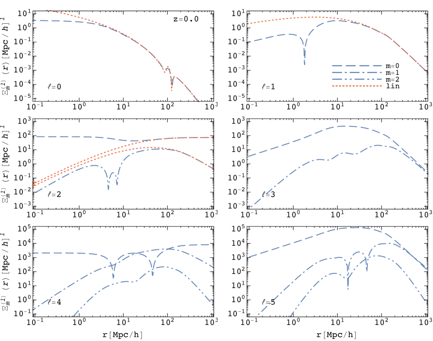
Figure 4: Velocity moments, $\Xi^{(\ell)}_{m}$ in configuration space as a function of $r$, for $\Lambda$CDM at $z=0$. Moments are computed in Zeldovich approximation and separated according to the angular dependence: $m=0$ (long dashed lines), $m=1$ (dash-dotted lines), $m=2$ (dash-dot-dotted lines). The linear theory results are also shown for $\ell=0$, $1$ and $2$ (red dotted lines) and are each proportional to $P_{L}$.

The redshift space power spectrum in terms of the configuration space streaming model is given by Eq. (3.17). The redshift space distortion effects are contained in the kernel $\mathcal{K}$, and given that $\xi(r)$ is isotropic the angular dependent kernel can be decomposed as

$$\ln\mathcal{K}(\mathbf{k},\mathbf{r})=\sum_{\ell=1}^{\infty}\frac{i^{\ell}}{\ell!}(k\nu)^{\ell}\mathcal{C}^{(\ell)}_{\hat{n}}(r,\mu)=\sum_{n=0}^{\infty}X_{n}\frac{\mu^{n}}{n!}=X_{0}+\ln\Bigg{[}\sum_{n=0}^{\infty}B_{n}\left(X_{1},\ldots,X_{n}\right)\frac{\mu^{n}}{n!}\Bigg{]}$$ (4.40)

where $B_{n}(X_{1},\ldots,X_{n})$ is the complete, exponential Bell polynomial and we have introduced angle series coefficients

$$X_{2m}(k,r,\nu) =(2m)!\sum_{\ell=1}^{\infty}\frac{(-1)^{\ell}}{(2\ell)!}(\nu fk)^{2\ell}\mathcal{C}^{(2\ell)}_{m}(r),$$

$$X_{2m+1}(k,r,\nu) =i(2m+1)!\sum_{\ell=0}^{\infty}\frac{(-1)^{\ell}}{(2\ell+1)!}(\nu fk)^{2\ell+1}\mathcal{C}^{(2\ell+1)}_{m}(r).$$ (4.41)

In analogy to the velocity moment decomposition in Eq. (4.24) we can decompose the cumulants as

$$\mathcal{C}^{(2\ell)}_{\hat{n}}(r,\mu) =f^{2\ell}\sum_{m=0}^{\ell}\mathcal{C}^{(2\ell)}_{m}(r)\mu^{2m},$$

$$\mathcal{C}^{(2\ell+1)}_{\hat{n}}(r,\mu) =f^{2\ell+1}\sum_{m=0}^{\ell}\mathcal{C}^{(2\ell+1)}_{m}(r)\mu^{2m+1}.$$

For the angular integration in the power spectrum expression, Eq. (3.17), we can now write

$$\int d\Omega_{r}\ e^{i\mathbf{k}\cdot\mathbf{r}}\mathcal{K}(\mathbf{k},\mathbf{r}) =e^{X_{0}}\sum_{L=0}^{\infty}\frac{1}{L!}B_{L}\left(X_{1},\ldots,X_{L}\right)\int d\Omega_{r}\ \mu^{L}e^{i\mathbf{k}\cdot\mathbf{r}}$$

$$=4\pi e^{X_{0}}\sum_{\ell=0}^{\infty}\mathcal{P}_{\ell}(\nu)\Bigg{[}\sum_{L=0}^{\infty}\frac{c^{(L)}_{\ell}}{L!}B_{L}\left(X_{1},\ldots,X_{L}\right)\Bigg{]}j_{\ell}(kr)$$ (4.42)

where the coefficient, $c^{(L)}_{\ell}$, is given by combining the odd and even coefficients given in Eq. (4.28). Explicitly we can write the values as

$$c^{(L)}_{\ell}=\frac{i^{\ell}(2\ell+1)L!}{2^{(L-\ell)/2}(\tfrac{1}{2}(L-\ell))!(L+\ell+1)!!}\begin{cases}1,~{}~{}{\rm if}~{}~{}L+\ell~{}~{}{\rm even}\\ 0,~{}~{}{\rm otherwise}\end{cases}.$$ (4.43)

Finally for the configuration space streaming model power spectrum we have

$$(2\pi)^{3}\delta^{K}(\mathbf{k})+P_{s}(\mathbf{k}) =\int d^{3}r\ e^{i\mathbf{k}\cdot\mathbf{r}}\big{[}1+\xi(r)\big{]}\mathcal{K}(\mathbf{k},\mathbf{r})$$ (4.44)

$$=4\pi\sum_{\ell=0}^{\infty}\mathcal{P}_{\ell}(\nu)\int r^{2}dr\ \big{[}1+\xi(r)\big{]}e^{X_{0}}\Bigg{[}\sum_{L=\ell}^{\infty}\frac{c^{(L)}_{\ell}}{L!}B_{L}\left(X_{1},\ldots,X_{L}\right)\Bigg{]}j_{\ell}(kr).$$

An alternative strategy for obtaining the power spectrum, taking into account just the Gaussian parts (i.e. truncation at the second cumulant), would be to directly transform the redshift space correlation function. This approach has been discussed in context of the linear theory results for density peaks in Ref. [76]. Extending this approach beyond the second cumulant depends on efficient evaluation of the streaming model correlation function, which we discuss in Sec. 5.4.

It is instructive to take the linear theory limit of the expression above. We start by writing the linear theory, configuration space velocity moments given in Eq. (4.39). Only first three velocity moments are non-vanishing. Moreover, given that $\widetilde{\Xi}^{(2)}_{0}$ has no contribution in linear theory and that $\Xi^{(0)}_{0}=P_{L}$, $\Xi^{(1)}_{0}=-2P_{L}/k$, $\Xi^{(2)}_{1}=-2P_{L}/k^{2}$, it follows

$$\Xi^{(0)}_{\hat{n}}\left(r,\nu\right) =\int\frac{k^{2}dk}{2\pi^{2}}~{}P_{L}(k)j_{0}(kr),$$ (4.45)

$$\Xi^{(1)}_{\hat{n}}\left(r,\nu\right) =-2f\nu\int\frac{kdk}{2\pi^{2}}~{}P_{L}(k)j_{1}(kr),$$

$$\Xi^{(2)}_{\hat{n}}\left(r,\nu\right) =-f^{2}\frac{2}{3}\int\frac{dk}{2\pi^{2}}~{}P_{L}(k)j_{0}(kr)-f^{2}\frac{2}{3}\left(1-3\nu^{2}\right)\int\frac{dk}{2\pi^{2}}~{}P_{L}(k)j_{2}(kr).$$

The configuration space velocity cumulants coincide with the moments in linear theory ($\mathcal{C}^{(0)}_{\hat{n}}=\Xi^{(0)}_{\hat{n}}$, $\mathcal{C}^{(1)}_{\hat{n}}\approx\Xi^{(1)}_{\hat{n}}$ and $\mathcal{C}^{(2)}_{\hat{n}}\approx\Xi^{(2)}_{\hat{n}}$) so using Eq. (4.41) we have

$$X_{0}=-\frac{1}{2}(\nu fk)^{2}\Xi^{(2)}_{0}(r)\quad,\quad X_{1}=i\nu fk\Xi^{(1)}_{0}(r)\quad{\rm and}\quad X_{2}=-(\nu fk)^{2}\Xi^{(2)}_{1}(r)\quad.$$ (4.46)

Collecting all this into Eq. (4.44) and using the explicit forms $B_{0}=1$, $B_{1}(X_{1})=X_{1}$ and $B_{2}(X_{1},X_{2})=X^{2}_{1}+X_{2}$, the linear theory power spectrum is given by

$$\frac{P_{s}(\mathbf{k})}{4\pi}=\int r^{2}dr\ \left[\xi(r)+X_{0}+\tfrac{1}{6}X_{2}\right]j_{0}(kr)+i\mathcal{P}_{1}(\nu)\int r^{2}dr\ X_{1}j_{1}(kr)-\frac{1}{3}\mathcal{P}_{2}(\nu)\int r^{2}dr\ X_{2}j_{2}(kr),$$

which upon using the integral representation of the Dirac delta function

$$\int r^{2}dr\ j_{n}(k^{\prime}r)j_{n}(kr)=\frac{\pi}{2k^{2}}\delta^{K}\left(k^{\prime}-k\right),$$ (4.47)

immediately gives the Kaiser result, $P_{s}(\mathbf{k})=\left(1+f\nu^{2}\right)^{2}P_{L}(k)$.

Finally, let us note that the computation procedure for the configuration space streaming model described in this section is not the only possibility. One alternative is to use methods already presented when computing the direct Lagrangian approach in Sec. 4.1. In particular the integrals given near Eq. (4.8) can be applied to solve the angular integral in Eq. (4.42). We have tried this and checked that the obtained results are consistent. We find that this leads to a somewhat more challenging numerical problem with slower convergence and thus we did not pursue this method further.

4.4 Comparison of different Fourier space methods

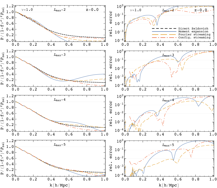
Figure 5: Comparison of different models in Fourier space, i.e. for the line-of-sight power spectrum. The left panels show the ratio of each model to the ‘Kaiser-Zeldovich’ model, to reduce the dynamic range for plotting purposes. The dashed black line indicates the full Zeldovich calculation, solid blue the moment expansion, dashed orange the Fourier-space streaming model and dot-dashed red the configuration-space streaming model. The right panels show the relative error, compared to the full Zeldovich calculation. The rows show how the convergence is improved by including more terms in the expansion, with the first row being the common ‘Gaussian’ approximation for the streaming models. See text for further discussion.

The line-of-sight power spectra for the different methods introduced in the previous sections are compared in Fig. 5. The left hand panels show the ratio of each expression to the ‘Kaiser-Zeldovich’ model, $P=(1+f\nu^{2})P_{\rm Zel}$, to reduce the dynamic range for plotting purposes. The right hand panels show the relative error in each expansion compared to the exact result (our direct Zeldovich expansion, shown as the dashed black line in the left panels). The different rows show how the convergence is improved by including more terms in the expansion with the first row being the common ‘Gaussian’ approximation for the streaming models. With our new formalism we are able to extend both the configuration-space and Fourier-space models beyond the $L_{\rm max}=2$/Gaussian approximation to assess the convergence of the cumulant expansion(s).

All models approach the correct answer, and linear theory, as $k\to 0$. On ‘linear scales’, $k<0.1\,h\,{\rm Mpc}^{-1}$, the models all perform at the percent level. However they deviate rapidly when moving to smaller scales. In general it appears the cumulant expansions out-perform the moment expansions at higher $k$, but the absolute performance of all of the models is relatively poor on these scales. All of the models show improvement when going beyond $L_{\rm max}=2$. While at low $k$ the moment expansion does as well as the cumulant expansion, the latter performs better at intermediate and high $k$ and converges slightly more quickly with increasing $L_{\rm max}$.

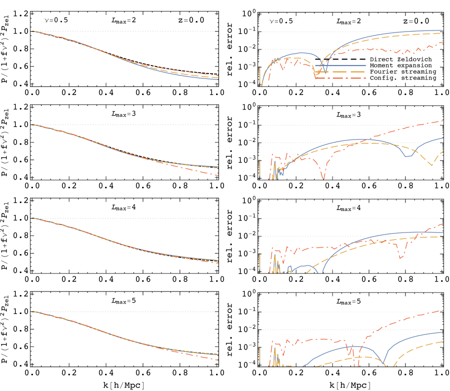
Figure 6: As for Fig. 5, but for $\nu=0.5$, i.e. a mode with $k_{z}=0.5\,k$. All of the models perform considerably better as $\nu$ is decreased, eventually approaching the exact result as $\nu\to 0$. See text for further discussion.

The line-of-sight power spectrum represents the worst-case scenario for the models, which all reproduce the transverse power spectrum exactly by construction. Fig. 6 is like Fig. 5, except for $\nu=0.5$. Note the relative error is much smaller in this case for all of the models. The moment expansion and the streaming models show sub-percent agreement with the full Zeldovich calculation well into the non-linear regime. The convergence of the expansions with increasing $L_{\rm max}$ is very rapid, with the streaming model showing fraction of a percent performance for all plotted scales by $L_{\rm max}=5$.

For all of the models we find that the errors are a strong function of $\nu$. Fig. 7 shows the same models as Figs. 5 and 6, but now at $k=0.1$ and $k=0.2\,h\,{\rm Mpc}^{-1}$ (both quasi-linear scales at $z=0$) as a function of $\nu$. The steep dependence of the error on $\nu$ is not too surprising, but could have consequences for comparison with observation. Observational probes which are restricted to high $\nu$, such as $21\,$cm interferometry in the presence of a foreground wedge [10], present a particular challenge for perturbation theory approaches. Similarly, methods for dealing with observational systematics which require modeling of high multipole moments (e.g. Ref. [77]) place stringent demands upon the theory. Conversely observational methods which downweight the line-of-sight modes (e.g. the $\hat{\xi}$ of Ref. [78]) could reduce the systematic error in comparison with theory while only modestly increasing the statistical error. An alternative, although similar, approach would be to include a ‘theoretical error’ [79] which is a steep function of $\nu$ when performing fits. We shall defer consideration of these approaches to future work.

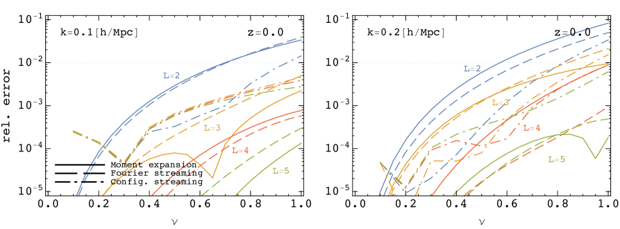
Figure 7: The error in the redshift-space power spectrum on quasi-linear scales (left: $k=0.1\,h\,{\rm Mpc}^{-1}$ and right: $k=0.2\,h\,{\rm Mpc}^{-1}$) as a function of $\nu=k_{z}/k$ for our different models (solid: moments, dashed: Fourier-space streaming and dot-dashed: configuration-space streaming). We see that the performance of all of the models is a strong function of $\nu$. All models have zero error as $\nu\to 0$ by construction, and every model performs significantly worse for $\nu\approx 1$ than for intermediate values of $\nu$. The configuration-space streaming model does well for small $L$, but the Fourier-space model improves most rapidly with increasing $L$. See text for further discussion and implications.

Finally, each of the models converges more quickly to the full result at high redshift than at low redshift. The relevant expansion parameter in this case is $fD$ rather than simply $D$ (the linear growth rate), and this actually peaks near $z\simeq 0.5$ for currently favored cosmological models. Figs. 8 and 9 show the relative error for each of our models at $\nu=1$ and $\nu=0.5$ for $z=1$ and $z=3$. Note by $z=3$ the best models are performing much better than a percent at $\nu=0.5$ over the entire range of scales shown, with the configuration-space streaming model achieving this even for $L_{\rm max}=2$. Even at $z=3$, however, the models have super-percent errors for $\nu=1$.

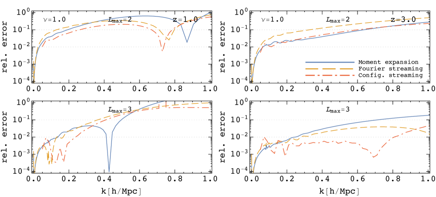
Figure 8: The error in our models at higher redshift. The lines are as in Fig. 5: solid blue for the moment expansion, dashed orange for the Fourier-space streaming model and dot-dashed red for the configuration-space streaming model. Plotted is the relative error at $\nu=1$ (i.e. the line of sight), compared to the full Zeldovich calculation, vs. $k$. The rows show $L_{\rm max}=2$ and $3$ to indicate how the convergence is improved by including more terms in the expansion (with the first row being the common ‘Gaussian’ approximation for the streaming models). The left panels show $z=1$ and the right panels $z=3$. See text for further discussion.

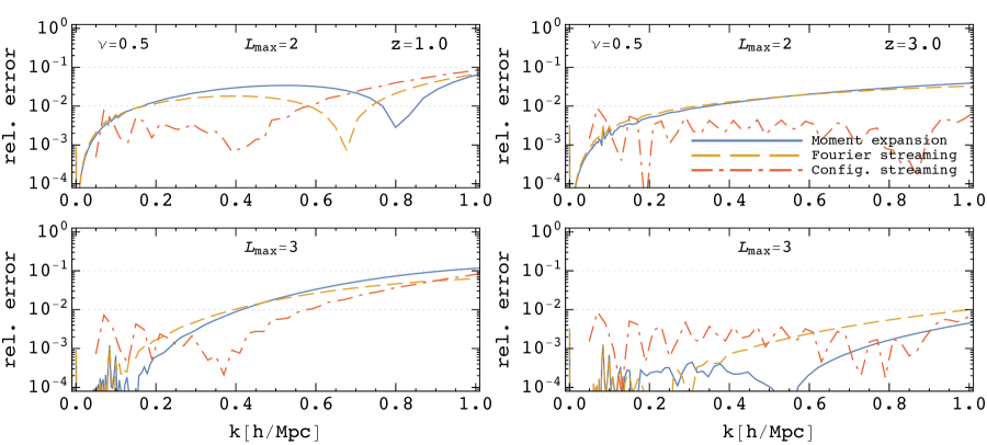
Figure 9: Same as figure 8 for $\nu=k_{z}/k=0.5$. All of the models perform better for lower $\nu$ at all redshifts. See text for further discussion.

5 Redshift-space distortions in configuration space

In this section we will consider the performance of each of our models in configuration space, i.e. for the redshift-space correlation function. We look at the convergence of the moment expansion approach as well as the two streaming models, compared to the full Zeldovich result. In particular we are able to go beyond leading terms in Fourier streaming model to look at the convergence of the cumulant expansion. In the case of the configuration space streaming model we shall stick to the Gaussian case, commenting later on what methods are required to efficiently move beyond this. As well as in the previous section, most of the tool developed to compute the cumulant and moment expansion are independent of the Zeldovich dynamics and are fully applicable in the full nonlinear case as well as in case of biased tracers (see §6).

5.1 Direct integration in configuration space

First we focus on obtaining directly the Zeldovich result for the RSD correlation function, given that it will serve as our benchmark result that we contrast to the other expansions. Obtaining the direct expression for Zeldovich RSD correlation function is relatively simple, since the two dimensional integration can be easily performed numerically. Given that the integral for $P(k)$ is Gaussian we have

$$\xi_{s}(\mathbf{r}) =\int\frac{d^{3}k}{(2\pi)^{3}}\ e^{-i\mathbf{k}\cdot\mathbf{r}}\int d^{3}q~{}e^{i\mathbf{k}\cdot\mathbf{q}}e^{-\frac{1}{2}k_{i}k_{j}A^{s}_{ij}}=\int\frac{d^{3}q}{(2\pi)^{3/2}\sqrt{{\rm det}A^{s}}}\ e^{\frac{1}{2}(\mathbf{q}-\mathbf{r})_{i}(\mathbf{q}-\mathbf{r})_{j}[A^{s}]^{-1}_{ij}},$$ (5.1)

where again $A^{s}_{ij}=R_{i\ell}R_{jm}A_{\ell m}$. The integrand in this case is not oscillatory and can be directly integrated in $\mathbf{q}$ variable, e.g. Ref. [25]. It is interesting to compare the structure of the integrand to its Fourier counterpart, $k_{i}k_{j}R_{i\ell}R_{jm}A_{\ell m}$, given in Eq. (4.5). First we note that if $\hat{k}\cdot\hat{n}\to 0$ one obtains the real space limit $k_{i}k_{j}R_{i\ell}R_{jm}A_{\ell m}=k^{2}\left(X+\mu^{2}Y\right)$, also if $f\to 0$. This does not happen in configuration space and we do not obtain the real space result for any value of $\hat{r}\cdot\hat{n}$. The limits $\hat{r}\cdot\hat{n}\to 0$ and $f\to 0$ are not the same. This is already clear from the form of the integral measure, $({\rm det}A^{s})=(1+f)^{2}X^{2}(X+Y)$, where no matter the value of $\hat{r}\cdot\hat{n}$, the $(1+f)^{2}$ factor is present. A similar thing happens for the term in exponent, $(\mathbf{q}-\mathbf{r})[A^{s}]^{-1}(\mathbf{q}-\mathbf{r})$. For this reason the error on the redshift-space correlation function does not have to go to zero as $\nu\to 0$.

Next we turn to looking at the performance of the three models; moment expansion, Fourier and configuration space streaming models in configuration space, and study the convergence focusing on Zeldovich dynamics as a guideline for more general cases.

5.2 Moment expansion in configuration space

In §4.2 we explored the moment expansion in Fourier space. To obtain results for the redshift-space correlation function corresponding to this expansion we can simply Fourier transform it. Given that the redshift-space correlation function is a Fourier transform of the redshift-space power spectrum, and the latter is given a sum of moments, the correlation function will also be given as a sum of Fourier transforms of the individual terms. Starting from Eq. (3.11) we have

$$\xi_{s}(\mathbf{r}) =\sum_{\ell=0}^{\infty}\frac{i^{\ell}}{\ell!}\int\frac{d^{3}k}{(2\pi)^{3}}\left(k\nu\right)^{\ell}\widetilde{\Xi}^{(\ell)}_{\hat{n}}(\mathbf{k})e^{-i\mathbf{k}.\mathbf{r}}\quad.$$ (5.2)

Using the expansion in the powers of $\nu$, given in Eq. (4.24), we have

$$\xi_{s}(\mathbf{r}) =\sum_{n=0}^{\infty}\mathcal{P}_{2n}(\nu_{r})\int\frac{k^{2}dk}{2\pi^{2}}\Bigg{[}\sum_{\ell=0}^{\infty}\frac{(-1)^{\ell}}{(2\ell)!}(fk)^{2\ell}\sum_{m=0}^{\ell}\bigg{(}c^{{\rm e,}(\ell+m)}_{n}\widetilde{\Xi}^{(2\ell)}_{m}(k)$$

$$\hskip 184.9429pt-\frac{fk}{2\ell+1}c^{{\rm e,}(\ell+m+1)}_{n}\widetilde{\Xi}^{(2\ell+1)}_{m}(k)\bigg{)}\Bigg{]}j_{2n}(kr).$$ (5.3)

We shall consider the convergence of this expression below. Before that we consider the linear (Kaiser) theory limit of this result. In linear theory only $\widetilde{\Xi}^{(0)}$, $\widetilde{\Xi}^{(1)}$ and $\widetilde{\Xi}^{(2)}$ contribute and we have

$$\xi_{s}(\mathbf{r}) =\sum_{n=0}^{\infty}\mathcal{P}_{2n}(\nu_{r})\Bigg{[}c^{{\rm e,}(0)}_{n}\int\frac{dk}{2\pi^{2}}k^{2}\widetilde{\Xi}^{(0)}_{0}(k)j_{2n}(kr)-f\int\frac{dk}{2\pi^{2}}k^{3}c^{{\rm e,}(1)}_{n}\widetilde{\Xi}^{(1)}_{0}(k)j_{2n}(kr)$$

$$\hskip 113.81102pt-\frac{1}{2}f^{2}\int\frac{dk}{2\pi^{2}}k^{4}\left(c^{{\rm e,}(1)}_{n}\widetilde{\Xi}^{(2)}_{0}(k)+c^{{\rm e,}(2)}_{n}\widetilde{\Xi}^{(2)}_{1}(k)\right)j_{2n}(kr)\Bigg{]}$$ (5.4)

Given the $c^{{\rm e,}\ell}_{n}$ coefficients in Eq. (4.28), and the fact that in linear theory $\Xi^{(2)}_{0}=0$, we have for the correlation function multipoles

$$\xi^{(2\ell)}_{s}(r) =\frac{4\ell+1}{2}\int_{-1}^{1}d\nu_{r}~{}\xi_{s}(\mathbf{r})\mathcal{P}_{2\ell}(\nu_{r})$$

$$=\int\frac{dk}{2\pi^{2}}k^{2}\left(c^{(0)}_{\ell}\widetilde{\Xi}^{(0)}_{0}(k)-fc^{(1)}_{\ell}k\widetilde{\Xi}^{(1)}_{0}(k)-\frac{1}{2}f^{2}c^{(2)}_{\ell}k^{2}\widetilde{\Xi}^{(2)}_{1}(k)\right)j_{2\ell}(kr).$$ (5.5)

Using again the linear theory expressions $\widetilde{\Xi}^{(0)}_{0}=P_{L}$, $\widetilde{\Xi}^{(1)}_{0}=-2P_{L}/k$ and $\widetilde{\Xi}^{(2)}_{1}=-2P_{L}/k^{2}$ it directly follows

$$\xi^{(0)}_{s}(r) =\left(1+\frac{2}{3}f+\frac{1}{5}f^{2}\right)\int\frac{k^{2}dk}{2\pi^{2}}~{}P_{L}(k)j_{0}(kr),$$

$$\xi^{(2)}_{s}(r) =-\left(\frac{4}{3}f+\frac{4}{7}f^{2}\right)\int\frac{k^{2}dk}{2\pi^{2}}~{}P_{L}(k)j_{2}(kr),$$

$$\xi^{(4)}_{s}(r) =\frac{8}{35}f^{2}\int\frac{k^{2}dk}{2\pi^{2}}~{}P_{L}(k)j_{4}(kr).$$ (5.6)

These results are, of course, in agreement with the well-known result that the Fourier and configuration space multipoles are simply linked by spherical Bessel transforms [12]

$$\xi^{(\ell)}_{s}(r)=i^{\ell}\int\frac{k^{2}dk}{2\pi^{2}}~{}P^{(\ell)}_{s}(k)j_{\ell}(kr)\quad,\quad P^{(\ell)}_{s}(k)=\frac{2\ell+1}{2}\int_{-1}^{1}d\nu~{}P_{s}(\mathbf{k})\mathcal{P}_{\ell}(\nu).$$ (5.7)

5.3 Fourier streaming models in configuration space

Next we move to the new Fourier version of the streaming model (§3.3.2). One of the simplifying features of this representation is that it can be transformed directly into configuration space (in contrast to the configuration-space streaming model where the translations are more complex). We present these results in this subsection. By Fourier transforming Eq. (4.34) we have

$$\xi_{s}(\mathbf{r}) =\int\frac{d^{3}k}{(2\pi)^{3}}P^{s}(k,\nu)e^{-i\mathbf{k}.\mathbf{r}}$$

$$=\int\frac{d^{3}k}{(2\pi)^{3}}~{}e^{-i\mathbf{k}.\mathbf{r}}\frac{2\pi^{2}}{k^{3}}\left(\left[1+\Delta^{2}(k)\right]\exp\left\{\sum_{\ell=1}^{\infty}\frac{i^{\ell}}{\ell!}(\nu k)^{\ell}\widetilde{\mathcal{C}}^{(\ell)}_{\hat{n}}(k,\nu)\right\}-1\right).$$ (5.8)

In order to proceed we need to compute the angular integral and thus we first collect the $\nu$ dependence in the exponent

$$\sum_{\ell=1}^{\infty}\frac{i^{\ell}}{\ell!}(k\nu)^{\ell}\mathcal{C}^{(\ell)}_{\hat{n}}(k,\nu) =\sum_{n=1}^{\infty}\nu^{2n}\sum_{\ell=1}^{\infty}\frac{(-1)^{\ell}}{(2\ell)!}(fk)^{2\ell}\left(\widetilde{\mathcal{C}}^{(2\ell)}_{n-\ell}(k)+\frac{2\ell}{fk}\widetilde{\mathcal{C}}^{(2\ell-1)}_{n-\ell}(k)\right)$$

$$=\sum_{m=1}^{\infty}Y_{m}(k)\frac{\nu^{m}}{m!},$$ (5.9)

where we have defined angle power coefficients, $Y_{m}$, in analogy to Eq. (4.41):

$$Y_{m}(k)=\left(1+(-1)^{m}\right)\frac{m!}{2}\sum_{\ell=1}^{\infty}\frac{(-1)^{\ell}}{(2\ell)!}(fk)^{2\ell}\left(\widetilde{\mathcal{C}}^{(2\ell)}_{m/2-\ell}(k)+\frac{2\ell}{fk}\widetilde{\mathcal{C}}^{(2\ell-1)}_{m/2-\ell}(k)\right).$$ (5.10)

This allows us to do the angular part of the $\mathbf{k}$ integral. Using Eq. (4.38)

$$\int\frac{d\Omega_{k}}{4\pi}\ e^{-i\mathbf{k}\cdot\mathbf{r}}\exp\Bigg{[}\sum_{\ell=1}^{\infty}\frac{i^{\ell}}{\ell!}(k\nu)^{\ell}\widetilde{\mathcal{C}}^{(\ell)}_{\hat{n}}(k,\nu)\Bigg{]} =\sum_{L=0}^{\infty}\frac{1}{L!}B_{L}\left(Y_{1},\ldots,Y_{L}\right)\sum_{\ell=0}^{\infty}(-1)^{\ell}c^{(L)}_{\ell}\mathcal{P}_{\ell}(\nu_{r})j_{\ell}(kr)$$

$$=\sum_{\ell=0}^{\infty}(-1)^{\ell}\mathcal{P}_{\ell}(\nu_{r})\Bigg{[}\sum_{L=0}^{\infty}\frac{c^{(L)}_{\ell}}{L!}B_{L}\left(Y_{1},\ldots,Y_{L}\right)\Bigg{]}j_{\ell}(kr),$$

where $B_{L}$ are again the Bell polynomials of order $L$. Note that the coefficients $c^{(L)}_{\ell}$ are identically zero if $\ell>L$, which limits the number of terms, i.e. the number of multipole moments, in the first sum above. This is of direct practical use since the truncation of the sum has to be enforced only in the $L$ variable. For the numerical implementations we consider below we find that truncation at $L\leq 10$ gives well converged results on scales above $\sim 1\,h^{-1}$Mpc.

The correlation function is thus given in terms of the Legendre polynomials that describe the angular dependence and scale dependent terms that are obtained as spherical Bessel transforms of the Fourier space quantities

$$\xi_{s}(\mathbf{r})=\int\frac{dk}{k}~{} \Delta^{2}(k)j_{0}(kr)$$ (5.11)

$$+\sum_{\ell=1}^{\infty}(-1)^{\ell}\mathcal{P}_{\ell}(\nu_{r})\int\frac{dk}{k}~{}\left(1+\Delta^{2}(k)\right)\Bigg{[}\sum_{L=1}^{\infty}\frac{c^{(L)}_{\ell}}{L!}B_{L}\left(Y_{1},\ldots,Y_{L}\right)\Bigg{]}j_{\ell}(kr).$$

Given the multipoles defined by Eq. (5.4), and that only even $\ell$ survive, we finally have

$$\xi^{(2\ell)}_{s}(r)=\int\frac{dk}{k}~{}\Bigg{(}\delta^{K}_{\ell,0} \Delta^{2}(k)+\left(1+\Delta^{2}(k)\right)\sum_{L=1}^{\infty}\frac{c^{{\rm e,}(L)}_{\ell}}{(2L)!}B_{2L}\left(0,Y_{2},0,\ldots,Y_{2L}\right)\Bigg{)}j_{2\ell}(kr),$$ (5.12)

where again the coefficients $c^{{\rm e,}(L)}_{\ell}$ are given by Eq. (4.28), $B_{L}$ are ordinary the Bell polynomials and the scale dependent functions, $Y_{2n}$, are given in Eq. (5.10) above.

As earlier it is instructive to see how the linear theory result emerges from the solution above. First we note that only two of the $Y_{2n}$ terms survive, explicitly $Y_{2}(k)=-2fk\widetilde{\mathcal{C}}^{(1)}_{0}(k)=4f\Delta_{L}^{2}(k)$ and $Y_{4}(k)=-12(fk)^{2}\widetilde{\mathcal{C}}^{(2)}_{1}(k)=24f^{2}\Delta_{L}^{2}(k)$. Keeping only the linearised contributions in the Bell polynomials we immediately regain the linear theory formula in the form

$$\xi^{(2\ell)}_{s}(r) =\left(\delta^{K}_{\ell,0}+2fc^{{\rm e,}(1)}_{\ell}+f^{2}c^{{\rm e,}(2)}_{\ell}\right)\int\frac{dk}{k}~{}\Delta_{L}^{2}j_{2\ell}(kr).$$ (5.13)

Using the values for the $c^{{\rm e,}(L)}_{\ell}$ coefficients, we promptly recover the linear configuration space multipoles given in Eq. (5.6).

5.4 Streaming models in configuration space

As a last expansion of the RSD contributions in configuration space we consider the configuration space streaming model introduced in §3.3.1. This method is the most challenging to evaluate beyond the second cumulant (Gaussian case), given that the methods needed differ from ones we have been developing so far. Brute force expansion in beyond Gaussian terms is of course possible but is labor intensive and does not guarantee fast convergence. An alternative is to use the Edgeworth expansion (proposed in e.g. Ref. [59] and studied in Ref. [80]) but we do not pursue this direction further here.

Fourier transforming the result from Eq. (3.17) we obtain

$$1+\xi_{s}(\mathbf{r})=\int d^{3}r^{\prime}\ \big{[}1+\xi(r^{\prime})\big{]}\int\frac{d^{3}k}{(2\pi)^{3}}e^{-i\mathbf{k}.\left(\mathbf{r}-\mathbf{r}^{\prime}\right)}\mathcal{K}(\mathbf{k},\mathbf{r}^{\prime}),$$ (5.14)

where the configuration streaming kernel is given by Eq. (3.16). Using the notation $\hat{n}\cdot\mathbf{k}=k_{\parallel}$ and $\hat{n}\cdot\mathbf{r}=r_{\parallel}$ and noting that the kernel, $\mathcal{K}$, depends only on $k_{\parallel}$ we can perform the integration in $\mathbf{k}_{\perp}=\mathbf{k}-k_{\parallel}\hat{n}$ to get

$$\int\frac{d^{3}k}{(2\pi)^{3}}e^{-i\mathbf{k}.\Delta\mathbf{r}}\mathcal{K}(\mathbf{k},\mathbf{r}-\Delta\mathbf{r})=\delta^{D}\left(\Delta\mathbf{r}_{\perp}\right)\int\frac{dk_{\parallel}}{2\pi}e^{-ik_{\parallel}\Delta r_{\parallel}}\mathcal{K}(k_{\parallel},\mathbf{r}-\Delta r_{\parallel}\hat{n}),$$ (5.15)

where the argument of the Dirac delta function is the perpendicular component $\mathbf{r}_{\perp}=\mathbf{r}-r_{\parallel}\hat{n}$. The full correlation function can thus be written as

$$1+\xi_{s}(\mathbf{r})=\int d\Delta r_{\parallel}\ \big{[}1+\xi\left(|\mathbf{r}-\Delta r_{\parallel}\hat{n}|\right)\big{]}\int\frac{dk_{\parallel}}{2\pi}e^{-ik_{\parallel}\Delta r_{\parallel}}\mathcal{K}(k_{\parallel},\mathbf{r}-\Delta r_{\parallel}\hat{n}),$$ (5.16)

where we can use $|\mathbf{r}^{\prime}|=|\mathbf{r}-\Delta r_{\parallel}\hat{n}|=\sqrt{r^{2}+\Delta r_{\parallel}^{2}-2r_{\parallel}\Delta r_{\parallel}}$ and $\hat{n}\cdot\mathbf{r}^{\prime}=\hat{n}\cdot(\mathbf{r}-\Delta r_{\parallel}\hat{n})=r_{\parallel}-\Delta r_{\parallel}=r\nu_{r}-\Delta r_{\parallel}$. Finally, the explicit result is given as

$$1+\xi_{s}(r,\nu_{r}) =\int\frac{dx\,dy}{2\pi}e^{-ixy}\ \Big{[}1+\xi\left(\sqrt{r^{2}+x^{2}-2\nu_{r}rx}\right)\Big{]}$$ (5.17)

$$\hskip 56.9055pt\times\exp\Bigg{[}\sum_{\ell=1}^{\infty}\frac{i^{\ell}}{\ell!}y^{\ell}\mathcal{C}^{(\ell)}_{\hat{n}}\left(\sqrt{r^{2}+x^{2}-2\nu_{r}rx},r\nu_{r}-x\right)\Bigg{]}.$$

Unfortunately, due to the oscillatory nature of the integrand this expression is not particularly useful in this form. We will not explore the general result further here, but will focus on the simpler case when cumulant expansion is truncated at second cumulant. In the case of $\ell\leq 2$ the integration in $y$ can be performed analytically giving

$$\int\frac{dy}{2\pi}e^{-iy\left(x-\mathcal{C}^{(1)}_{\hat{n}}\right)-\frac{1}{2}y^{2}\mathcal{C}^{(2)}_{\hat{n}}}=\frac{1}{\sqrt{2\pi\mathcal{C}^{(2)}_{\hat{n}}}}\exp\left\{-\left(x-\mathcal{C}^{(1)}_{\hat{n}}\right)^{2}/\left(2\mathcal{C}^{(2)}_{\hat{n}}\right)\right\},$$ (5.18)

and thus the correlation function is given by the standard result

$$1+\xi_{s}(r,\nu_{r})=\int_{-\infty}^{\infty}dx\ \frac{\Big{[}1+\xi\left(x,r,\nu_{r}\right)\Big{]}}{\sqrt{2\pi\mathcal{C}^{(2)}_{\hat{n}}\left(x,r,\nu_{r}\right)}}\exp\left\{-\frac{\left[x-\mathcal{C}^{(1)}_{\hat{n}}\left(x,r,\nu_{r}\right)\right]^{2}}{2\mathcal{C}^{(2)}_{\hat{n}}\left(x,r,\nu_{r}\right)}\right\}.$$ (5.19)

Given that we have derived the linear theory results in all the earlier cases it is natural to comment how the same result follows here. To this end it is not very convenient to use Eq. (5.19) directly, but instead we start from Eq. (5.14) and expand the exponential containing the cumulants. Linearising the cumulants (as done in the prior subsection for the Fourier streaming results) we get

$$1+\xi_{s}(\mathbf{r}) =\int\frac{d^{3}k}{(2\pi)^{3}}e^{-i\mathbf{k}.\mathbf{r}}\int d^{3}r^{\prime}\ e^{i\mathbf{k}\cdot\mathbf{r}^{\prime}}\big{[}1+\xi(r^{\prime})\big{]}\left(1+ik_{\parallel}\mathcal{C}^{(1)}_{\hat{n}}(\mathbf{r}^{\prime})-\frac{1}{2}k_{\parallel}^{2}\mathcal{C}^{(2)}_{\hat{n}}(\mathbf{r}^{\prime})\right)$$

$$=\int\frac{d^{3}k}{(2\pi)^{3}}e^{-i\mathbf{k}.\mathbf{r}}\left(1+\widetilde{\Xi}^{(0)}_{\hat{n}}(\mathbf{k})+ik_{\parallel}\widetilde{\Xi}^{(1)}_{\hat{n}}(\mathbf{k})-\frac{1}{2}k_{\parallel}^{2}\widetilde{\Xi}^{(2)}_{\hat{n}}(\mathbf{k})\right).$$ (5.20)

This is the familiar, linearized, moment expansion result. By using the multipoles we obtain the result in Eq. (5.5).

5.5 Comparison of models in configuration space

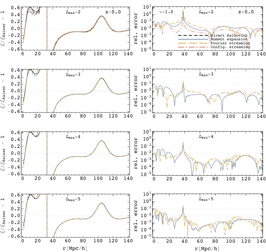
Figure 10: Comparison of the different models in configuration space, i.e. for the line-of-sight correlation function. This is the configuration-space analog of Fig. 5. As in that figure, the left panels show the ratio of each model to the ‘Kaiser-Zeldovich’ model (minus 1), to reduce the dynamic range for plotting purposes. The dashed black line indicates the full Zeldovich calculation, solid blue the moment expansion, dashed orange the Fourier-space streaming model and dot-dashed red the configuration-space streaming model. The right panels show the relative error, compared to the full Zeldovich calculation. The rows show how the convergence is improved by including more terms in the expansion, with the first row being the common ‘Gaussian’ approximation for the streaming models. Note that we have gone beyond the Gaussian streaming model in both Fourier and configuration space except for the configuration-space streaming model. See text for further discussion.

Finally we compare the different expansions, above, to the full Zeldovich calculation. Fig. 10 compares the different models to the full Zeldovich calculation for the line-of-sight correlation function, $\xi_{s}(r,\nu=1)$. In Fig. 11 and 12 equivalent plots are shown for the case $\xi_{s}(r,\nu=0.5)$ and $\xi_{s}(r,\nu=0.0)$ respectively. The figures show the absolute and relative convergence of the three approaches discussed in the earlier sections to the directly computed Zeldovich correlation function.

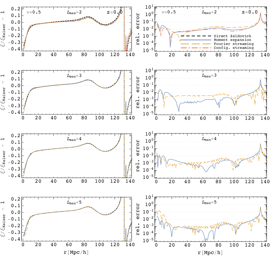
Figure 11: The same as Fig. 10 but for $\nu=0.5$.

As we found for the Fourier-space statistics, the models perform less well as $\nu\to 1$, with the error growing as a steep function of $\nu$. Unlike in the Fourier-space case we no longer expect zero error as $\nu\to 0$. Mirroring the discussion in §4.4 this could have implications for the way in which models are compared to data or the kinds of applications for which perturbative models are appropriate, but the details will differ from the Fourier-space case.

As mentioned earlier for the configuration space streaming model we performed only the $L=2$ Gaussian case calculation, and we find that already at $L_{\rm max}=2$ it performs at the level of $\sim 1\%$ precision on scales larger than $20\,h^{-1}$Mpc, outperforming both the moment expansion and the Fourier cumulant models (for $L_{\rm max}=2$) for all angles. The moment expansion performs very well, reaching subpercent accuracy for scales larger than $20\,h^{-1}$Mpc for $L_{\rm max}\leq 3$, and reaching sub-permille accuracy for $L_{\rm max}=5$. On these scales we see that Fourier streaming model is performing as well as the moment expansion for all angles and $L_{\rm max}$ values. The slight benefit of the Fourier streaming model can be noticed on scales smaller than $20\,h^{-1}$Mpc, where for $L_{\rm max}\geq 3$ it typically provides slightly better performance, i.e. faster convergence to the full result.

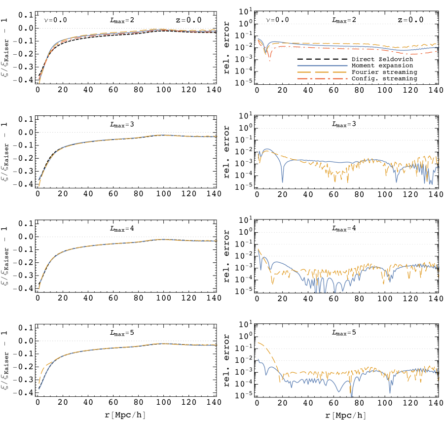
Figure 12: The same as Fig. 10 but for $\nu=0.0$.

6 Including bias expansion and non-linear dynamics

So far we have studied the effects of redshift-space mapping and explored the convergence properties of three different approaches within the Zeldovich approximation. As has been stressed before, our expansion and the mapping of cumulants and moments to the redshift-space power spectra and correlation functions are valid also in the fully nonlinear and biased case. In this section we provide the description for the first three moments in the Lagrangian Effective Field Theory (LEFT) context, taking into account biasing and nonlinear effects up to 1-loop. We study the density two point function, pairwise velocity and velocity dispersion. These quantities have been also studied in detail in the same framework in Ref. [16],and we repeat some of the derivations provided there but also provide the complete expression in Fourier space (Ref. [16] focused primarily on configuration space). The results presented here can be readily used with the expansion presented in the earlier sections, either in the Fourier or configuration space versions.

Since the Fourier space streaming model takes as ingredients velocity cumulants, it is useful to note that contributions up to the second cumulant (velocity dispersion) are the only non-vanishing contributions at one-loop PT. This also implies that working at the same PT order, all contributions to higher velocity moments come from disconnected graphs obtainable from these cumulants. This is, of course, related to the order counting in our PT prescription. Alternatively, one could organise the PT using as the leading order results from Sec. 4.1. There we show that linear displacements contribute to all of the velocity cumulants. Nonetheless, we will not pursue this line of investigation here and will leave it for future work.

We start the discussion by quickly reviewing the bias expansion, but for more detailed discussion we refer readers to Refs. [81, 82, 83, 84, 85]. Postulating that the number of biased objects is preserved by nonlinear evolution we have a continuity equation

$$(1+\delta_{a}(\mathbf{x},\tau))d^{3}x=(1+\delta_{a}(\mathbf{q},\tau_{\rm in}))d^{3}q,$$ (6.1)

Let us consider the biasing map $\delta_{a}(\mathbf{q},\tau_{\rm in})$, which we assume is a continuous and smooth function that can be expanded in powers of a characteristic (inverse distance) scale. In our case the scale will be the Lagrangian radius of the biased object (e.g. a protohalo) with associated wavenumber $k_{L}$. If we choose the initial time $\tau_{\rm in}$ early enough, all the dark matter fields in the problem can be considered as linear. An extensive list of bias parameters in Lagrangian space can be found in Ref. [85]. The first few terms are

$$\delta_{a}(\mathbf{q}) =b_{\delta}~{}:\delta_{L}:(\mathbf{q})$$

$$~{}+b_{\delta^{2}}:\delta^{2}_{L}:(\mathbf{q})+b_{s^{2}}:s_{L}^{2}:(\mathbf{q})$$

$$~{}+b_{\delta^{3}}:\delta^{3}_{L}:(\mathbf{q})+b_{\delta s^{2}}:\delta_{L}:(\mathbf{q}):s^{2}_{L}:(\mathbf{q})+b_{s^{3}}:s^{3}_{L}:(\mathbf{q})$$

$$~{}+b_{\partial^{2}\delta}\frac{\partial_{q}^{2}}{k_{L}^{2}}:\delta_{L}:(\mathbf{q})+{\rm``stochastic"}+\ldots$$ (6.2)

where $:O:$ represents the renormalised bias term (these will be defined explicitly further below), and $k_{L}$ is a characteristic physical scale related to Lagrangian halo radius. We have also defined the shear operator

$$\hat{s}_{ij}(\mathbf{q})=\frac{\partial_{i}\partial_{j}}{\partial^{2}}-\frac{1}{3}\delta^{K}_{ij},~{}~{}~{}{\rm and~{}the~{}corresponding~{}Fourier~{}operator~{}is}~{}~{}\hat{s}_{ij}(\mathbf{p})=\frac{p_{i}p_{j}}{p^{2}}-\frac{1}{3}\delta^{K}_{ij}.$$

Note that, by construction, independent third order bias terms like the $\psi$, vanish in the initial conditions if we restrict ourselves to linear initial dynamics. This means that terms of this form, in this bias picture where biasing is set in the initial conditions, arise in Eulerian space only due to nonlinear evolution, and thus should not be considered as free biasing coefficients (this is analogous to the so-called ‘co-evolution picture’). We use the notation

$$s_{L,ij}(\mathbf{q}) =\hat{s}_{ij}(\mathbf{q})\delta_{L}(\mathbf{q})=\left(\frac{\partial_{i}\partial_{j}}{\partial^{2}}-\frac{1}{3}\delta^{K}_{ij}\right)\delta_{L}(\mathbf{q})$$ (6.3)

and also define renormalised operators, where the trivial zero-lag parts are subtracted from the higher operators, so that:

$$:\delta_{L}: =\delta_{L},$$

$$:\delta_{L}^{2}: =\delta_{L}^{2}-\left\langle\delta_{L}^{2}\right\rangle=\delta_{L}^{2}-\sigma_{L}^{2},$$

$$:s_{L}^{2}: =s_{L}^{2}-\left\langle s_{L}^{2}\right\rangle=s_{L}^{2}-\tfrac{2}{3}\sigma_{L}^{2},$$

$$:\delta_{L}^{3}: =\delta_{L}^{3}-3\left\langle\delta_{L}^{2}\right\rangle\delta_{L}-\left\langle\delta_{L}^{3}\right\rangle=\delta_{L}^{3}-3\sigma_{L}^{2}\delta_{L},$$

$$:s_{L}^{3}: =s_{L}^{3}-\left\langle s_{L}^{3}\right\rangle=s_{L}^{3},$$ (6.4)

An alternative would be to use the biasing prescription given in e.g. Ref. [23] (see also Ref. [86] for recent discussion), where the biases are defined in full resummed form, rather then perturbatively. In terms of generating functions we can rewrite the given density field

$$\delta_{a}(\mathbf{q}) =\hat{\delta}_{a}(\lambda,\gamma,\eta)e^{i\lambda\delta_{L}(\mathbf{q})+i\gamma s^{2}_{L}(\mathbf{q})+i\eta s^{3}_{L}(\mathbf{q})}\Big{|}_{\lambda=\gamma=\eta=0},$$

where $\hat{\delta}_{a}(\lambda,\gamma,\eta)$ is the biasing operator acting on the bias generating function $\exp[i\lambda\delta_{L}+i\gamma s^{2}_{L}+i\eta s^{3}_{L}]$. Explicitly we can write

$$1+\hat{\delta}_{a}(\lambda,\gamma,\eta)=1 -i\left(b_{\delta}-3\sigma_{L}^{2}b_{\delta^{3}}\right)\partial_{\lambda}-b_{\delta^{2}}\left(\partial^{2}_{\lambda}+\sigma_{L}^{2}\right)+ib_{\delta^{3}}\partial^{3}_{\lambda}$$

$$-ib_{s^{2}}\partial_{\gamma}-b_{\delta s^{2}}\partial_{\lambda}\partial_{\gamma}-ib_{s^{3}}\partial_{\eta}$$

$$-ib_{\partial^{2}\delta}\frac{\partial_{q}^{2}}{k_{L}^{2}}\partial_{\lambda}+{\rm``stochastic"}+\ldots.$$ (6.5)

The generating function for any cross-moments of pairwise velocity for two generic biased tracers in terms of the displacement field then generalizes to

$$1+\mathcal{M}_{ab}\big{(}\mathbf{J},\mathbf{r}\big{)} =\int\frac{d^{3}k}{(2\pi)^{3}}d^{3}q~{}e^{-i\mathbf{k}\cdot(\mathbf{r}-\mathbf{q})}~{}\left\langle\big{[}1+\delta_{a}(\mathbf{q})\big{]}\big{[}1+\delta_{b}(\mathbf{q})\big{]}\exp\Big{[}i\mathbf{k}\cdot\Delta(\mathbf{q})+iJ^{j}\Delta^{\prime}_{j}(\mathbf{q})\Big{]}\right\rangle$$

$$=\big{[}1+\hat{\delta}_{a}(\lambda_{1},\gamma_{1},\eta_{1})\big{]}\big{[}1+\hat{\delta}_{b}(\lambda_{2},\gamma_{2},\eta_{2})\big{]}\int\frac{d^{3}k}{(2\pi)^{3}}d^{3}q~{}e^{-i\mathbf{k}\cdot(\mathbf{r}-\mathbf{q})}~{}\left\langle e^{iX}\right\rangle\bigg{|}_{\lambda=\gamma=\lambda=0},$$

where

$$X=\lambda_{1}\delta_{L}(\mathbf{q}_{1})+\lambda_{2}\delta_{L}(\mathbf{q}_{2}) +\gamma_{1}s_{L}^{2}(\mathbf{q}_{1})+\gamma_{2}s_{L}^{2}(\mathbf{q}_{2})$$

$$+\eta_{1}s_{L}^{3}(\mathbf{q}_{1})+\eta_{2}s_{L}^{3}(\mathbf{q}_{2})+\mathbf{k}\cdot\Delta(\mathbf{q})+J^{j}\Delta^{\prime}_{j}(\mathbf{q}).$$ (6.6)

This provides us with the means to compute the moments, and thus the cumulants, for biased tracers up to the terms we used in the bias expansion.

Let us focus for a moment on the stochastic term. In Lagrangian coordinates we are trying to describe the overdensity of discrete objects in terms of continuous dark matter fields. In order to be able to achieve that an auxilliary stochastic field, $\epsilon$, has to be added to the set of our bias operators. Intuitively, if we are describing very sparse objects this field has to play the role of noise. Thus we can write

$$\delta_{a}(\mathbf{q})=\bar{\delta}_{a}(\mathbf{q})+\epsilon_{a}(\mathbf{q}),$$ (6.7)

where $\bar{\delta}_{a}(\mathbf{q})$ is the average over the stochastic distribution, i.e. assuming we have a PDF, $p_{a}[\epsilon]$, associated with the random variable $\epsilon$ such that $\int[\mathcal{D}\epsilon]\epsilon p_{a}[\epsilon]=0$, we have

$$\bar{\delta}_{a}(\mathbf{q},\tau)=\int[\mathcal{D}\epsilon]\delta_{a}(\mathbf{q},\tau)p_{a}[\epsilon](\mathbf{q},\tau).$$ (6.8)

For $\bar{\delta}_{a}$ we can assume the usual bias expansion in terms of the operators in Eq. (6.4). For the field in the Eulerian coordinates we then have

$$(2\pi)^{3}\delta^{D}(\mathbf{k})+\delta_{a}(\mathbf{k}) =\int d^{3}q~{}e^{i\mathbf{k}\cdot\mathbf{q}}~{}\left[1+\delta_{a}(\mathbf{q})\right]e^{i\mathbf{k}\cdot\Psi(\mathbf{q})}$$ (6.9)

$$=\int d^{3}q~{}e^{i\mathbf{k}\cdot\mathbf{q}}~{}\left[1+\bar{\delta}_{a}(\mathbf{q})\right]e^{i\mathbf{k}\cdot\Psi(\mathbf{q})}+\int d^{3}q~{}e^{i\mathbf{k}\cdot\mathbf{q}}~{}\epsilon_{a}(\mathbf{q})e^{i\mathbf{k}\cdot\Psi(\mathbf{q})}.$$

Given that, by construction, the stochastic field does not correlate with the $\bar{\delta}_{a}$, this gives us the auto power spectrum

$$(2\pi)^{3}\delta^{D}(\mathbf{k})+P_{a}(k) =\int d^{3}q~{}e^{i\mathbf{k}\cdot\mathbf{q}}~{}\left\langle\left[1+\bar{\delta}_{a}(\mathbf{q}_{1})\right]\left[1+\bar{\delta}_{a}(\mathbf{q}_{2})\right]e^{i\mathbf{k}\cdot\Delta(\mathbf{q},\tau)}\right\rangle$$

$$\hskip 113.81102pt+\int d^{3}q~{}e^{i\mathbf{k}\cdot\mathbf{q}}~{}\left\langle\epsilon_{a}(\mathbf{q}_{1})\epsilon_{a}(\mathbf{q}_{2})e^{i\mathbf{k}\cdot\Delta(\mathbf{q},\tau)}\right\rangle$$ (6.10)

Focusing on the last term, and assuming also that $\Delta$ and $\epsilon_{a}$ are uncorrelated to be consistent with the definition of $\epsilon_{a}$, we can introduce $\left\langle\epsilon_{a}(\mathbf{q}_{1})\epsilon_{a}(\mathbf{q}_{2})\right\rangle^{\prime}=\xi_{\epsilon_{a}}(\mathbf{q})$. Assuming Poisson statistics for $\epsilon_{a}$ we have a constant Fourier space variance, i.e. $\xi_{\epsilon_{a}}(\mathbf{q})\sim\delta^{D}(\mathbf{q})$. Thus

$$\int d^{3}q~{}e^{i\mathbf{k}\cdot\mathbf{q}}~{}\xi_{\epsilon_{a}}(\mathbf{q},\tau)\left\langle e^{i\mathbf{k}\cdot\Delta(\mathbf{q},\tau)}\right\rangle\sim{\rm const}_{a}~{}\left\langle e^{i\mathbf{k}\cdot\Delta(\mathbf{q},\tau)}\right\rangle_{\mathbf{q}\to 0}\sim{\rm const}_{a}.$$ (6.11)

It is interesting to note that the constant term, under the assumptions above, is not sensitive to RSD and should have the same value for all angle bins (or equivalently, contribute only to $\ell=0$). The noise should depend only on the tracer type (thus the $a$ label on the constant). If we allow a correlation with the stochastic contributions to the dynamical fields, $\Delta$, it should be clear from above that we will get additional scale dependence and that will, of course, also affect redshift space. Moreover, similar analysis can be performed if we have scale-dependent stochasticity $\xi^{\prime}_{\epsilon_{a}}(\mathbf{q})\sim\partial^{2}/k_{\epsilon}^{2}\delta^{D}(\mathbf{q})$. From there we can also conclude that such terms, even though they carry new bias coefficients, should not be affected by the redshift space mapping (under the assumptions above). One caveat to this statement is the possibility of anisotropic selection effects (e.g. Ref. [87]), which would introduce additional line-of-sight-dependent bias operators and stochastic components (e.g. Ref. [53]). These terms arise from survey non-idealities rather than dynamical processes and their impact would need to be addressed on a case-by-case basis.

6.1 Two point function in real space

In this subsection we focuse on providing the theory for the two point halo correlation function and power spectrum in real space. Formally this is the zeroth moment of the real space generating function

$$\xi_{ab}=\Xi_{0}(\mathbf{r})=1+\mathcal{M}_{ab}\big{(}\mathbf{J}=0,\mathbf{r}\big{)}.$$ (6.12)

Using the Lagrangian framework we have set up and applying the cumulant expansion at 1-loop we see that we get contributions only from the first two cumulants

$$\log\left\langle e^{iX}\right\rangle=\sum_{n=2}^{\infty}\frac{i^{n}}{n!}\left\langle X^{n}\right\rangle_{c}=-\frac{1}{2}\left\langle X^{2}\right\rangle_{c}-\frac{i}{6}\left\langle X^{3}\right\rangle_{c}+\ldots.$$ (6.13)

Given that terms involving third order shear field $s_{L}^{3}$ do not contribute at 1-loop and we have

$$-\frac{1}{2}\left\langle X^{2}\right\rangle_{c}= -\frac{1}{2}k_{i}k_{j}A_{ij}-\lambda_{1}\lambda_{2}\xi_{L}-(\lambda_{1}+\lambda_{2})k_{i}U^{10}_{i}$$

$$-\gamma_{1}\gamma_{2}\zeta_{L}-(\gamma_{1}+\gamma_{2})k_{i}V^{10}_{i}-\frac{1}{2}(\lambda_{1}^{2}+\lambda_{2}^{2})\sigma_{\delta_{L}}^{2}$$

$$-\frac{i}{6}\left\langle X^{3}\right\rangle_{c}= -\frac{i}{6}k_{i}k_{j}k_{l}W_{ijk}-i\lambda_{1}\lambda_{2}k_{i}U^{11}_{i}-\frac{i}{2}(\lambda_{1}+\lambda_{2})k_{i}k_{j}A^{10}_{ij}-\frac{i}{2}\left(\lambda_{1}^{2}+\lambda_{2}^{2}\right)k_{i}U^{20}_{i}$$

$$-\frac{i}{2}(\gamma_{1}+\gamma_{2})k_{i}k_{j}A^{20}_{ij}-i(\gamma_{1}\lambda_{1}+\gamma_{2}\lambda_{2})k_{i}V^{11}_{i}-i(\gamma_{1}\lambda_{2}+\gamma_{2}\lambda_{1})k_{i}V^{12}_{i}$$

$$-i(\gamma_{1}\lambda_{1}\lambda_{2}+\gamma_{2}\lambda_{1}\lambda_{2})\chi^{11}-\frac{i}{2}(\gamma_{1}\lambda_{2}^{2}+\gamma_{2}\lambda_{1}^{2})\chi^{12}-\frac{i}{2}(\gamma_{1}\lambda_{1}^{2}+\gamma_{2}\lambda_{2}^{2})\sigma^{4}_{\delta_{L}^{2}s^{2}_{L}},$$ (6.14)

where we have introduced $\sigma^{4}_{\delta_{L}^{2}s^{2}_{L}}=\left\langle\delta_{L}^{2}s_{L}^{2}\right\rangle_{c}$, and we have [16]

$$A_{ij} =\left\langle\Delta_{i}\Delta_{j}\right\rangle_{c},~{}~{}\xi_{L}=\left\langle\delta_{L1}\delta_{L2}\right\rangle_{c},~{}~{}U^{10}_{i}=\left\langle\delta_{L}\Delta_{i}\right\rangle_{c},~{}~{}\zeta_{L}=\left\langle s^{2}_{L1}s^{2}_{L2}\right\rangle_{c},~{}~{}V^{10}_{i}=\left\langle s^{2}_{L}\Delta_{i}\right\rangle_{c},$$

$$W_{ijk} =\left\langle\Delta_{i}\Delta_{j}\Delta_{l}\right\rangle_{c},~{}~{}U^{11}_{i}=\left\langle\delta_{L1}\delta_{L2}\Delta_{i}\right\rangle_{c},~{}~{}A^{10}_{ij}=\left\langle\delta_{L}\Delta_{i}\Delta_{j}\right\rangle_{c},~{}~{}U^{20}_{i}=\left\langle\delta_{L}^{2}\Delta_{i}\right\rangle_{c},$$

$$\hskip 73.97733ptA^{20}_{ij}=\left\langle s^{2}_{L}\Delta_{i}\Delta_{j}\right\rangle_{c},~{}V^{11}_{i}=\left\langle s_{L1}^{2}\delta_{L1}\Delta_{i}\right\rangle_{c},~{}V^{12}_{i}=\left\langle s_{L1}^{2}\delta_{L2}\Delta_{i}\right\rangle_{c},$$

$$\hskip 73.97733pt\chi^{11}=\left\langle s_{L1}^{2}\delta_{L1}\delta_{L2}\right\rangle_{c},~{}\chi^{12}=\left\langle s_{L1}^{2}\delta_{L2}^{2}\right\rangle_{c}.$$ (6.15)

This produces a number of cross and auto correlators of the bias operators and displacement field. The purely displacement terms, $A_{ij}$ and $W_{ijk}$, are the same as in the unbiased case (i.e. the dark matter case) and we refer the reader to Ref. [30] for a detailed discussion of this case. Terms represented by $\xi_{L}$, $\zeta_{L}$ and $\chi^{12}$ ($\chi^{11}$ does not contribute) are pure bias correlation terms, and describe the proto-field of a biased tracer. The rest of the terms are correlations of bias terms and dynamical displacement terms.

Acting with the biasing operators on the cumulants and expanding all but linear displacements up to 1-loop order we have

$$\big{[}1 +\hat{\delta}_{a}(\lambda_{1},\gamma_{1},\eta_{1})\big{]}\big{[}1+\hat{\delta}_{b}(\lambda_{2},\gamma_{2},\eta_{2})\big{]}\left\langle e^{iX}\right\rangle=e^{-\frac{1}{2}k_{i}k_{j}A_{L,ij}}\Bigg{\{}1-\frac{1}{2}k_{i}k_{j}A^{\rm loop}_{ij}-\frac{i}{6}k_{i}k_{j}k_{l}W^{\rm loop}_{ijk}$$

$$~{}~{}~{}-b_{\delta,\{a,b\}}\Big{(}k_{i}k_{j}A^{10}_{ij}-2ik_{i}U^{10}_{i}\Big{)}+b_{\delta,a}b_{\delta,b}\Big{(}\xi_{L}+ik_{i}U^{11}_{i}-k_{i}k_{j}U^{10}_{i}U^{10}_{j}\Big{)}$$

$$~{}~{}~{}+b_{\delta^{2},\{a,b\}}\Big{(}ik_{i}U^{20}_{i}-k_{i}k_{j}U^{10}_{i}U^{10}_{j}\Big{)}+b_{\delta^{2},\{a}b_{\delta,b\}}\Big{(}2ik_{i}U^{10}_{i}\xi_{L}\Big{)}+b_{\delta^{2},a}b_{\delta^{2},b}\bigg{(}\frac{1}{2}\xi_{L}^{2}\bigg{)}$$

$$~{}~{}~{}-b_{s^{2},\{a,b\}}\Big{(}k_{i}k_{j}A^{20}_{ij}-2ik_{i}V^{10}_{i}\Big{)}+b_{\delta,\{a}b_{s^{2},b\}}\Big{(}2ik_{i}V^{12}_{i}\Big{)}+b_{s^{2},\{a}b_{\delta^{2},b\}}\chi^{12}+b_{s^{2},a}b_{s^{2},b}\zeta_{L}$$

$$~{}~{}~{}-\frac{1}{2}\alpha_{0}k^{2}+ib_{\partial^{2}\delta,\{a,b\}}\bigg{(}2k_{i}\frac{\partial^{2}}{k_{L}^{2}}U^{(1)}_{i}\bigg{)}+b_{\delta,\{a}b_{\partial^{2}\delta,b\}}\Big{(}2\frac{\partial^{2}}{k_{L}^{2}}\xi_{L}\Big{)}+\ldots\Bigg{\}}+{\rm``stochastic"},$$ (6.16)

where we introduced the notation $b_{\{a,b\}}=\frac{1}{2}(b_{a}+b_{b})$. For evaluation purposes we can use $k_{L}=1h\,{\rm Mpc}^{-1}$ even though it should be noted that a better estimate could be obtained based on the sizes and masses of halos. The 1-loop halo power spectrum can thus be expressed as

$$(2\pi)^{3}\delta^{D}(k)+P_{ab}(k)=\int d^{3}q~{}e^{i\mathbf{k}\cdot\mathbf{q}}~{}\big{[}1+\hat{\delta}_{a}\big{]}\big{[}1+\hat{\delta}_{b}\big{]}\left\langle e^{iX}\right\rangle+{\rm``stochastic"},$$ (6.17)

which can be written as a sum of terms

$$P_{ab}(k)= \left(1-\tfrac{1}{2}\alpha_{0}k^{2}\right)P_{\rm Zel}+$$

$$+b_{\delta,\{a,b\}}P_{\delta}+b_{\delta,a}b_{\delta,b}P_{\delta\delta}+b_{\delta^{2},\{a,b\}}P_{\delta^{2}}+b_{\delta,\{a}b_{\delta^{2},b\}}P_{\delta\delta^{2}}+b_{\delta^{2},a}b_{\delta^{2},b}P_{\delta^{2}\delta^{2}}$$

$$+b_{s^{2},\{a,b\}}P_{s^{2}}+b_{\delta,\{a}b_{s^{2},b\}}P_{\delta s^{2}}+b_{\delta^{2},\{a}b_{s^{2},b\}}P_{\delta^{2}s^{2}}+b_{s^{2},a}b_{s^{2},b}P_{s^{2}s^{2}}$$

$$+b_{\partial^{2}\delta,\{a,b\}}P_{\partial^{2}\delta}+b_{\delta,\{a}b_{\partial^{2}\delta,b\}}P_{\delta\partial^{2}\delta}+P_{\epsilon_{a}\epsilon_{b}}.$$ (6.18)

Each of the terms above can be expressed as an integral over $\mu$ and written as a sum of spherical Bessel functions using Eq. (4.8). The terms are given in Appendix C. The counter term, $\alpha_{0}$, is capturing the leading 1-loop UV dependence due to nonlinear dynamics. For more in depth discussion on this dependence in Lagrangian dynamics and counterterms we refer a reader to Ref. [30]. The two derivative terms, $P_{\partial^{2}\delta}$ and $P_{\delta\partial^{2}\delta}$, differ from the $k^{2}P_{\rm Zel}$ term only up to resummed long displacements and can in principle be gathered into one term. Expanding also those long displacements we can recover the Eulerian derivative terms [84, 85]. Very recently an analogous biasing model has been studied at the field level, where is showed good performance [88].

Analogously we can write the expression for the halo correlation function

$$1+\xi_{h}(r)=\int\frac{d^{3}kd^{3}q}{(2\pi)^{3}}~{}e^{-i\mathbf{k}\cdot(\mathbf{r}-\mathbf{q})}~{}\left\langle e^{iX}\right\rangle.$$ (6.19)

which is also given as a sum of individual contributions

$$\xi_{ab}(r)= \xi_{\text{Zel}}+\xi_{\text{loop}}+\alpha_{0}~{}\xi^{(\alpha)}_{\text{c.t.}}$$

$$+b_{\delta,\{a,b\}}\xi_{\delta}+b_{\delta,a}b_{\delta,b}\xi_{\delta\delta}+b_{\delta^{2},\{a,b\}}\xi_{\delta^{2}}+b_{\delta,\{a}b_{\delta^{2},b\}}\xi_{\delta\delta^{2}}+b_{\delta^{2},a}b_{\delta^{2},b}\xi_{\delta^{2}\delta^{2}}$$

$$+b_{s^{2},\{a,b\}}\xi_{s^{2}}+b_{\delta,\{a}b_{s^{2},b\}}\xi_{\delta s^{2}}+b_{\delta^{2},\{a}b_{s^{2},b\}}\xi_{\delta^{2}s^{2}}+b_{s^{2},a}b_{s^{2},b}\xi_{s^{2}s^{2}}$$

$$+b_{\partial^{2}\delta,\{a,b\}}\xi_{\partial^{2}\delta}+b_{\delta,\{a}b_{\partial^{2}\delta,b\}}\xi_{\delta\partial^{2}\delta}+\xi_{\epsilon_{a}\epsilon_{b}}.$$ (6.20)

where again the explicit form of the individual contributions is given in Appendix C.

6.2 The mean pairwise velocity

Next in the moment hierarchy is the mean pairwise velocity term, i.e. the first velocity moment. We are interested in obtaining the 1-loop contributions (see also Ref. [58])

$$\Xi_{i}(\mathbf{r})=(1+\xi(r))v_{12,i}(\mathbf{r}) =\int\frac{d^{3}k}{(2\pi)^{3}}d^{3}q~{}e^{-i\mathbf{k}\cdot(\mathbf{r}-\mathbf{q})}(-i)\frac{\partial}{\partial J_{i}}\left\langle e^{iX}\right\rangle\Big{|}_{\mathbf{J}=0}$$ (6.21)

$$=\sum_{n=1}^{\infty}\frac{i^{n}}{n!}\int\frac{d^{3}k}{(2\pi)^{3}}d^{3}q~{}e^{-i\mathbf{k}\cdot(\mathbf{r}-\mathbf{q})}\left\langle Y^{n}\Delta^{\prime}_{i}\right\rangle_{c}\exp\Bigg{[}\sum_{l=2}^{\infty}\frac{i^{l}}{l!}\left\langle Y^{l}\right\rangle_{c}\Bigg{]}.$$

If we look at the pairwise velocity correlator we have

$$\widetilde{\Xi}_{i}(\mathbf{k})=\int d^{3}r~{}e^{i\mathbf{k}\cdot\mathbf{r}}\left[1+\xi(r)\right]v_{12,i}(\mathbf{r}).$$ (6.22)

The natural basis to project this vector field onto is the projection onto the $\hat{k}$ vector, thus we have $\widetilde{\Xi}_{i}(\mathbf{k})=\widetilde{\Xi}^{(0)}_{1}(k)\hat{k}_{i}$, and similarly $v_{12,i}(\mathbf{r})=v_{12}(r)\hat{r}_{i}$. It follows that

$$\left[1+\xi(r)\right]v_{12}(r) =-i\int\frac{k^{2}dk}{2\pi^{2}}~{}\widetilde{\Xi}_{1}(k)j_{1}(kr),$$

$$\widetilde{\Xi}_{1}(k) =4\pi i\int r^{2}dr~{}\big{[}1+\xi(r)\big{]}v_{12}(r)j_{1}(kr).$$ (6.23)

Using the above relation we have for the pairwise velocity power spectrum, i.e. the Fourier representation of the first velocity moment

$$k\widetilde{\Xi}^{(0)}_{1}(k)=\big{[}1+\hat{\delta}_{a}\big{]}\big{[}1+\hat{\delta}_{b}\big{]}\sum_{n=1}^{\infty}\frac{i^{n}}{n!}\int d^{3}q~{}e^{i\mathbf{k}\cdot\mathbf{q}}~{}k^{i}\left\langle Y^{n}\Delta^{\prime}_{i}\right\rangle_{c}\exp\Bigg{[}\sum_{l=2}^{\infty}\frac{i^{l}}{l!}\left\langle Y^{l}\right\rangle_{c}\Bigg{]},$$ (6.24)

where we also added the biasing operators. If we consider the bias terms up to $\delta_{L}$ we have

$$iY=i\lambda_{1}\delta_{L1}+i\lambda_{2}\delta_{L2}+i\mathbf{k}\cdot\Delta(\mathbf{q}).$$ (6.25)

We have dropped all of the shear contributions in the higher velocity terms, the motivation being the realisation that these contributions are rather small already in the pure density statistics on the scales of interest [16] and they are even less relevant in the higher velocity statistics. The higher-order biasing terms can of course be added in analogous ways to the earlier section if desired. For a consistent treatment of these terms in configuration space we refer the reader to Ref. [16].

Given that we are concerned with the 1-loop calculation here, relevant contributions that enter to the dynamics and bias generating function, $\exp\big{[}\sum_{\ell=2}^{\infty}(i^{\ell})/(\ell!)\left\langle Y^{\ell}\right\rangle_{c}\big{]}$, are determined by two terms

$$ik_{i}\left\langle Y\Delta^{\prime}_{i}\right\rangle_{c} =if(\tau)(\lambda_{1}+\lambda_{2})k_{i}\left(U^{\rm lin}_{10,i}+3U^{\rm loop}_{10,i}\right)+if(\tau)k_{i}k_{j}\left(A^{\rm lin}_{ij}+2A^{\rm loop}_{ij}\right),$$

$$-\frac{1}{2}k_{i}\left\langle Y^{2}\Delta^{\prime}_{i}\right\rangle_{c} =-f(\tau)\left(\lambda_{1}^{2}+\lambda_{2}^{2}\right)k_{i}U^{20}_{i}-2f(\tau)\lambda_{1}\lambda_{2}k_{i}U^{11}_{i}$$

$$\hskip 85.35826pt-\frac{3}{2}f(\tau)\left(\lambda_{1}+\lambda_{2}\right)k_{i}k_{j}A^{10}_{ij}-\frac{2}{3}f(\tau)k_{i}k_{j}k_{l}W_{ijl}.$$ (6.26)

Where we had to explicitly split the linear and loop contributions of the $U_{10,i}$ and $A_{ij}$ terms given that the loop contributions enter with different prefactors than earlier. All of the terms are the same as those in Eq. (6.15) and explicit linear and 1-loop representations can be found in Appendix C.

We have for the power spectrum

$$k\widetilde{\Xi}^{(0)}_{1}(k) =f(\tau)\int d^{3}q~{}e^{i\mathbf{k}\cdot\mathbf{q}}~{}e^{-\frac{1}{2}k_{i}k_{j}A_{L,ij}}\bigg{(}ik_{i}k_{j}\left(A^{\rm lin}_{ij}+2A^{\rm loop}_{ij}\right)-\frac{2}{3}k_{i}k_{j}k_{l}W_{ijl}$$ (6.27)

$$~{}~{}~{}+b_{\delta,\{ab\}}\Big{(}2k_{i}\left(U^{\rm lin}_{10,i}+3U^{\rm loop}_{10,i}\right)+i3k_{i}k_{j}A^{10}_{ij}-2k_{i}k_{j}k_{l}A^{\rm lin}_{ij}U^{\rm lin}_{10,l}\Big{)}$$

$$~{}~{}~{}+b_{\delta,\{a}b_{\delta,b\}}\Big{(}2k_{i}U^{11}_{i}+ik_{i}k_{j}A^{\rm lin}_{ij}\xi_{L}+2ik_{i}k_{j}U^{\rm lin}_{10,i}U^{\rm lin}_{10,j}\Big{)}$$

$$~{}~{}~{}+b_{\delta^{2},\{ab\}}\Big{(}2k_{i}U^{20}_{i}+i2k_{i}k_{j}U^{\rm lin}_{10,i}U^{\rm lin}_{10,j}\Big{)}+b_{\delta^{2},\{a}b_{\delta,b\}}2k_{i}U^{\rm lin}_{10}\xi_{L}+\ldots\bigg{)}.$$

Term by term this result can be separated into the scale dependent spectra and biasing terms so that

$$k\widetilde{\Xi}^{(0)}_{1}(k)=f(\tau)\Big{(}P^{01}_{\rm loop}+\alpha_{1}k^{2}P_{\rm Zel} +b_{\delta,\{a,b\}}P^{01}_{\delta}+b_{\delta,a}b_{\delta,b}P^{01}_{\delta\delta}$$ (6.28)

$$+b_{\delta^{2},\{ab\}}P^{01}_{\delta^{2}}+b_{\delta,\{a}b_{\delta^{2},b\}}P^{01}_{\delta\delta^{2}}+\ldots\Big{)},$$

where the $\alpha_{1}$ is again the leading counterterm coefficient. The continuity equation gives a simple relation for the purely dynamical spectra, coming from $A$ and $W$ terms,

$$P^{01}_{\rm loop}(k)=P^{01}_{\rm Zel}(k)+2P_{\rm loop}(k),$$ (6.29)

where for the first term we have $P^{01}_{\rm Zel}(k)=(1/2)(\partial/\partial D_{+})P_{\rm Zel}(k)$. The explicit form of each of the bias spectra can be found in Appendix C. For the real-space pairwise velocity we then obtain

$$\Xi_{01}(r)=\hat{r}_{i}\Xi_{i}(r)=f(\tau)\Big{(}\Xi^{01}_{\rm loop}+\alpha_{1}\Xi^{01}_{\rm c.t.} +b_{\delta,\{ab\}}\Xi^{01}_{\delta}+b_{\delta,a}b_{\delta,b}\Xi^{01}_{\delta\delta}$$ (6.30)

$$+b_{\delta^{2},\{ab\}}\Xi^{01}_{\delta^{2}}+b_{\delta,\{a}b_{\delta^{2},b\}}\Xi^{01}_{\delta\delta^{2}}+\ldots\Big{)},$$

where we can identify $\Xi^{01}_{\rm loop}(r)=\Xi^{01}_{\rm Zel}+2\Xi_{\rm 1-loop}$. Again all the explicit formulae for individual bias correlation functions can be found in Appendix C.

6.3 The pairwise velocity dispersion

The final thing in this section is the 1-loop velocity dispersion (i.e. the second velocity moment), for biased tracers. We use the same biasing assumptions as in Eq. (6.25). First we start taking the derivatives of the generating function

$$\Xi_{ij}(r) =(1+\xi(r))\big{[}\sigma_{12,ij}(r)+v_{12,i}(r)v_{12,j}(r)\big{]}=-\frac{\partial}{\partial J_{i}\partial J_{j}}\Big{[}1+\mathcal{M}\big{(}\mathbf{J},\mathbf{r}\big{)}\Big{]}_{J=0}$$

$$=\int\frac{d^{3}k}{(2\pi)^{3}}d^{3}q~{}e^{-i\mathbf{k}\cdot(\mathbf{r}-\mathbf{q})}~{}\left\langle\Delta^{\prime}_{i}\Delta^{\prime}_{j}\right\rangle_{c}\exp\Bigg{[}\sum_{n=2}^{\infty}\frac{i^{n}}{n!}\left\langle Y^{n}\right\rangle_{c}\Bigg{]}$$

$$\hskip 28.45274pt+\sum_{n=1}^{\infty}\frac{i^{n}}{n!}\int\frac{d^{3}k}{(2\pi)^{3}}d^{3}q~{}e^{-i\mathbf{k}\cdot(\mathbf{r}-\mathbf{q})}~{}\Bigg{(}\sum_{m=1}^{n}\binom{n}{m}\left\langle Y^{m}\Delta^{\prime}_{i}\right\rangle_{c}\left\langle Y^{n-m}\Delta^{\prime}_{j}\right\rangle_{c}$$

$$\hskip 170.71652pt+\left\langle Y^{n}\Delta^{\prime}_{i}\Delta^{\prime}_{j}\right\rangle_{c}\Bigg{)}\exp\Bigg{[}\sum_{n=2}^{\infty}\frac{i^{n}}{n!}\left\langle Y^{n}\right\rangle_{c}\Bigg{]}.$$ (6.31)

As discussed in Appendix A we can decompose the pairwise velocity dispersion in three components

$$\Xi_{ij}(r)=\left\langle\big{[}1+\delta(x)\big{]}\big{[}1+\delta(x^{\prime})\big{]}\Delta u_{i}(x)\Delta u_{j}(x^{\prime})\right\rangle=2\left(\xi^{ij}_{02}(0)+\xi^{ij}_{02}(r)-\xi^{ij}_{11}(r)\right),$$ (6.32)

where first term is the zero-lag (point) contribution, second is the kinetic energy tensor term (correlated with the density) and the last is the momentum field correlation

$$\xi^{ij}_{02}(0) =\left\langle\big{[}1+\delta(x)\big{]}u_{i}(x)u_{j}(x)\right\rangle=\sigma^{2}_{02}\delta^{K}_{ij},$$

$$\xi^{ij}_{02}(r) =\left\langle\delta(x)\big{[}1+\delta(x^{\prime})\big{]}u_{i}(x^{\prime})u_{j}(x^{\prime})\right\rangle,$$

$$\xi^{ij}_{11}(r) =\left\langle\big{[}1+\delta(x)\big{]}u_{i}(x)\big{[}1+\delta(x^{\prime})\big{]}u_{j}(x^{\prime})\right\rangle.$$ (6.33)

The Fourier-space representation of the velocity dispersion term is then

$$(2\pi)^{3}\sigma^{2}_{02}\delta^{K}_{ij}\delta^{D}_{\mathbf{k}}+\widetilde{\Xi}_{ij}(k)=\int d^{3}r~{}e^{i\mathbf{k}\cdot\mathbf{r}}~{}\Xi_{ij}(r),$$ (6.34)

where if we use the Lagrangian multipole decomposition we can write $\widetilde{\Xi}_{ij}(k)=\delta^{K}_{ij}\widetilde{\Xi}^{(0)}_{2}(k)+\frac{3}{2}\left(\hat{k}_{i}\hat{k}_{j}-\frac{1}{3}\delta^{K}_{ij}\right)\widetilde{\Xi}^{(2)}_{2}(k)$, and similarly $\Xi_{ij}(r)=\delta^{K}_{ij}\Xi^{(0)}_{2}(r)-\frac{3}{2}\left(\hat{r}_{i}\hat{r}_{j}-\frac{1}{3}\delta^{K}_{ij}\right)\Xi^{(2)}_{2}(r)$. Note that this decomposition is somewhat different than the one we used in §4.2, where $\Xi^{(m)}_{2}$ were scale dependent spectra multiplying different powers of $\nu$. To avoid multiplying notation we will keep the same labels here but keep this change in definition in mind. These scalar components then transform as

$$\widetilde{\Xi}^{(0)}_{2}(k) =\frac{1}{3}\delta^{K}_{ij}\widetilde{\Xi}_{ij}(k)=-(2\pi)^{3}\sigma^{2}_{02}\delta^{D}_{\mathbf{k}}+4\pi\int r^{2}dr~{}\Xi^{(0)}_{2}(r)j_{0}(kr),$$

$$\widetilde{\Xi}^{(2)}_{2}(k) =\left(\hat{k}_{i}\hat{k}_{j}-\frac{1}{3}\delta^{K}_{ij}\right)\widetilde{\Xi}_{ij}(k)=4\pi\int r^{2}dr~{}\Xi^{(2)}_{2}(r)j_{2}(kr).$$ (6.35)

It is useful at this point to give the connecting relations to frequently used alternative decompositions (see e.g. Ref. [58]):

$$\sigma^{2}_{12,nm}=\sigma^{2}_{\parallel}\hat{r}_{n}\hat{r}_{m}+\sigma^{2}_{\perp}\left(\delta^{K}_{nm}-\hat{r}_{n}\hat{r}_{m}\right),$$ (6.36)

so that $\sigma^{2}_{\parallel}=\sigma^{2}_{12,nm}\hat{r}_{n}\hat{r}_{m}$ and $\sigma^{2}_{\perp}=\left(\sigma^{2}_{nm}\delta^{K}_{nm}-\sigma^{2}_{\parallel}\right)/2$. Connecting this to the notation given in Eq. (6.35) and the discussion above we have

$$\Xi^{(0)}_{2}(r)/\left(1+\xi(r)\right)=\frac{1}{3}\left(2\sigma_{\perp}^{2}+\sigma_{\parallel}^{2}\right),\qquad\Xi^{(2)}_{2}(r)/\left(1+\xi(r)\right)=\frac{2}{3}\left(\sigma_{\perp}^{2}-\sigma_{\parallel}^{2}\right),$$ (6.37)

or inversely

$$\left(1+\xi(r)\right)\sigma_{\parallel}^{2}=\Xi^{(0)}_{2}(r)-\Xi^{(2)}_{2}(r),\qquad\left(1+\xi(r)\right)\sigma_{\perp}^{2}=\Xi^{(0)}_{2}(r)+\frac{1}{2}\Xi^{(2)}_{2}(r).$$ (6.38)

We consider the perturbative, 1-loop contributions to Eq. (6.31). Considering the first term ($n=0$) we have:

$$\left(\left\langle\Delta^{\prime}_{i}\Delta^{\prime}_{j}\right\rangle_{c}^{\rm lin}+\left\langle\Delta^{\prime}_{i}\Delta^{\prime}_{j}\right\rangle_{c}^{\rm 1-loop}\right)\bigg{(}1-\lambda_{1}\lambda_{2}\xi_{L}-(\lambda_{1}+\lambda_{2})k_{l}U^{\rm lin}_{10,l}\ldots\bigg{)}$$ (6.39)

$$\hskip 42.67912pt=f^{2}\bigg{(}A_{ij}^{\rm lin}+4\left(A_{ij,22}^{\rm 1-loop}+\tfrac{3}{4}A_{ij,13}^{\rm 1-loop}\right)-\lambda_{1}\lambda_{2}\xi_{L}A_{ij}^{\rm lin}-(\lambda_{1}+\lambda_{2})k_{l}U^{\rm lin}_{10,l}A_{ij}^{\rm lin}\ldots\bigg{)}$$

For the second term ($n=1$) the contributions up to 1-loop are:

$$i\left\langle Y\Delta^{\prime}_{i}\Delta^{\prime}_{j}\right\rangle_{c}=f^{2}\bigg{(}2i(\lambda_{1}+\lambda_{2})A_{ij}^{10}+ik_{l}\left(2W_{ijl}-W^{(112)}_{ijl}\right)\bigg{)}.$$ (6.40)

For the third term ($n=2$) the contribution up to 1-loop are:

$$-\frac{1}{2}\left(2\left\langle Y\Delta^{\prime}_{i}\right\rangle_{c}\left\langle Y\Delta^{\prime}_{j}\right\rangle_{c}+\left\langle Y^{2}\Delta^{\prime}_{i}\Delta^{\prime}_{j}\right\rangle_{c}\right)$$

$$=-f(\tau)^{2}\bigg{(}(\lambda_{1}+\lambda_{2})^{2}U^{\rm lin}_{10,i}U^{\rm lin}_{10,j}+(\lambda_{1}+\lambda_{2})k_{n}\left(A^{\rm lin}_{in}U^{\rm lin}_{10,j}+A^{\rm lin}_{jn}U^{\rm lin}_{10,i}\right)+k_{n}k_{m}A^{\rm lin}_{in}A^{\rm lin}_{jm}+\ldots\bigg{)}.$$

The Fourier space representation of the velocity dispersion is then

$$\widetilde{\Xi}_{ij}(k) =f^{2}\int d^{3}q~{}e^{i\mathbf{k}\cdot\mathbf{q}}e^{-\frac{1}{2}k_{i}k_{j}A_{{\rm lin},ij}}\bigg{(}A_{ij}^{\rm lin}+4\left(A_{ij,22}^{\rm 1-loop}+\tfrac{3}{4}A_{ij,13}^{\rm 1-loop}\right)+ik_{l}\left(2W_{ijl}-W^{(112)}_{ijl}\right)$$

$$\hskip 28.45274pt-k_{n}k_{m}A^{\rm lin}_{in}A^{\rm lin}_{jm}+b_{\delta,\{ab\}}\left(ik_{l}U^{\rm lin}_{10,l}A_{ij}^{\rm lin}+2A_{ij}^{10}+2ik_{n}A^{\rm lin}_{in}U^{\rm lin}_{10,j}\right)$$

$$\hskip 28.45274pt+b_{\delta,\{ab\}}\left(\xi_{L}A_{ij}^{\rm lin}+2U^{\rm lin}_{10,i}U^{\rm lin}_{10,j}\right)+b_{\delta^{2},\{ab\}}U^{\rm lin}_{10,i}U^{\rm lin}_{10,j}+\ldots\bigg{)}.$$ (6.41)

Individually, in terms of components, this gives

$$\widetilde{\Xi}^{(0)}_{2}(k) =f^{2}\Big{[}\widetilde{\Xi}^{(0)}_{2,{\rm loop}}+\alpha^{(0)}_{2}\widetilde{\Xi}^{(0)}_{2,\rm c.t.}+b_{\delta,\{ab\}}\widetilde{\Xi}^{(0)}_{2,\delta}+b_{\delta,a}b_{\delta,b}\widetilde{\Xi}^{(0)}_{2,\delta\delta}+b_{\delta^{2},\{ab\}}\widetilde{\Xi}^{(0)}_{2,\delta^{2}}\Big{]},$$

$$\widetilde{\Xi}^{(2)}_{2}(k) =f^{2}\Big{[}\widetilde{\Xi}^{(2)}_{2,{\rm loop}}+\alpha^{(2)}_{2}\widetilde{\Xi}^{(2)}_{2,\rm c.t.}+b_{\delta,\{ab\}}\widetilde{\Xi}^{(2)}_{2,\delta}+b_{\delta,a}b_{\delta,b}\widetilde{\Xi}^{(2)}_{2,\delta\delta}+b_{\delta^{2},\{ab\}}\widetilde{\Xi}^{(2)}_{2,\delta^{2}}\Big{]},$$ (6.42)

where $\alpha^{(0)}_{2}$ and $\alpha^{(2)}_{2}$ are the leading counterterm coefficients. In configuration space we analogously have

$$\Xi^{(0)}_{2}(r) =f^{2}\Big{[}\Xi^{(0)}_{2,{\rm loop}}+\alpha^{(0)}_{2}\Xi^{(0)}_{2,\rm c.t.}+b_{\delta,\{ab\}}\Xi^{(0)}_{2,\delta}+b_{\delta,a}b_{\delta,b}\Xi^{(0)}_{2,\delta\delta}+b_{\delta^{2},\{ab\}}\Xi^{(0)}_{2,\delta^{2}}\Big{]},$$

$$\Xi^{(2)}_{2}(r) =f^{2}\Big{[}\Xi^{(2)}_{2,{\rm loop}}+\alpha^{(2)}_{2}\Xi^{(2)}_{2,\rm c.t.}+b_{\delta,\{ab\}}\Xi^{(2)}_{2,\delta}+b_{\delta,a}b_{\delta,b}\Xi^{(2)}_{2,\delta\delta}+b_{\delta^{2},\{ab\}}\Xi^{(2)}_{2,\delta^{2}}\Big{]}.$$ (6.43)

For both Fourier and configuration space these individual terms are given explicitly in Appendix C.

7 Application to the bispectrum

Our focus so far has been on 2-point statistics, which form a complete description of zero-mean Gaussian fields. However there is great interest in non-Gaussian statistics, either primordial or those which evolve due to non-linear structure formation. In this section we show how the formalism developed above can be applied to higher-order functions.

Historically it has been hard to handle redshift-space distortions for higher order functions, due to the plethora of vectors involved [46]. However, since the signal-to-noise ratio and information in the 3D N-point functions is larger than in their projected counterparts, but the 3D versions can only be measured in redshift space, there is ample motivation to investigate this problem. The new Fourier cumulant expansion is particularly interesting in this regard, as it provides a relatively straightforward way to implement the redshift-space mapping and even a helpful bookkeeping device for organizing the terms.

The redshift-space mapping given in Eq. (3.2) also allows us to directly predict the higher N-point functions. For example, the 3-point function in Fourier space (the bispectrum) can be derived from

$$\widetilde{\mathcal{M}}^{abc}(\mathbf{J}_{1},\mathbf{J}_{2};\mathbf{k}_{1},\mathbf{k}_{2}) =\frac{k_{1}^{3}k_{2}^{3}}{4\pi^{4}}\int d^{3}r_{12}\ e^{i\mathbf{k}_{1}\cdot\mathbf{r}_{1}+i\mathbf{k}_{2}\cdot\mathbf{r}_{2}}$$

$$\qquad~{}~{}~{}\times\left\langle(1+\delta_{a}(\mathbf{x}))(1+\delta_{b}(\mathbf{x}^{\prime}))(1+\delta_{c}(\mathbf{x}^{\prime\prime}))e^{i\mathbf{J}_{1}\cdot\Delta u_{ac}+i\mathbf{J}_{2}\cdot\Delta u_{bc}}\right\rangle,$$ (7.1)

where $d^{3}r_{12}=d^{3}r_{1}d^{3}r_{2}$, and where the three-point moment generating function is

$$1+\mathcal{M}^{abc}(\mathbf{J}_{1},\mathbf{J}_{2};\mathbf{r}_{1},\mathbf{r}_{2})=\left\langle(1+\delta_{a}(\mathbf{x}))(1+\delta_{b}(\mathbf{x}^{\prime}))(1+\delta_{c}(\mathbf{x}^{\prime\prime}))e^{i\mathbf{J}_{1}\cdot\Delta u_{ac}+i\mathbf{J}_{2}\cdot\Delta u_{bc}}\right\rangle.$$ (7.2)

From the structure above it is relatively straightforward to see how to generalise it to the higher N-point functions. This could be of interest if one would like to investigate the non-Gaussian part of the redshift-space power spectrum covariance matrix.

7.1 Moment expansion

We expand the exponential term in $\mathcal{M}$ in order to obtain the three point (density weighted) moments of the velocity field:

$$\Xi_{i_{1}\ldots i_{n},j_{1}\ldots j_{m}}(\mathbf{r}_{1},\mathbf{r}_{2}) =\left\langle\big{(}1+\delta_{a}(\mathbf{x})\big{)}\big{(}1+\delta_{b}(\mathbf{x}^{\prime})\big{)}(1+\delta_{c}(\mathbf{x}^{\prime\prime}))\right.$$

$$\hskip 113.81102pt\times\left.\Delta u_{ac,i_{1}}\ldots\Delta u_{ac,i_{n}}\Delta u_{bc,j_{1}}\ldots\Delta u_{bc,j_{n}}\right\rangle.$$ (7.3)

We can write the bispectrum as the sum of the Fourier transforms of these moments,

$$B^{abc}_{s}(\mathbf{k}_{1},\mathbf{k}_{2}) =\sum_{n,m=0}^{\infty}\frac{i^{n+m}}{n!m!}k_{1,i_{1}}\ldots k_{1,i_{n}}k_{2,j_{1}}\ldots k_{2,j_{m}}\widetilde{\Xi}_{i_{1}\ldots i_{n},j_{1}\ldots j_{m}}(\mathbf{k}_{1},\mathbf{k}_{2})$$ (7.4)

$$=\sum_{n,m=0}^{\infty}\frac{i^{n+m}}{n!m!}k_{1,i_{1}}\ldots k_{1,i_{n}}k_{2,j_{1}}\ldots k_{2,j_{m}}\int d^{3}r_{12}\ \Xi_{i_{1}\ldots i_{n},j_{1}\ldots j_{m}}(\mathbf{r}_{1},\mathbf{r}_{2})e^{i\mathbf{k}_{1}\cdot\mathbf{r}_{1}+i\mathbf{k}_{2}\cdot\mathbf{r}_{2}}.$$

This is analogous to our moment expansion for the power spectrum given in Eq. (3.11). This approach would be equivalent to any version of direct Eulerian perturbation theory approaches to bispectrum in redshift space, as is also the case for the power spectrum.

7.2 Fourier space cumulant expansion

In Fourier space we can perform a similar cumulant expansion as was done for the power spectrum, i.e. we have $\widetilde{\mathcal{Z}}^{abc}(\mathbf{J}_{1},\mathbf{J}_{2};\mathbf{k}_{1},\mathbf{k}_{2})=\ln\big{[}1+\widetilde{\mathcal{M}}^{ab}(\mathbf{J}_{1},\mathbf{J}_{2};\mathbf{k}_{1},\mathbf{k}_{2})\big{]}$ and expanding in $\mathbf{J}_{1}$ and $\mathbf{J}_{2}$ we get the three point cumulants. First few of them are

$$\widetilde{\mathcal{C}}^{(0)}(\mathbf{k}_{1},\mathbf{k}_{2})=\ln\big{[}1+\Delta^{2}_{abc}(\mathbf{k}_{1},\mathbf{k}_{2})\big{]},$$ (7.5)

$$\widetilde{\mathcal{C}}^{(1)}_{i}(\mathbf{k}_{1},\mathbf{k}_{2})=\widehat{\Xi}_{i}(\mathbf{k}_{1},\mathbf{k}_{2})/\big{[}1+\Delta^{2}_{abc}\big{]},~{}~{}~{}\widetilde{\mathcal{C}}^{(1)}_{j}(\mathbf{k}_{1},\mathbf{k}_{2})=\widehat{\Xi}_{j}(\mathbf{k}_{1},\mathbf{k}_{2})/\big{[}1+\Delta^{2}_{abc}\big{]},$$

$$\widetilde{\mathcal{C}}^{(2)}_{i_{1}i_{2}}(\mathbf{k}_{1},\mathbf{k}_{2})=\widehat{\Xi}_{i_{1}i_{2}}(\mathbf{k})/\big{[}1+\Delta^{2}_{ab}\big{]}-\widetilde{C}^{(1)}_{i_{1}}\widetilde{C}^{(1)}_{i_{2}},~{}~{}\widetilde{\mathcal{C}}^{(2)}_{j_{1}j_{2}}(\mathbf{k}_{1},\mathbf{k}_{2})=\widehat{\Xi}_{j_{1}j_{2}}(\mathbf{k})/\big{[}1+\Delta^{2}_{ab}\big{]}-\widetilde{C}^{(1)}_{j_{1}}\widetilde{C}^{(1)}_{j_{2}},$$

$$\widetilde{\mathcal{C}}^{(2)}_{i_{1}j_{1}}(\mathbf{k}_{1},\mathbf{k}_{2})=\widehat{\Xi}_{i_{1}j_{1}}(\mathbf{k})/\big{[}1+\Delta^{2}_{ab}\big{]}-\widetilde{C}^{(1)}_{i_{1}}\widetilde{C}^{(1)}_{j_{1}},$$

where we use the notation $\Delta^{2}=k_{1}^{3}k_{2}^{3}B(\mathbf{k}_{1},\mathbf{k}_{2})/(4\pi^{4})$ and $\widehat{\Xi}=k_{1}^{3}k_{2}^{3}\widetilde{\Xi}(\mathbf{k}_{1},\mathbf{k}_{2})/(4\pi^{4})$ in analogy to the power spectrum case. In analogy to what we had before, we can introduce the three point kernel

$$\ln\widetilde{\mathcal{K}}^{abc}(\mathbf{k}_{1},\mathbf{k}_{2})=\sum_{n+m=1}^{\infty}\frac{i^{n+m}}{n!m!}k_{1,i_{1}}\ldots k_{1,i_{n}}k_{2,j_{1}}\ldots k_{2,j_{m}}\widetilde{\mathcal{C}}^{(n+m)}_{i_{1}\ldots i_{n},j_{1}\ldots j_{n}}(\mathbf{k}).$$ (7.6)

We note that the translation kernel in this case depends on $\mathbf{k}$ only and not on $\mathbf{r}$ as was the case above. This is significant since in order to compute the power spectrum no additional Fourier transform is needed. It should be clear that the kernel $\widetilde{\mathcal{K}}^{abc}$ is not simply the Fourier transform of $\mathcal{K}^{abc}$, and neither do $\widetilde{\mathcal{Z}}^{abc}$ and $\mathcal{Z}^{abc}$ form a Fourier transform pair.

The redshift-space bispectrum can thus be written

$$1+\Delta^{2}_{s,abc} (\mathbf{k}_{1},\mathbf{k}_{2})=\exp\left[\widetilde{\mathcal{Z}}^{abc}(\mathbf{k}_{1},\mathbf{k}_{2};\mathbf{k}_{1},\mathbf{k}_{2})\right]$$ (7.7)

$$=\big{[}1+\Delta^{2}_{abc}\big{]}\widetilde{\mathcal{K}}^{abc}(\mathbf{k}_{1},\mathbf{k}_{2})$$

$$=\big{[}1+\Delta^{2}_{abc}\big{]}\exp\Bigg{[}\sum_{n+m=1}^{\infty}\frac{i^{n+m}}{n!m!}k_{1,i_{1}}\ldots k_{1,i_{n}}k_{2,j_{1}}\ldots k_{2,j_{m}}\widetilde{\mathcal{C}}^{(n+m)}_{i_{1}\ldots i_{n},j_{1}\ldots j_{n}}(\mathbf{k}_{1},\mathbf{k}_{2})\Bigg{]}~{}.$$

The structure of this expression is again similar to the power spectrum case (see Eq. 4.34). We see that in this Fourier space representation all the RSD effects are contained in a kernel, $\widetilde{\mathcal{K}}$, that has a simple form as a sum of cumulants. Given this structure it might be appealing to study the properties of this expansion in the form of the observables, where we take a log of the ratio of bispectra, i.e. $\log\left(\big{[}1+\Delta^{2}_{s,abc}\big{]}/\big{[}1+\Delta^{2}_{abc}\big{]}\right)$.

8 Conclusions

We have investigated the use of several expansions of the real-to-redshift-space mapping, with a focus on the power spectrum and correlation function. We reviewed the velocity moment expansion approach and the configuration space cumulant expansion. We also presented a novel, Fourier-based streaming model, characterized by a simple, algebraic, form and rapid convergence. We showed how to systematically extend the evaluation of all of these approaches in both Fourier and configuration space, in a manner that is independent of the way the respective ingredients are computed. This gives an efficient algorithm for computing the redshift-space correlation function and power spectrum, which can be made arbitrarily accurate for a given dynamics. The ingredients can be supplied either by perturbation theory (taking care of the consistent expansion in a given parameter) or from some other means, e.g. fits to N-body simulations or emulators. Some of the relations we derived give support to earlier, phenomenological models for redshift-space power spectra while showing how to extend the approximations in a controlled manner. In the follow-up work we intend to perform the comparative study of this framework using the N-body simulations and PT results presented in Sec. 6

Apart from this, we presented the first, complete computation of the redshift-space power spectrum within the Zeldovich approximation, that we then used as a toy model with which to test the convergence properties of moment expansion and the two streaming models. As part of this calculation we also evaluated the arbitrary-order velocity moments (and subsequently cumulants) within the Zeldovich approximation. This allowed us to perform detailed convergence and performance studies of these models at various redshifts and configurations.

All of the expansion schemes work well at large scales and agree to high precision. Depending on the order of truncation of the expansion, agreement gradually deteriorates as we go to smaller scales. We found that in the power spectrum, the Fourier based streaming model performed best when $L_{\rm max}=4$ or $5$, and for lower $L_{\rm max}$ the performance was similar to other models. For the correlation function, and at low order ($L_{\rm max}=2$), the configuration-space streaming model performed best over all scales, while for higher orders ($L_{\rm max}>2$) the Fourier streaming model and moment expansion improved quickly and became comparable. The agreement between all of the schemes and the full expression was, as expected, worst for the modes along the line of sight and best for the modes transverse to the line of sight. The size of the error scaled as a relatively high power of the (cosine of the) angle to the line of sight, $\nu$. This suggests that comparisons between data and an expansion truncated at any finite order could be enhanced by the use of statistics which downweight the line-of-sight modes compared to traditional multipole expansions. Alternatively, it suggests that lower order perturbative models are not applicable to certain situations where high accuracy for $\nu\approx 1$ is required.

While the formalism is much more general, our numerical comparisons employed an approximate dynamics (the Zeldovich approximation) and are considering only unbiased tracers. The reader should exercise caution in assessing the absolute numerical convergence of any of these schemes in more realistic scenarios involving full nonlinear, tracer dynamics. However, we expect the trends and relative behaviors to be quite robust.

Being perturbative, all of the expansions perform better at high redshift where the expansion parameters are small. In this regard, it is worth noting that the relevant expansion parameter for redshift-space effects is $fD$, with $f$ the growth rate and $D$ the linear growth factor. In currently favored cosmologies this actually peaks near $z\simeq 0.5$, and falls more slowly than $D$ to earlier times. The relative improvement of perturbative schemes with redshift are thus expected to be worse for redshift-space statistics than real-space statistics.

One of the interesting features of our newly developed Fourier-space streaming model is that the relation between the redshift-space and real-space power spectra is analytic (in a manner reminiscent of phenomenological dispersion models). In fact directly from Eq. (4.34) we see

$$\ln\frac{1+\Delta^{2}_{s}(k,\nu)}{1+\Delta^{2}(k)}=i(\nu k)\widetilde{C}_{\hat{n}}^{(1)}(k,\nu)-\frac{(\nu k)^{2}}{2}\widetilde{C}_{\hat{n}}^{(2)}(k,\nu)+\cdots,$$ (8.1)

where we note again that $\nu$ is the usual cosine of the angle to the line of sight and $\widetilde{C}^{(\ell)}$ are velocity two-point cumulants given in Eq. (3.3.2). In principle, the left-hand side can be measured from data, and the velocity cumulants (including the finger-of-god terms) can be inferred from the angle and scale dependence of the result. This newly developed Fourier-space streaming model also provides a simple framework for applying RSD effects to higher N-point functions. In Eq. (7.7) we give a simple cumulant expansion for the redshift-space bispectrum that follows the same structure as the power spectrum expression above.

While our numerical comparisons focus on matter statistics, we review the more realistic scenario of biased tracers and nonlinear dynamics (up to 1-loop in Lagrangian perturbation theory). We give the explicit expressions for the configuration and Fourier space two point functions, as well as pairwise velocity and velocity dispersion. These ingredients are equivalent to ones presented in Ref. [16] in configuration space for studying the redshift space correlation function. Together with our new Fourier version of the streaming model these ingredients give an elegant and practical description of the redshift space power spectrum.

Finally we note that redshift-space distortions form just one example of a “shifted” field, in which the object is displaced from its true position. Other examples of shifted fields arise in the context of initial condition reconstruction or density field reconstruction [89] for baryon acoustic oscillations [14, 15] and CMB lensing [90, 91]. During reconstruction objects are deliberately displaced during the data analysis in order to reduce the impact of non-linear evolution on the measurement of the distance scale. In CMB lensing the photon’s angular positions are remapped by gravitational deflections along their path to the observer. However there are many aspects of these examples which are similar, and a unified treatment is both possible and desirable. We intend to return to this in a future publication.

Appendix A Angle decomposition of velocity moments.

Following the angular decomposition procedure pioneered in [38, 42] in this appendix we decompose the pairwise velocity moments showing the angular structure only based on the rotation symmetries and independently of the perturbative arguments. Pairwise velocity moments are Eulerian quantities that are defined as

$$\Xi_{i_{1},\ldots,i_{N}}(\mathbf{r})=\left\langle\big{(}1+\delta(\mathbf{x})\big{)}\big{(}1+\delta(\mathbf{x}^{\prime})\big{)}\Delta u_{i_{1}}\ldots\Delta u_{i_{N}}\right\rangle,$$ (A.1)

where $\Delta u_{i}=u_{i}(\mathbf{x}^{\prime})-u_{i}(\mathbf{x})$. Given that we are interested in projections along the line of sight $\hat{n}$ we have

$$\Xi^{(N)}_{\hat{n}}(\mathbf{r}) =\left\langle\big{(}1+\delta(\mathbf{x})\big{)}\big{(}1+\delta(\mathbf{x}^{\prime})\big{)}\Delta u_{\hat{n}}^{N}\right\rangle$$

$$=\sum_{n=0}^{N}(-1)^{n}\binom{N}{n}\left\langle\mathbf{T}^{(N-n)}_{\hat{n}}(\mathbf{x}^{\prime})\mathbf{T}^{(n)}_{\hat{n}}(\mathbf{x})\right\rangle,$$ (A.2)

where

$$\mathbf{T}^{(L)}_{\hat{n}}(\mathbf{x})=\big{(}1+\delta(\mathbf{x})\big{)}u^{L}_{\hat{n}}(\mathbf{x}).$$ (A.3)

Fourier transform of these moments can be decomposed as

$$\mathbf{T}^{(L)}_{\hat{n}}(\mathbf{k})=\sum_{l=L,L-2,\ldots}\sum_{m=-l}^{l}T_{l}^{L,m}(k)Y_{lm}(\hat{k}).$$ (A.4)

Two point correlation function is than

$$\left\langle\mathbf{T}^{(L)}_{\hat{n}}(\mathbf{k})|\mathbf{T}^{(L^{\prime})}_{\hat{n}}(\mathbf{k}^{\prime})\right\rangle=\sum_{\begin{subarray}{c}l=L,L-2,\ldots\\ l^{\prime}=L^{\prime},L^{\prime}-2,\ldots\end{subarray}}\sum_{m=-{\rm min}(l,l^{\prime})}^{{\rm min}(l,l^{\prime})}\left\langle T_{l}^{L,m}(k)|T_{l^{\prime}}^{L^{\prime},-m}(k^{\prime})\right\rangle Y_{lm}(\hat{k})Y_{l^{\prime}-m}(\hat{k}^{\prime}),$$ (A.5)

and the power spectrum is then given as

$$P_{LL^{\prime}}(k,\mu)=\sum_{\begin{subarray}{c}l=L,L-2,\ldots\\ l^{\prime}=L^{\prime},L^{\prime}-2,\ldots\end{subarray}}\sum_{m=-{\rm min}(l,l^{\prime})}^{{\rm min}(l,l^{\prime})}P^{L,L^{\prime},m}_{l,l^{\prime}}(k)\mathcal{P}_{l}^{m}(\mu)\mathcal{P}_{l^{\prime}}^{-m}(\mu),$$ (A.6)

where, omitting the Dirac delta functions, we used straightforward definitions $\left\langle\mathbf{T}^{(L)}_{\hat{n}}|\mathbf{T}^{(L^{\prime})}_{\hat{n}}\right\rangle^{\prime}=P_{LL^{\prime}}$ and $\left\langle T_{l}^{L,m}|T_{l^{\prime}}^{L^{\prime},-m}\right\rangle^{\prime}=P^{L,L^{\prime},m}_{l,l^{\prime}}$ . We can note that $P_{LL^{\prime}}=P_{L^{\prime}L}^{*}$, so, without loss of generality, we can assume $L\leq L^{\prime}$ and get

$$P_{LL^{\prime}}(k,\mu)=\sum_{\begin{subarray}{c}l=L,L-2,\ldots\\ l^{\prime}=L^{\prime},L^{\prime}-2,\ldots\end{subarray}}\sum_{m=-l}^{l}P^{L,L^{\prime},m}_{l,l^{\prime}}(k)\mathcal{P}_{l}^{m}(\mu)\mathcal{P}_{l^{\prime}}^{-m}(\mu).$$ (A.7)

Here we can use the standard relation for the Wigner rotation matrices

$$\mathcal{D}^{(j_{1})}_{m_{1}m^{\prime}_{1}}(R)\mathcal{D}^{(j_{2})}_{m_{2}m^{\prime}_{2}}(R)=\sum_{j,m,m^{\prime}}\left\langle j_{1}j_{2};m_{1}m_{2}|j_{1}j_{2};jm\right\rangle\left\langle j_{1}j_{2};m^{\prime}_{1}m^{\prime}_{2}|j_{1}j_{2};jm^{\prime}\right\rangle\mathcal{D}^{(j)}_{mm^{\prime}}(R),$$ (A.8)

when we set $m^{\prime}_{1}=0$ and $m^{\prime}_{2}=0$ and using $\mathcal{D}^{(j)}_{m0}=Y^{m*}_{l}$ we have

$$\mathcal{P}^{m}_{l}(\mu)\mathcal{P}^{-m}_{l^{\prime}}(\mu)=\sqrt{\frac{(l+m)!(l^{\prime}-m)!}{(l-m)!(l^{\prime}+m)!}}\sum_{\ell}\left\langle ll^{\prime};m-m|ll^{\prime};\ell 0\right\rangle\left\langle ll^{\prime};00|ll^{\prime};\ell 0\right\rangle\mathcal{P}_{\ell}(\mu).$$ (A.9)

Collecting this gives the velocity moment spectra in therm of a sum of just one Legendre polynomial

$$P_{LL^{\prime}}(k,\mu)=\sum_{\begin{subarray}{c}l=L,L-2,\ldots\\ l^{\prime}=L^{\prime},L^{\prime}-2,\ldots\end{subarray}}\sum_{\ell=|l-l^{\prime}|}^{l+l^{\prime}}\left\langle ll^{\prime};00|ll^{\prime};\ell 0\right\rangle C^{L,L^{\prime},\ell}_{l,l^{\prime}}(k)\mathcal{P}_{\ell}(\mu),$$ (A.10)

where the scale dependent part is re-expressed as a sum of $P^{L,L^{\prime},m}_{l,l^{\prime}}$ spectra as

$$C^{L,L^{\prime},\ell}_{l,l^{\prime}}(k)=\sum_{m=-l}^{l}\left\langle ll^{\prime};m-m|ll^{\prime};\ell 0\right\rangle\sqrt{\frac{(l+m)!(l^{\prime}-m)!}{(l-m)!(l^{\prime}+m)!}}P^{L,L^{\prime},m}_{l,l^{\prime}}(k).$$ (A.11)

Finally for the $N-$th pairwise velocity moment we then have

$$\Xi^{(N)}_{\hat{n}}(\mathbf{k}) =\sum_{n=0}^{N}(-1)^{n}\binom{N}{n}P_{n,N-n}(k,\mu)$$

$$=(-1)^{N/2}\delta^{K}_{N/2,\lfloor N/2\rfloor}\binom{N}{N/2}P_{N/2,N/2}(k,\mu)$$

$$\qquad+\sum_{n<N/2}(-1)^{n}\binom{N}{n}\left(P_{n,N-n}(k,\mu)+(-1)^{N}P^{*}_{n,N-n}(k,\mu)\right).$$ (A.12)

These can be separated in the odd and even moments to make the angular dependence more explicit. We have for each contribution

$$\Xi^{(2N)}_{\hat{n}}(\mathbf{k}) =(-1)^{N}\binom{2N}{N}P_{N,N}(k,\mu)+2\sum_{n<N}(-1)^{n}\binom{2N}{n}{\rm Re}\Big{[}P_{n,2N-n}(k,\mu)\Big{]}$$

$$=\sum_{n=0}^{N}P_{2n}(k)\mathcal{P}_{2n}(\mu),$$

$$\Xi^{(2N+1)}_{\hat{n}}(\mathbf{k}) =2i\sum_{n\leq N}(-1)^{n}\binom{2N+1}{n}{\rm Im}\Big{[}P_{n,2N-n+1}(k,\mu)\Big{]}$$

$$=\sum_{n=0}^{N}P_{2n+1}(k)\mathcal{P}_{2n+1}(\mu).$$ (A.13)

Thus we see that $N-$th moment has contributions of only either odd or even Legendre polynomials, up to the $N-$th order. Thus in the $N-$th moment all odd or even powers of angle $\mu$ appear up to the $\mu^{N}$. It is thus interesting to note that even though we used the, linear approximation for displacement, this Zeldovich approximation, still generated the full RSD angle complexity as we see in Sec. 4.2. This is, of course, not so in the direct Eularian PT approaches that, at face value, do not exhibit any resumation of the IR modes [92, 30] (for Eulerian based resumation of IR modes e.g. see Ref. [93] and in redshift space Ref. [52]).

First few examples of these pairwise moments given in terms of the simple velocity moments as given in [38, 42]

$$\Xi^{(1)}_{\hat{n}}(\mathbf{k}) =P_{01}(k,\mu)-P^{*}_{01}(k,\mu)$$

$$=2i{\rm Im}[P_{01}(k,\mu)],$$

$$\Xi^{(2)}_{\hat{n}}(\mathbf{k}) =P_{02}(k,\mu)-2P_{11}(k,\mu)+P^{*}_{02}(k,\mu)$$

$$=2{\rm Re}[P_{02}(k,\mu)-P_{11}(k,\mu)],$$

$$\Xi^{(3)}_{\hat{n}}(\mathbf{k}) =P_{03}(k,\mu)-3P_{12}(k,\mu)+3P^{*}_{12}(k,\mu)-P^{*}_{03}(k,\mu)$$

$$=2i{\rm Im}[P_{03}(k,\mu)-3P_{12}(k,\mu)],$$

$$\Xi^{(4)}_{\hat{n}}(\mathbf{k}) =P_{04}(k,\mu)-4P_{13}(k,\mu)+6P_{22}(k,\mu)-4P^{*}_{13}(k,\mu)+P^{*}_{04}(k,\mu)$$

$$=2{\rm Re}[P_{04}(k,\mu)-4P_{13}(k,\mu)+3P_{22}(k,\mu)].$$ (A.14)

This provides the direct link from these moment based approaches to the various streaming approaches (e.g [56, 57, 58, 16]).

Appendix B Derivation of general velocity moments in Zeldovich approximation

In the section 4.2 we have derived the velocity moments in the Zeldovich approximation. We have shown that these are given in therms of reduced velocity moments that are implicitly defined by expression (4.24). In this section we derive the explicit expressions for these reduced velocity moments. They can be defined via the RSD angle $\nu$ derivatives of the velocity moments

$$\widetilde{\Xi}^{(2\ell)}_{m}(k) =\frac{1}{m!}\left(\frac{d}{d\nu^{2}}\right)^{m}\Bigg{[}\sum_{n=0}^{\ell}\frac{(-1)^{n}}{2^{\ell+n}}\frac{(2\ell)!}{(\ell-n)!(2n)!}\int d^{3}q\ e^{i\mathbf{k}\cdot\mathbf{q}}~{}\mathcal{A}^{2n}\mathcal{B}^{\ell-n}e^{-\frac{1}{2}k_{i}k_{j}A_{ij}}\Bigg{]}_{\nu=0}$$

$$=\sum_{n=0}^{2\ell}\int d^{3}q\ e^{i\mathbf{k}\cdot\mathbf{q}}~{}F^{(2\ell)}_{m,n}(X,Y)\mu^{2n}e^{-\frac{1}{2}k_{i}k_{j}A_{ij}},$$

$$\widetilde{\Xi}^{(2\ell+1)}_{m}(k) =\frac{1}{m!}\left(\frac{d}{d\nu^{2}}\right)^{m}\frac{1}{\nu}\Bigg{[}\sum_{n=0}^{\ell}\frac{(-1)^{n}}{2^{\ell+n+1}}\frac{(2\ell+1)!}{(\ell-n)!(2n+1)!}\int d^{3}q\ e^{i\mathbf{k}\cdot\mathbf{q}}~{}\mathcal{A}^{2n+1}\mathcal{B}^{\ell-n}e^{-\frac{1}{2}k_{i}k_{j}A_{ij}}\Bigg{]}_{\nu=0}$$

$$=\sum_{n=0}^{2\ell+1}\int d^{3}q\ e^{i\mathbf{k}\cdot\mathbf{q}}~{}F^{(2\ell+1)}_{m,n}(X,Y)\mu^{2n}e^{-\frac{1}{2}k_{i}k_{j}A_{ij}},$$ (B.1)

where further angular dependence in $\mu^{2}$ angles is stripped from the integrands and the remaining kernels $F^{(2\ell)}_{m,n}$ are given by

$$F^{(2\ell)}_{m,n}(X,Y) =\frac{1}{n!m!}\left(\frac{d}{d\mu^{2}}\right)^{n}\left(\frac{d}{d\nu^{2}}\right)^{m}\Bigg{[}\sum_{i=0}^{\ell}\frac{(-1)^{i}}{2^{\ell+i}}\frac{(2\ell)!}{(\ell-i)!(2i)!}\int\frac{d\phi}{2\pi}\mathcal{A}^{2i}\mathcal{B}^{\ell-i}\Bigg{]}_{\nu=\mu=0}$$

$$F^{(2\ell+1)}_{m,n}(X,Y) =\frac{1}{n!m!}\left(\frac{d}{d\mu^{2}}\right)^{n}\left(\frac{d}{d\nu^{2}}\right)^{m}\frac{1}{\nu}\Bigg{[}\sum_{i=0}^{\ell}\frac{(-1)^{i}}{2^{\ell+i+1}}\frac{(2\ell+1)!}{(\ell-i)!(2i+1)!}\int\frac{d\phi}{2\pi}~{}\mathcal{A}^{2i+1}\mathcal{B}^{\ell-i}\Bigg{]}_{\nu=\mu=0}$$ (B.2)

Using the integral given by Eq. (4.8) we can integrate over $\mu$ so we get the equations (4.25) for the reduced velocity moments

$$\widetilde{\Xi}^{(2\ell)}_{m}(k) =4\pi\sum_{s=0}^{\infty}\int q^{2}dq~{}e^{-\frac{1}{2}k^{2}(X+Y)}\xi^{(2\ell)}_{m,s}(k,X,Y)\left(\frac{kY}{q}\right)^{s}j_{s}(qk),$$

$$\widetilde{\Xi}^{(2\ell+1)}_{m}(k) =4\pi\sum_{s=0}^{\infty}\int q^{2}dq~{}e^{-\frac{1}{2}k^{2}(X+Y)}\xi^{(2\ell+1)}_{m,s}(k,X,Y)\left(\frac{kY}{q}\right)^{s}j_{s}(qk),$$ (B.3)

with integrands $\xi^{\ell}_{m,s}$ defined as in Eq (4.26).

The goal is do derive explicit form for the $F^{(\ell)}_{m,n}$ kernels. The strategy is to consider the integral in Eq. (B.2) and rearrange them in therms of powers of $\mu$ and $\nu$. This will allow us to take easily the derivative in angles. But first we will remind ourselves what the is the notation; we use $\mathcal{A}=k_{\{i}\hat{n}_{j\}}A_{ij}=2\nu kX+2\mu\gamma kY$ and $\mathcal{B}=\hat{n}_{i}\hat{n}_{j}A_{ij}=X+\gamma^{2}Y$ and $\gamma=\hat{n}.\hat{q}=\mu\nu+\eta\cos\phi$ and $\eta=\sqrt{1-\mu^{2}}\sqrt{1-\nu^{2}}$. We have

$$\int\frac{d\phi}{2\pi}~{}\mathcal{A}^{2n}\mathcal{B}^{\ell-n} =(2k)^{2n}\sum_{k=0}^{2\ell}{}_{1}G^{\ell,n}_{k}(\mu,\nu)(\mu\nu)^{k}\ {}_{2}F_{1}\Big{(}\frac{1-k}{2},-\frac{k}{2},1,\frac{\eta^{2}}{\mu^{2}\nu^{2}}\Big{)}$$

$$=(2k)^{2n}\sum_{q=0}^{2l}\sum_{p=0}^{l}{}_{1}C^{\ell,n}_{2p,2q}\nu^{2p}\mu^{2q},$$

$$\int\frac{d\phi}{2\pi}~{}\mathcal{A}^{2n+1}\mathcal{B}^{\ell-n} =(2k)^{2n+1}\sum_{k=0}^{2\ell+1}{}_{2}G^{\ell,n}_{k}(\mu,\nu)(\mu\nu)^{k}\ {}_{2}F_{1}\Big{(}\frac{1-k}{2},-\frac{k}{2},1,\frac{\eta^{2}}{\mu^{2}\nu^{2}}\Big{)}$$

$$=(2k)^{2n+1}\sum_{q=0}^{2l+1}\sum_{p=0}^{l}{}_{2}C^{\ell,n}_{2p,2q}\nu^{2p}\mu^{2q}$$ (B.4)

where ${}_{2}F_{1}$ is the ordinary hypergeometric function and functions ${}_{1}G^{\ell,n}$ and ${}_{2}G^{\ell,n}$ are given by sums

$${}_{1}G^{\ell,n}_{k}(\mu,\nu) =\sum_{m=0}^{k/2}\binom{2n}{k-2m}\binom{\ell-n}{m}X^{\ell+n-(k-m)}Y^{k-m}\nu^{2(n+m)-k}\mu^{k-2m},$$

$${}_{2}G^{\ell,n}_{k}(\mu,\nu) =\sum_{m=0}^{k/2}\binom{2n+1}{k-2m}\binom{\ell-n}{m}X^{\ell+n-(k-m)+1}Y^{k-m}\nu^{2(n+m)-k}\mu^{k-2m}.$$

The goal is to extract the coefficients ${}_{1}C^{\ell,n}$ and ${}_{2}C^{\ell,n}$ from the formulae above. To do this we need to first represent the hypergeometric function ${}_{2}F_{1}$ as a series

$$(\nu\mu)^{k}{}_{2}F_{1}\Big{(}(1-k)/2,-k/2,1,(\eta/\mu\nu)^{2}\Big{)}=\sum_{\begin{subarray}{c}i=0\\ j=0\end{subarray}}^{\infty}(-1)^{i+j}c^{k}_{ij}\nu^{k-2i}\mu^{k-2j},$$ (B.5)

where the coefficient is given by

$$c^{k}_{ij} =\sum_{n=0}^{k}4^{-n}\binom{2n}{n}\binom{k}{2n}\binom{n}{i}\binom{n}{j}=\frac{{}_{3}F_{2}(1,(1-k)/2,-k/2;1-i,1-j;1)}{\Gamma(1-i)\Gamma(1+i)\Gamma(1-j)\Gamma(1+j)}.$$ (B.6)

Collecting this information we get for the ${}_{1}C^{\ell,n}$ and ${}_{2}C^{\ell,n}$ coefficients

$${}_{1}C^{\ell,n}_{p,q} =\sum_{\begin{subarray}{c}r=0\\ s=0\end{subarray}}^{l}(-1)^{r+s}X^{l+n-q-s}Y^{q+s}\binom{l-n}{p+r-n}\binom{2n}{n-p+q-r+s}c^{p+q+r+s-n}_{r,s},$$

$${}_{2}C^{\ell,n}_{p,q} =\sum_{\begin{subarray}{c}r=0\\ s=0\end{subarray}}^{l}(-1)^{r+s}X^{l+n-q-s+1}Y^{q+s}\binom{l-n}{p+r-n}\binom{2n+1}{n-p+q-r+s}c^{p+q+r+s-n}_{r,s}.$$ (B.7)

Finally the kernels that we wanted to derive have a form

$$F^{(2\ell)}_{p,q}(k,X,Y) =\sum_{n=0}^{\ell}\frac{(-1)^{n}}{2^{\ell-n}}\frac{(2\ell)!}{(\ell-n)!(2n)!}k^{2n}{}_{1}C^{\ell,n}_{p,q}(X,Y)$$

$$F^{(2\ell+1)}_{p,q}(k,X,Y) =\sum_{n=0}^{\ell}\frac{(-1)^{n}}{2^{\ell-n}}\frac{(2\ell+1)!}{(\ell-n)!(2n+1)!}k^{2n+1}{}_{2}C^{\ell,n}_{p,q}(X,Y).$$ (B.8)

Note that all the sums above are finite, unlike in the previous cases when the full RSD power spectra was computed in Sec 4.1.

Appendix C Velocity moments up to $L=2$ for biased tracers

In this appendix section we give the supplementary formulas for the Sec. 6. All the bias and nonlinear dynamics terms that appear in the integrands of that sections are listed below. We first start with the non-linear term of the displacement field. The cumulant components can be decomposed as follows [24, 29]:

$$A_{ij}(q) =\frac{2}{3}\delta_{ij}\left(\Xi_{0}(0)-\Xi_{0}(q)\right)+2\left(\hat{q}_{i}\hat{q}_{j}-\frac{1}{3}\delta_{ij}\right)\Xi_{2}(q),$$

$$W_{ij\ell}(q) =\frac{2}{5}\hat{q}_{\{i}\delta_{j\ell\}}\Xi_{1}+\frac{3}{5}\left(5\hat{q}_{i}\hat{q}_{j}\hat{q}_{\ell}-\hat{q}_{\{i}\delta_{j\ell\}}\right)\Xi_{3},$$ (C.1)

where we have

$$\Xi_{0}(q) =\Xi^{\text{lin}}_{0}(q)+\Xi^{\text{loop}}_{0}(q)=\int\frac{dk}{2\pi^{2}}\left[P_{0}(k)+\frac{9}{98}Q_{1}(k)+\frac{10}{21}R_{1}(k)\right]j_{0}(kq)$$

$$\Xi_{1}(q) =\Xi^{\text{loop}}_{1}(q)=\int\frac{dk}{2\pi^{2}}\left(-\frac{3}{7k}\right)\left[Q_{1}(k)-3Q_{2}(k)+2R_{1}(k)-6R_{2}(k)\right]j_{1}(kq)$$

$$\Xi_{2}(q) =\Xi^{\text{lin}}_{2}(q)+\Xi^{\text{loop}}_{2}(q)=\int\frac{dk}{2\pi^{2}}\left[P_{0}(k)+\frac{9}{98}Q_{1}(k)+\frac{10}{21}R_{1}(k)\right]j_{2}(kq)$$

$$\Xi_{3}(q) =\Xi^{\text{loop}}_{3}(q)=\int\frac{dk}{2\pi^{2}}\left(-\frac{3}{7k}\right)\left[Q_{1}(k)+2Q_{2}(k)+2R_{1}(k)+4R_{2}(k)\right]j_{3}(kq),$$ (C.2)

In the rest of the section we also use the notation:

$$X(q) =\frac{2}{3}\left(\Xi_{0}(0)-\Xi_{0}(q)-\Xi_{2}(q)\right),\qquad Y(q)=2~{}\Xi_{2}(q),$$

$$V(q) =\frac{1}{5}\left(2\Xi_{1}(q)-3\Xi_{3}(q)\right),\qquad\qquad~{}~{}T(q)=3~{}\Xi_{3}(q).$$ (C.3)

Let us now give the explicit expression for the terms in the Eq. (6.15). We can split the term relative to the total spin they can carry. First we can consider the zero spin term:

$$\xi_{L}(q)=\left\langle\delta_{L1}\delta_{L2}\right\rangle_{c} =\int\frac{p^{2}dp}{2\pi^{2}}~{}P_{L}(p)j_{0}(pq),$$

$$\zeta_{L}(q)=\left\langle s^{2}_{L1}s^{2}_{L2}\right\rangle_{c} =\int\frac{p^{2}dp}{2\pi^{2}}~{}Q_{s^{2}s^{2}}(p)j_{0}(pq)-\left(\tfrac{2}{3}\right)^{2}[\sigma_{L}^{2}]^{2},$$

$$\chi^{11}(q)=\left\langle s_{L1}^{2}\delta_{L1}\delta_{L2}\right\rangle_{c} =0,$$

$$\chi^{12}(q)=\left\langle s_{L1}^{2}\delta_{L2}^{2}\right\rangle_{c} =\int\frac{p^{2}dp}{2\pi^{2}}~{}Q_{s^{2}\delta^{2}}(p)j_{0}(pq)-\tfrac{2}{3}[\sigma_{L}^{2}]^{2},$$ (C.4)

Spin one terms are also given by the single scalar oriented in a given direction $\hat{q}$

$$U^{10}=\hat{q}_{i}U^{10}_{i} =\hat{q}_{i}\left\langle\delta_{L}\Delta_{i}\right\rangle_{c}=\hat{q}_{i}\left\langle\delta_{1}\psi_{2,i}\right\rangle_{c}=-\int\frac{kdk}{2\pi^{2}}~{}\Big{(}P_{L}(k)+R_{\delta\Delta}(k)\Big{)}j_{1}(kq),$$

$$U^{11}=\hat{q}_{i}U^{11}_{i} =\hat{q}_{i}\left\langle\delta_{L1}\delta_{L2}\Delta_{i}\right\rangle_{c}=-\int\frac{kdk}{2\pi^{2}}~{}R_{\delta^{2}\Delta}(k)j_{1}(kq),$$

$$U^{20}=\hat{q}_{i}U^{20}_{i} =\hat{q}_{i}\left\langle\delta_{L}^{2}\Delta_{i}\right\rangle_{c}=-\int\frac{kdk}{2\pi^{2}}~{}Q_{\delta^{2}\Delta}(k)j_{1}(kq),$$

$$V^{10}=\hat{q}_{i}V^{10}_{i} =\hat{q}_{i}\left\langle s^{2}_{L}\Delta_{i}\right\rangle_{c}=-\int\frac{kdk}{2\pi^{2}}~{}Q_{s^{2}\Delta}(k)j_{1}(kq),$$

$$V^{11}=\hat{q}_{i}V^{11}_{i} =\hat{q}_{i}\left\langle s_{L1}^{2}\delta_{L1}\Delta_{i}\right\rangle_{c}=0,$$

$$V^{12}=\hat{q}_{i}V^{12}_{i} =\hat{q}_{i}\left\langle s_{L1}^{2}\delta_{L2}\Delta_{i}\right\rangle_{c}=-\int\frac{kdk}{2\pi^{2}}~{}Q_{s^{2}\delta\Delta}(k)j_{1}(kq),$$ (C.5)

Spin two terms can be split into two components, as $A_{ij}=\delta^{K}_{ij}X+\hat{q}_{i}\hat{q}_{j}Y$. For these components we than have

$$X^{10} =\frac{1}{2}(\delta^{K}_{ij}-\hat{q}_{i}\hat{q}_{j})\left\langle\delta_{L}\Delta_{i}\Delta_{j}\right\rangle_{c}=\int\frac{k^{2}dk}{2\pi^{2}}~{}\frac{1}{3}R_{10,0}^{(0)}(k)+\frac{1}{3}A_{10}^{(0)}(k)j_{0}(kq)+\frac{1}{2}A_{10}^{(2)}(k)j_{2}(kq)$$

$$\hskip 128.0374pt=\int\frac{k^{2}dk}{2\pi^{2}}~{}\frac{1}{3}R_{10,0}^{(0)}(k)+\frac{1}{3}\left(R_{10}^{(0)}(k)+Q_{10}^{(0)}(k)\right)j_{0}(kq)$$

$$\hskip 230.46748pt+\frac{1}{2}\left(R_{10}^{(2)}(k)+Q_{10}^{(2)}(k)\right)j_{2}(kq),$$

$$Y^{10} =\frac{3}{2}(\hat{q}_{i}\hat{q}_{j}-\tfrac{1}{3}\delta^{K}_{ij})\left\langle\delta_{L}\Delta_{i}\Delta_{j}\right\rangle_{c}=-\int\frac{k^{2}dk}{2\pi^{2}}~{}\frac{3}{2}A_{10}^{(2)}(k)j_{2}(kq)$$

$$\hskip 133.72786pt=-\int\frac{k^{2}dk}{2\pi^{2}}~{}\frac{3}{2}\left(R_{10}^{(2)}(k)+Q_{10}^{(2)}(k)\right)j_{2}(kq),$$

$$X^{20} =\frac{1}{2}(\delta^{K}_{ij}-\hat{q}_{i}\hat{q}_{j})\left\langle s^{2}_{L}\Delta_{i}\Delta_{j}\right\rangle_{c}=\int\frac{k^{2}dk}{2\pi^{2}}~{}\frac{1}{3}A_{20}^{(0)}(k)j_{0}(kq)+\frac{1}{2}A_{20}^{(2)}(k)j_{2}(kq),$$

$$\hskip 128.0374pt=\int\frac{k^{2}dk}{2\pi^{2}}~{}\frac{1}{3}Q_{20}^{(0)}(k)j_{0}(kq)+\frac{1}{2}Q_{20}^{(2)}(k)j_{2}(kq),$$

$$Y^{20} =\frac{3}{2}(\hat{q}_{i}\hat{q}_{j}-\tfrac{1}{3}\delta^{K}_{ij})\left\langle s^{2}_{L}\Delta_{i}\Delta_{j}\right\rangle_{c}=-\int\frac{k^{2}dk}{2\pi^{2}}~{}\frac{3}{2}A_{20}^{(2)}(k)j_{2}(kq)$$

$$\hskip 136.5733pt=-\int\frac{k^{2}dk}{2\pi^{2}}~{}\frac{3}{2}Q_{20}^{(2)}(k)j_{2}(kq),$$ (C.6)

and we can add also the derivative terms

$$\frac{\partial^{2}}{k_{L}^{2}}\xi_{L} =\frac{1}{k_{L}^{2}}\int\frac{p^{2}dp}{2\pi^{2}}~{}P_{L}(p)\partial^{2}j_{0}(pq)=-\frac{1}{k_{L}^{2}}\int\frac{p^{2}dp}{2\pi^{2}}~{}p^{2}P_{L}(p)j_{0}(pq),$$

$$\frac{\partial^{2}}{k_{L}^{2}}U^{10}_{L} =-\frac{1}{k_{L}^{2}}\int\frac{kdk}{2\pi^{2}}~{}P_{L}(k)\partial^{2}j_{1}(kq)=\frac{1}{k_{L}^{2}}\int\frac{pdp}{2\pi^{2}}~{}p^{2}P_{L}(p)j_{1}(pq).$$ (C.7)

Note that seemingly divergent properties of the derivative terms above can be regularised by keeping only the leading $k_{L}^{2}$ contributions, and truncating the small scales below $1/k_{L}$. All the integrals above are given as spherical Bessel transforms of the integrands and thus can be easily evaluated using the FFTLog algorithm [67]. For all the functions $Q_{x}$ and $R_{x}$ that come as the integrants in the expressions above, we refer the readier to the Ref. [22, 23, 24]. These are as well expressible as the The 1D integrals are Hankel transforms as shown in appendix of Ref. [94].

C.1 Halo power spectrum & correlation function

Final expressions, up to 1-loop, for the power spectrum and correlation function are given in §6.1. Below we give explicit expressions for the individual contributions to Eq. (6.18), for the power spectrum, and Eq. (6.20) for the correlation function. For additional biasing terms we have terms of the form

$$P_{x}=4\pi\int q^{2}dq~{}e^{-\frac{1}{2}k^{2}(X_{L}+Y_{L})}\Bigg{(}f^{(0)}_{x}(k,q)j_{0}(qk)+\sum_{n=1}^{\infty}f^{(n)}_{x}(k,q)\left(\frac{kY_{L}}{q}\right)^{n}j_{n}(qk)\Bigg{)},$$ (C.8)

where ${}^{(n)}_{x}$ integrands are:

$P_{x}$	$f^{(0)}_{x}$	$f^{(n)}_{x}$
zel,	$1$,	$1$,
loop,	$-\frac{1}{2}k^{2}\left(X^{\text{loop}}+Y^{\text{loop}}\right)$,	$-\frac{1}{2}k^{2}\left(X^{\text{loop}}+Y^{\text{loop}}-q\frac{V^{\text{loop}}+\tfrac{1}{3}T^{\text{loop}}}{Y^{\text{lin}}}\right)+\frac{nY^{\text{loop}}}{Y^{\text{lin}}}-\frac{(n-1)qT^{\text{loop}}}{3(Y^{\text{lin}})^{2}}$,
$\delta$,	$-k^{2}\big{(}X^{10}+Y^{10}\big{)}$,	$-k^{2}\big{(}X^{10}+Y^{10}\big{)}+2\left(nY^{10}-qU^{10}\right)/Y_{L}$,
$\delta\delta$,	$\xi_{L}-k^{2}(U^{10})^{2}$,	$\xi_{L}-k^{2}(U^{10})^{2}+\left(2n(U^{10})^{2}-qU^{11}\right)/Y_{L}$,
$\delta^{2}$,	$-k^{2}(U^{10})^{2}$,	$-k^{2}(U^{10})^{2}+\left(2n(U^{10})^{2}-qU^{20}\right)/Y_{L}$,
$\delta\delta^{2}$,	$0$,	$-2qU^{10}\xi_{L}/Y_{L}$,
$\delta^{2}\delta^{2}$,	$\frac{1}{2}\xi_{L}^{2}$,	$\frac{1}{2}\xi_{L}^{2}$,
$s^{2}$,	$-k^{2}\big{(}X^{20}+Y^{20}\big{)}$,	$-k^{2}\big{(}X^{20}+Y^{20}\big{)}+2\left(nY^{20}-qV^{10}\right)/Y_{L}$,
$\delta s^{2}$,	$0$,	$-2qV^{12}/Y_{L}$,
$\delta^{2}s^{2}$,	$\chi^{12}$,	$\chi^{12}$,
$s^{2}s^{2}$,	$\zeta_{L}$,	$\zeta_{L}$,
$\partial^{2}\delta$,	$0$,	$-2q\partial^{2}U^{10}/(\Lambda_{L}^{2}Y_{L})$,
$\delta\partial^{2}\delta$,	$2\partial^{2}\xi_{L}/\Lambda_{L}^{2}$,	$2\partial^{2}\xi_{L}/\Lambda_{L}^{2}$,

The 1D integrals are Hankel transforms which can be done efficiently using FFTs [67] as was shown in [29].

Similar to the power spectrum it is useful to also give the explicit expression for the 1-loop halo correlation function we have

$$1+\xi_{ab}(r)=\int d^{3}q~{}{\cal M}_{0,h}(\mathbf{q},\mathbf{r}).$$ (C.9)

Using the abbreviation for the purely Gaussian part

$$Q(\mathbf{r}-\mathbf{q})=\frac{1}{(2\pi)^{3/2}|A_{\text{lin}}|^{1/2}}e^{-\tfrac{1}{2}(\mathbf{r}-\mathbf{q})^{T}\mathbf{A}_{\text{ lin}}^{-1}(\mathbf{r}-\mathbf{q})},$$ (C.10)

we can write for individual contributions to Eq. (6.20)

$$\xi_{x}(r)=\int d^{3}q~{}Q(\mathbf{r}-\mathbf{q})F_{x}(\mathbf{q}),\\$$

where integrands $F_{x}$ can be tabulated as:

$\Xi_{x}$	$F_{x}$	$\Xi_{x}$	$F_{x}$
zel,	$1$,	$\delta^{2}\delta^{2}$,	$\frac{1}{2}\xi_{L}^{2}$,
loop,	$-\frac{1}{2}G_{ij}A_{ij}^{\text{loop}}+\frac{1}{6}\Gamma_{ijk}W_{ijk}^{\text{ lpt }}$,	$s^{2}$,	$-2g_{i}V^{10}_{i}-G_{ij}A^{20}_{ij}$,
c.t.,	$-\frac{1}{2}\text{Tr}[G_{ij}]$,	$\delta s^{2}$,	$-2g_{i}V^{12}_{i}$,
$\delta$,	$-2g_{i}U^{10}_{i}-G_{ij}A^{10}_{ij}$,	$\delta^{2}s^{2}$,	$\chi^{12}$,
$\delta\delta$,	$\xi_{L}-g_{i}U^{11}_{i}-G_{ij}U^{10}_{i}U^{10}_{j}$,	$s^{2}s^{2}$,	$\zeta_{L}$,
$\delta^{2}$,	$-g_{i}U^{20}_{i}-G_{ij}U^{10}_{i}U^{10}_{j}$ ,	$\partial^{2}\delta$,	$-2g_{i}\partial^{2}U^{10}_{i}/k_{L}^{2}$,
$\delta\delta^{2}$,	$-2g_{i}U^{10}_{i}\xi_{L}$,	$2\delta\partial^{2}\delta$,	$2\partial^{2}\xi_{L}/\Lambda_{L}^{2}$,

C.2 Pairwise velocity power spectrum and correlation function

In similar way as that was used for the power spectrum, pairwise velocity power spectrum can be evaluated by performing the 1D Hankel transforms. In analogy to the Eq. (C.8) we can write

$$k\widetilde{\Xi}^{01}_{x}(k)=4\pi\int q^{2}dq~{}e^{-\frac{1}{2}k^{2}(X_{L}+Y_{L})}\Bigg{(}g^{(0)}_{x}(k,q)j_{0}(qk)+\sum_{n=1}^{\infty}g^{(n)}_{x}(k,q)\left(\frac{kY_{L}}{q}\right)^{n}j_{n}(qk)\Bigg{)},$$ (C.11)

where $g^{(n)}_{x}$ integrands can be tabulated as

$\widetilde{\Xi}^{01}_{x}$	$g^{(0)}_{x}$	$g^{(n)}_{x}$
zel,	$-k^{2}(X^{\rm lin}+Y^{\rm lin})$,	$k^{2}(X^{\rm lin}+Y^{\rm lin})-2n$,
loop,	$-2k^{2}\left(X^{\rm loop}+Y^{\rm loop}\right)$,	$-2k^{2}\left(X^{\rm loop}+Y^{\rm loop}-q\frac{V^{\text{loop}}+\tfrac{1}{3}T^{\text{loop}}}{Y^{\text{lin}}}\right)$
		$+4\left(\frac{nY^{\rm loop}}{Y_{\rm lin}}-\frac{(n-1)qT^{\text{loop}}}{3(Y^{\text{lin}})^{2}}\right)$,
$\delta$,	$-3k^{2}(X^{10}+Y^{10})$,	$-2q\frac{\left(U^{\rm lin}_{10}+3U^{\rm loop}_{10}\right)}{Y_{\rm lin}}-3k^{2}(X^{10}+Y^{10})$
		$+2\frac{qU^{\rm lin}_{10}}{Y_{\rm lin}}k^{2}(X^{\rm lin}+Y^{\rm lin})+2\frac{3nY^{10}-2(n-1)qU^{\rm lin}_{10}}{Y_{\rm lin}}$ ,
$\delta\delta$,	$-k^{2}(X^{\rm lin}+Y^{\rm lin})\xi_{L}$	$-k^{2}(X^{\rm lin}+Y^{\rm lin})\xi_{L}-2q\frac{U^{11}}{Y_{\rm lin}}+2n\xi_{L}$
	$-2k^{2}\left[U^{\rm lin}_{10}\right]^{2}$,	$-2k^{2}\left[U^{\rm lin}_{10}\right]^{2}\left(1-\frac{2n}{k^{2}Y_{\rm lin}}\right)$,
$\delta^{2}$,	$-2k^{2}\left[U^{\rm lin}_{10}\right]^{2}$,	$-2qU^{20}/Y_{\rm lin}-2k^{2}\left[U^{\rm lin}_{10}\right]^{2}\left(1-\frac{2n}{k^{2}Y_{\rm lin}}\right)$,
$\delta\delta^{2}$,	$0$,	$-2\frac{qU^{\rm lin}_{10}\xi_{L}}{Y_{\rm lin}}$ .

Similarly the configuration space result is given as

$$\Xi^{01}_{x}(r)=(1+\xi(r))v_{12,x}(r)=\int d^{3}q~{}Q(\mathbf{r}-\mathbf{q})G_{x}(\mathbf{q}),$$ (C.12)

where we can again tabulated the configuration space integrands $G_{x}$ as

$\Xi^{01}_{x}$	$G_{x}$
zel,	$-\hat{r}_{i}g_{j}A^{\rm lin}_{ij}$,
loop,	$-2\hat{r}_{i}g_{j}A^{\rm loop}_{ij}+\frac{2}{3}\hat{r}_{i}G_{jl}W_{ijl}$,
$\delta$,	$2\hat{r}_{i}\left(U^{\rm lin}_{10,i}+3U^{\rm loop}_{10,i}\right)-3\hat{r}_{i}g_{j}A^{10}_{ij}-2\hat{r}_{i}G_{jl}A^{\rm lin}_{ij}U^{\rm lin}_{10,l}$,
$\delta\delta$,	$2\hat{r}_{i}U^{11}_{i}-\hat{r}_{i}g_{j}A^{\rm lin}_{ij}\xi_{L}-2\hat{r}_{i}g_{j}U^{\rm lin}_{10,i}U^{\rm lin}_{10,j}$,
$\delta^{2}$,	$2\hat{r}_{i}U^{20}_{i}-2\hat{r}_{i}g_{j}U^{\rm lin}_{10,i}U^{\rm lin}_{10,j}$,
$\delta\delta^{2}$,	$2\hat{r}_{i}U^{\rm lin}_{10,i}\xi_{L}$.

What is omitted from these tables are the shear bias terms $s^{2}$, as well as, all the derivative terms that appeared in the density to point statistics in the previous section. For full expressions in configuration space including these terms we refer the reader to [16].

C.3 Pairwise dispersion power spectrum and correlation function

Finally we give the similar expressions, as for power spectrum and pairwise velocity, for pairwise dispersion power spectrum and correlation function. As discussed in the subsec. 6.3 we can split the dispersion power spectrum into two components $\widetilde{\Xi}_{2}^{(0)}$ and $\widetilde{\Xi}_{2}^{(2)}$. Each of these can again be evaluated as the 1D Hankel transform

$$\widetilde{\Xi}^{(\ell)}_{2,x}(k)=4\pi\int q^{2}dq~{}e^{-\frac{1}{2}k^{2}(X_{L}+Y_{L})}\Bigg{(}h^{(0)}_{\ell,x}(k,q)j_{0}(qk)+\sum_{n=1}^{\infty}h^{(n)}_{\ell,x}(k,q)\left(\frac{kY_{L}}{q}\right)^{n}j_{n}(qk)\Bigg{)},$$ (C.13)

where $h^{(n)}_{0,x}$ integrands can be tabulated as

$\widetilde{\Xi}^{(0)}_{2x}$	$h^{(0)}_{0,x}$	$h^{(n)}_{0,x}$
zel,	$X^{\rm lin}+\tfrac{1}{3}Y^{\rm lin}$,	$X^{\rm lin}+\tfrac{1}{3}Y^{\rm lin}+\frac{2}{3}n\left(2X^{\rm lin}+Y^{\rm lin}\right)$,
loop,	$4\left(X^{(2)}+\tfrac{1}{3}Y^{(2)}\right)-\frac{1}{3}k^{2}\left(X^{\rm lin}+Y^{\rm lin}\right)^{2}$,	$4\left(X^{(2)}+\tfrac{1}{3}Y^{(2)}\right)-\frac{1}{3}k^{2}\left(X^{\rm lin}+Y^{\rm lin}\right)^{2}$
		$-q\left(\tfrac{5}{3}V^{(2)}+\tfrac{1}{3}T^{(2)}\right)/Y_{\rm lin}$,
$\delta$,	$4\left(X^{10}+\tfrac{1}{3}Y^{10}\right)$,	$4\left(X^{10}+\tfrac{1}{3}Y^{10}\right)-2\frac{qU^{10}}{Y_{\rm lin}}\left(\tfrac{5}{3}X_{\rm lin}+Y_{\rm lin}\right)$
$\delta\delta$,	$\xi_{L}(X^{\rm lin}+\tfrac{1}{3}Y^{\rm lin})+\frac{2}{3}\left(U^{\rm lin}_{10}\right)^{2}$	$\xi_{L}(X^{\rm lin}+\tfrac{1}{3}Y^{\rm lin})+\frac{2}{3}\left(U^{\rm lin}_{10}\right)^{2}$
$\delta^{2}$,	$\frac{2}{3}\left[U^{\rm lin}_{10}\right]^{2}$,	$\frac{2}{3}\left[U^{\rm lin}_{10}\right]^{2}$,
$\delta\delta^{2}$,	$0$,	$-2\frac{qU^{\rm lin}_{10}\xi_{L}}{Y_{\rm lin}}$ .

Where $X^{(2)}$, $Y^{(2)}$ and $V^{(2)}$ and $T^{(2)}$ terms are defined by

$$A^{(2)}_{ij} =A_{ij,22}^{\rm 1-loop}+\tfrac{3}{4}A_{ij,13}^{\rm 1-loop}=\left(X_{22}+\tfrac{3}{4}X_{13}\right)\delta^{K}_{ij}+\left(Y_{22}+\tfrac{3}{4}Y_{13}\right)\hat{q}_{i}\hat{q}_{j},$$

$$W^{(2)}_{ijl} =2W_{ijl}-W^{(112)}_{ijl}=(2V-V^{(112)})\hat{q}_{\{i}\delta^{K}_{jk\}}+(2T-T^{(112)})\hat{q}_{i}\hat{q}_{j}\hat{q}_{l}.$$ (C.14)

Similar table holds for the $h^{(n)}_{2,x}$

$\widetilde{\Xi}^{(0)}_{2x}$	$h^{(0)}_{0,x}$	$h^{(n)}_{0,x}$
zel,	$\tfrac{2}{3}Y^{\rm lin}$,	$\frac{2}{3}Y^{\rm lin}-\frac{2n(2n-1)}{k^{2}}+\frac{1}{3}n\left(8X^{\rm lin}+10Y^{\rm lin}\right)$,
loop,	$\frac{8}{3}Y^{(2)}-\frac{2}{3}k^{2}\left(X^{\rm lin}+Y^{\rm lin}\right)^{2}$,	$8Y^{(2)}\left(\frac{1}{3}-\frac{n}{k^{2}Y^{\rm lin}}\right)-\frac{2}{3}k^{2}\left(X^{\rm lin}+Y^{\rm lin}\right)^{2}$
		$-\frac{q\left(4V^{(2)}+2T^{(2)}\right)}{3Y_{\rm lin}}+\frac{2(n-1)}{k^{2}Y^{2}}(qT)$,
$\delta$,	$\frac{8}{3}Y^{10}$,	$\frac{8}{3}Y^{10}-4\frac{qU^{10}}{Y_{\rm lin}}\left(\frac{2}{3}X_{\rm lin}+Y_{\rm lin}\right)+4\frac{3(n-1)qU^{10}-2nY^{10}}{k^{2}Y_{\rm lin}}$
$\delta\delta$,	$\frac{2}{3}\big{[}\xi_{L}Y^{\rm lin}+2\left(U^{\rm lin}_{10}\right)^{2}\big{]}$	$2\big{[}\xi_{L}Y^{\rm lin}+2\left(U^{\rm lin}_{10}\right)^{2}\big{]}\left(\frac{1}{3}-\frac{n}{k^{2}Y_{\rm lin}}\right)$
$\delta^{2}$,	$\frac{4}{3}\left[U^{\rm lin}_{10}\right]^{2}$,	$4\left[U^{\rm lin}_{10}\right]^{2}\left(\frac{1}{3}-\frac{n}{k^{2}Y_{\rm lin}}\right)$.

Similarly the configuration space result is given as

$$\Xi^{(\ell)}_{2,x}(r)=(1+\xi(r))v_{12,x}(r)=\int d^{3}q~{}Q(\mathbf{r}-\mathbf{q})H^{(\ell)}_{2,x}(\mathbf{q}),$$ (C.15)

where we can again tabulated the configuration space integrands $H_{x}$ as

$\Xi^{(\ell)}_{2,x}$	$H^{(0)}_{2,x}$	$H^{(2)}_{2,x}$
zel,	$\frac{1}{3}\delta^{K}_{ij}A_{ij}^{\rm lin}$,	$-\left(\hat{r}_{i}\hat{r}_{j}-\tfrac{1}{3}\delta^{K}_{ij}\right)A_{ij}^{\rm lin}$,
loop,	$\frac{1}{3}\delta^{K}_{ij}\bigg{[}4\left(A_{ij,22}^{\rm 1-loop}+\tfrac{3}{4}A_{ij,13}^{\rm 1-loop}\right)$	$-\left(\hat{r}_{i}\hat{r}_{j}-\tfrac{1}{3}\delta^{K}_{ij}\right)\bigg{[}4\left(A_{ij,22}^{\rm 1-loop}+\tfrac{3}{4}A_{ij,13}^{\rm 1-loop}\right)$,
	$-g_{l}\left(2W_{ijl}-W^{(112)}_{ijl}\right)-G_{nm}A^{\rm lin}_{in}A^{\rm lin}_{jm}\bigg{]}$,	$-g_{l}\left(2W_{ijl}-W^{(112)}_{ijl}\right)-G_{nm}A^{\rm lin}_{in}A^{\rm lin}_{jm}\bigg{]}$,
$\delta$,	$\frac{1}{3}\delta^{K}_{ij}\bigg{[}-2g_{l}U^{\rm lin}_{10,l}A_{ij}^{\rm lin}+4A_{ij}^{10}-4g_{n}A^{\rm lin}_{in}U^{\rm lin}_{10,j}\bigg{]}$,	$-\left(\hat{r}_{i}\hat{r}_{j}-\tfrac{1}{3}\delta^{K}_{ij}\right)\bigg{[}-2g_{l}U^{\rm lin}_{10,l}A_{ij}^{\rm lin}+4A_{ij}^{10}-4g_{n}A^{\rm lin}_{in}U^{\rm lin}_{10,j}\bigg{]}$,
$\delta\delta$,	$\frac{1}{3}\delta^{K}_{ij}\bigg{[}\xi_{L}A_{ij}^{\rm lin}+2U^{\rm lin}_{10,i}U^{\rm lin}_{10,j}\bigg{]}$,	$-\left(\hat{r}_{i}\hat{r}_{j}-\tfrac{1}{3}\delta^{K}_{ij}\right)\bigg{[}\xi_{L}A_{ij}^{\rm lin}+2U^{\rm lin}_{10,i}U^{\rm lin}_{10,j}\bigg{]}$,
$\delta^{2}$,	$\frac{1}{3}\delta^{K}_{ij}\bigg{[}2U^{\rm lin}_{10,i}U^{\rm lin}_{10,j}\bigg{]}$,	$-\left(\hat{r}_{i}\hat{r}_{j}-\tfrac{1}{3}\delta^{K}_{ij}\right)\bigg{[}2U^{\rm lin}_{10,i}U^{\rm lin}_{10,j}\bigg{]}$.

References

• [1] D. Weinberg, D. Bard, K. Dawson, O. Dore, J. Frieman, K. Gebhardt et al., Facilities for Dark Energy Investigations, ArXiv e-prints (2013) [1309.5380].
• [2] R. Laureijs, J. Amiaux, S. Arduini, J. . Auguères, J. Brinchmann, R. Cole et al., Euclid Definition Study Report, ArXiv e-prints (2011) [1110.3193].
• [3] Planck Collaboration, Y. Akrami, F. Arroja, M. Ashdown, J. Aumont, C. Baccigalupi et al., Planck 2018 results. I. Overview and the cosmological legacy of Planck, ArXiv e-prints (2018) [1807.06205].
• [4] J. A. Peacock, Cosmological Physics. Jan., 1999.
• [5] K. S. Dawson, J.-P. Kneib, W. J. Percival, S. Alam, F. D. Albareti, S. F. Anderson et al., The SDSS-IV Extended Baryon Oscillation Spectroscopic Survey: Overview and Early Data, AJ 151 (2016) 44 [1508.04473].
• [6] DESI Collaboration, A. Aghamousa, J. Aguilar, S. Ahlen, S. Alam, L. E. Allen et al., The DESI Experiment Part I: Science,Targeting, and Survey Design, ArXiv e-prints (2016) [1611.00036].
• [7] S. P. Driver, L. J. Davies, M. Meyer, C. Power, A. S. G. Robotham, I. K. Baldry et al., The wide area vista extra-galactic survey (waves), in The Universe of Digital Sky Surveys (N. R. Napolitano, G. Longo, M. Marconi, M. Paolillo and E. Iodice, eds.), (Cham), pp. 205–214, Springer International Publishing, 2016.
• [8] A. A. Meiksin, The physics of the intergalactic medium, Reviews of Modern Physics 81 (2009) 1405 [0711.3358].
• [9] M. McQuinn, The Evolution of the Intergalactic Medium, Ann. Rev. Astron.& Astrophys.  54 (2016) 313 [1512.00086].
• [10] E. D. Kovetz, M. P. Viero, A. Lidz, L. Newburgh, M. Rahman, E. Switzer et al., Line-Intensity Mapping: 2017 Status Report, ArXiv e-prints (2017) [1709.09066].
• [11] N. Kaiser, Clustering in real space and in redshift space, MNRAS 227 (1987) 1.
• [12] A. J. S. Hamilton, Measuring Omega and the real correlation function from the redshift correlation function, ApJL 385 (1992) L5.
• [13] A. J. S. Hamilton, Linear Redshift Distortions: a Review, in The Evolving Universe (D. Hamilton, ed.), vol. 231 of Astrophysics and Space Science Library, p. 185, 1998, astro-ph/9708102, DOI.
• [14] D. H. Weinberg, M. J. Mortonson, D. J. Eisenstein, C. Hirata, A. G. Riess and E. Rozo, Observational probes of cosmic acceleration, PhysRep 530 (2013) 87 [1201.2434].
• [15] Particle Data Group collaboration, M. Tanabashi, K. Hagiwara, K. Hikasa, K. Nakamura, Y. Sumino, F. Takahashi et al., Review of particle physics, Phys. Rev. D 98 (2018) 030001.
• [16] Z. Vlah, E. Castorina and M. White, The Gaussian streaming model and convolution Lagrangian effective field theory, JCAP 12 (2016) 007 [1609.02908].
• [17] Y. B. Zel’dovich, Gravitational instability: An approximate theory for large density perturbations., A&A 5 (1970) 84.
• [18] T. Buchert, A class of solutions in Newtonian cosmology and the pancake theory, A&A 223 (1989) 9.
• [19] F. Moutarde, J.-M. Alimi, F. R. Bouchet, R. Pellat and A. Ramani, Precollapse scale invariance in gravitational instability, ApJ 382 (1991) 377.
• [20] E. Hivon, F. R. Bouchet, S. Colombi and R. Juszkiewicz, Redshift distortions of clustering: a Lagrangian approach., A&A 298 (1995) 643 [astro-ph/9407049].
• [21] A. N. Taylor and A. J. S. Hamilton, Non-linear cosmological power spectra in real and redshift space, MNRAS 282 (1996) 767 [astro-ph/9604020].
• [22] T. Matsubara, Resumming cosmological perturbations via the Lagrangian picture: One-loop results in real space and in redshift space, PRD 77 (2008) 063530 [0711.2521].
• [23] T. Matsubara, Nonlinear perturbation theory with halo bias and redshift-space distortions via the Lagrangian picture, PRD 78 (2008) 083519 [0807.1733].
• [24] J. Carlson, B. Reid and M. White, Convolution Lagrangian perturbation theory for biased tracers, MNRAS 429 (2013) 1674 [1209.0780].
• [25] M. White, The Zel’dovich approximation, MNRAS 439 (2014) 3630 [1401.5466].
• [26] R. A. Porto, L. Senatore and M. Zaldarriaga, The Lagrangian-space Effective Field Theory of large scale structures, JCAP 5 (2014) 022 [1311.2168].
• [27] V. Zheligovsky and U. Frisch, Time-analyticity of Lagrangian particle trajectories in ideal fluid flow, Journal of Fluid Mechanics 749 (2014) 404 [1312.6320].
• [28] T. Matsubara, Recursive solutions of Lagrangian perturbation theory, PRD 92 (2015) 023534 [1505.01481].
• [29] Z. Vlah, U. Seljak and T. Baldauf, Lagrangian perturbation theory at one loop order: Successes, failu res, and improvements, PRD 91 (2015) 023508 [1410.1617].
• [30] Z. Vlah, M. White and A. Aviles, A Lagrangian effective field theory, JCAP 9 (2015) 014 [1506.05264].
• [31] M. McQuinn and M. White, Cosmological perturbation theory in 1+1 dimensions, JCAP 1 (2016) 043 [1502.07389].
• [32] K. B. Fisher and A. Nusser, The non-linear redshift-space power spectrum: Omega from redshift surveys, MNRAS 279 (1996) L1 [astro-ph/9510049].
• [33] S. Bharadwaj, The Evolution of Correlation Functions in the Zeldovich Approximation and Its Implications for the Validity of Perturbation Theory, ApJ 472 (1996) 1 [arXiv:astro-ph/9606121].
• [34] S. Tassev, Lagrangian or Eulerian; real or Fourier? Not all approaches to large-scale structure are created equal, JCAP 6 (2014) 008 [1311.4884].
• [35] S. Tassev, N-point statistics of large-scale structure in the Zel’dovich approximation, JCAP 6 (2014) 012 [1311.6316].
• [36] R. Scoccimarro, Redshift-space distortions, pairwise velocities, and nonlinearities, PRD 70 (2004) 083007 [astro-ph/0407214].
• [37] A. Taruya, T. Nishimichi and S. Saito, Baryon acoustic oscillations in 2D: Modeling redshift-space power spectrum from perturbation theory, PRD 82 (2010) 063522 [1006.0699].
• [38] U. Seljak and P. McDonald, Distribution function approach to redshift space distortions, JCAP 11 (2011) 039 [1109.1888].
• [39] T. Okumura, U. Seljak, P. McDonald and V. Desjacques, Distribution function approach to redshift space distortions. Part II: N-body simulations, Journal of Cosmology and Astro-Particle Physics 2012 (2012) 010 [1109.1609].
• [40] T. Okumura, U. Seljak and V. Desjacques, Distribution function approach to redshift space distortions. Part III: halos and galaxies, Journal of Cosmology and Astro-Particle Physics 2012 (2012) 014 [1206.4070].
• [41] Z. Vlah, U. Seljak, P. McDonald, T. Okumura and T. Baldauf, Distribution function approach to redshift space distortions. Part IV: perturbation theory applied to dark matter, JCAP 11 (2012) 009 [1207.0839].
• [42] Z. Vlah, U. Seljak, T. Okumura and V. Desjacques, Distribution function approach to redshift space distortions. Part V: perturbation theory applied to dark matter halos, JCAP 10 (2013) 053 [1308.6294].
• [43] T. Okumura, U. Seljak, Z. Vlah and V. Desjacques, Peculiar velocities in redshift space: formalism, N-body simulations and perturbation theory, Journal of Cosmology and Astro-Particle Physics 2014 (2014) 003 [1312.4214].
• [44] T. Okumura, N. Hand, U. Seljak, Z. Vlah and V. Desjacques, Galaxy power spectrum in redshift space: Combining perturbation theory with the halo model, PRD 92 (2015) 103516.
• [45] N. Hand, U. Seljak, F. Beutler and Z. Vlah, Extending the modeling of the anisotropic galaxy power spectrum to k = 0.4 hMpc-1, Journal of Cosmology and Astro-Particle Physics 2017 (2017) 009.
• [46] F. Bernardeau, S. Colombi, E. Gaztañaga and R. Scoccimarro, Large-scale structure of the Universe and cosmological perturbation theory, PhysRep 367 (2002) 1 [astro-ph/0112551].
• [47] N. Makino, M. Sasaki and Y. Suto, Analytic approach to the perturbative expansion of nonlinear gravitational fluctuations in cosmological density and velocity fields, PRD 46 (1992) 585.
• [48] R. Scoccimarro, H. M. P. Couchman and J. A. Frieman, The Bispectrum as a Signature of Gravitational Instability in Redshift Space, ApJ 517 (1999) 531 [astro-ph/9808305].
• [49] L. Senatore and M. Zaldarriaga, Redshift Space Distortions in the Effective Field Theory of Large Scale Structures, ArXiv e-prints (2014) arXiv:1409.1225 [1409.1225].
• [50] A. Perko, L. Senatore, E. Jennings and R. H. Wechsler, Biased Tracers in Redshift Space in the EFT of Large-Scale Structure, ArXiv e-prints (2016) arXiv:1610.09321 [1610.09321].
• [51] L. Fonseca de la Bella, D. Regan, D. Seery and S. Hotchkiss, The matter power spectrum in redshift space using effective field theory, Journal of Cosmology and Astro-Particle Physics 2017 (2017) 039.
• [52] M. M. Ivanov and S. Sibiryakov, Infrared resummation for biased tracers in redshift space, Journal of Cosmology and Astro-Particle Physics 2018 (2018) 053.
• [53] V. Desjacques, D. Jeong and F. Schmidt, The Galaxy Power Spectrum and Bispectrum in Redshift Space, ArXiv e-prints (2018) arXiv:1806.04015 [1806.04015].
• [54] P. J. E. Peebles, The large-scale structure of the universe. 1980.
• [55] K. B. Fisher, On the Validity of the Streaming Model for the Redshift-Space Correlation Function in the Linear Regime, ApJ 448 (1995) 494 [astro-ph/9412081].
• [56] B. A. Reid and M. White, Towards an accurate model of the redshift-space clustering of haloes in the quasi-linear regime, MNRAS 417 (2011) 1913 [1105.4165].
• [57] B. A. Reid, L. Samushia, M. White, W. J. Percival, M. Manera, N. Padmanabhan et al., The clustering of galaxies in the SDSS-III Baryon Oscillation Spectroscopic Survey: measurements of the growth of structure and expansion rate at z = 0.57 from anisotropic clustering, MNRAS 426 (2012) 2719 [1203.6641].
• [58] L. Wang, B. Reid and M. White, An analytic model for redshift-space distortions, MNRAS 437 (2014) 588 [1306.1804].
• [59] C. Uhlemann, M. Kopp and T. Haugg, Edgeworth streaming model for redshift space distortions, PRD 92 (2015) 063004 [1503.08837].
• [60] M. Kopp, C. Uhlemann and I. Achitouv, Choose to smooth: Gaussian streaming with the truncated Zel’dovich approximation, ArXiv e-prints (2016) [1606.02301].
• [61] J. Kuruvilla and C. Porciani, On the streaming model for redshift-space distortions, MNRAS 479 (2018) 2256.
• [62] L. Samushia, B. A. Reid, M. White, W. J. Percival, A. J. Cuesta, L. Lombriser et al., The clustering of galaxies in the SDSS-III DR9 Baryon Oscillation Spectroscopic Survey: testing deviations from $\Lambda$ and general relativity using anisotropic clustering of galaxies, MNRAS 429 (2013) 1514 [1206.5309].
• [63] L. Samushia, B. A. Reid, M. White, W. J. Percival, A. J. Cuesta, G.-B. Zhao et al., The clustering of galaxies in the SDSS-III Baryon Oscillation Spectroscopic Survey: measuring growth rate and geometry with anisotropic clustering, MNRAS 439 (2014) 3504 [1312.4899].
• [64] S. Alam, M. Ata, S. Bailey, F. Beutler, D. Bizyaev, J. A. Blazek et al., The clustering of galaxies in the completed SDSS-III Baryon Oscillation Spectroscopic Survey: cosmological analysis of the DR12 galaxy sample, MNRAS 470 (2017) 2617 [1607.03155].
• [65] P. Zarrouk, E. Burtin, H. Gil-Marín, A. J. Ross, R. Tojeiro, I. Pâris et al., The clustering of the SDSS-IV extended Baryon Oscillation Spectroscopic Survey DR14 quasar sample: measurement of the growth rate of structure from the anisotropic correlation function between redshift 0.8 and 2.2, MNRAS 477 (2018) 1639 [1801.03062].
• [66] E. Castorina and M. White, The Zeldovich approximation and wide-angle redshift-space distortions, MNRAS (2018) [1803.08185].
• [67] A. J. S. Hamilton, Uncorrelated modes of the non-linear power spectrum, MNRAS 312 (2000) 257 [astro-ph/9905191].
• [68] I. Gradshteyn and I. Ryzhik, Table of Integrals, Series, and Products. Elsevier Science, 2014.
• [69] N. S. Sugiyama, T. Okumura and D. N. Spergel, Understanding redshift space distortions in density-weighted peculiar velocity, JCAP 7 (2016) 001 [1509.08232].
• [70] J. A. Peacock, Errors on the measurement of Omega via cosmological dipoles, MNRAS 258 (1992) 581.
• [71] C. Park, M. S. Vogeley, M. J. Geller and J. P. Huchra, Power spectrum, correlation function, and tests for luminosity bias in the CfA redshift survey, ApJ 431 (1994) 569.
• [72] J. A. Peacock and S. J. Dodds, Reconstructing the Linear Power Spectrum of Cosmological Mass Fluctuations, MNRAS 267 (1994) 1020 [astro-ph/9311057].
• [73] W. E. Ballinger, J. A. Peacock and A. F. Heavens, Measuring the cosmological constant with redshift surveys, MNRAS 282 (1996) 877 [astro-ph/9605017].
• [74] S. Hatton and S. Cole, Estimating $\beta$ from redshift-space distortions in the 2dF galaxy survey, MNRAS 310 (1999) 1137 [astro-ph/9905186].
• [75] M. White, The redshift-space power spectrum in the halo model, MNRAS 321 (2001) 1 [astro-ph/0005085].
• [76] V. Desjacques and R. K. Sheth, Redshift space correlations and scale-dependent stochastic biasing of density peaks, PRD 81 (2010) 023526 [0909.4544].
• [77] N. Hand, Y. Li, Z. Slepian and U. Seljak, An optimal FFT-based anisotropic power spectrum estimator, ArXiv e-prints (2017) [1704.02357].
• [78] B. A. Reid, H.-J. Seo, A. Leauthaud, J. L. Tinker and M. White, A 2.5 per cent measurement of the growth rate from small-scale redshift space clustering of SDSS-III CMASS galaxies, MNRAS 444 (2014) 476 [1404.3742].
• [79] T. Baldauf, M. Mirbabayi, M. Simonović and M. Zaldarriaga, LSS constraints with controlled theoretical uncertainties, ArXiv e-prints (2016) [1602.00674].
• [80] D. Bianchi, W. J. Percival and J. Bel, Improving the modelling of redshift-space distortions- II. A pairwise velocity model covering large and small scales, MNRAS 463 (2016) 3783 [1602.02780].
• [81] P. McDonald and A. Roy, Clustering of dark matter tracers: generalizing bias for the coming era of precision LSS, JCAP 8 (2009) 020 [0902.0991].
• [82] L. Senatore, Bias in the effective field theory of large scale structures, JCAP 11 (2015) 007 [1406.7843].
• [83] M. Mirbabayi, F. Schmidt and M. Zaldarriaga, Biased tracers and time evolution, JCAP 7 (2015) 030 [1412.5169].
• [84] R. Angulo, M. Fasiello, L. Senatore and Z. Vlah, On the statistics of biased tracers in the Effective Field Theory of Large Scale Structures, JCAP 9 (2015) 029 [1503.08826].
• [85] V. Desjacques, D. Jeong and F. Schmidt, Large-Scale Galaxy Bias, ArXiv e-prints (2016) [1611.09787].
• [86] A. Aviles, Renormalization of Lagrangian bias via spectral parameters, PRD 98 (2018) 083541 [1805.05304].
• [87] C. M. Hirata, Tidal alignments as a contaminant of redshift space distortions, MNRAS 399 (2009) 1074 [0903.4929].
• [88] M. Schmittfull, M. Simonović, V. Assassi and M. Zaldarriaga, Modeling Biased Tracers at the Field Level, ArXiv e-prints (2018) [1811.10640].
• [89] D. J. Eisenstein, H.-J. Seo, E. Sirko and D. N. Spergel, Improving Cosmological Distance Measurements by Reconstruction of the Baryon Acoustic Peak, ApJ 664 (2007) 675 [astro-ph/0604362].
• [90] A. Lewis and A. Challinor, Weak gravitational lensing of the CMB, PhysRep 429 (2006) 1 [astro-ph/0601594].
• [91] D. Hanson, A. Challinor and A. Lewis, Weak lensing of the CMB, General Relativity and Gravitation 42 (2010) 2197 [0911.0612].
• [92] L. Senatore and M. Zaldarriaga, The IR-resummed Effective Field Theory of Large Scale Structures, JCAP 2 (2015) 13 [1404.5954].
• [93] D. Blas, M. Garny, M. M. Ivanov and S. Sibiryakov, Time-sliced perturbation theory II: baryon acoustic oscillations and infrared resummation, Journal of Cosmology and Astro-Particle Physics 2016 (2016) 028.
• [94] M. Schmittfull, Z. Vlah and P. McDonald, Fast Large Scale Structure Perturbation Theory using 1D FFTs, ArXiv e-prints (2016) [1603.04405].