Distance-distributed design
for Gaussian process surrogates

Abstract

A common challenge in computer experiments and related fields is to efficiently explore the input space using a small number of samples, i.e., the experimental design problem. Much of the recent focus in the computer experiment literature, where modeling is often via Gaussian process (GP) surrogates, has been on space-filling designs, via maximin distance, Latin hypercube, etc. However, it is easy to demonstrate empirically that such designs disappoint when the model hyperparameterization is unknown, and must be estimated from data observed at the chosen design sites. This is true even when the performance metric is prediction-based, or when the target of interest is inherently or eventually sequential in nature, such as in blackbox (Bayesian) optimization. Here we expose such inefficiencies, showing that in many cases a purely random design is superior to higher-powered alternatives. We then propose a family of new schemes by reverse engineering the qualities of the random designs which give the best estimates of GP lengthscales. Specifically, we study the distribution of pairwise distances between design elements, and develop a numerical scheme to optimize those distances for a given sample size and dimension. We illustrate how our distance-based designs, and their hybrids with more conventional space-filling schemes, outperform in both static (one-shot design) and sequential settings.

Keywords: Computer experiment, emulator, experimental design, sequential design, Bayesian optimization, kriging, lengthscale

1 Introduction

Computer simulation experiments are widely used in the applied sciences to simulate time-consuming or costly physical, biological, or social dynamics. Depending on the dynamics being simulated, these experiments can themselves be computationally demanding, limiting the number of runs that can be entertained. Design and meta-modeling considerations have spawned a research area at the intersection of spatial modeling, optimization, sensitivity analysis, and calibration. Santner et al., (2003) provide an excellent review.

Gaussian process (GP) surrogates, originally for interpolating data from deterministic computer simulations (Sacks et al.,, 1989), have percolated to the top of the hierarchy for many meta-modeling purposes. GP surrogates are fundamentally the same kriging from the spatial statistics literature (Matheron,, 1963), but generally applied in higher dimensional (i.e., $>$ 2d) settings. They are preferred for their simple, partially analytic, nonparametric structure. GPs’ out-of-sample predictive accuracy and coverage properties are integral to diverse applications such as Bayesian optimization (BO Jones et al.,, 1998), calibration (Kennedy and O’Hagan,, 2001; Higdon et al.,, 2004), and input sensitivity analysis (Saltelli et al.,, 2008). Although there are many variations on GP specification, Chen et al., (2016) nicely summarize how such nuances often have little impact in practice.

On the other hand, Chen et al., cite experimental design as playing an out-sized role. Despite GPs’ elevation to “canonical” status as surrogates, there has not been quite the same degree of confluence in how to design a computer experiment for the purpose of such modeling. In part this is simply a consequence of different goals emitting different criteria for valuing, and thus selecting, inputs. An exception may be the general agreement that it is sensible, if possible, to proceed sequentially, either one point at a time or in batches. An underlying theme for static (all-at-once) design, or for seeding a sequential design, has been to seek space-fillingness, where the selected inputs are spread out across the study space. For a nice review, see Pronzato and Müller, (2011).

There are many ways in which a design might be considered space-filling. Maximin-distance and minimax-distance design (Johnson et al.,, 1990) are two common approaches based on geometric criteria. A maximin design attempts to make the smallest distance between neighboring points as large as possible; conversely, minimax attempts to minimize the maximum distance. A common variation on maximin is $\phi_{p}$ (Morris and Mitchell,, 1995),

$$\phi_{p}=\left[\sum_{k=1}^{K}J_{k}d_{k}^{-p}\right]^{1/p}.$$

where $d_{k}$ is one of the $K$ unique pairwise distances in a design and $J_{k}$ is the number of pairs at that distance. Designs obtained by minimizing $\phi_{p}$ are actually maximin for all $p$, i.e., the smallest distance $\min_{k}d_{k}$ is maximized. At $p\rightarrow\infty$ the equivalence is immediate; $\phi_{p}$ designs for smaller $p$ have greater spread in smaller distances ($d_{(-k)}$).

Alternatively, one may desire a design that spreads points evenly across the range of each individual input, i.e., where projections on each dimension are still space-filling. Maximin and minimax designs do not produce such an effect; in fact, they can be pathologically bad in this regard. Latin hypercube sampling (LHS, Mckay et al.,, 1979) can guarantee this one-dimensional uniformity property. For a nice review of LHS and other space-filling designs for computer experiments, see Lin and Tang, (2015).

Space-filling designs intuitively work well when prediction accuracy is of primary interest, seeking cover everywhere you might want to predict. However, it is easy to show [as we do in Section 3] that space-filling designs are inefficient for learning GP hyperparameters, discussed in further detail in Section 2. It turns out that a random uniform design is actually better than maximin, $\phi_{p}$ and LHS in that setting, echoing a rule-of-thumb from variogram estimation with lattice data in geostatistics (Zhao and Wall,, 2004).

Considering that GP predictive prowess depends upon hyperparameterization, good prediction results must tacitly depend upon fortuitously chosen hyperparameters. If good settings are indeed known, then model-based design represents an attractive alternative to (model-free) space-filling design. Example criteria include maximizing the entropy between prior and posterior (maximum entropy design), minimizing the integrated mean-squared prediction error (IMSPE, Santner et al.,, 2003, Chapter 6), and Fisher information (Zimmerman,, 2006). These lead to nice sequential extensions, when alternating between design and learning stages. However, such schemes can suffer when initialized poorly. Seemly optimal choices of seed design or hyperparameter can lead to pathologically poor performance.

Here we propose a new class of designs that attempts to resolve that chicken-or-egg problem. GP correlation structures are typically built upon scaled pairwise distance calculations, so we hypothesize that certain sets of pairwise distances offer a more favorable basis for estimating those scales: so-called GP lengthscale hyperparameters. The spirit of our study is similar to that of Morris, (1991), but we take a more empirical approach and ultimately provide a message that is more upbeat. Quite simply, we observe the empirical distribution of pairwise distances of random designs which are better than space-filling ones for the purpose of lengthscale estimation. We then parameterize those distributions within the $\mathrm{Beta}(\alpha,\beta)$ family, and propose a numerical optimization scheme to tune $(\alpha,\beta)$ to design size $n$ and input dimension $d$. In this way, our methodology can be seen as a more aggressive and constructive variation of Zhao and Wall,’s study for variograms.

Despite sacrificing positional space-fillingness for relative distance-fillingness in order to target hyperparameter estimation, we show that “betadist” designs still perform favorably in prediction exercises. Inspired by Morris and Mitchell, (1995)’s hybridization of LHS and maximin, we propose hybridizing LHS with betadist designs to strike a balance between space and distance-filling toward even more accurate prediction.

The remainder of the paper is organized as follows. In Section 2 we review GP modeling and design details pertinent to our methodological contribution. Section 3 demonstrates how space-filling designs fall short in certain respects, and proposes distance-based remedies based on reverse engineering qualities of the best random designs. Section 4 explores hybrids of these betadist designs with LHS. Illustrative examples and empirical comparisons are provided throughout. Section 5 provides a comprehensive empirical validation in two disparate sequential design settings, where betadist, LHS hybrids and comparators are used to build initial/seed designs. We conclude in Section 6 with a brief discussion.

2 Setup and related work

Here we review essentials as a means of framing our contributions, establishing notation, and connecting to related work on design and modeling for computer experiments.

2.1 Gaussian Process surrogates

Let $f:\mathbb{R}^{d}\rightarrow\mathbb{R}$, denote an unknown function, generically, but standing in specifically for a computationally expensive computer model simulation. There is interest in limiting the evaluation of $f$, so one designs an experimental plan of runs with the aim of fitting a meta-model, e.g., a Gaussian process (GP), which can be used as a surrogate in lieu of future expensive evaluations. Let $\mathbf{X}$ = $\{\mathbf{x}_{1},\dots,\mathbf{x}_{n}\}$ denote the chosen $d$-dimensional design, and let $\mathbf{Y}$ = $(y_{1},...,y_{n})^{\top}$ collect outputs $y_{i}=f(\mathbf{x}_{i})$, for $i=1,\dots,n$.

Putting a GP prior on $f$ amounts to specifying that any finite realization of $f$, e.g., our $n$ observations $\mathbf{Y}$, has a multivariate normal (MVN) distribution. MVNs are uniquely specified by a mean vector and covariance matrix. It is common in the computer experiments literature to take the mean to be zero, and to specify the covariance structure via scaled inverse Euclidean distances. For example, $\mathbf{Y}\sim\mathcal{N}_{n}(\mathbf{0},\mathbf{K}_{n})$, where $\mathbf{K}_{ij}$ follows

$$\mathbf{K}_{ij}=k_{\tau^{2},\theta}(\mathbf{x}_{i},\mathbf{x}_{j})=\tau^{2}\exp\left\{-\frac{||\mathbf{x}_{i}-\mathbf{x}_{j}||^{2}}{\theta}\right\}.$$ (1)

Above, $\tau^{2}$ is an amplitude hyperparameter, and $\theta$ is the lengthscale, determining the rate of decay of correlation as a function of distance in the input space. This choice of correlation structure is called the isotropic Gaussian family. Although we assume this structure throughout for simplicity, we see no reason why our proposed methodology (which emphasizes design, not modeling) could not be extended to other correlation families, or to the stochastic ($f+\varepsilon$) setting via additional hyperparameters.

Fixing $\theta$ and $\tau^{2}$, the GP predictive equations at new inputs $\mathbf{x}$, given the data $(\mathbf{X},\mathbf{Y})$, have a convenient closed form derived from simple MVN conditioning identities. The (posterior) predictive distribution for $Y(\mathbf{x})\mid\mathbf{Y}$ is Gaussian with

mean $$\mu(\mathbf{x}\mid\mathbf{Y}) =\mathbf{k}^{\top}(\mathbf{x})\mathbf{K}_{n}^{-1}\mathbf{Y},$$ (2)

and variance $$\sigma^{2}(\mathbf{x}\mid\mathbf{Y}) =k_{\tau^{2},\theta}(\mathbf{x},\mathbf{x})-\mathbf{k}^{\top}(\mathbf{x})\mathbf{K}_{n}^{-1}\mathbf{k}(\mathbf{x}),$$

where $\mathbf{k}^{\top}(\mathbf{x})$ is the $n$-vector whose $i^{\mbox{\tiny th}}$ component is $k_{\tau^{2},\theta}(\mathbf{x},\mathbf{x}_{i})$.

Unknown hyperparameters can be inferred by viewing $\mathbf{Y}\sim\mathcal{N}_{n}(\mathbf{0},\mathbf{K}_{n})$ as a likelihood and maximizing its logarithm numerically, or via Bayesian posterior sampling. In the former case (MLE), we obtain $\hat{\tau}^{2}=n^{-1}\mathbf{Y}^{\top}\mathbf{K}_{n}^{-1}\mathbf{Y}$ in closed form, which may be used to derive a profile/concentrated multivariate Student-$t$ likelihood for $\theta$. In the Bayesian setting, $\tau^{2}$ may analytically be integrated out under an inverse-Gamma prior (see, e.g., Gramacy and Apley,, 2015). Either way, numerical methods are required to learn appropriate lengthscale settings $\hat{\theta}$. Throughout, we use mleGP from the laGP library (Gramacy,, 2016) for R (R Core Team,, 2018) via “L-BFGS-B” (Byrd et al.,, 1995) leveraging closed form derivatives.

2.2 Thinking about designs for GPs

The prediction equations (2) suggest a space-filling training design for $\mathbf{X}$ since $\sigma^{2}(\mathbf{x})$, for testing $\mathbf{x}$, is quadratically related to distances to nearby $\mathbf{x}_{i}$ locations through $\mathbf{k}(\mathbf{x})$. However that tacitly assumes the hyperparameters, particularly the lengthscale $\theta$, are known. Where is a good $\theta$ supposed to come from? While we acknowledge that it is sometimes possible to intuit reasonable values or ranges for $\theta$, based on knowledge of the underlying dynamics being modeled, such cases are rare in practice, and useless as a default modus operandi, e.g., in software. Thus our presumption is that $\theta$ must be learned from data, which requires a design. Intuitively, a space-filling design is poor for such purposes since its deliberate inability to furnish short distances biases inference toward longer lengthscales.

Sequential design, iterating between design and learning, has been suggested as a remedy. Yet space-filling design is still common in initial stages. For example, Tan, (2013) writes “minimax designs are intended to be initial designs for computer experiments, which are almost always sequential in nature”. While we agree with the spirit of that statement, we disagree that spreading out the points is the best way to seed this process. The reason is that subsequent sequential selections are usually model-based, e.g., via $\sigma^{2}(\mathbf{x})$, and thus hyperparameter-sensitive. Note that in sequential application, both IMSPE and maximum entropy-based designs are about predictive variance. The former maximizes integrated variance; the latter maximizes directly. One must be careful not to introduce a feedback loop where sequential decisions reinforce bad hyperparameters.

Some say that way out of that vicious cycle is to utilize other geometric rather than model-based criteria for sequential selection, e.g., with cascading LHSs (Lin et al.,, 2010). However, if the design goal is not directly prediction-based, such as in BO (Jones et al.,, 1998), that approach is clearly inefficient. Plus in the BO literature, regularity conditions underlying the theory for convergence (to global optima) insist on fixed hyperparameterization. This is specifically to avoid pathological settings arising from feedback between sequential acquisition and inference calculations (Bull,, 2011).

Perhaps our main thesis is that initial design for hyperparameter learning is paramount to obtaining robust (good) behavior in repeated application. While some space-filling designs are better than others in this context, we observe that it is important to be filling in a different sense. Inference for hyperparameters via the likelihood involves pairwise inverse distances $\mathbf{x}_{i}-\mathbf{x}_{j}$ through $\mathbf{K}_{ij}$. Therefore, it could help to be more filling in that dimension. As we show in Section 3, simple random uniform designs are actually better than the typical maximin and LHS alternatives, sometimes substantially so. Intuitively, this is because random designs lead to a less clumpy, more unimodal, distribution of relative distances compared to maximin, for example. [See Figure 3 and surrounding discussion.] Based on the outcome of that study, we speculated that having a uniform distribution of such pairwise distances—as opposed to uniform in position—would fare even better.

That intuition turned out to be incorrect. However initial investigations pointed to a promising class of alternatives, targeting a more refined choice of desirable pairwise distance distributions. Although the strategy we propose imminently is novel in the context of design and analysis of computer simulation experiments, it is not without precedent in the spatial statistics literature, where variogram-based inference is, historically, at least as common as likelihood-based methods (see, e.g., Russo,, 1984; Cressie,, 1985). Out of that literature came the rule-of-thumb that at least thirty pairs of data points should populate certain distance strata. Morris, (1991) subsequently revised that number upwards, accounting for spatial correlations which devalue information provided by nearby pairs.

The spirit of our contribution is similar to these works, although we shall make no recommendations about design size. Suggestions along these lines in the computer experiments literature, such as $n=10d$ (Loeppky et al.,, 2009), have been met with mixed reviews—never mind that the nuance of arguments behind that particular suggestion is often forgotten. Instead, presuming small fixed (initial) design sizes, we target the search for coordinates with desirable qualities for lengthscale estimation. Our first idea ignores position information entirely, focusing expressly on pairwise distances. We later revise that perspective to hybridize with LHS and acknowledge that a degree of space-fillingness may be desirable when the over-arching modeling goal is oriented toward prediction.

3 Better than random

Consider the following simple experiment in the input space $[0,1]^{d}$, for $d=2,3,4,5,6$, taken in turn. For thirty equally spaced “true” lengthscales $\theta^{(t)}\in(0.1,\sqrt{d}]^{d}$, for $t=1,\dots,30$ we generate $i=1,\dots,1000$ designs $\mathbf{X}^{(t,i)}$ of size $n=2^{d+1}$ and simulate $\mathbf{Y}^{(t,i)}\sim\mathcal{N}(\mathbf{0},\mathbf{K}_{n})$. Entries of $\mathbf{K}_{n}$ are calculated as in (1) via the rows of $\mathbf{X}^{(t,i)}$ and hyperparameters $\tau^{2}=1$ and $\theta^{(t)}$. Several design criteria are discussed shortly. For each $(t,i)$, MLEs $\hat{\theta}^{(t,i)}$ are calculated from data $(\mathbf{X}^{(t,i)},\mathbf{Y}^{(t,i)})$. Finally, we collect average squared discrepancies between estimated and true lengthscales via $\mathrm{logMSE}_{t}=\log\left\{\sum_{i=1}^{1000}(\hat{\theta}^{(t,i)}-\theta^{(t)})^{2}\right\}$.

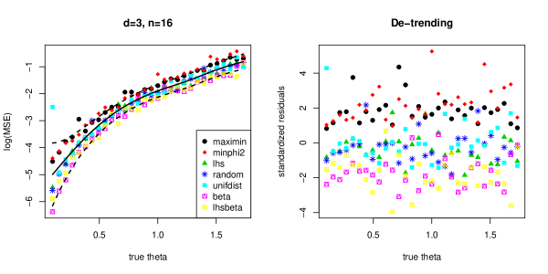
Figure 1: logMSEs from design experiment and de-trending surface.

As an example of the logMSEs obtained, the left panel of Figure 1 shows the $(d=3,n=16)$ case. The first thing to notice in that plot is that as $\theta^{(t)}$ increases so does $\mathrm{logMSE}_{t}$, for all design methods. Apparently, it is “harder” to accurately estimate lengthscales $\theta$ as they become longer. Harder is in quotes because this metric obscures the relative performance of the design methods, although some consistently stand out as worse (maximin/black circles) or better (beta/pink squares or lhsbeta/yellow squares) than others. To level the playing field for subsequent analysis, we calculated standardized residuals using a de-trending surface estimated from all of the dots, taken together. To cope with the outliers we fit a heteroskedastic Student-$t$ GP as described by Chung et al., (2018) and implemented in the hetGP package (Binois and Gramacy,, 2018). Section 3.2 provides further details on our use of hetGP in this context. Standardized residuals ($r_{t}=(\mathrm{logMSE}_{t}-\mu_{t})/\sigma_{t}$, with $\mu_{t}$ and $\sigma_{t}$ from hetGP), are shown in the right panel of the figure.

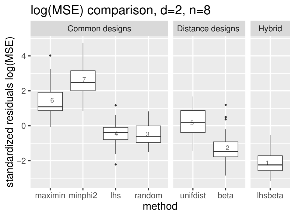
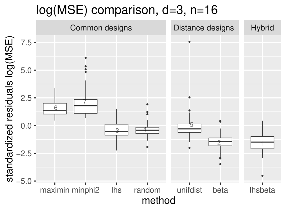
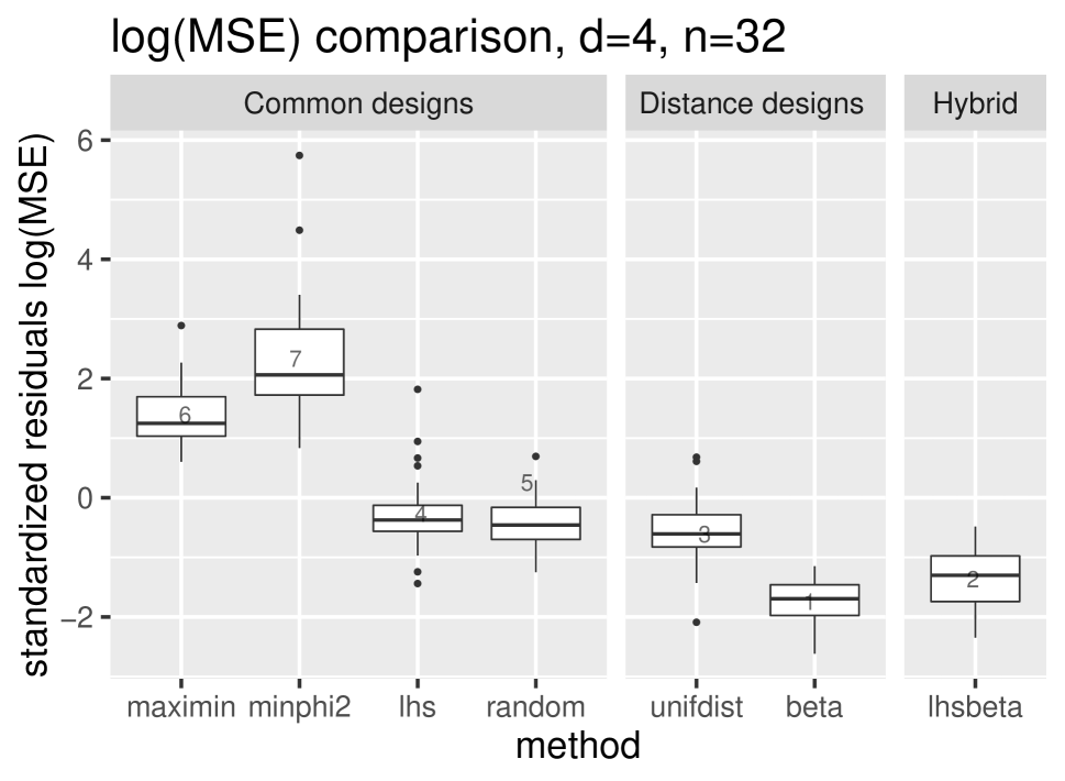
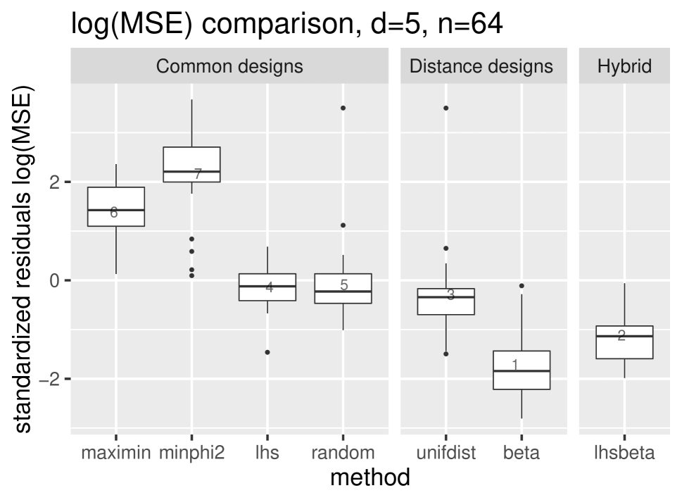
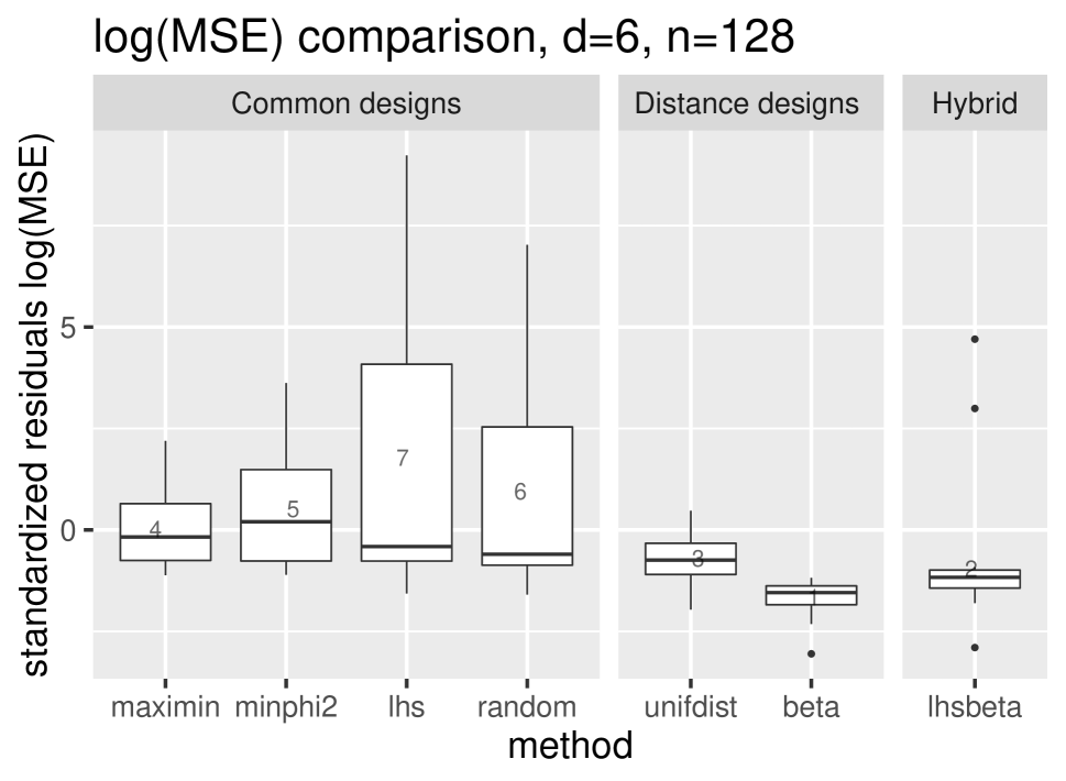
rank	2d	3d	4d	5d	6d
2	9.78e-4	0.406	2.58e-4	2.90e-5	5.58e-3
3	1.29e-4	7.92e-8	1.16e-7	4.61e-7	0.213
4	0.388	0.151	7.14e-3	0.134	9.03e-8
5	3.02e-3	0.287	0.415	0.446	6.64e-5
6	2.06e-5	1.08e-7	5.35e-4	3.51e-9	0.261
7	1.08e-5	0.0410	4.72e-6	1.06e-6	0.123

Figure 2: Standardized logMSE boxplots to thirty gridded $\theta^{(t)}$ values for seven comparators using $n=2^{d+1}$ over input dimension $d\in\{2,3,4,5,6\}$. The comparators are described in the text. Two outlying standardized $\log\mathrm{MSE}$ values were clipped by the $y$-axes to enhance boxplot viewing: random ($d=4$) at 10.9 and LHS ($d=6$) at 17.4. The bottom-right panel provides $p$-values for lower-tail paired $t$-tests comparing adjacent performers as ranked by their mean logMSE from best (top) to worst (bottom).

Figure 2 shows boxplots of these standardized logMSEs, marginalizing over $\theta^{(t)}$s, for all five experiments $d\in\{2,3,4,5,6\}$. The number written on each boxplot resides in the position of the mean of that comparator, and indicates relative rank of that mean. In order to help better quantify relative comparisons, the final panel provides the outcome of pairwise paired $t$-tests, with pairing determined by adjacent ranks: best vs. second best, etc. First consider the “Common designs” block including boxplots of logMSEs for maximin, minphi2 ($\phi_{2}$), LHS and random designs. Although the final panel does not include a $p$-value for LHS or random vs. maximin when $d$ = 2,3, because neither is ranked adjacently with maximin, it is quite clear these beat maximin, which consistently beats minphi2. LHS and random, on the other hand, offer quite similar results.

Observe that the four “Common designs” follow a similar ranking for all $d\leq 5$. However when $d=6$ maximin and minphi2 are better than LHS and random. This happens because maximin’s (and $\phi_{p}$’s) pathologies are partly corrected in higher dimension. These designs push sites to the corners of the input hyperrectangle. As dimension grows the diversity of distances between corners increases. This helps MSE, but only coincidentally. Deliberate diversity via unifdist and betadist is still better.

The outcome of this experiment, including just those four common designs as comparators, sparked our search for alternatives. It is perhaps surprising that a purely random design is at least as good for hyperparameter estimation as more thoughtful alternatives like maximin and LHS. The following subsections describe our journey towards improved designs, ultimately outlining details behind the other comparators in Figure 2.

3.1 Uniform to beta designs

Intuitively, random and LHS are better than maximin for lengthscale ($\theta$) inference because they result in a less adversarial distribution of pairwise distances. Maximin designs are calculated to ensure there are no small pairwise distances, which is presumably too few. Consequently, the distance distribution is multimodal: there are many distances near that minimum, with the rest occurring at “lower harmonics” (multiples of that minimal distance). Figure 3 offers a visualization. Random and LHS designs do not preclude small relative distances, although the latter does enforce a degree of uniformity in position. Both tend to yield distance distributions which are unimodal. Figure 3 demonstrates this for a subset of random designs, which will be discussed in more detail momentarily. The situation is similar for LHS, which we shall revisit in Section 4.

Init: Fill $\mathbf{X}$ with a random design of size $n$, i.e, $\mathbf{x}_{i}\stackrel{{\scriptstyle\mathrm{iid}}}{{\sim}}\mathrm{Unif}[0,1]^{d}$, $i=1,\dots,n$.

for $s=1,\dots,S$ do

       Select an index $i\in\{1,\dots,n\}$ at random.

       Generate $\mathbf{x}_{i}^{\prime}\sim\mathrm{Unif[0,1]}^{d}$.

       Propose new design $\mathbf{X}^{\prime}$ as $\mathbf{X}$ with $\mathbf{x}_{i}$ swapped with $\mathbf{x}_{i}^{\prime}$.

       if $\mathrm{KSD}(\mathbf{X}^{\prime},F)<\mathrm{KSD}(\mathbf{X},F)$  then

             $\mathbf{x}_{i}\leftarrow\mathbf{x}_{i}^{\prime}$ in the $i^{\mathrm{th}}$ row of $\mathbf{X}$;

             i.e., accept $\mathbf{X}\leftarrow\mathbf{X}^{\prime}$

       end if

      

end for

Return: $n\times d$ design $\mathbf{X}$.

Algorithm 1 MC calculation of size $n$ in $[0,1]^{d}$ targeting distance distribution $F$.

The experimental outcomes just described got us thinking about desirable distance distributions for lengthscale estimation. We speculated that it could be advantageous to have a uniform distance design (unifdist), so that all distances were represented—or as many as possible up to the desired design size $n$. Throughout we presume inputs have been scaled to $[0,1]^{d}$, and restrict the search for lengthscales to $\theta\in(0,\sqrt{d}]$. So when we say uniform, or any other distribution, we mean $\mathrm{Unif}(0,\sqrt{d}]$. To calculate a design whose distribution of pairwise distances resembles a reference $F$, we follow the pseudo-code provided by Algorithm 1 which is based on $S$ stochastic swap proposals that are accepted or rejected via Kolmogorov-Smirnov distances (KSD) against $F$. In our examples we fix $S=10^{5}$ and utilize a faster, custom implementation of KSD based on isolating the $statistic output of the built-in ks.test function in R. Besides being stochastic, the search is greedy which means that it only guarantees local convergence as $S\rightarrow\infty$. Nevertheless we find that in practice it furnishes empirical pairwise distance distributions close to the target $F$. There is little benefit in restarting the algorithm to search for a more global optimum.

Unfortunately, our intuition about unifdist designs didn’t completely match our results. As summarized along with our earlier RMSE comparison in Figure 2, unifdist designs are better than maximin, but worse than LHS and random. This outcome prompted a more careful investigation into why random designs, work so well.

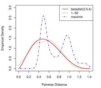
Figure 3: Empirical density curves corresponding to random designs in 2d with lowest 50 logMSE($\theta$) values from 1000 random design realizations. Empirical maximin and $\mathrm{Beta}(2.5,4)$ densities are shown for comparison.

Consider the lines in Figure 3 labeled “1–50”, representing the empirical density of distances among the random designs whose logMSE was among the fifty best in a large Monte Carlo (MC) exercise. Observe that this density is unimodal, having more small distances than maximin and very few really large distances. The solid red curve in the figure is a $\mathrm{Beta}(2.5,4)$ density scaled to $[0,\sqrt{2}]$ as a representative example of a parametric distribution similar to that of those best random distances.

Unifdist designs, which are not shown in the figure, target a flat line across the $[0,\sqrt{2}]$ domain. Unifdist outperforms maximin, but not the best (or even the typical) random designs. This suggests that while having more short distances is desirable, having as many distances at the extremes—both large and small—may not be helpful on average. As the results in Figure 2 show, having Beta-distributed distances, focusing the distribution on mid–low-range pairwise distances, leads to statistically significant improvements over random in all three cases. In fact, these “betadist” designs (being ranked 2 or 1) are the only ones in that figure whose logMSEs are statistically better (see $p$-values in the lower-right panel) than all other designs of lower rank.

Although Figure 3 suggests that a $\mathrm{Beta}(2.5,4)$ is a good target distribution for a betadist design, that was not the specification used to generate all results summarized in Figure 2. The best setting of shape parameters, $(\hat{\alpha},\hat{\beta})$ in $\mathrm{Beta}(\alpha,\beta)$ depends on dimension $d$ and design size $n$, as we explore below. However, it is worth nothing that $\mathrm{Beta}(2.5,4)$ does generally perform well because, as we show, the set of decent $(\alpha,\beta)$ values is relatively big, and does not vary substantially in $n$ and $d$. But it’s not so big as to choose arbitrarily.

3.2 Optimization of shape parameters of betadist design

Here we view the choice of betadist parameterization, $\hat{\alpha}$ and $\hat{\beta}$ in $\mathrm{Beta}(\alpha,\beta)$, for particular design size $n$ in input dimension $d$, as an optimization problem. I.e., we wish to automate the search for $\mathrm{betadist}_{n,d}(\hat{\alpha},\hat{\beta})$. Discussion around Figure 1 indicates that a degree of detrending will be required in order to not over-emphasize larger $\theta$ settings in the optimization criteria. To address this, we seek $(\hat{\alpha},\hat{\beta})=\mathrm{argmin}_{\alpha,\beta}\;\mathrm{deRIMSE}_{n,d}(\alpha,\beta)$ where the criteria deRIMSE is defined following a scheme similar to that described around Figure 1.

Begin by establishing a regular grid of $\theta$ values $(\theta^{(1)}=0.1,\dots,\theta^{(T)}=\sqrt{d})$, just like in Figure 1. Next, generate one pair $(\alpha,\beta)\sim\mathrm{Unif}(1,10)^{2}$ and use these to create $D$ designs $\mathbf{X}_{n}^{(i)}\sim\mathrm{betadist}_{n,d}(\alpha,\beta)$, for $i=1,\dots,D$ following Algorithm 1. Averaging over more random $(\alpha,\beta)$ will be described momentarily. For each $\mathbf{X}_{n}^{(i)}$ and each $\theta^{(t)}$ generate random responses $\mathbf{Y}_{n}^{(t,i)}\sim(\mathbf{X}_{n}^{(i)},\theta^{(t)})$ under the GP MVN and estimate $\hat{\theta}^{(t,i)}$ via MLE. Finally, calculate $\mathrm{RMSE}^{(t)}=\sqrt{\sum_{i=1}^{D}(\hat{\theta}^{(t,i)}-\theta^{(t)})^{2}/D}$ to estimate the accuracy of those MLE calculations for each $t=1,\dots,T$. Then draw new $(\alpha,\beta)\sim\mathrm{Unif}(1,10)^{2}$ yielding $\mathrm{RMSE}^{(t,r)}$, repeating the entire scheme above $R$ times, i.e., for $r=1,\dots,R$. In our empirical work, we chose $D=5$ and $R=T=30$.

Next, take pairs $(\theta^{(t)},\{\mathrm{RMSE}^{(t,r)}\}_{r=1}^{R})$ as $T\times R$ observations of the quality of lengthscale estimation – RMSE dynamics – across $\theta$-space and fit a Student-$t$ hetGP to these observations yielding a surrogate described by mean $\mu_{t}\equiv\mu(\theta^{(t)})$ and $\sigma^{2}_{t}\equiv\sigma^{2}(\theta^{(t)})$. Now we are ready to define the criteria $\mathrm{deRIMSE}_{n,d}(\alpha,\beta)$ as

$$\mathrm{deRIMSE}(\alpha,\beta)\equiv\frac{1}{T}\sum_{t=1}^{T}\frac{\mathrm{RMSE}^{(t)}(\alpha,\beta)-\mu_{t}}{\sigma_{t}},$$

where $\mathrm{RMSE}^{(t)}(\alpha,\beta)$ is calculated just as described above with the specific (not random) settings of $(\alpha,\beta)$ in question.

As a warmup experiment toward solving that optimization problem, consider $n=16$ and $d=2$. We built a size 200 LHS design of $(\alpha,\beta)$ settings in $[1,10]^{2}$ with 5 replicates on each for a total of 1000 evaluations of $\mathrm{deRIMSE}$. The bottom end of that region, $\alpha,\beta\geq 1$, was chosen to limit the search to unimodal beta distributions; the top end of 10 was chosen based on a smaller pilot study. Each deRIMSE evaluation took about 50 seconds, leading to almost 14 hours of total simulation time.

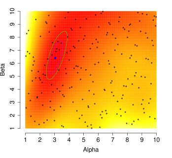
Figure 4: deRIMSE surface with $T=1000$ for $n=16$ and $d=2$ as estimated by hetGP. Dots show the design sites; lighter (heat) colors correspond to higher deRIMSEs.

Figure 4 shows the design (dots) and fitted surface of deRIMSE values obtained with hetGP, i.e., treating $\mathrm{deRIMSE}$ simulation as a stochastic computer experiment and fitting a surrogate to a limited number of evaluations. Outliers are less of a concern when averaging over $\theta^{(t)}$-values, so there was no need to include Student-$t$ features in this regression. However, accommodating a degree of heteroskedasticity and leveraging replication in the calculations were essential to obtain a good fit in a reasonable amount of time (Binois et al.,, 2018a). The blue square, at about $(\hat{\alpha},\hat{\beta})=(3,6.5)$ in the figure, shows where the predictive surface is minimized; the green and purple contours outline regions wherein predicted deRIMSE values are within 5% and 10% of that best setting.

Fourteen hours of simulation in order to choose the characteristics of a random design is rather extreme. However, once done for a particular choice of covariance structure, design size $n$ and dimension $d$, it need not be re-done. Still, finding appropriate designs in higher dimension, with more runs to fill out the larger volume could be computationally daunting. Doubling $n$, for example, would result in more than double the computational effort.

For a more thrifty approach we turn to BO via EI. The idea is to replace a space-filling evaluation with a sequential design strategy that targets the minimum of the mean of $\mathrm{deRIMSE}$. For a given $(n,d)$-setting, the setup is as follows. Begin by performing deRIMSE calculations on a maximin design of size twenty, with ten replicates at each setting, and by fitting a hetGP to those realizations, deriving a predictive surface. Then comes the so-called BO acquisition. Based on hetGP posterior predictive equations described by mean $\mu(\mathbf{x})$ and standard deviation $\sigma(\mathbf{x})$, where $\mathbf{x}=(\alpha,\beta)$ in this case, numerically optimize $\mathrm{EI}(\mathbf{x})$:

$$\mathrm{EI}(\mathbf{x})=(\mu_{\min}-\mu(\mathbf{x}))\Phi\left(\frac{\mu_{\min}-\mu(\mathbf{x})}{\sigma(\mathbf{x})}\right)+\sigma(\mathbf{x})\phi\left(\frac{\mu_{\min}-\mu(\mathbf{x})}{\sigma(\mathbf{x})}\right),$$ (3)

where $\mu_{\min}=\min_{\mathbf{x}}\mu(\mathbf{x})$ and $\Phi$ and $\phi$ are the standard Gaussian cdf and pdf, respectively. After (a) solving $\mathbf{x}^{*}=\mathrm{argmin}_{\mathbf{x}}\;\mathrm{EI}(\mathbf{x})$, which we accomplish using a hybrid of discrete search over replicates and continuous multi-start R–optim-based search with method="L-BFGS-B"; (b) simulating $y^{*}=\mathrm{deRIMSE}(\mathbf{x}^{*})$; and (c) incorporating the new data pair into the design and updating the hetGP model fit; the process repeats (back to (a)).

For details on EI and BO see Jones et al., (1998) and Chapter 6.3 of Santner et al., (2003). Snoek et al., (2012) offer a somewhat more modern machine learning perspective centered around the use of BO for estimating hyperparameters of deep neural networks. Our use here—to tune a design—is related in spirit but distinct in form. In fact, the setup we propose is fractal. It solves a design problem (for estimating lengthscale) with the solution to another design problem: for function minimization. One could argue that our choice of an initial maximin design for BO is sub-optimal, and we will do just that in Section 5.2.

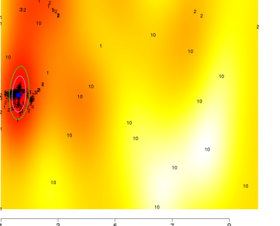
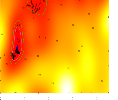
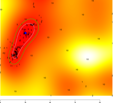
$n=8$, $d=2$	$n=16$, $d=2$	$n=16$, $d=3$
$\hat{\alpha}=1.62$, $\hat{\beta}=5.26$	$\hat{\alpha}=2.4$, $\hat{\beta}=5$	$\hat{\alpha}=3.02$, $\hat{\beta}=6.38$
$\tilde{\alpha}=1.5$, $\tilde{\beta}=5$	$\tilde{\alpha}=2$, $\tilde{\beta}=4$	$\hat{\alpha}=2.5$, $\tilde{\beta}=5$
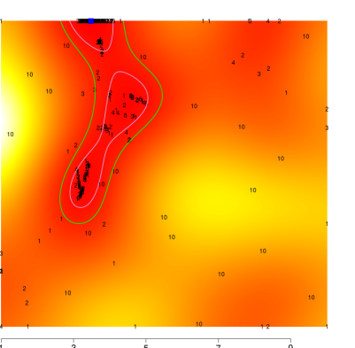
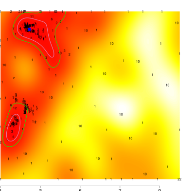
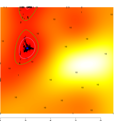
$n=32$, $d=3$	$n=32$, $d=4$	$n=64$, $d=4$
$\hat{\alpha}=3.48$, $\hat{\beta}=10$	$\hat{\alpha}=2.44$, $\hat{\beta}=9.06$	$\hat{\alpha}=3.15$, $\hat{\beta}=6.53$
$\tilde{\alpha}=3$, $\tilde{\beta}=5$	$\tilde{\alpha}=1.5$, $\tilde{\beta}=3.5$	$\hat{\alpha}=3$, $\tilde{\beta}=6$
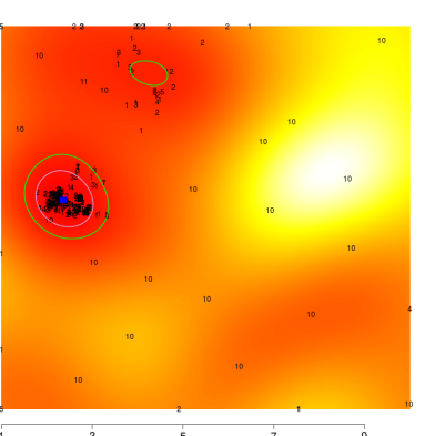
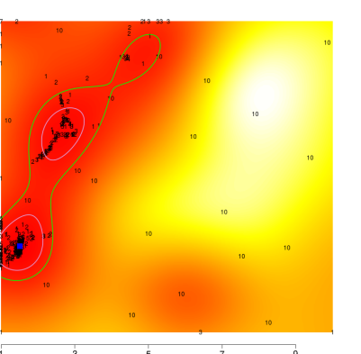
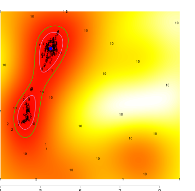
$n=64$, $d=5$	$n=128$, $d=5$	$n=128$, $d=6$
$\hat{\alpha}=2.36$, $\hat{\beta}=5.92$	$\hat{\alpha}=1.51$, $\hat{\beta}=3.5$	$\hat{\alpha}=3.52$, $\hat{\beta}=8.01$
$\tilde{\alpha}=2$, $\tilde{\beta}=6$	$\tilde{\alpha}=1$, $\tilde{\beta}=3$	$\hat{\alpha}=2$, $\tilde{\beta}=4$

Figure 5: Outcomes of BO of RIMSE surfaces for various choices of $n$ and $d$. Numbers show location and number of replicates in acquisitions; blue square shows $(\hat{\alpha},\hat{\beta})$; purple and green contours show 5% and 10% from the optimal.

For a set of representative $n$ and $d$, we allowed our BO scheme to collect an additional $600$ deRIMSE simulations. The resulting selections, overlayed with final predictive mean surface from hetGP, the best value of $(\hat{\alpha},\hat{\beta})$ and a 5% and 10% contour are shown in Figure 5. Several noteworthy patterns emerge from the panels in the figure. First, although some of the surfaces appear to be multimodal, or at least to have ridges of low deRIMSE values, there is usually a setting with relatively low $(\alpha,\beta)$ which works well. Sometimes a larger setting is predicted as optimal; but there is usually an alternate setting, reported as $(\tilde{\alpha},\tilde{\beta})$ in the figure, which is almost as good (within 5%).

These “near-optimal” $(\tilde{\alpha},\tilde{\beta})$ were used in our betadist designs, and subsequent boxplots and $p$-value calculations, in Figure 1. They are re-used throughout the remainder of the paper in our empirical work [Sections 5.1–5.2], and likewise with the hybrid lhsbeta designs discussed momentarily. Although the computational demands are still sizable even with the more thrifty BO, these designs are “up-front”. Once saved as we do for the nine choices above, no recalculation is required.

4 Hybrid betadist and LHS

Having a betadist design, which provides better estimates of hyperparameters like the lengthscale $\theta$, is advantageous only insofar as the resulting surrogate fits, i.e., their predictive equations (2), are accurate. Since GP surrogates are inherently spatial predictors, practitioners have long preferred designs which fill the space, so that those sites may serve as nearby anchors to good out-of-sample predictive performance. Betadist designs space-fill less than common alternatives, both quantitatively (i.e., via the maximin criteria) and qualitatively (since they’re inherently random). Thus they hold the potential to be inferior as predictive anchors. Yet in our empirical work, we’ve only been able to demonstrate this negative result (not shown here) when good hyperparameter settings are known. Betadist shines brightest in sequential application [Section 5], where the impact of early estimates of hyperparameters can have a substantial affect—exceptionally deleterious in pathological cases—on subsequent design decisions in several common situations.

Still, betadist designs consider only relative distance, completely ignoring position except that the points lie in the study area. Among more-or-less equivalent optimal betadist designs, some may have better positional properties and thus offer better anchoring for prediction without compromising on hyperparameter quality. To explore this possibility we considered a hybrid between betadist and LHS designs. Our “lhsbeta” is similar in spirit to maximin–LHS hybrids where maximin helps avoid second-order aliasing common with LHSs, and LHS helps maximin avoid clumpy marginals. In lhsbeta, we primarily view LHS as helping betadist acquire a degree of positional preference, however the alternate perspective of preferring LHSs with better relative distances is no less valid.

Our stochastic search strategy for finding lhsbeta designs is coded in Algorithm 2.

Init: Fill $\mathbf{X}$ with a LHS of size $n$ in $d$ dimensions.

for $s=1,\dots,S$ do

       Randomly select a pair of design points $\mathbf{x}_{i},\mathbf{x}_{j}$.

       Randomly select a dimension $k\in\{1,\dots,d\}$.

       Propose a new design $\mathbf{X}^{\prime}$ by swapping Latin squares $L_{i,k}$ and $L_{j,k}$ producing

         new $\mathbf{x}_{i}^{\prime}$ and $\mathbf{x}_{j}^{\prime}$ after re-jittering with $2d$ new uniform random numbers.

       if $\mathrm{KSD}(\mathbf{X}^{\prime},F)<\mathrm{KSD}(\mathbf{X},F)$  then

             $\mathbf{x}_{i}\leftarrow\mathbf{x}_{i}^{\prime}$ and $\mathbf{x}_{j}\leftarrow\mathbf{x}_{j}^{\prime}$ in the $(i,j)^{\mathrm{th}}$ rows of $\mathbf{X}$;

             i.e., accept $\mathbf{X}\leftarrow\mathbf{X}^{\prime}$

       end if

      

end for

Algorithm 2 Hybrid $F$-dist–LHS via $S$ MC iterations for a design of size $n$ in $d$ dimensions.

Like in Algorithm 1 for betadist, we presume an input space coded to $[0,1]^{d}$. The algorithm is initialized with an LHS $\mathbf{X}$, built in the canonical way (see, e.g., Lin and Tang,, 2015) by first choosing $d$ random permutations of $\{1,\dots,n\}$, saved in a $n\times d$ matrix $\mathbf{L}$ describing the $n$ selected hypercubes out of the $n^{d}$ possible partitions of the input space, and then applying jitter in that selected cube. Each subsequent iteration of stochastic search involves randomly proposing to swap pairs of rows and columns of $\mathbf{L}$, effectively swapping the pair of Latin squares without destroying the one-dimensional uniformity property, and then rejittering that pair points within their respective squares. That proposal is then accepted or rejected according to KSD measured against a distribution $F$, which in our applications is $\mathrm{Beta}(\tilde{\alpha},\tilde{\beta})$ from Section 3. Since two types of random proposals are being performed simultaneously, compared to Algorithm 1’s single random swap, we prefer a multiple of two larger $S$ in Algorithm 2; $S=10^{5}$ in our empirical work.

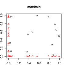
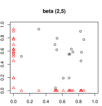
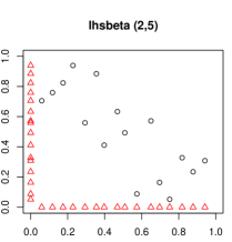
Figure 6: 2d (black circles) and 1d (red triangles) projections of three $d=3$ designs, $n=16$.

Figure 6 shows a visual comparison between maximin, betadist and lhsbeta designs so constructed. The plots provide a 2d projection for the case $n=16$ and $d=3$. Observe that maximin’s 1d margins, shown as red triangles at the axes in the left panel, are not uniform. Neither are those in the 2d projection shown as open circles. First-order aliasing is severe in both projections. In the middle panel, our betadist design has a similar problem (although perhaps not to the same degree), yet we know that the distribution of pairwise distances in 3d are much better than maximin for the purpose of lengthscale inference. In the right panel the 1d and 2d margins look much better, because the sample is an LHS. Among LHSs, this lhsbeta design has a near optimal distribution of pairwise distances for this setting $(n,d)$. Figure 2 shows that lhsbeta designs are sometimes worse than ordinary betadist designs, but they both are consistently better than all of the other comparators in the figure. This is perhaps not surprising because lhsbeta designs are indeed betadist designs, yet selected for an additional feature not relevant for lengthscale information: space-fillingness. As we show in two prediction-based comparisons below, lhsbeta designs are sometimes superior on those tasks.

5 Application to sequential design

Here we provide two applications of betadist and lhsdist as initial designs for a subsequent sequential analysis. In both cases, these distance distribution-based designs are only engaged in a limited way, as a means of seeding the sequential procedure. Subsequent design acquisitions are then off-loaded to other criteria. Still, it is remarkable how profound the effect of this initial choice can be. A poorly chosen initial design of just $n_{\mathrm{init}}=8$ points, say, can be detrimental to predictive accuracy at $n=64$.

5.1 Active Learning MacKay

First consider the so-called active learning MacKay (ALM; MacKay,, 1992) method of sequential design for reducing predictive uncertainty. Acquisitions are determined by maximizing the predictive variance $\sigma^{2}(\mathbf{x})$. The rationale for that choice is that ME designs for GPs involve maximizing the determinant of the covariance matrix $\mathbf{K}_{n}$, and one can show that $\log|\mathbf{K}_{n+1}|=\log|\mathbf{K}_{n}|+\log\sigma^{2}(\mathbf{x}_{n+1})$. After many applications the result is space-filling, however the degree to which design points are pushed toward the boundaries of the study region depends crucially on the lengthscale(s) used to define $\mathbf{K}_{n}$. For more details on ALM with GPs see, e.g., Seo et al., (2000) and Gramacy and Lee, (2009).

The target of our experiment is a function $f(\mathbf{x})$ observed under light noise as $Y(\mathbf{x})=f(\mathbf{x})+\varepsilon$, with $\varepsilon\stackrel{{\scriptstyle\mathrm{iid}}}{{\sim}}\mathcal{N}(0,0.01^{2})$. For $f(\mathbf{x})$ we use the function

$$f(\mathbf{x})=x_{1}\exp\{-x_{i}^{2}-x_{2}^{2}\}\quad\mbox{ with }\mathbf{x}\in[-2,4]^{2},$$

first introduced as an active learning benchmark by Gramacy and Lee, (2009). We begin with an initial design of size $n_{\mathrm{init}}=8$, and perform 56 additional ALM acquisitions for a total of $n=64$ evaluations. Along the way, root mean-squared prediction error (RMSPE) is calculated on noise-free outputs obtained on a regular $100\times 100$ testing grid in the input space. For the initial design, we consider random, LHS, 2d optimal $(\tilde{\alpha}=2,\tilde{\beta}=5)$ betadist and lhsdist designs, and maximin. Unifdist has been dropped from the comparison on the grounds that it is a sub-optimal betadist alternative.

In keeping with our earlier experiments, MLE calculations limited to $(0,\sqrt{2}]$ are updated after each sequential design acquisition. To accommodate the noisy evaluations, we augment our covariance with a nugget hyperparameter which is included in the MLE calculation via jmleGP in the laGP package. An L-BFGS-B scheme is used to solve $\mathrm{argmin}_{\mathbf{x}}\sigma^{2}(\mathbf{x})$ via optim in R. Variance surfaces can be highly multi-modal, having as many maxima as design points which is what creates the “sausage”-like shape characteristic of the error-bars produced by GP predictive equations. We deployed an $n$-factor sequential maximin multi-start scheme to avoid inferior local modes of the variance surface. This means that maximin is used to choose the optim initializations, in order to space out starting locations relative to each other and to the existing $X_{n}$ design locations.

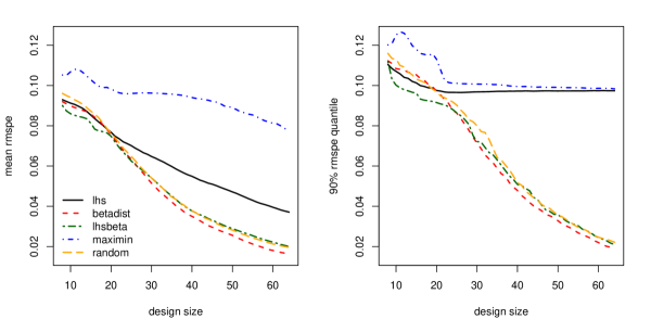
Figure 7: RMSPE comparison of initial designs ($n_{\mathrm{init}}=8$) as a function of the number of subsequent sequential design iterations via ALM. Each comparator has a pair of lines: those in the left panel indicate mean RMSE; those on the right are the upper 90% quantile.

Figure 7 shows the outcome of this exercise via mean RMSPE (left panel) and upper 90% RMSPE quantile (right) obtained from 1000 MC repetitions of the scheme described above. Several striking observations stand out. Betadist, lhsbeta and random perform about the same, with betadist winning out in the end. However in early stages lhsdist is best and random is the worst of the three. Beta-distributed distances (from betadist and lhsbeta) lead to better hyperparameter estimates than random. Yet position of design sites is more important than lengthscale quality when there are little data. After many sequential acquisitions, position is less important—ALM takes care of that—but the final results are still sensitive to the choice of the first $n_{\mathrm{init}}=8$ points, even though MLEs $\hat{\theta}$ are recalculated after each selection. Seeding the sequential design, which is often glossed over as an implementation detail, can be crucial to good performance in active learning.

Consequently, betadist, lhsbeta and random vastly outperform LHS and maximin. The trouble with these space-filling seed designs is evident in the 90% quantile, which fails to improve even after many new design sites are added. Too much spread in the initial design results in large $\hat{\theta}$s, which is reinforced by subsequent ALM acquisitions at the boundaries of the input space. The early behavior of maximin is particularly strange: getting worse before better even in cases where sequential acquisitions lead to decent results. It’s 90% quantile is eventually no worse than LHS’s—quite poor. The fact that maximin’s average RMSPE is nearly as bad suggests that maximin rarely recovers from that poor initial design.

5.2 Expected improvement for optimization

Here we show that betadist and lhsbeta initial designs are also superior in a BO context similar to that used to find the best $\hat{\alpha}$ and $\hat{\beta}$ settings in Section 3.2. Specifically, acquisitions are gathered via EI (3) using a random five-start scheme including the location of the best input setting (corresponding to $\mu_{\min}$) from the previous iteration. As a test function, we use the so-called Greiwank function

$$f_{d}(\mathbf{x})=\sum_{i=1}^{d}\frac{x_{i}^{2}}{4000}-\prod_{i=1}^{d}\cos\left(\frac{x_{i}}{\sqrt{i}}\right)+1.$$

For visualizations and further details, including R implementation, see the Virtual Library of Simulation Experiments: https://www.sfu.ca/~ssurjano/griewank.html.

A nice feature of the Greiwank is that it is defined for arbitrary input dimension $d$, and is flexible about the bounds $b$ of the inputs, $\mathbf{x}\in[-b,b]^{d}$. These two settings, $b$ and $d$, together determine the complexity of the response surface. The global minima is always at the origin, however the number of local minima grows quickly as $b$ and $d$ are increased. We utilize these knobs to vary the complexity of the function, in order to span a range of optimization problems. By varying the bounds $b$ in particular, we vary the magnitude of the best lengthscale for the purpose of surrogate modeling, and thereby create a situation where an initial design is key to obtaining good performance in BO.

Our experimental setup is as follows. We consider three $(n_{\mathrm{init}},d)$-pairs from Figure 5 and track the progress of EI-based BO measured by the lowest value of the objective found over the sequential design iterations. In each of one thousand MC repetitions, we create initial $n_{\mathrm{init}}$-sized designs via maximin, random, LHS, betadist and lhsbeta, with subsequent acquisitions handled by EI. In accordance with the theory for convergence of EI-based BO (Bull,, 2011), we do not update $\hat{\theta}$ after each EI acquisition, but fix it at the setting obtained immediately after the initial design. This has the benefit of accentuating the effect of the initial design, which suits our illustrative purposes. It is also more computationally efficient, leading to an $O(n^{3})$ calculation rather than $O(n^{4})$ if MLEs are recalculated regularly. However the results are not much different under that latter alternative.

To vary the complexity of the underlying optimization problem, and thus best effective lengthscale for GP surrogate, we draw $b\sim\mathrm{Unif}(0,10)$ at the start of each MC repetition. In so doing, each of 1000 MC repetitions targets a Greiwank function having a different degree of waviness, and number of local optima. By holding $b$ fixed for each of the five initial design choices, and subsequent EI-optimizations, we create a setting wherein pairwise $t$-tests can be used to adjudicate between those comparators. Finally, all calculations were formed with methods built into the laGP package on CRAN. Since we observe $f_{d}(\mathbf{x})$ without noise, no nugget hyperparameters are required. Not presuming to know the randomly generated scale $b$, we allow MLE calculations for $\hat{\theta}$ to search in a space that would be appropriate for the largest settings, $\theta\in(0,10\sqrt{d}]$, regardless of $b$.

$n=25$	maximin	LHS	random	betadist	lhsbeta
maximin	NA	0.95	0.98	$>$ 0.99	$>$ 0.99
LHS	0.048	NA	0.67	$>$ 0.99	$>$ 0.99
random	0.022	0.33	NA	$>$ 0.99	$>$ 0.99
betadist	$<$ 1e-7	2e-5	8e-5	NA	$>$ 0.99
lhsbeta	$<$ 1e-7	$<$ 1e-7	$<$ 1e-7	$<$ 1e-7	NA

$n=70$	maximin	LHS	random	betadist	lhsbeta
maximin	NA	$>$ 0.99	$>$ 0.99	$>$ 0.99	$>$ 0.99
LHS	5e-7	NA	0.89	$>$ 0.99	$>$ 0.99
random	$<$ 1e-7	0.11	NA	$>$ 0.99	$>$ 0.99
betadist	$<$ 1e-7	$<$ 1e-7	2e-6	NA	$>$ 0.99
lhsbeta	$<$ 1e-7	$<$ 1e-7	$<$ 1e-7	$<$ 1e-7	NA

Table 1: Pairwise $t$-test $p$-value table for $(n_{\mathrm{init}}=8,d=2)$ and two settings $n=25$ (top table) and $n=70$ (bottom). Statistically significant $p$-values, i.e., below 5%, are in bold.

Table 1 summarizes results obtained from the ($n_{\mathrm{init}}=8$, $d=2$) case in two views: after $n=20$ total acquisitions, and then after $n=70$. The bolded $p$-values in the table(s) are below the typical 5% threshold. Observe in both cases that random and LHS design are consistently better than maximin, but betadist is significantly better than all three. Hybrid lhsbeta outperforms all of the others. In other words, the story here is more or less the same as before. The only substantial difference is that lhsbeta outperforms betadist.

$n=50$	maximin	LHS	random	betadist	lhsbeta
maximin	NA	$>$ 0.99	$>$ 0.99	$>$ 0.99	$>$ 0.99
LHS	$<$ 1e-7	NA	0.95	$>$ 0.99	$>$ 0.99
random	$<$ 1e-7	5.3e-2	NA	$>$ 0.99	$>$ 0.99
betadist	$<$ 1e-7	$<$ 1e-7	$<$ 1e-7	NA	$>$ 0.99
lhsbeta	$<$ 1e-7	$<$ 1e-7	$<$ 1e-7	1e-3	NA

$n=100$	maximin	LHS	random	betadist	lhsbeta
maximin	NA	$>$ 0.99	$>$ 0.99	$>$ 0.99	$>$ 0.99
LHS	$<$1e-7	NA	$>$ 0.99	$>$ 0.99	$>$ 0.99
random	$<$ 1e-7	3e-3	NA	$>$ 0.99	$>$ 0.99
betadist	$<$ 1e-7	$<$ 1e-7	$<$ 1e-7	NA	$>$ 0.99
lhsbeta	$<$ 1e-7	$<$ 1e-7	$<$ 1e-7	8e-3	NA

Table 2: Pairwise $t$-test $p$-value table for $(n_{\mathrm{init}}=16,d=3)$ and two settings $n=50$ (top table) and $n=100$ (bottom). Statistically significant $p$-values, i.e., below 5%, are in bold.

Table 2 summarizes results from the $(n_{\mathrm{init}}=16,d=3)$ case. In higher dimension, the problem is more challenging with many more local minima. Both a bigger initial design, and a larger run of EI acquisitions is necessary in order to obtain reliable results. At $n=50$ the pecking order is similar: maximin, LHS, betadist, lhsbeta—all statistically significant at the 5% level. Random outperforms LHS, but not significantly so at the 5% level.

$n=200$	maximin	LHS	random	betadist	lhsbeta
maximin	NA	$>$ 0.99	$>$ 0.99	$>$ 0.99	$>$ 0.99
LHS	$<$ 1e-7	NA	0.43	$>$ 0.99	$>$ 0.99
random	$<$ 1e-7	0.57	NA	$>$ 0.99	$>$ 0.99
betadist	$<$ 1e-7	2e-4	2e-4	NA	$>$ 0.99
lhsbeta	$<$ 1e-7	$<$ 1e-7	$<$ 1e-7	$<$1e-7	NA

$n=500$	maximin	LHS	random	betadist	lhsbeta
maximin	NA	$>$ 0.99	$>$ 0.99	$>$ 0.99	$>$ 0.99
LHS	$<$1e-7	NA	0.25	$>$ 0.99	$>$ 0.99
random	$<$ 1e-7	0.75	NA	$>$ 0.99	$>$ 0.99
betadist	$<$ 1e-7	8e-3	2e-3	NA	$>$ 0.99
lhsbeta	$<$ 1e-7	$<$ 1e-7	$<$ 1e-7	$<$ 1e-7	NA

Table 3: Pairwise $t$-test $p$-value table for $(n_{\mathrm{init}}=32,d=4)$ and two settings $n=200$ (top table) and $n=500$ (bottom). Statistically significant $p$-values, i.e., below 5%, are in bold.

Finally, Table 3 summarizes the $(n_{\mathrm{init}}=32,d=4)$ case with $n=200$ and $n=500$. Except when the randomly chosen $b$ is very small, this setting represents an extremely difficult optimization with dozens of local minima. A large number of samples is required to obtain decent global BO results. The story here is very similar to Tables 1–2.

6 Discussion

We have described a new scheme for design for surrogate modeling of computer experiments based on pairwise distance distributions. The idea was borne out of the occasionally puzzling behavior of more conventional maximin and LHS designs, especially as deployed as initial designs in a sequential setting. Maximin designs, and to a certain extent LHS, lead to a highly irregular pairwise distance distribution which all but precludes the estimation of small lengthcales except when the design is very large. By deliberately targeting a simpler family of unimodal distance distributions we have found that it is possible to avoid that puzzling behavior, obtain a more accurate estimate of the lengthscale, and ultimately make better predictions and sequential design decisions. For reproducibility, the code behind our empirical work is provided in an open Git repository on Bitbucket: https://bitbucket.org/gramacylab/betadist.

We proposed an optimization strategy for finding the best distance distributions within the Beta family conditional on the design setting, specified kernel family, design size ($n$) and input dimension ($d$). Many potential avenues for further investigation naturally suggest themselves. For simplicity, we limited our study to the isotropic Gaussian family. One could check that similar results hold for other common families like the Matérn. A more ambitious extension would be to separable structures where there is a lengthscale for each input coordinate: $\theta_{1},\dots,\theta_{d}$. Obtaining appropriate pairwise distance distributions in each coordinate simultaneously could prove difficult, especially in small-$n$ large-$d$ settings. However, we speculate that the problem could be effectively reduced down to $d$ univariate ones. Considering nugget hyperparameters in the optimization would add yet another layer of complication. In that setting, we may wish to consider replication (i.e., zero-inflated distance distributions) as a means of separating signal from noise (Binois et al.,, 2018b).

Many response surfaces from simulations of industrial systems are exceedingly smooth and slowly varying over the study region of interest. Such knowledge, when available, could translate into an a priori belief about large lengthscales $\theta$, or even a lower bound on $\theta$. In our empirical work, and searches for optimal $\mathrm{betadist}_{n,d}(\alpha,\beta)$ through simulated $\theta$-values, we took a lower bound on $\theta$ of effectively zero. However, we see no reason why a different lower bound couldn’t be applied. We speculate that narrowing the range of $\theta$, especially toward the upper end, would result in an organic preference for larger pairwise distances through the search for optimal $(\hat{\alpha},\hat{\beta})$, and that these designs will perform more similarly to space-filling ones like maximin.

Another family of target distance distributions, i.e., besides the Beta, could prove easier to optimize over, or otherwise lead to better designs. A higher-powered search for designs, besides random swapping, might mitigate the computational burden of finding optimal distance-distributed designs which becomes problematic when $n$ is large. Some researchers have recently had success with particle swarm optimization (PSO) in design settings, like minimax design (Chen et al.,, 2015), which might port well to the distance-distribution setting and the lhsbeta hybrid.

Perhaps the most important take home message from this manuscript is that maximin designs can be awful. LHSs are better, because they avoid a multi-modal distance distribution and, simultaneously, a degree of aliasing through their one-dimensional uniformity property. However, we argue that the most important thing is to have a good design for hyperparameter inference, which neither method targets directly. In fact, random design is better than both in this respect, which is perhaps surprising. If you assume to know the hyperparameters, then LHS and maximin are great. It’s worth noting that ascribing physical or interpretive meaning to lengthscale hyperparameters can be extremely challenging. Therefore, it is hard to imagine that one could consistently choose appropriate lengthscales without help from automatic procedures like MLE—which, of course, need a design.

Acknowledgments

Authors BZ, DAC and RBG gratefully acknowledge funding from a DOE LAB 17-1697 via subaward from Argonne National Laboratory for SciDAC/DOE Office of Science ASCR and High Energy Physics. RBG and DAC recognize partial support from National Science Foundation (NSF) grants DMS-1849794 and DMS-1821258. RBG acknowledges partial support from NSF DMS-1621746.

References

- Binois and Gramacy, (2018) Binois, M. and Gramacy, R. B. (2018). hetGP: Heteroskedastic Gaussian Process Modeling and Design under Replication. R package version 1.1.1.
- Binois et al., (2018a) Binois, M., Gramacy, R. B., and Ludkovski, M. (2018a). “Practical heteroskedastic Gaussian process modeling for large simulation experiments.” Journal of Computational and Graphical Statistics, 0, ja, 1–41.
- Binois et al., (2018b) Binois, M., Huang, J., Gramacy, R. B., and Ludkovski, M. (2018b). “Replication or exploration? Sequential design for stochastic simulation experiments.” Technometrics, 0, ja, 1–43.
- Bull, (2011) Bull, A. D. (2011). “Convergence Rates of Efficient Global Optimization Algorithms.” Journal of Machine Learning Research, 12, 2879–2904.
- Byrd et al., (1995) Byrd, R., Lu, P., Nocedal, J., , and Zhu, C. (1995). “A Limited Memory Algorithm for Bound Constrained Optimization.” Journal on Scientific Computing, 16, 5, 1190–1208.
- Chen et al., (2016) Chen, H., Loeppky, J. L., Sacks, J., and Welch, W. J. (2016). “Analysis Methods for Computer Experiments: How to Assess and What Counts?” Statistical Science, 31, 1, 40–60.
- Chen et al., (2015) Chen, R.-B., Chang, S.-P., Wang, W., and Wong, H.-C. T. K. (2015). Statistics and Computing, 25, 5, 975–988.
- Chung et al., (2018) Chung, M., Binois, M., Gramacy, R. B., Moquin, D. J., Smith, A. P., and Smith, A. M. (2018). “Parameter and Uncertainty Estimation for Dynamical Systems Using Surrogate Stochastic Processes.” arXiv preprint arXiv:1802.00852.
- Cressie, (1985) Cressie, N. (1985). “Fitting variogram models by weighted least squares.” Journal of the International Association for Mathematical Geology, 17, 5, 563–586.
- Gramacy, (2016) Gramacy, R. B. (2016). “laGP: Large-Scale Spatial Modeling via Local Approximate Gaussian Processes in R.” Journal of Statistical Software, 72, 1, 1–46.
- Gramacy and Apley, (2015) Gramacy, R. B. and Apley, D. W. (2015). “Local Gaussian Process Approximation For Large Computer Experiments.” Journal of Computational and Graphical Statistics, 24, 2, 561–578. See arXiv:1303.0383.
- Gramacy and Lee, (2009) Gramacy, R. B. and Lee, H. K. H. (2009). “Adaptive Design and Analysis of Supercomputer Experiment.” Technometrics, 51, 2, 130–145.
- Higdon et al., (2004) Higdon, D., Kennedy, M., Cavendish, J. C., Cafeo, J. A., and Ryne, R. D. (2004). “Combining field data and computer simulations for calibration and prediction.” SIAM Journal on Scientific Computing, 26, 2, 448–466.
- Johnson et al., (1990) Johnson, M., Moore, L., and Ylvisaker, D. (1990). “Minimax and Maximin Distance Designs.” Journal of Statistical Planning and Inference, 26, 131–148.
- Jones et al., (1998) Jones, D., Schonlau, M., and Welch, W. J. (1998). “Efficient Global Optimization of Expensive Black Box Functions.” Journal of Global Optimization, 13, 455–492.
- Kennedy and O’Hagan, (2001) Kennedy, M. C. and O’Hagan, A. (2001). “Bayesian Calibration of Computer Models.” Journal of the Royal Statistical Society, Series B, 63, 425–464.
- Lin et al., (2010) Lin, C. D., Bingham, D., Sitter, R. R., and Tang, B. (2010). “A new and flexible method for constructing designs for computer experiments.” The Annals of Statistics, 38.
- Lin and Tang, (2015) Lin, C. D. and Tang, B. (2015). Handbook of Design and Analysis of Experiments, chap. Latin Hypercubes and Space-Filling Designs. CRC Press.
- Loeppky et al., (2009) Loeppky, J., Moore, L., and Williams, B. (2009). “Batch sequential designs for computer experiments.” Journal of Statistical Planning and Inference, 140, 1452–1464.
- MacKay, (1992) MacKay, D. J. C. (1992). “Information–based Objective Functions for Active Data Selection.” Neural Computation, 4, 4, 589–603.
- Matheron, (1963) Matheron, G. (1963). “Principles of Geostatistics.” Economic Geology, 58, 1246–1266.
- Mckay et al., (1979) Mckay, D., Beckman, R., and Conover, W. (1979). “A Comparison of Three Methods for Selecting Vales of Input Variables in the Analysis of Output From a Computer Code.” Technometrics, 21, 239–245.
- Morris, (1991) Morris, M. D. (1991). “On counting the number of data pairs for semivariogram estimation.” Mathematical Geology, 25, 929 – 943.
- Morris and Mitchell, (1995) Morris, M. D. and Mitchell, T. J. (1995). “Exploratory Designs for Computational Experiments.” Journal of Statistical Planning and Inference, 43, 381–402.
- Pronzato and Müller, (2011) Pronzato, L. and Müller, W. (2011). “Design of computer experiments: Space filling and beyond.” Statistics and Computing, 1–21.
- R Core Team, (2018) R Core Team (2018). R: A Language and Environment for Statistical Computing. R Foundation for Statistical Computing, Vienna, Austria.
- Russo, (1984) Russo, D. (1984). “Design of an Optimal Sampling Network for Estimating the Variogram.” Soil Science Society of America Journal - SSSAJ, 48.
- Sacks et al., (1989) Sacks, J., Welch, W., J. Mitchell, T., and Wynn, H. (1989). “Design and analysis of computer experiments. With comments and a rejoinder by the authors.” Statistical Science, 4.
- Saltelli et al., (2008) Saltelli, A., Ratto, M., Andres, T., Campolongo, F., Cariboni, J., Gatelli, D., Saisana, M., and Tarantola, S. (2008). Global Sensitivity Analysis: The Primer. John Wiley & Sons.
- Santner et al., (2003) Santner, T., Williams, B., and Notz, W. (2003). The Design and Analysis Computer Experiments. Springer; 2003 edition (July 30, 2003).
- Seo et al., (2000) Seo, S., Wallat, M., Graepel, T., and Obermayer, K. (2000). “Gaussian Process Regression: Active Data Selection and Test Point Rejection.” In Proceedings of the International Joint Conference on Neural Networks, vol. III, 241–246. IEEE.
- Snoek et al., (2012) Snoek, J., Larochelle, H., and Adams, R. P. (2012). “Bayesian optimization of machine learning algorithms.” In Neural Information Processing Systems (NIPS).
- Tan, (2013) Tan, M. (2013). “Minimax Designs for Finite Design Regions.” Technometrics, 55, 346–358.
- Zhao and Wall, (2004) Zhao, Y. and Wall, M. M. (2004). “Investigating the Use of the Variogram for Lattice Data.” Journal of Computational and Graphical Statistics, 13, 3, 719–738.
- Zimmerman, (2006) Zimmerman, D. (2006). “Optimal network design for spatial prediction, covariance parameter estimation, and empirical prediction.” Environmetrics, 17, 635 – 652.