An Emulator for the Lyman-$\alpha$ Forest

Abstract

We present methods for interpolating between the 1-D flux power spectrum of the Lyman-$\alpha$ forest, as output by cosmological hydrodynamic simulations. Interpolation is necessary for cosmological parameter estimation due to the limited number of simulations possible. We construct an emulator for the Lyman-$\alpha$ forest flux power spectrum from $21$ small simulations using Latin hypercube sampling and Gaussian process interpolation. We show that this emulator has a typical accuracy of $1.5\%$ and a worst-case accuracy of $4\%$, which compares well to the current statistical error of $3-5\%$ at $z<3$ from BOSS DR9. We compare to the previous state of the art, quadratic polynomial interpolation. The Latin hypercube samples the entire volume of parameter space, while quadratic polynomial emulation samples only lower-dimensional subspaces. The Gaussian process provides an estimate of the emulation error and we show using test simulations that this estimate is reasonable. We construct a likelihood function and use it to show that the posterior constraints generated using the emulator are unbiased. We show that our Gaussian process emulator has lower emulation error than quadratic polynomial interpolation and thus produces tighter posterior confidence intervals, which will be essential for future Lyman-$\alpha$ surveys such as DESI.

1 Introduction

Modern cosmological surveys have extracted a large fraction of the information available from scales where structure formation is well described by perturbation theory [1]. Hence, to resolve the unsolved problems of cosmology, such as the nature of the inflaton or the mass of the neutrino, we turn to measurements of small scale structure. One such probe is the Lyman-$\alpha$ forest flux power spectrum, which measures correlations between neutral hydrogen along sightlines to luminous quasars [2]. As the hydrogen gas clusters within dark matter potential wells, these correlations also measure dark matter structure formation and so contain information about the underlying cosmology [3]. The Lyman-$\alpha$ forest is a uniquely powerful probe of cosmology because it is able to constrain the matter power spectrum over a wide range of scales, from those of the Baryon Acoustic Oscillations (BAO) to some of the smallest currently available, $k\sim 10$ Mpc^-1. Furthermore, it measures regions with only moderate over-density of $1-100$, which are minimally affected by the uncertain astrophysics of galaxy formation and thus can robustly infer primordial fluctuations [4].

The Lyman-$\alpha$ forest 1D flux power spectrum, which measures correlations along the line of sight to the quasar, has been used to measure cosmological parameters [5, 6], measure the primordial perturbations [7], constrain the number of neutrino species and the neutrino mass [8, 9], the temperature of dark matter [4], the redshift of reionization [10, 11] and the mass of fuzzy dark matter [12, 13]. The current best measurements of cosmological parameters use large samples of low resolution quasar spectra obtained by the Sloan Digital Sky Survey (SDSS), both SDSS-II [3] and SDSS-III [14, 15, 16]. Yet tighter constraints can be achieved by adding information on the thermal history of the intergalactic medium (IGM) from higher resolution spectra [17, 18]. On larger scales ($0.01-0.1\,h\mathrm{Mpc}^{-1}$), the position of the Baryon Acoustic Oscillation peak in the 3D Lyman-$\alpha$ forest correlation function has been used to constrain the expansion rate at $z>2$ [19, 20, 21].

In this paper we are concerned not with inferring the flux power spectrum from a survey, but in using current measurements to estimate cosmological parameters. To do this, it is necessary to model the growth of cosmological structure, including the distribution of the gas in the IGM, on scales smaller than those described by linear perturbation theory. Cosmological hydrodynamic simulations are the only method able to model this process at the percent level accuracy required by current data. Unfortunately, Lyman-$\alpha$ forest simulations, while much cheaper than simulations with a full galaxy formation model, are several orders of magnitude more computationally intensive than evaluating a cosmological perturbation theory. This sharply limits the number available, conflicting with the $\sim 10^{6}$ cosmological likelihood samples required in a standard Markov chain Monte Carlo (MCMC) approach to estimate parameter values. We thus wish to find a way to choose a small number of points at which we can sample parameter space, evaluate the model at these values, and interpolate between them with maximum accuracy for a given number of simulations.

Similar problems exist in other branches of science. In particular, engineers are frequently confronted with the need for finding the parameter values which optimize the results of a complex non-linear model for, e.g. the flow of air over an aircraft wing. Techniques for interpolating between sparse model outputs are known there as surrogate modelling, with the interpolating routine itself known as a surrogate [22]. Reviews of these techniques as applied in engineering can be found, for example, in refs. [23, 24, 25].

Engineers, who for reasons of economy must ultimately construct only one type of aircraft, are concerned with finding a point estimate of a single optimal design. Cosmologists are by contrast uninterested in a point estimate, wishing instead to construct accurate confidence intervals on cosmological parameters. This means that accurately quantified errors in the emulator should produce only loss of precision rather than a biased measurement. However, in order to extract near-optimal constraints, an emulator must be accurate in a wider region of parameter space corresponding to the measurement uncertainty.

Previous Lyman-$\alpha$ forest analyses [26, 7, 14, 15] have interpolated using a simpler scheme: quadratic polynomial interpolation in each parameter, around a central “best guess” simulation. While sufficiently accurate for current data, this scheme has several limitations, which motivate the improvements presented in this paper. Most importantly, polynomial interpolation provides no way to compute the uncertainty associated with the interpolation, except by running multiple costly test simulations and assigning a global worst-case error. With the statistical error that will be achieved by future Lyman-$\alpha$ forest surveys such as the Dark Energy Spectroscopic Instrument (DESI) [28], the interpolation error must be quantified, controlled and accounted for precisely in order to minimize parameter bias and not significantly increase the resulting confidence intervals.

For a $P$ dimensional parameter space, interpolating each parameter separately keeps the number of simulations linear in $P$. If each parameter requires $k$ simulations to estimate the coefficients of the polynomial ($k=4$ is a reasonable choice for quadratic interpolation), the number of simulations required is $P\times k$. However, because each parameter is interpolated independently, this procedure neglects correlations between different parameters, which may be significant. These correlations could be captured using a finely sampled regular grid in parameter space, but the $k^{P}$ simulations required would be prohibitive.

Similar interpolation problems have been encountered in cosmological surveys using other measurements of small-scale power. This has led to the construction of cosmological emulators, which use simulations to make estimates which are uniformly accurate over a broad range in parameter space, and aim to be applicable to a range of different experiments. The first application of emulation techniques to cosmology was ref. [29], who calibrated an emulator for the matter power spectrum with an accuracy of $1\%$. Refs. [30, 31] calibrated emulators for weak lensing observables, while ref. [32] calibrated an emulator for a galaxy halo occupation model. Emulation techniques have also been used for the halo mass function [33], the galaxy correlation function [34], and the 21 cm power spectrum [35]. Most similarly to our own work, ref. [36], who emulated the 1D flux power spectrum for varying IGM thermal parameters at a fixed cosmology, to measure the temperature-density relation of the IGM. They did not make use of the error estimate of the Gaussian process, instead calibrating error using test simulations. Ref. [Murgia:2018] used Gaussian processes on top of a regular grid of simulations to place constraints on the dark matter temperature.

Here, we shall adapt several ideas from these earlier emulators to the problem of interpolating the 1D Lyman-$\alpha$ forest flux power spectrum for a full set of parameters, both cosmological and related to the astrophysics of the IGM. We shall use Gaussian processes [37], a non-parametric Bayesian regression method, to interpolate between simulations. Gaussian processes produce not just a point estimate of the interpolated function at the desired parameter values, but an estimate of the interpolation error. We shall add this error in quadrature to the data covariance matrix, allowing the likelihood to account for the uncertainty in our emulated values. Instead of varying one parameter at a time, the parameter values sampled by our simulations will be chosen to fill a Latin hypercube in parameter space, which ensures that each parameter value is unique within the simulation suite. This minimizes redundancy and maximizes the parameter support. Since our aim in this paper is to prove our emulation methods, we use small simulations which are not fully numerically converged. This allows us to quickly iterate emulation tests without using an undue amount of computer time. The lack of numerical convergence does not affect our results since we only compare our emulator results to test simulations with the same resolution.

A major advantage of our techniques is that they are designed to allow later optimization of the emulator with the addition of further simulations. Our algorithms and techniques for this Bayesian emulator optimization are presented in a companion paper, ref. [38]. Bayesian emulator optimization allows building the interpolating function iteratively, focusing extra parameter evaluations in regions of high posterior probability and high interpolation uncertainty where they can be most useful.

In this work, we have constructed our emulator for the Lyman-$\alpha$ forest 1D flux power spectrum. Several of the techniques developed here are applicable to other datasets, such as weak lensing surveys, galaxy clustering and future 21cm measurements. These include especially the optimization techniques presented in our companion paper, our use of Latin hypercube sampling which maximizes the coverage of simulations in parameter space and our investigation of the conditions under which an emulator produces unbiased results.

We present our methods in section 2. We describe the simulations used in section 2.1, the parameters of the emulator in section 2.2, the construction of the emulator and the Gaussian process kernel in section 2.3 and the Latin hypercube sampling strategy in section 2.4. Section 2.5 describes our likelihood function, including the Gaussian process error.

Section 3 presents our results. section 3.1 shows the accuracy of our emulator by comparison to test simulations. We compare our Gaussian process emulator explicitly to a quadratic polynomial emulator with the same number of points in section 3.2. Section 3.3 shows posterior distributions given mock data. We conclude in section 4 and in appendix A we show the effect on the flux power spectrum of varying each emulator parameter.

2 Methods

In this section we describe our methods for building a Lyman-$\alpha$ forest emulator. Section 2.1 describes the simulations we perform. Section 2.2 describes the parameter space they sample, including our method for sampling the mean flux in post-processing. These sections describe standard methods for Lyman-$\alpha$ forest simulations and so readers who are familiar with them may wish to skip to sections 2.3 and 2.4 where we describe how we build our emulator from these simulations. Section 2.3 describes how we interpolate between our simulations, while section 2.4 describes how we choose which simulation points to sample. We describe both our new Gaussian process based emulator and, for comparison, a standard quadratic polynomial emulator similar to that used by ref. [7].

2.1 Simulations

We use a number of cosmological hydrodynamic simulations performed with the massively parallel code MP-GADGET[39]. MP-GADGET is a variant of the TreePM code GADGET-3, last described in [40], which has been extensively modified to scale to $\sim 10^{5}$ MPI ranks and $25$ threads. Gravitational dynamics is followed using a Fourier transform based particle-mesh algorithm on large scales and a Barnes-Hut tree on small scales. Pressure forces from the gas are computed with the density-entropy formulation of smoothed particle hydrodynamics (SPH) with a cubic spline kernel and $33$ neighbours, following ref. [40]. MP-GADGET also implements pressure-entropy SPH [41], but we opt not to use it as it makes minimal difference for the low-density, largely adiabatic, gas of the Lyman-$\alpha$ forest [42]. Following ref. [43], we use the simplified quick_lya star formation criterion, which immediately turns all gas with an over-density $\Delta>1000$ and a temperature $T<10^{5}$ K into stars. Denser gas has a small volume filling fraction and thus contributes minimally to the Lyman-$\alpha$ forest. The heating and cooling of the gas is computed following ref. [44], including an externally specified uniform meta-galactic ultra-violet background from ref. [45].

The purpose of this paper is to investigate methods for emulation, rather than produce a fully realized suite of simulations of the IGM. In order to allow us to quickly construct test emulators we have used relatively small, fast, simulations, containing $2\times 256^{3}$ dark matter and SPH particles within a $40$ Mpc/h (comoving) box. This small box size barely covers the scales probed by the BOSS flux power spectrum, and the low resolution means that small scales and high redshifts are not numerically converged [9]. However, since in this paper we shall only compare our results to simulations of the same box size and resolution with different cosmological parameters, this will not affect our conclusions.

Our simulations are initialized with a Gaussian random field using the Zel’dovich approximation [46]. Simulations are initialized at $z=99$ from linear matter power spectra generated using CLASS [47]. We use the same transfer function for both dark matter and baryon particles. Each simulation uses the same random realisation of cosmic structure, which has random phases, but individual modes are not scattered [48]. Radiation density, assuming massless neutrinos, is included in the background evolution.

Each simulation generates $10$ output snapshots evenly spaced every $\Delta z=0.2$ between $z=4.2$ and $z=2.2$, matching the redshift bins of BOSS DR9. These snapshots are post-processed by our artificial spectral generation code “fake_spectra” [49] to generate $32000$ Lyman-$\alpha$ absorption spectra parallel to the $x$-axis of the simulation box. The positions of the spectra are chosen randomly but designed such that they are the same for each simulation and snapshot. We finally Fourier transform each spectrum along the quasar sightline and average the flux power spectrum over all sightlines to compute the mean one-dimensional flux power spectrum of the Lyman-$\alpha$ forest. We generate our flux power spectra with a pixel width of $10$ km/s (and an infinite resolution spectrograph), substantially finer than the $69$ km/s pixel width of the BOSS spectrograph, which means the pixel window function correction is negligible.

There is a subtlety regarding the binning of the flux power spectrum. The conventional units for the flux power spectrum are velocity units, physical km/s, which are related to the simulation box units of comoving Mpc$/h$ by the Hubble rate:

$$1\mathrm{km/s}=\frac{100\sqrt{\Omega_{\mathrm{m}}(1+z)^{3}+\Omega_{\Lambda}}}{(1+z)}\mathrm{Mpc}/h\,.$$ (2.1)

This relation depends on the matter density $\Omega_{\mathrm{m}}$, one of the parameters which we wish to include in our model. Thus, as we change $\Omega_{\mathrm{m}}$, the specific modes sampled by each bin in the flux power spectrum also change. On scales close to the box size the low number of modes per bin induces some scatter in the flux power spectrum. In order to avoid this scatter affecting our emulator we emulate flux power spectra using bins spaced as a fraction of the simulation box. Once an emulated flux power spectrum has been generated we convert to velocity (km/s) units and interpolate onto the bins used by the BOSS 1D flux power measurement.

2.2 Simulation parameters

In this section we describe the parameter space spanned by our simulations. Lyman-$\alpha$ forest simulations include both cosmological parameters and parameters to model the uncertain thermal state of the gas, which may be affected by helium reionization. Our main purpose in this paper is to test and improve the interpolation method used. Our choice of parameters is thus similar to earlier work, in particular ref. [14]. In total we have five simulation parameters for our emulator, three cosmological and two astrophysical. The cosmological parameters are defined in section 2.2.1 and are $n_{s}$, $A_{\mathrm{P}}$ and $h$. The astrophysical parameters are defined in section 2.2.2 and are $H_{A}$ and $H_{S}$. There are also two parameters for the mean flux which do not require simulations, $\tau_{0}$ and $d\tau_{0}$, discussed in section 2.2.3. These parameters and their prior limits are summarized in Table 1.

Parameter	Lower Limit	Upper Limit
$n_{s}$	$0.8$	$0.995$
$A_{\mathrm{P}}$	$1.2\times 10^{-9}$	$2.6\times 10^{-9}$
$h$	$0.65$	$0.75$
$H_{A}$	$0.4$	$1.4$
$H_{S}$	$-0.7$	$0.1$
$\tau_{0}$	$0.75$	$1.25$
$d\tau_{0}$	$-0.25$	$0.25$

Table 1: Summary of emulator parameters and their prior limits.

2.2.1 Cosmological parameters

We model the primordial power spectrum with two cosmological parameters, a slope $n_{s}$ and an amplitude $A_{\mathrm{P}}$. In order to minimize degeneracies between the cosmological parameters, we have introduced the parameter $A_{\mathrm{P}}$, which describes the power spectrum amplitude on $8$ Mpc scales. Our primordial power spectrum is thus given by

$$P(k)=A_{\mathrm{P}}\left(\frac{k}{k_{P}}\right)^{n_{s}-1}\,,$$ (2.2)

where we use a pivot of $k_{P}=2\pi/8=0.78$ Mpc^-1. We have chosen $8$ Mpc because it is close to the mid-point of the scales measured by the 1D BOSS Lyman-$\alpha$power spectrum. These scales are $1.1\times 10^{-3}-2.0\times 10^{-2}$ s/km, corresponding to $k=0.075-1.4$ Mpc^-1 at $z=2.2$ and $k=0.094-1.7$ Mpc^-1 at $z=4.2$. $A_{\mathrm{P}}$ is related to the standard CMB power spectrum amplitude parameter, $A^{\mathrm{CMB}}_{s}$, which is evaluated at a pivot scale of $0.05$ Mpc^-1, by

$$A^{\mathrm{CMB}}_{s} =\left(\frac{0.4}{2\pi}\right)^{n_{s}-1}A_{\mathrm{P}}\,.$$ (2.3)

We also add one parameter for the expansion history. We choose to vary the dimensionless Hubble parameter $h$ while fixing $\Omega_{\mathrm{m}}h^{2}$, which is well-measured by the CMB at $z=1100$ [1] and by Lyman-$\alpha$ BAO at $z=2.3$ [50]. This means that changing $h$ also changes the total matter density $\Omega_{\mathrm{m}}$ and thus affects the mapping between km/s and Mpc$/h$ units, as described in section 2.1. We fix $\Omega_{b}=0.0483$, as this is degenerate with the mean flux (see section 2.2.3). We vary $n_{s}$ between $0.8$ and $0.995$, $A_{\mathrm{P}}$ between $1.2-2.6\times 10^{-9}$ and $h$ between $0.65$ and $0.75$. These limits are chosen so that they are centered on the current cosmological measurements from the BOSS DR9 1D Lyman-$\alpha$ forest; $n_{s}=0.929\pm 0.012$, $\sigma_{8}=0.84\pm 0.03$ (corresponding to $A_{\mathrm{P}}=1.9\times 10^{-9}$) [15]. The prior limits on $n_{s}$ and $A_{\mathrm{P}}$ are chosen so that our emulator encompasses a parameter space approximately double the three-$\sigma$ limits from the Lyman-$\alpha$ forest in each parameter as inferred by ref. [15].

There is nothing in our modelling which requires our particular choice of cosmological parameters. As long as parameters affect the flux power spectrum in a continuous fashion and are not highly degenerate, interpolation should work as for our tests. For example, we may in future consider a second-order scale dependence or “running” to the primordial power spectrum, or non-cold dark matter models [4].

2.2.2 Astrophysical parameters

We include several astrophysical parameters to model the thermal history of the IGM. Following ref. [43, 51], we attempt to account for the uncertain effect of helium reionization on the IGM temperature by rescaling the photo-heating by a density-dependent factor

$$\tilde{\epsilon}=H_{A}\epsilon\Delta^{H_{S}}\,,$$ (2.4)

where $\Delta$ is over-density. $H_{A}$ and $H_{S}$ are free parameters of the emulator. $H_{A}$ controls the IGM temperature at mean density, $T_{0}$. $H_{S}$ controls the slope of the IGM temperature-density relation, $\gamma$. We choose to use these photo-heating rates, $H_{S}$ and $H_{A}$, rather than the output thermal state of the IGM, $\gamma$ and $T_{0}$. Our choice means that our parameter choices are all input parameters to the simulation code, which is essential for the refinement algorithm presented in ref. [38]. It also has strong practical advantages when implementing the emulator. However, our final parameter constraints will be in terms of $H_{S}$ and $H_{A}$ and must be related to constraints on $\gamma$ and $T_{0}$. We fix the redshift of hydrogen reionization.

A change of $0.4$ in $H_{A}$ corresponds to a $3000$K shift in $T_{0}$, while a change of $0.2$ in $H_{S}$ corresponds to a $0.8$ shift in $\gamma$. We vary $H_{S}$ between $-0.7$ ($\gamma=1.22$ at $z=2.2$) and $0.1$ ($\gamma=1.6$ at $z=2.2$), which corresponds to the approximate theoretical range expected from helium reionization [52]. $H_{A}$ varies between $0.4$ ($T_{0}=7600$ K at $z=2.2$) and $1.4$ ($T_{0}=17000$ K at $z=2.2$).

2.2.3 Mean flux

In addition to the parameters of the simulation, we also marginalize over uncertainty in the observed mean flux in post-processing. Assuming photo-ionization equilibrium, the mean flux of the Lyman-$\alpha$ forest is proportional to the ionization fraction of neutral hydrogen and thus degenerate with the uncertain amplitude of the meta-galactic ultra-violet background (UVB). Mean flux rescaling is implemented by multiplying the optical depth in each spectral pixel by a constant so that the mean flux matches the desired value

$$\bar{\mathcal{F}}=\left<\exp\left(-A\tau_{i}\right)\right>\,,$$ (2.5)

We generate ten sets of spectra for each simulation with different mean flux values, evenly spaced between the $68\%$ confidence intervals from ref. [53] for each redshift bin, which are given by

$$\bar{\tau}=(23\pm 7)\times 10^{-3}(1+z)^{3.65\pm 0.21}\,.$$ (2.6)

The Lyman-$\alpha$ forest 1D flux power spectrum measures the mean flux substantially more accurately than the results of ref. [53], so this represents a weak prior. We have explicitly checked that our results do not change if we decrease the number of mean flux samples. Our emulator operates on $10N_{\mathrm{sim}}$ flux power spectrum realizations in total. We found the emulator accuracy did not improve by increasing the number of samples.

The mean optical depth is observed to be a power law with redshift. Our likelihood function thus assumes a power law mean optical depth and marginalizes over the amplitude and slope of this power law. The mean flux at each redshift is thus given by

$$\tau_{i}=\tau_{0}(1+z)^{d\tau_{0}}\times 23\times 10^{-3}(1+z)^{3.65}\,,$$ (2.7)

where $\tau_{0}$ and $d\tau_{0}$ are the amplitude and slope of the redshift evolution of the mean flux. They have the parameter limits $0.75$ to $1.25$ and $-0.25$ to $0.25$, respectively. Given values for $\tau_{0}$ and $d\tau_{0}$, the mean flux in each redshift bin, $\tau_{i}$, is computed and an emulated flux power spectrum generated in each redshift bin. The same emulator is thus able to use more general parameterisations of the evolution of the mean flux with redshift, including marginalizing over a separate mean flux in each redshift bin.

2.3 Interpolation and construction of the emulator

The central purpose of this paper is to introduce a new Gaussian process based emulator for the Lyman-$\alpha$ forest. Gaussian processes can be viewed as a framework for Bayesian function prediction: given a set of function evaluations $f_{i}$ at points $x_{i}$, the Gaussian process provides a prior for estimating the function probability distribution at other points $x_{j}$: this is the conditional probability $P(f(x_{j})=f_{j}|f_{i}=f(x_{i}))$. The Gaussian process prior itself is not particularly informative, corresponding to a constant function with zero mean and unit variance. In order to use Gaussian processes in practice, we specify a covariance function. This provides a probability structure for the function space, and describes correlations between neighbouring points. For full generality, the covariance function may be learned from the data itself [e.g.  54]. Any other choice represents an additional (but very weak) prior on the structure of the data and should be motivated by a physical understanding of the problem in question.

In practice it is best to experiment with different covariance functions and see which most accurately models the data. If one were fitting to noisy data, one would need to guard against over-fitting. However, since in this case we are performing interpolation there is no noise to fit and thus no danger of over-fit. We are free to choose the best covariance function we can find.

Covariance functions generally have one or more free (hyper-) parameters. These are estimated using optimization to maximize the marginal log-likelihood of the data given a particular hyperparameter. For further details on Gaussian process hyperparameter optimization methods, see ref. [37], Eq. 5.4.

After some experimentation, we chose a radial basis function (RBF) kernel, combined with a dot, a.k.a. linear kernel. The radial basis function (RBF) kernel assumes that the probability that a function has a given value is given by a normal distribution centered on the value at the nearest points, with the length-scale of the variance a free parameter

$$K(x_{i},x_{j})=\exp\left(-\frac{|x_{i}-x_{j}|^{2}}{2l^{2}}\right)\,.$$ (2.8)

This kernel is a good default; it prefers smooth functions, like those which often occur in physical problems, yet it is flexible enough to accommodate many functional forms. The kernel weight is peaked locally, which means it avoids imposing strong priors on the global shape of the function.

We augment the RBF kernel with a dot kernel. This kernel is equivalent to Bayesian linear interpolation. We include it because linear interpolation has already been shown to perform well for the 1D Lyman-$\alpha$ forest flux power spectrum [17]. Since our Gaussian process emulator includes linear interpolation as a special case, it should perform at least as well. Our final kernel is thus

$$K(x_{i},x_{j})=\sigma_{0}^{2}\exp\left(-\frac{|x_{i}-x_{j}|^{2}}{2l^{2}}\right)+\sigma_{i}^{2}|x_{i}.x_{j}|\,,$$ (2.9)

where $l$, $\sigma_{0}$ and $\sigma_{i}$ are free hyper-parameters of the kernel, found by optimizing for the training data. In our Gaussian process emulator, the optimal values of these hyper-parameters were $l=2.5-3$, $\sigma_{0}^{2}=0.85-1.2$ and $\sigma^{2}_{i}=0.3-0.04$, with different values within each range depending on redshift. We found that in practice interpolation accuracy is insensitive to small changes in the hyper-parameters. Our interpolation code, flux power spectra, and simulation parameters are publicly available at https://github.com/sbird/lya_emulator/ and https://github.com/sbird/lya_emulator_training/.

We achieved similar results with other standard kernels, in particular the Matérn $3/2$ kernel [55, 37], the rational quadratic kernel, the exponential kernel and higher powers of the linear kernel, which are equivalent to higher order polynomial regressions [37]. We found, however, that the increased ability of the emulator to fit functions was compensated by an increased difficulty in estimating the kernel hyper-parameters and so more complex kernels did not improve emulator performance. We thus chose to use the simplest kernel that adequately predicted test simulations. In principle we should also allow separate RBF length scale hyper-parameters for each emulator parameter. However, in our emulator the prior ranges are chosen so that the flux power spectrum changes by a similar magnitude across the range of each parameter (see Appendix A) and so one length-scale suffices.

Our problem differs from the treatment of ref. [37] in one important respect; we are attempting to emulate a multi-output vector. We could build a Gaussian process for each bin of the flux power spectrum. This would imply optimizing hyper-parameters separately at each value of $k_{F}$ and $z$. Both for reasons of computational efficiency and to ensure that the emulator hyper-parameters are better constrained, we instead optimize hyper-parameters separately in each redshift bin. Thus we have $11$ separate Gaussian processes in our emulator, corresponding to the BOSS DR9 redshift outputs at $z=2.2,2.4,...4.0,4.2$. We considered using a single Gaussian process for the entire emulator, but found that this was less accurate; the hyper-parameters evolve substantially with redshift.

In the Gaussian process implementation we use, GPy [56], the optimization technique used is the (constrained) L-BFGS optimizer implemented in scipy. We have also verified that an MCMC optimizer implemented using emcee gave similar results.

We divide our flux power spectra by the sample median, $\tilde{P}_{\mathrm{F}}$, to approximate the Gaussian process prior of zero mean before performing our fit. Thus we are interpolating

$$P_{\mathrm{F,red}}=P_{\mathrm{F}}/\tilde{P}_{\mathrm{F}}-1\,.$$ (2.10)

2.4 Selection of simulation points

In this section we describe our algorithm for choosing the parameter vectors to simulate. We describe two approaches. In section 2.4.1, the Latin hypercube design we use for our Gaussian process emulator, and, in section 2.4.2, the single-parameter grid we use for our traditional quadratic polynomial emulator.

2.4.1 Latin hypercube

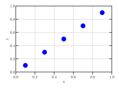
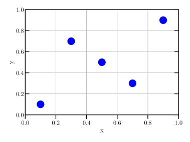
Figure 1: Two possible Latin hypercubes in a two dimensional parameter space normalized to the unit square. The left example covers only a one-dimensional subspace and hence would be rejected. The right example has support throughout the whole two dimensional parameter space and would produce a better emulator.

The Gaussian process kernel described in section 2.3 has an uncertainty roughly proportional to the distance between a parameter vector and the nearest simulation. In order to minimize the maximum error, we would like to spread our simulations evenly throughout parameter space. We would also like to avoid simulations clustered in low-dimensional sub-spaces, which would be unable to reproduce parameter variations elsewhere.

To ensure these properties, we choose the sampling points for our simulations using a Latin hypercube, as have been used extensively in cosmological emulators [29]. This structure divides a (normalized) parameter space into a regular grid, with as many rows in each dimension as sampling points. Thus for an emulator with $n$ dimensions containing $k$ simulations we would first create a $k^{n}$ grid. The samples are placed in turn such that no sample overlaps in any dimension. Each sample added thus blocks off one row in all $n$ dimensions. This is equivalent to choosing a random permutation of the integers $0-k$ [24] and ensures that once the samples are projected to a single dimension, they evenly sample the unit interval. Note that there is no restriction on the number of simulations that can be placed within a given parameter space.

There are a large number of possible Latin hypercubes and not all of them ensure our desired properties. Figure 1 shows two, for $n=2$ and $k=5$. We would like to avoid Latin hypercubes which fill only a one-dimensional subspace of parameter space, as in the left example. The most common technique for ensuring space-filling properties is to use orthogonal Latin hypercubes, which enforce uniform sampling not just in each parameter, but in each $2$ or $3$-dimensional subspace. However, these designs are inflexible and not suited to adding extra simulation points.

Instead, we use a Monte Carlo approach. We generate $10,000$ hypercubes at random and use the one which maximizes our space-filling metric, discarding the rest. Our space-filling metric is the sum of the Euclidean distances between each point in the hypercube and its closest neighbour. This approach is simple, computationally efficient, and allows for the addition of extra simulation points to the design in a later refinement step, as in our companion paper ref. [38]. The right panel of Figure 1 shows a simple Latin hypercube generated using this procedure, demonstrating that these samples achieve good coverage of parameter space.

2.4.2 Quadratic emulator: single parameter grid

Figure 2: Locations of the sampling points for a quadratic emulator in a (normalized) two-dimensional parameter space for a “best-fit” simulation at $(0.5,0.5)$. Our emulator uses $4n+1$ simulations.

In order to compare our new emulator techniques to prior work, we also generate a ‘quadratic’ emulator similar to ref. [7]. First a “best-fit” set of parameters is simulated, chosen to lie at the midpoint of each dimension in the $n$-dimensional parameter space prior volume. For our quadratic emulator, this parameter combination is: $\tau_{0}=1$, $d\tau_{0}=0$, $n_{s}=0.8975$, $A_{\mathrm{P}}=1.9\times 10^{-9}$, $H_{S}=-0.3$, $H_{A}=0.9$, $h=0.7$. Each simulation varies only one parameter from this midpoint. Each bin of the resulting flux power spectra is fit with a quadratic polynomial, and interpolation evaluates each quadratic polynomial at the new parameters. We run four simulations for each parameter, for a total of $4n+1$ simulations. Although this procedure may seem simplistic, and does not capture variations involving multiple parameters, it can work reasonably well [7], because the flux power spectrum varies almost linearly in the Lyman-$\alpha$ forest parameters (see appendix A).

2.5 Likelihood

In this section we describe our likelihood function. The previous sections have described how we can generate a flux power spectrum for arbitrary input cosmological parameters. While we will see that our procedure can do this with a reasonable degree of accuracy, an important advantage of the Gaussian process is that it also provides an estimate of the error in the interpolation. This estimate can be used to propagate interpolation error into posterior probabilities. In principle (as long as the actual interpolation error is approximately Gaussian), this should cause moderate interpolation error to increase uncertainty, without leading to a bias in the derived cosmological parameters. Our likelihood is sampled using the emcee package [57].

We use a simple quadratic (log) likelihood function, given by

$$\log\mathcal{L}(p_{k}) =-\frac{1}{2}C^{-1}_{ij}(p_{k})dP_{i}(p_{k})dP_{j}(p_{k})-\frac{1}{2}\log\mathrm{det}\,C_{ij}(p_{k})$$ (2.11)

$$dP_{i}(p_{k}) =P^{\mathrm{sim}}_{F}(k_{i},p_{k})-P_{F}^{\mathrm{data}}(k_{i})\,,$$ (2.12)

where $C_{ij}(p_{k})$ is the total covariance matrix and $P^{\mathrm{sim}}_{F}(k_{i},p_{k})$ the simulated flux power spectrum for a set of parameters $p_{k}$. $P^{\mathrm{data}}(k_{j})$ is the flux power spectrum of the mock data. We impose a hard prior on all parameters that they must be within the parameter bounds of the simulated emulator given in Table 1.

The covariance matrix $C_{ij}$ is the sum of the total BOSS DR9 covariance from ref. [14] and the emulator error generated by the Gaussian process

$$C_{ij}(p_{k})=C_{ij}^{\mathrm{BOSS}}+C_{ij}^{\mathrm{GP}}(p_{k})\,.$$ (2.13)

While $C_{ij}^{\mathrm{BOSS}}$ does not depend on cosmology, $C_{ij}^{\mathrm{GP}}(p_{k})$ does, depending primarily on the distance between $p_{k}$ and the nearest simulation point, and has an amplitude which is related to a hyper-parameter of the Gaussian process ($\sigma_{0}$). Because $C_{ij}(p_{k})$ thus depends on $p_{k}$, every likelihood evaluation requires a matrix inversion. Furthermore, in principle $\log\mathrm{det}\,C_{ij}$ is not constant and cannot be absorbed into the likelihood normalization, although in practice we find that it does not vary significantly. The need to invert matrices slows down likelihood computation only moderately: evaluating our Gaussian Process likelihood is a factor of two slower than the quadratic likelihood.

For a Gaussian process with single-valued output, the covariance matrix would be diagonal and given by $\sigma^{2}(p_{i})$, the Gaussian process expected error at parameters $p_{i}$. However, we found a substantial correlation in the actual error between each $k$-bin. This can be understood because, as detailed in section 2.3, our Gaussian process uses the same hyper-parameters to estimate all scales in a single redshift bin. There are also substantial correlations between different $k$-bins in the 1D Lyman-$\alpha$ flux power spectrum, because it probes non-linear scales. In order to ensure that we do not bias the likelihood, we conservatively assume that all $k$-bins at the same redshift are maximally correlated, minimizing the information content. However, because each redshift bin has separate hyper-parameters, we approximate the correlations in emulator error as zero if two data points are in different redshift bins. The covariance matrix for the emulator is thus

$$C_{ij}=\sigma(z_{i},p_{i})\delta_{z_{i}z_{j}}\,,$$ (2.14)

where $\sigma(z_{i},p_{i})$ is the error reported by the Gaussian process at the parameter vector $p_{i}$ at redshift bin $z_{i}$, and $\delta_{z_{i}z_{j}}$ is unity if $i$ and $j$ are at the same redshift and zero otherwise.

As detailed in section 2.1, we generate an interpolated flux power spectrum $P^{\mathrm{sim}}_{F}(k_{i},p_{k})$ at values of $k^{\mathrm{box}}_{i}$ which are multiples of the simulation box (“Fourier” units). Thus, we rebin the flux power spectrum so that it is evaluated at values of $k_{i}$ which are the same as those in BOSS DR9. Since our simulation boxes are relatively small, the largest scales measured by BOSS are on scales larger than the simulation box and are omitted from the likelihood.

As our simulations are not resolved, and to preserve the option of blinding any later analysis with larger simulations, we do not use the actual BOSS flux power spectrum measurement for $P^{\mathrm{data}}(k_{j})$. Instead we have performed a series of $6$ test simulations. The parameters of these test simulations were generated at random using a Latin hypercube (as in the main emulator, section 2.4.1) with slightly restricted cosmological parameter limits: $n_{s}=0.9-0.99$ and $A_{\mathrm{P}}=1.4\times 10^{-9}-2.6\times 10^{-9}$. This ensures that our tests cover our prior volume but that some of our likelihood posteriors are separated from the emulator bounds.

3 Results

In this section we describe the performance of our emulator methods. In section 3.1 we describe the ability of our Gaussian process emulator to accurately interpolate the flux power spectrum. We compare to a quadratic polynomial emulator in section 3.2. Then in section 3.3 we show posterior probabilities generated from likelihood functions using both the Gaussian process and quadratic emulators. We demonstrate that the true parameters lie within the $68\%$ confidence intervals of the likelihood when using our Gaussian process, with smaller parameter errors than the quadratic emulator. To aid the reader in visualising our results, figure 3 shows the flux power spectra from our test simulations, whose parameters provide the ground truth to which we compare our emulation and Markov Chain results.

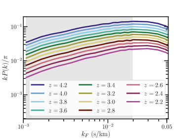
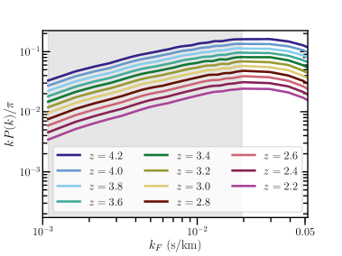
Figure 3: Flux power spectra extracted from two of our test simulations. Each line represents a different redshift bin. The grey shaded region shows the scales measured by BOSS. (Left) Test simulation parameters are $\tau_{0}=0.9$, $d\tau_{0}=0$, $n_{s}=0.907$, $A_{s}=1.7\times 10^{-9}$, $H_{A}=0.933$, $H_{S}=-0.633$, $h=0.742$. (Right) Test simulation parameters are $\tau_{0}=0.9$, $d\tau_{0}=0$, $n_{s}=0.982$, $A_{s}=2.5\times 10^{-9}$, $H_{A}=0.667$, $H_{S}=-0.1$, $h=0.658$.

3.1 Gaussian process emulator accuracy

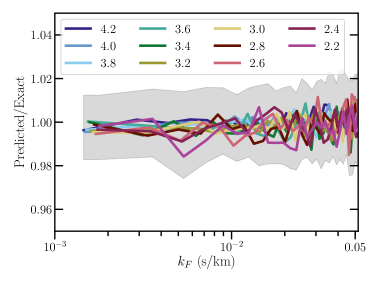
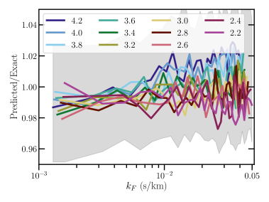
Figure 4: Accuracy of the Gaussian process emulator. We show the ratio between an emulated flux power spectrum and the true flux power spectrum from a simulation with the same set of cosmological parameters. Each line represents a different redshift bin. The grey band shows the expected error from the emulator. For clarity we show the maximum region covered by the $1-\sigma$ emulator error prediction. This is larger than the true difference, both because it combines multiple redshift bins and because the emulator slightly over-estimates the true error at these parameters. (Left) Test simulation parameters are $\tau_{0}=0.9$, $d\tau_{0}=0$, $n_{s}=0.907$, $A_{s}=1.7\times 10^{-9}$, $H_{A}=0.933$, $H_{S}=-0.633$, $h=0.742$. (Right) Test simulation parameters are $\tau_{0}=0.9$, $d\tau_{0}=0$, $n_{s}=0.982$, $A_{s}=2.5\times 10^{-9}$, $H_{A}=0.667$, $H_{S}=-0.1$, $h=0.658$.

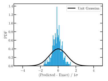
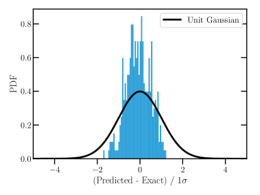
Figure 5: Distribution of the errors of the Gaussian process for the same test simulations in figure 4. We show a histogram of the actual difference in each $k$ and $z$ bin between the flux power spectrum estimated from the emulator and the true flux power spectrum from a simulation, normalized by the $1-\sigma$ error expected from the emulator. Shown for comparison is a unit Gaussian. Thus an ideal error estimation would result in a match between the black line and the blue histogram. Each figure shows a different simulation with $11$ independent redshift bins and $31$ correlated $k$-bins. For these two simulations the Gaussian process is slightly over-estimating the true errors. In other test simulations the Gaussian process expected error is more accurate. (Left) Test simulation parameters are $\tau_{0}=0.9$, $d\tau_{0}=0$, $n_{s}=0.907$, $A_{s}=1.7\times 10^{-9}$, $H_{A}=0.933$, $H_{S}=-0.633$, $h=0.742$. (Right) Test simulation parameters are $\tau_{0}=0.9$, $d\tau_{0}=0$, $n_{s}=0.982$, $A_{s}=2.5\times 10^{-9}$, $H_{A}=0.667$, $H_{S}=-0.1$, $h=0.658$.

Figure 4 shows the accuracy of a Gaussian process emulator using the cosmological parameters for two test simulations. The parameter file for the simulations used, as well as the flux power spectra, are available from https://github.com/sbird/lya_emulator_training/. We tested the accuracy of our Gaussian process emulator with six test simulations not included in the emulator, as described in section 2.5. From these six we show in the left panel one simulation where the accuracy of the emulator was typical, and in the right panel the test simulation where the accuracy was poorest. We show the differences in each redshift bin between the flux power spectrum generated by the emulator and that from a test simulation. The typical difference between the Gaussian process prediction and the simulated flux power spectrum is of the order of $1\%$, with a worst-case performance of $2\%$ (although the estimated emulator error, shown by the grey band in figure 4, is larger). We further tested the Gaussian process emulator using the input simulations, which were reproduced to machine precision, and using the $21$ simulations run for the quadratic emulator. The latter had similar performance to the other $6$ test simulations, and showed that the emulator is generally accurate to $\sim 1\%$, with only $6/27$ simulations showing $>2\%$ inaccuracy. For comparison, the current statistical error on the BOSS DR9 1D flux power spectrum is minimal at around $\sim 3\%$ at $z=2.4$, rising to $6\%$ at $z=3.6$ and $\sim 10\%$ at $z\geq 4$. Figure 4 thus demonstrates that our emulator is capable of achieving the percent-level accuracy required for both current and next-generation Lyman-$\alpha$ surveys.

Notice that the residual errors are often correlated between neighbouring $k$-bins, but that the largest and smallest scales are uncorrelated. Furthermore, there appears to be little correlation between neighbouring redshift bins, justifying the assumptions of our likelihood function. For this emulator, error is usually worst on small scales. This has a simple explanation: small scales are more non-linear and thus inherently harder to model. Furthermore, the IGM thermal history affects the shape of the flux power spectrum only on small scales. Thus the emulator has to fit more complex variations over more parameters at these scales. Recovery of the power spectrum appears to be worse at high redshift in the right-hand plot of Figure 4, but this is a feature specific to this test case: there is no general trend of interpolation error with redshift.

Figure 5 shows histograms of the actual errors normalized by the expected error from the Gaussian process. Also shown is a unit Gaussian. If the emulator’s error estimation was correct, the histograms should be close to the unit Gaussian. We can see that for these two examples the Gaussian process is moderately over-estimating the true error. This is mostly due to a statistical fluctuation in these two test simulations. Other test simulations showed an error distribution closer to the unit Gaussian, and a histogram combining errors from all our test simulations was much closer. None of our test simulations showed the emulator under-estimating the error, but $3/27$ tests showed $>1-\sigma$ offset between the true error distribution and the unit Gaussian, indicative of a biased estimate of the flux power spectrum. Overall, we found that it was more difficult for the Gaussian process to accurately estimate errors than to produce a good estimate of the flux power spectrum.

3.1.1 Emulator accuracy

The overall accuracy of the emulator is controlled by the density of simulations. From the radial basis function kernel, eq. 2.8, the emulator error scales like

$$E=E_{0}\frac{\Delta x}{\sqrt{2}l}\,,$$ (3.1)

where $\Delta x$ is the distance to the nearest simulation point, in units where all parameters are mapped onto the unit cube. For our emulator the RBF length scale is $l=2.5-3$, depending on the redshift. For evenly spaced simulations, the maximum distance from any point to the nearest simulation is

$$\Delta x\sim\sqrt{\frac{P}{N_{\mathrm{sim}}^{2}}}\,,$$ (3.2)

where $N_{\mathrm{sim}}$ is the number of simulations and $P$ is the number of parameters. For us $N_{\mathrm{sim}}=21$ and $P=7$, so $\Delta x\approx 0.13$. We achieve an average error of $1.5\%$, so if $l=3$, $E_{0}\approx 0.5$. Inverting Eq. 3.1 shows that the emulator error scales linearly with the number of simulations and that a median error of $\sim 4\%$ would require only $8$ simulations. A median emulator error larger than the statistical error in the data can present difficulties for parameter estimation, as the covariance matrix becomes highly parameter dependent, in extreme cases leading to a multi-modal likelihood.

This calculation, however, neglects an important source of uncertainty in the emulator; the need to estimate the kernel hyper-parameters. For sparse data it becomes extremely difficult to determine the optimal hyper-parameter and thus the emulator is inaccurate. Worse, because the emulator error is itself a hyper-parameter this source of error is not included in the emulator’s error estimate and thus the posterior confidence intervals become biased. We have been unable to find firm guidance in the statistics literature as to what simulation point density is necessary for a good hyper-parameter estimation. A reasonable ansatz seems that the kernel length scale should be at least the average distance between simulations: $\Delta x=\sqrt{P}/N=Kl$. Note that $l$ corresponds to a physical scale of variation in the flux power spectrum and so the number of simulations needed will scale with the prior parameter volume. The value of $K$ is uncertain, and is likely to depend on the exact form of the kernel. As the hyper-parameters of our Gaussian process emulator are well-determined, we know that $K\lesssim 20$. An earlier iteration of our test emulator with a prior volume $5$ times larger did not have well-determined hyper-parameters, suggesting that for our kernel $K\gtrsim 5$.

3.2 Comparison to a quadratic emulator

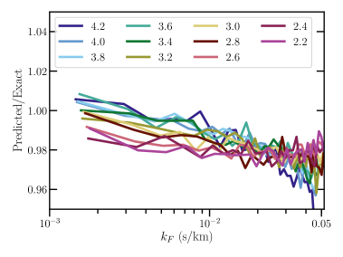
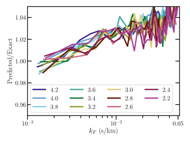
Figure 6: Accuracy of the emulator using quadratic polynomial interpolation. We show the ratio between an emulated flux power spectrum and the true flux power spectrum from a simulation with the same set of cosmological parameters. Each line represents a different redshift bin. Test simulation parameters are identical to those used in figure 4. (Left) Test simulation parameters are $\tau_{0}=0.9$, $d\tau_{0}=0$, $n_{s}=0.907$, $A_{s}=1.7\times 10^{-9}$, $H_{A}=0.933$, $H_{S}=-0.633$, $h=0.742$. (Right) Test simulation parameters are $\tau_{0}=0.9$, $d\tau_{0}=0$, $n_{s}=0.982$, $A_{s}=2.5\times 10^{-9}$, $H_{A}=0.667$, $H_{S}=-0.1$, $h=0.658$.

Figure 6 shows the accuracy of a quadratic polynomial emulator, using the same test simulations, prior parameter ranges and number of simulations as the Gaussian process shown in figure 4. A comparison between figures 4 and 6 thus shows directly the relative performance of each emulator. We find that the overall accuracy of our quadratic emulator at these test points is around $4\%$. Two of our six test simulations achieved $2\%$ accuracy. This performance is clearly worse than the Gaussian process emulator. Furthermore, figure 6 shows that the error is highly correlated between redshift bins, which may present a difficulty for parameter estimation. Note that we have generated test spectra at $\tau_{0}=0.9$, whereas the quadratic emulator is centered on $\tau_{0}=1$. The value of $\tau_{0}$ at which the quadratic emulator is evaluated strongly changes the overall accuracy. In fact, at $\tau_{0}=1$, the quadratic emulator performs almost as well as the Gaussian process emulator. This is not surprising, as the mean flux, $\tau_{0}$, is the single parameter which most affects the flux power spectrum. However, the accuracy of the quadratic emulator degrades quickly as the mean flux changes. As the quadratic emulator only varies one parameter at a time, all simulations except the central one have their flux power spectra generated at $\tau_{0}=1$, and any correlation between power spectrum shape variation from the mean flux and from cosmology is not captured. This sensitivity to the mean flux is not seen in the Gaussian process emulator, which generates a series of flux power spectra with different mean fluxes for every simulation. Figure 8 shows that posterior error on the mean flux is around $\Delta\tau_{0}=0.1$ so the quadratic emulator is always inaccurate in some part of the $68\%$ confidence intervals.

We also note that the overall accuracy of the quadratic emulator is sensitive to the prior parameter range. Although the quadratic emulator shown here has an accuracy of only $4\%$, quadratic emulators used in prior work [e.g  26, 7, 14] have achieved better performance by using a restricted prior parameter range, or by carefully choosing the simulated parameters to lie close to the best fit value of the model. However, this is not always possible, as the emulator must encompass the full data posterior, and the best fit of the model may not be known in advance.

We also tested running a Gaussian process emulator using as input the single-parameter grid of simulations performed for the quadratic emulator. This reveals whether the improvement of the Gaussian process over the quadratic emulator was due to the sampling strategy or the more flexible interpolation algorithm. Since the kernel chosen for the Gaussian process includes a dot kernel, which is equivalent to linear interpolation, we expect the Gaussian process to do at least as well as quadratic emulation. Of our $6$ test simulations, $4$ test simulations achieved $\sim 1\%$ accuracy, similar to the full Gaussian process emulator. However, the other $2$ test simulations showed $\sim 4\%$ accuracy, similar to the quadratic emulator, although the simulations with the poorest estimation were not the same.

With a single parameter grid the Gaussian process over-estimated the emulator error by a factor of $4-10$. This has a simple explanation. The quadratic emulator relies on varying each parameter in the emulator separately and combining them, which is reasonably accurate in practice. However, without simulations which vary multiple parameters at once the Gaussian process does not know this and is thus unable to properly constrain the emulator error. It thus seems that the majority of the improved emulator performance with our Gaussian process comes from the improved sampling strategy. We infer that the chief limitation of the quadratic polynomial interpolation is that it forces a sampling strategy with a relatively limited coverage of parameter space, especially away from the central mean flux value.

3.3 Posterior parameter constraints

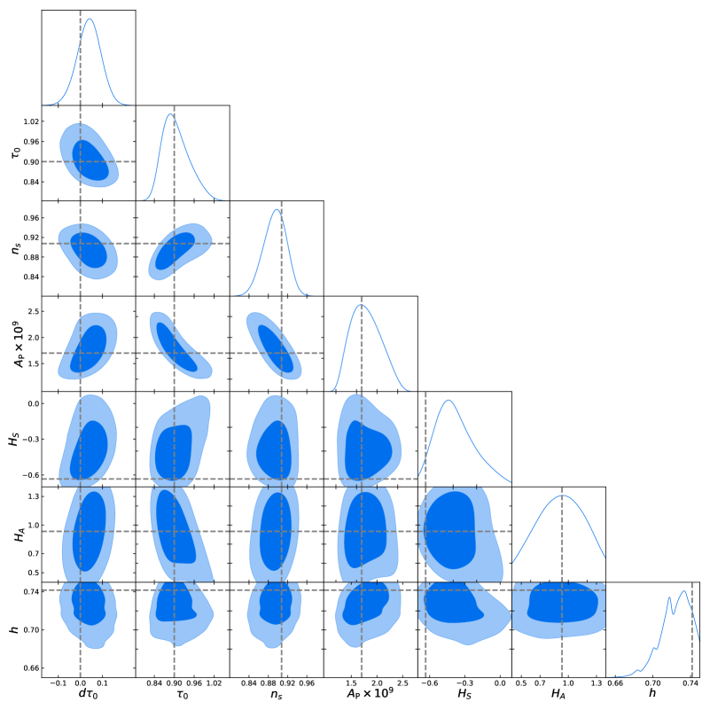
Figure 7: Marginalized likelihood posteriors in $1D$ and $2D$ for the parameters of our test simulation with $\tau_{0}=0.9$, $d\tau_{0}=0$, $n_{s}=0.907$, $A_{s}=1.7\times 10^{-9}$, $H_{A}=0.933$, $H_{S}=-0.633$, $h=0.742$ using a $21$ sample Gaussian process emulator. Contours show $68\%$ and $95\%$ confidence intervals. The true parameter values are shown by dashed lines.

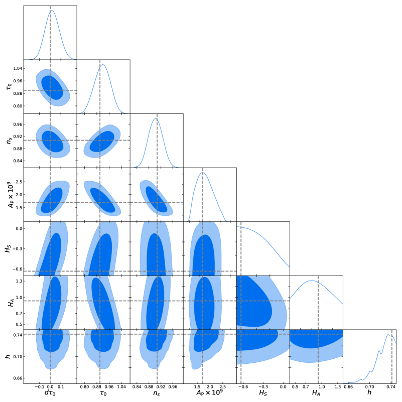
Figure 8: Marginalized likelihood posteriors in $1D$ and $2D$ for the parameters of our test simulation with $\tau_{0}=0.9$, $d\tau_{0}=0$, $n_{s}=0.907$, $A_{s}=1.7\times 10^{-9}$, $H_{A}=0.933$, $H_{S}=-0.633$, $h=0.742$ using a $21$ sample quadratic polynomial emulator. Contours show $68\%$ and $95\%$ confidence intervals. The true parameter values are shown by dashed lines.

Parameter	Gaussian process	Quadratic	Quad/GP (%)
$d\tau_{0}$	$-0.014$ - $0.092$	$-0.046$ - $0.086$	$25$
$\tau_{0}$	$0.866$ - $0.947$	$0.864$ - $0.967$	$26$
$n_{s}$	$0.87$ - $0.92$	$0.88$ - $0.97$	$-3$
$A_{\mathrm{P}}\times 10^{9}$	$1.484$ - $2.094$	$1.464$ - $2.140$	$11$
$H_{S}$	$-0.54$ - $-0.20$	$-0.61$ - $-0.15$	$34$
$H_{A}$	$0.65$ - $1.18$	$0.58$ - $1.19$	$16$
$h$	$0.71$ - $0.74$	$0.71$ - $0.74$	$4$

Table 2: Table of $68\%$ posterior parameter confidence intervals from the Gaussian process and quadratic emulators. The final column shows the percentage change in the confidence interval widths. Positive numbers indicate wider intervals in the quadratic emulator. The true parameter values of the input simulation are $\tau_{0}=0.9$, $d\tau_{0}=0$, $n_{s}=0.907$, $A_{s}=1.7\times 10^{-9}$, $H_{A}=0.933$, $H_{S}=-0.633$, $h=0.742$

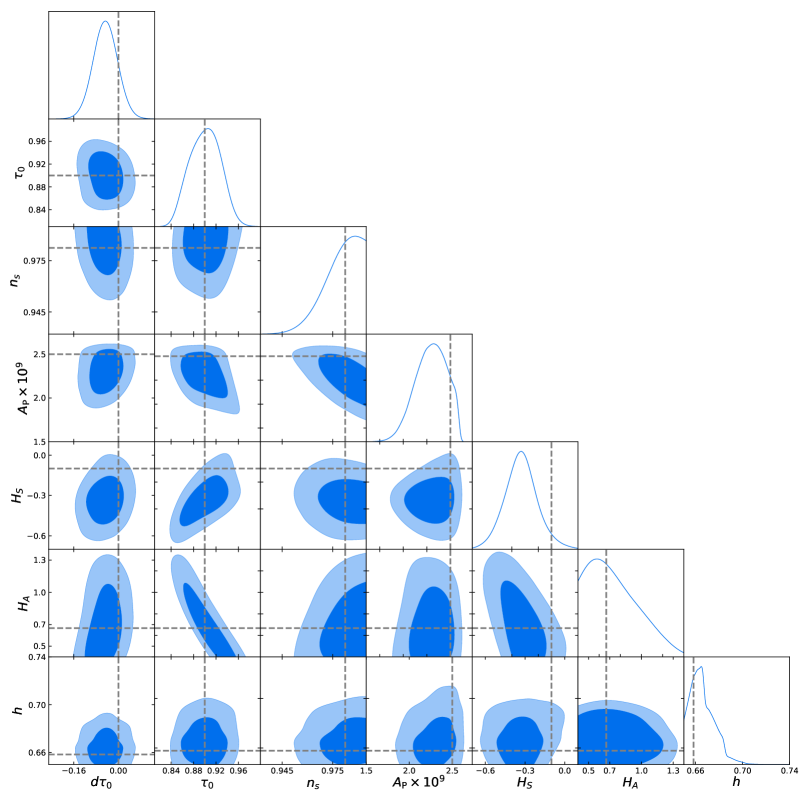
Figure 9: Marginalised likelihood posteriors in $1D$ and $2D$ for the parameters of our test simulation with $\tau_{0}=0.9$, $d\tau_{0}=0$, $n_{s}=0.982$, $A_{s}=2.5\times 10^{-9}$, $H_{A}=0.667$, $H_{S}=-0.1$, $h=0.658$ using a $21$ sample Gaussian process emulator. Contours show $68\%$ and $95\%$ confidence intervals. The true parameter values are shown by dashed lines.

Figure 7 shows the $1D$ and $2D$ posterior parameter constraints from the Gaussian process emulator on a test simulation. The emulator error at the true data points of the simulation is shown in figure 4, and is typical for test simulations using this emulator. With emulator errors at this level ($1-2\%$ of the flux power spectrum), the posterior confidence intervals provide an unbiased measurement of the true parameter values. Some of the thermal parameters are poorly constrained by the BOSS data. In particular the $95\%$ marginalized confidence intervals on $H_{A}$ and $H_{S}$ overlap with the emulator prior volume. Ref. [15] find $\Delta\gamma=0.2$ and $\Delta T_{0}=3500$ K at $68\%$ confidence. When translated into constraints on $\gamma$ and $T_{0}$, our prior volume has $\Delta\gamma=0.4$ and $\Delta T_{0}=9000$ K (see section 2.2), so our results are consistent. These relatively poor constraints are expected with the BOSS DR9 covariance, which does not measure the small scales that are most sensitive to the thermal history. We considered enlarging our prior volume, but there are strong physical reasons to expect $\gamma$ and $T_{0}$ to be within this range. Alternatively, we considered placing a prior on $T_{0}$ from high resolution flux power spectrum measurements, but again decided against it because we wished to demonstrate that our emulator produces unbiased results throughout the prior volume. Our constraints on $\tau_{0}$ are much tighter than our prior volume.

The Gaussian process emulator shows parameter degeneracies between $A_{\mathrm{P}}$, $n_{s}$ and $\tau_{0}$, including a curved degeneracy between $A_{\mathrm{P}}$ and $\tau_{0}$. This is to be expected, since $A_{\mathrm{P}}$ and $\tau_{0}$ both set the overall amplitude of the flux power spectrum. The degeneracy between $n_{s}$ and $A_{\mathrm{P}}$ suggests that, once the thermal parameters are marginalized out, the scale at which the Lyman-$\alpha$ forest is most sensitive to cosmology is larger than the pivot scale we chose, $k_{\mathrm{P}}=0.78$ Mpc^-1. This motivates a smaller $k_{\mathrm{P}}$ in future work.

Our constraints on $h$ appear unusually tight: $\Delta h=0.04$ at $68\%$ confidence ignoring prior volume effects. They also exhibit unusual non-smooth features in the likelihood. Recall from section 2.2 that we hold $\Omega_{M}h^{2}$ constant and so a variation in $h$ is also a variation in $\Omega_{M}$. Most of the constraining power is thus coming from the effect of $\Omega_{M}$ on the growth rate of the cosmological perturbations at this redshift. The non-smooth likelihood features arise from our choice to ignore data on scales larger than our simulation box size. Since the mapping between the size of the simulation box (in comoving Mpc/h) to the measured bins of the flux power spectrum (in physical km/s) depends on $\Omega_{M}$ (eq. 2.1), decreasing $h$ causes an extra flux power spectrum bin to be included in the likelihood, suddenly reducing the error bars. This feature would not occur in an emulator with a larger box.

Figure 8 shows the posterior parameter constraints using the quadratic emulator. The true parameter values again all lie within the $68\%$ confidence intervals, but the constraints on key cosmological parameters are substantially weaker. The $68\%$ marginalized confidence intervals are given in Table 2. Increases in the confidence interval widths are largest in the thermal parameters, $H_{S}$ and $H_{A}$, which have the most non-linear effect on the flux power spectrum (see Appendix A). Constraints on the primordial power spectrum amplitude, $A_{\mathrm{P}}$ are also weaker, due to the degeneracy between $A_{\mathrm{P}}$ and $\tau_{0}$.

The quadratic polynomial emulator has larger emulator error, but our likelihood function does not include it in the covariance matrix. We might thus naively expect a biased parameter value rather than larger uncertainty. However, the true change in the flux power spectrum at parameter values away from the central “best-fit” simulation for several parameters, in particular $\tau_{0}$, is larger than estimated by the quadratic polynomial. This leads to the emulator under-estimating the constraining power of the data, leading to larger uncertainties, and these larger uncertainties are sufficient to dominate over biased parameters from an inaccurate likelihood. Note that the magnitude of the difference in posterior errors depends on the specific prior volume and dataset used.

Figure 9 shows the posterior likelihood constraints for the second test simulation shown in figure 4, for a Gaussian process emulator. This simulation serves as a useful worst-case scenario for our Gaussian process emulator as this test simulation had the largest error between the emulated and true flux power spectra. In this case the emulator error is $3-4\%$, comparable to the diagonal elements of the BOSS covariance matrix at low redshift. However, with the exception of $H_{S}$, the true parameter values are within the $68\%$ confidence intervals, demonstrating that the emulator produces unbiased parameters. We examined the posterior contours for the other $4$ test simulations and in all other cases the true parameter values lay within the $68\%$ confidence intervals. Furthermore, in all cases the quadratic polynomial emulator produced weaker constraints than the Gaussian process emulator, with the increase in the size of the contour widths similar to those already discussed.

We checked the effect of artificially setting emulator error to zero in the likelihood function using our test simulations. For the worst-case test simulation shown in figure 9 posterior confidence interval widths shifted by $\sim 10\%$, with the constraints on $n_{s}$ tightening and those on $H_{S}$ weakening. The posterior contours continued to enclose the true parameter values within the $68\%$ confidence intervals. We caution that this continued unbiased estimation of the posterior may simply be because the emulator is moderately over-estimating the true error for this test point (see figure 5). For our other test simulations there was minimal effect on the posterior confidence intervals, probably because the emulator error in these cases was $<50\%$ of the statistical error from BOSS DR9.

4 Conclusions

We have constructed and validated techniques for emulation of the Lyman-$\alpha$ forest 1D flux power spectrum. We have not yet performed simulations of sufficient size to produce a resolved flux power spectrum, instead using this paper to validate our emulator building routines with a series of small, $40$ Mpc/h, simulations with $2\times 256^{3}$ particles. We sample $5$ parameters with $21$ simulations in a Latin hypercube scheme. There are $2$ parameters describing the thermal history of the IGM and $3$ describing cosmology. We add a further $2$ parameters for the mean flux in post-processing. Our emulator allows the generation of 1D Lyman-$\alpha$ forest flux power spectra at arbitrary parameter values within the emulator volume, unlike existing interpolation methods which only perform well near a fiducial simulation. A Gaussian process is used for interpolation, with a kernel including both linear and radial basis function terms.

We tested our emulator with a series of $6$ simulations spread throughout parameter space. The typical interpolation error was $1\%$, with a worst-case performance of $4\%$, comparable to the BOSS DR9 1D Lyman-$\alpha$ forest flux power spectrum statistical error of $3-10\%$ [14]. The Gaussian process estimates the interpolation error as well as the function value at the interpolation point. We demonstrated that in our test simulations the estimate of this error is reasonably reliable. It was accurate in $4$ of our $6$ tests and moderately larger than the true emulator error in the other $2$.

We constructed a likelihood function for our emulator using our test simulations and the BOSS DR9 data covariance matrix as mock data. The likelihood function propagated the estimated emulator error from the Gaussian process, and thus accounted for residual interpolation error. We showed that MCMC chains run using our likelihood function were able to recover the true parameters of the test simulation, within $68\%$ confidence intervals. Interestingly, an earlier test emulator with a prior volume five times larger did not produce unbiased posterior results, and showed distinctly non-Gaussian error residuals. This suggests that for the Gaussian process to produce an unbiased posterior estimate requires a critical density of simulation points. We suggest that the this density must be sufficient for accurate optimization of kernel hyper-parameters. We considered the effect of artificially setting the expected emulator error to zero in our likelihood, and discovered that it was small in most cases, as for our emulator the estimated error is much smaller than the data covariance.

We compared our Gaussian process emulator to a quadratic polynomial emulator resembling those used by earlier Lyman-$\alpha$ forest analyses, showing that it produced substantially smaller emulator error (by a factor of $2$) with the same number of simulations and prior volume. To evaluate the impact on posterior parameter constraints, we ran MCMC chains using our quadratic emulator and showed that posterior confidence intervals using a typical test simulation were on average $16\%$ wider. We (reassuringly) showed that the quadratic emulator did not produce biased parameter constraints. The emulator error for quadratic interpolation was around $4\%$, which suggests that although it is sufficient for data with statistical uncertainties of $\sim 10\%$ such as in ref. [58], it will be inadequate for future datasets with smaller statistical error. The techniques and code we present in this work will thus be essential for making best use of future Lyman-$\alpha$ forest surveys.

Similar emulators would also be useful for Lyman-$\alpha$ forest datasets derived from high resolution spectra. These datasets probe smaller scales, up to $k=0.2$ s/km [11] and are generally more sensitive to the details of reionization and the thermal history of the IGM. The simulations presented here are not of sufficient resolution to probe these scales with fidelity, so we have not attempted to build an emulator for them here. However, it should be possible to build a similar emulator to ours for these scales using higher resolution simulations and a model for reionization.

Although our focus in this paper has been the Lyman-$\alpha$ forest, the techniques of cosmological emulation are generally applicable to any problem which requires expensive forward simulation, in particular those sensitive to non-linear gravitational evolution. Such problems include galaxy clustering, weak lensing, 21cm and the halo mass function, most of which have had emulators constructed for them. The most generally applicable points in this paper are our use of a flexible Latin hypercube design which maximizes the coverage of simulation points, our understanding of the importance of good hyper-parameter estimation and that this can be improved using multi-output Gaussian processes.

In a companion paper, ref. [38], we show how the Lyman-$\alpha$ emulator can be improved by Bayesian emulator optimization, which iteratively adds points to the simulation sample set, and produces further improvements in the width of posterior confidence intervals. In these two papers we have demonstrated that the techniques presented here are capable of achieving the percent-level accuracy necessary for an optimal analysis of future Lyman-$\alpha$ forest surveys, such as DESI. In future work we will apply our techniques to building a full cosmological emulator for the Lyman-$\alpha$ forest. We will also incorporate more sophisticated models of hydrogen and helium reionization, which will allow us to improve the fidelity of our modelling as well as the interpolation error.

Appendix A Single-parameter variations

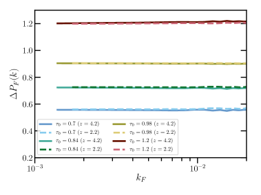
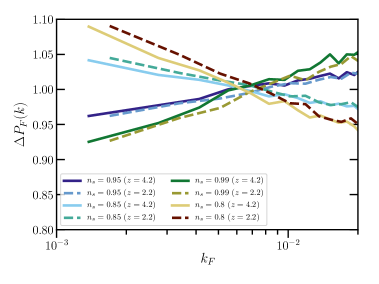
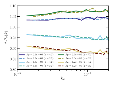
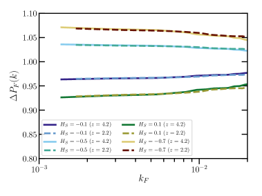
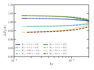
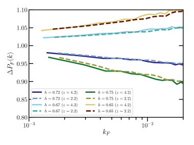
Figure 10: The effects of changing each emulator parameter on the 1D flux power spectrum. Shown is the ratio between the flux power spectrum at each parameter value used for the quadratic emulator to the “best-fit” simulation at $\tau_{0}=1$, $d\tau_{0}=0$, $n_{s}=0.8975$, $A_{\mathrm{P}}=1.9\times 10^{-9}$, $H_{S}=-0.3$, $H_{A}=0.9$, $h=0.7$. The parameters are: (top-left) the mean flux $\tau_{0}$, (top-right) the spectral index $n_{s}$, (middle-left) the primordial power spectrum amplitude $A_{\mathrm{P}}$, (middle-right) the heat slope $H_{S}$, which controls the temperature-density relation parameter $\gamma$, (bottom-left) the heat amplitude $H_{A}$, which controls the temperature at mean density $T_{0}$ and (bottom-right) the hubble parameter, $h$, which is inversely proportional to the matter density $\Omega_{M}$ in our scheme. We show the minimum and maximum redshifts in the emulator: $z=2.2$ (dashed) and $z=4.2$ (solid).

Figure 10 shows the effect on the 1D flux power spectrum of changing a single parameter in our emulator, using the simulations from the quadratic polynomial emulator. While this has been discussed in the literature before [e.g. ref  6], we have interpolated a non-standard set of parameters, and so in the interests of clarity we show how our new parameters affect the flux power spectrum. We show the effect at $z=2.2$ and $z=4.2$ to demonstrate that the change in each parameter with redshift is relatively small. The redshift-dependent conversion between km/s and comoving Mpc/h is visible as specific features, including the box size, move with redshift. The degeneracy between $\tau_{0}$ and $A_{\mathrm{P}}$ is also visible, although this would be partially broken by the largest scale bin if our box size was increased. We have rescaled each spectrum to have the same mean flux. Increasing the IGM temperature using $H_{A}$ increases the flux power spectrum only on the relatively large scales shown (and only because we must match the mean flux). On smaller scales it erases power, as expected.

References

- [1] Planck Collaboration, P. A. R. Ade, N. Aghanim, M. Arnaud, M. Ashdown, J. Aumont et al., Planck 2015 results. XIII. Cosmological parameters, AAP 594 (2016) A13 [1502.01589].
- [2] R. A. C. Croft, D. H. Weinberg, N. Katz and L. Hernquist, Recovery of the Power Spectrum of Mass Fluctuations from Observations of the Lyman-alpha Forest, ApJ 495 (1998) 44 [astro-ph/9708018].
- [3] SDSS collaboration, P. McDonald et al., The Lyman-alpha Forest Power Spectrum from the Sloan Digital Sky Survey, ApJ Supplement 163 (2006) 80 [astro-ph/0405013].
- [4] M. Viel, G. D. Becker, J. S. Bolton and M. G. Haehnelt, Warm dark matter as a solution to the small scale crisis: New constraints from high redshift Lyman- forest data, PRD 88 (2013) 043502 [1306.2314].
- [5] U. Seljak, A. Slosar and P. McDonald, Cosmological parameters from combining the Lyman- forest with CMB, galaxy clustering and SN constraints, JCAP 10 (2006) 014 [astro-ph/0604335].
- [6] M. Viel, M. G. Haehnelt and A. Lewis, The Lyman forest and WMAP year three, MNRAS 370 (2006) L51 [astro-ph/0604310].
- [7] S. Bird, H. V. Peiris, M. Viel and L. Verde, Minimally parametric power spectrum reconstruction from the Lyman forest, MNRAS 413 (2011) 1717 [1010.1519].
- [8] N. Palanque-Delabrouille, C. Yèche, J. Baur, C. Magneville, G. Rossi, J. Lesgourgues et al., Neutrino masses and cosmology with Lyman-alpha forest power spectrum, JCAP 11 (2015) 011 [1506.05976].
- [9] G. Rossi, C. Yèche, N. Palanque-Delabrouille and J. Lesgourgues, Constraints on dark radiation from cosmological probes, PRD 92 (2015) 063505 [1412.6763].
- [10] F. Nasir, J. S. Bolton and G. D. Becker, Inferring the IGM thermal history during reionization with the Lyman forest power spectrum at redshift , MNRAS 463 (2016) 2335 [1605.04155].
- [11] E. Boera, G. D. Becker, J. S. Bolton and F. Nasir, Revealing reionization with the thermal history of the intergalactic medium: new constraints from the Lyman- flux power spectrum, arXiv e-prints (2018) [1809.06980].
- [12] V. Iršič, M. Viel, M. G. Haehnelt, J. S. Bolton and G. D. Becker, First constraints on fuzzy dark matter from Lyman- forest data and hydrodynamical simulations, ArXiv e-prints (2017) [1703.04683].
- [13] E. Armengaud, N. Palanque-Delabrouille, C. Yèche, D. J. E. Marsh and J. Baur, Constraining the mass of light bosonic dark matter using SDSS Lyman- forest, ArXiv e-prints (2017) [1703.09126].
- [14] N. Palanque-Delabrouille, C. Yèche, A. Borde, J.-M. Le Goff, G. Rossi, M. Viel et al., The one-dimensional Ly forest power spectrum from BOSS, AAP 559 (2013) A85 [1306.5896].
- [15] N. Palanque-Delabrouille, C. Yèche, J. Lesgourgues, G. Rossi, A. Borde, M. Viel et al., Constraint on neutrino masses from SDSS-III/BOSS Ly forest and other cosmological probes, JCAP 2 (2015) 045 [1410.7244].
- [16] S. Chabanier, N. Palanque-Delabrouille, C. Yèche, J.-M. Le Goff, E. Armengaud, J. Bautista et al., The one-dimensional power spectrum from the SDSS DR14 Lyman forests, arXiv e-prints (2018) arXiv:1812.03554 [1812.03554].
- [17] V. Iršič, M. Viel, M. G. Haehnelt, J. S. Bolton, S. Cristiani, G. D. Becker et al., New constraints on the free-streaming of warm dark matter from intermediate and small scale Lyman- forest data, PRD 96 (2017) 023522 [1702.01764].
- [18] C. Yeche, N. Palanque-Delabrouille, J. . Baur and H. du Mas des BourBoux, Constraints on neutrino masses from Lyman-alpha forest power spectrum with BOSS and XQ-100, ArXiv e-prints (2017) [1702.03314].
- [19] A. Slosar, A. Font-Ribera, M. M. Pieri, J. Rich, J.-M. Le Goff, É. Aubourg et al., The Lyman- forest in three dimensions: measurements of large scale flux correlations from BOSS 1st-year data, JCAP 9 (2011) 001 [1104.5244].
- [20] N. G. Busca, T. Delubac, J. Rich, S. Bailey, A. Font-Ribera, D. Kirkby et al., Baryon acoustic oscillations in the Ly forest of BOSS quasars, AAP 552 (2013) A96 [1211.2616].
- [21] J. E. Bautista, N. G. Busca, J. Guy, J. Rich, M. Blomqvist, H. du Mas des Bourboux et al., Measurement of baryon acoustic oscillation correlations at z = 2.3 with SDSS DR12 Ly-Forests, AAP 603 (2017) A12 [1702.00176].
- [22] J. Sacks, W. J. Welch, T. J. Mitchell and H. P. Wynn, Design and analysis of computer experiments, Statist. Sci. 4 (1989) 409.
- [23] N. Queipo, R. Haftka, W. Shyy, T. Goel, R. Vaidyanathan and P. Tucker, Surrogate-based analysis and optimization, Progress in Aerospace Sciences 41 (2005) 1.
- [24] A. Forrester, A. Sobester and A. Keane, Engineering Design via Surrogate Modelling: A Practical Guide. Wiley, 2008.
- [25] A. I. Forrester and A. J. Keane, Recent advances in surrogate-based optimization, Progress in Aerospace Sciences 45 (2009) 50.
- [26] M. Viel and M. G. Haehnelt, Cosmological and astrophysical parameters from the SDSS flux power spectrum and hydrodynamical simulations of the Lyman-alpha forest, MNRAS 365 (2006) 231 [astro-ph/0508177].
- [27] P. McDonald, U. Seljak, R. Cen, D. Shih, D. H. Weinberg, S. Burles et al., The Linear Theory Power Spectrum from the Ly Forest in the Sloan Digital Sky Survey, ApJ 635 (2005) 761 [astro-ph/0407377].
- [28] A. Font-Ribera, P. McDonald, N. Mostek, B. A. Reid, H.-J. Seo and A. Slosar, DESI and other Dark Energy experiments in the era of neutrino mass measurements, JCAP 5 (2014) 023 [1308.4164].
- [29] K. Heitmann, D. Higdon, M. White, S. Habib, B. J. Williams, E. Lawrence et al., The Coyote Universe. II. Cosmological Models and Precision Emulation of the Nonlinear Matter Power Spectrum, ApJ 705 (2009) 156 [0902.0429].
- [30] J. Liu, A. Petri, Z. Haiman, L. Hui, J. M. Kratochvil and M. May, Cosmology constraints from the weak lensing peak counts and the power spectrum in CFHTLenS data, PRD 91 (2015) 063507 [1412.0757].
- [31] A. Petri, J. Liu, Z. Haiman, M. May, L. Hui and J. M. Kratochvil, Emulating the CFHTLenS weak lensing data: Cosmological constraints from moments and Minkowski functionals, PRD 91 (2015) 103511 [1503.06214].
- [32] J. Kwan, K. Heitmann, S. Habib, N. Padmanabhan, H. Finkel, E. Lawrence et al., Cosmic Emulation: Fast Predictions for the Galaxy Power Spectrum, ApJ 810 (2015) 35 [1311.6444].
- [33] T. McClintock, E. Rozo, M. R. Becker, J. DeRose, Y.-Y. Mao, S. McLaughlin et al., The Aemulus Project II: Emulating the Halo Mass Function, ArXiv e-prints (2018) [1804.05866].
- [34] Z. Zhai, J. L. Tinker, M. R. Becker, J. DeRose, Y.-Y. Mao, T. McClintock et al., The Aemulus Project III: Emulation of the Galaxy Correlation Function, ArXiv e-prints (2018) [1804.05867].
- [35] W. D. Jennings, C. A. Watkinson, F. B. Abdalla and J. D. McEwen, Evaluating machine learning techniques for predicting power spectra from reionization simulations, ArXiv e-prints (2018) [1811.09141].
- [36] M. Walther, J. Oñorbe, J. F. Hennawi and Z. Lukić, New Constraints on IGM Thermal Evolution from the Lyalpha Forest Power Spectrum, ArXiv e-prints (2018) [1808.04367].
- [37] C. E. Rasmussen and C. K. I. Williams, Gaussian Processes for Machine Learning. MIT Press, 2006.
- [38] K. K. Rogers and et al, Bayesian optimisation for emulating the Lyman-alpha forest, in preparation (2018) [XXXX.XXXX].
- [39] Y. Feng, S. Bird, L. Anderson, A. Font-Ribera and C. Pedersen, Mp-gadget/mp-gadget: A tag for getting a doi, Oct., 2018. 10.5281/zenodo.1451799.
- [40] V. Springel, The cosmological simulation code GADGET-2, MNRAS 364 (2005) 1105 [astro-ph/0206393].
- [41] P. F. Hopkins, A general class of Lagrangian smoothed particle hydrodynamics methods and implications for fluid mixing problems, MNRAS 428 (2013) 2840 [1206.5006].
- [42] S. Bird, M. Vogelsberger, M. Haehnelt, D. Sijacki, S. Genel, P. Torrey et al., Damped Lyman absorbers as a probe of stellar feedback, MNRAS 445 (2014) 2313 [1405.3994].
- [43] M. Viel, M. G. Haehnelt and V. Springel, Inferring the dark matter power spectrum from the Lyman forest in high-resolution QSO absorption spectra, MNRAS 354 (2004) 684 [astro-ph/0404600].
- [44] N. Katz, D. H. Weinberg and L. Hernquist, Cosmological Simulations with TreeSPH, ApJ Supplement 105 (1996) 19 [astro-ph/9509107].
- [45] E. Puchwein, F. Haardt, M. G. Haehnelt and P. Madau, Consistent modelling of the meta-galactic UV background and the thermal/ionization history of the intergalactic medium, ArXiv e-prints (2018) [1801.04931].
- [46] Y. B. Zel’dovich, Gravitational instability: An approximate theory for large density perturbations., AAP 5 (1970) 84.
- [47] J. Lesgourgues, The Cosmic Linear Anisotropy Solving System (CLASS) I: Overview, ArXiv e-prints (2011) [1104.2932].
- [48] L. Anderson, A. Pontzen, A. Font-Ribera, F. Villaescusa-Navarro, K. K. Rogers and S. Genel, Cosmological Hydrodynamic Simulations with Suppressed Variance in the Lyman- Forest Power Spectrum, arXiv e-prints (2018) [1811.00043].
- [49] S. Bird, “FSFE: Fake Spectra Flux Extractor.” Astrophysics Source Code Library, Oct., 2017.
- [50] H. du Mas des Bourboux, J.-M. Le Goff, M. Blomqvist, N. G. Busca, J. Guy, J. Rich et al., Baryon acoustic oscillations from the complete SDSS-III Ly-quasar cross-correlation function at z = 2.4, AAP 608 (2017) A130.
- [51] J. S. Bolton, M. Viel, T.-S. Kim, M. G. Haehnelt and R. F. Carswell, Possible evidence for an inverted temperature-density relation in the intergalactic medium from the flux distribution of the Ly forest, MNRAS 386 (2008) 1131 [0711.2064].
- [52] M. McQuinn, A. Lidz, M. Zaldarriaga, L. Hernquist, P. F. Hopkins, S. Dutta et al., He II Reionization and its Effect on the Intergalactic Medium, ApJ 694 (2009) 842 [0807.2799].
- [53] T. Kim, J. S. Bolton, M. Viel, M. G. Haehnelt and R. F. Carswell, An improved measurement of the flux distribution of the Ly forest in QSO absorption spectra: the effect of continuum fitting, metal contamination and noise properties, MNRAS 382 (2007) 1657 [0711.1862].
- [54] R. Garnett, S. Ho, S. Bird and J. Schneider, Detecting damped Ly absorbers with Gaussian processes, MNRAS 472 (2017) 1850 [1605.04460].
- [55] B. Matérn, Spatial Variation, Meddelanden fran Statens Skogsforskningsinstitut 49 (1960) 85.
- [56] GPy, “GPy: A gaussian process framework in python.” http://github.com/SheffieldML/GPy, since 2012.
- [57] D. Foreman-Mackey, D. W. Hogg, D. Lang and J. Goodman, emcee: The MCMC Hammer, Publications of the Astronomical Society of the Pacific 125 (2013) 306 [1202.3665].
- [58] V. Iršič, M. Viel, T. A. M. Berg, V. D’Odorico, M. G. Haehnelt, S. Cristiani et al., The Lyman forest power spectrum from the XQ-100 Legacy Survey, MNRAS 466 (2017) 4332 [1702.01761].