Improved stabilization technique for frictional contact problems solved with $hp$-BEM

Abstract

We improve the residual based stabilization technique for Signorini contact problems with Tresca friction in linear elasticity solved with $hp$-mixed BEM which has been recently analyzed by Banz et al. in Numer. Math. 135 (2017) pp. 217–263. The stabilization allows us to circumvent the discrete inf-sup condition and thus the primal and dual sets can be discretized independently. Compared to the above mentioned paper we are able to remove the dependency of the scaling parameter on the unknown Sobolev regularity of the exact solution and can thus also improve the convergence rate in the a priori error estimate. The second improvement is a rigorous a priori and a posteriori error analysis when the boundary integral operators in the stabilization term are approximated. The latter is of fundamental importance to keep the computational time small. We present numerical results in two and three dimensions to underline our theoretical findings, show the superiority of the $hp$-adaptive stabilized mixed scheme and the effect induced by approximating the stabilization term. Moreover, we show the applicability of the proposed method to the Coulomb frictional case for which we extend the a posteriori error analysis.

1 Introduction

Simulations of frictional contact problems have a vast amount of practical applications and are used daily in the design of new products, e.g. in tire engineering. In these applications, the contact stresses are often the main quantities of interest. Mixed methods as analyzed in e.g. [27, 23, 20, 11] among many others have the advantage that the product engineer has direct access to the contact stresses and can control explicitly the approximation quality of these. However, the drawback of mixed methods is that also at the discrete level the (discrete) inf-sup condition must be satisfied to guarantee uniqueness of the discrete solution. For a priori error analysis even the asymptotic behavior of the discrete inf-sup constant must be known. The latter is a measure for how well the discrete primal space and the discrete dual space are balanced out, in particular, if the discrete dual space is sufficiently small compared to the discrete primal space. In contact problems, that can be achieved by coarsening sufficiently the mesh and/or decreasing sufficiently the polynomial degree for the dual variable as has been shown in [33]. However, what sufficiently means remains open. It is well known that the desirable case of using the same mesh for both variables and reducing the polynomial degree by at most one for the dual variable is insufficient.
In finite element methods a stabilization technique based on the square of the discrete residual to circumvent the discrete inf-sup condition goes back to [6, 7]. That strategy has been used recently in [22] to stabilize a lowest order $h$-FE discretization of contact problems and in [10] for a lowest order $h$-FE discretization of an obstacle problem. Only very recently that strategy has been generalized to $hp$-discretizations and to boundary element methods in [1]. The major difficulty in stabilizing the BEM is that even though the discrete residual lies in $L^{2}$, going to the limit of the mapping properties of the boundary integral operators [14], the natural norm to estimate it is the dual norm $H^{-1/2}$. That becomes even more severe when the Poincaré-Steklov operator $S:H^{1/2}\rightarrow H^{-1/2}$ is used to describe the residual, as done in [1], since on the discrete level the operator $S$ must be discretized as well, i.e. $S$ becomes $S_{hp}$. Consequently, the consistency error $E_{hp}=S-S_{hp}$ must be measured in the stronger $L^{2}$-norm due to the stabilization term. In [1] to guarantee convergence, the authors increase the $h$ and $p$-dependency of the stabilization scaling parameter compared to what is necessary by the polynomial inverse estimate. On the one hand, that enables them to proof a priori error convergence rates, on the other hand these are even more suboptimal than usual in contact problems, and, moreover, the optimal scaling of the stabilization term becomes dependent on the unknown Sobolev regularity of the exact solution.
Independently of whether the mixed formulation is stabilized or not, and if a mixed formulation as in e.g. [25, 37] is used at all or rather a variational inequality of first or of second kind as in e.g. [17, 15] is used, the solution of the contact problem is typically of reduced regularity at the interfaces from contact to non-contact and from stick to slip. The locations of these interfaces are however not known a priori, and thus one must resort to automatic mesh refinements, $h$-adaptivity, or automatic polynomial degree adaptation, $p$-adaptivity, or best to $hp$-adaptivity which is a combination of both, to obtain improved or even optimal convergence rates. The necessary a posteriori error estimate for $h$-adaptivity has been derived in e.g. [36, 8, 21] for contact and obstacle problems, and extended to the $hp$-setting in e.g. [30, 31, 34, 3, 4, 5, 2] and extended to the even more complicated class of hemivariational inequalities in [32].
In this paper we use a weak formulation not based on the Poincaré-Steklov operator but based on the entire Calderón projector, which leads to a slightly different stabilization term compared to [1]. In particular, the approximation of the inverse of the single layer potential does not appear in the stabilization term. That allows us to proof convergence rates in Theorem 7 where the scaling of the stabilization terms does not depend on the Sobolev regularity of the exact solution contrary to [1]. As our discrete solution is very close to the discrete solution of [1], c.f. Lemma 9, we can improve the a priori error estimate in [1, Thm. 16] and remove the dependency of the scaling of the stabilization terms on the Sobolev regularity of the exact solution, c.f. Theorem 10.
In [1, Sec. 6] an implementation of the highly problematic term $\langle Wu_{hp},Wv_{hp}\rangle$ which appears in the stabilization term is discussed. Their numerical results in [1, Sec. 8.3] indicate that an approximation of the stabilization term works in practice very well, but a rigorous error analysis for that is missing. We fill that gap by allowing the boundary integral operators in the bilinear form to differ from those used in the stabilization term. Naturally, the arguments for the proofs are quite close to those in [1] and it would have been sufficient to only point out the required modifications in the proofs, but we state the entire proofs here to be self-contained.
The rest of the paper is structured as follows: In Section 2 we introduce the boundary integral formulation for a Tresca frictional contact problem based on the entire Calderón projector. Section 3 is devoted to the $hp$-discretization and stabilization of the mixed problem. In particular, the important result of existence, uniqueness and stability of a discrete solution is shown in Theorem 3 without using the discrete inf-sup condition. An a priori error analysis is carried out in Section 4 with the two major results Theorem 7, a priori convergence rates for our problem, and Theorem 10 improved convergence rate for the formulation in [1]. In Section 5 the reliable a posteriori error estimate of Theorem 14 is proven. Sections 6 and 7 deal with the extension to Coulomb friction and a practical approximation of the boundary integral operators in the stabilization term. Our theoretical results are underlined by the numerical results, presented in Section 8, for discretizations which do not satisfy the discrete inf-sup condition.

Notation: We denote by $X^{\prime}$ the dual space or adjoint operator to $X$ and by $\langle\cdot,\cdot\rangle_{\Gamma}$ the duality pairing with integration domain $\Gamma$. Moreover, we use the notation $\|v\|_{\widetilde{H}^{1/2}(\Gamma_{\Sigma})}=\|v_{0}\|_{H^{1/2}(\Gamma)}$ with $v_{0}$ the extension of $v$ by zero from $\Gamma_{\Sigma}\subset\Gamma$ to the whole $\Gamma$. If the meaning is clear we omit the index zero which indicates the extension. We denote the Euclidean norm by $|\cdot|$. If the number of indices become too many some of them move to the exponent, e.g. $v_{hp,n}=v_{n}^{hp}=v_{hp}\cdot n$. We use generic constants $C$ which take different values at different places.

2 A mixed boundary integral formulation for Tresca frictional contact problems

Let $\Omega\subset\mathbb{R}^{d}$ ($d=2,3$) be a bounded polygonal domain with boundary $\Gamma$ and outward unit normal $n$. We assume that $\Gamma$ is already sufficiently scaled such that $\operatorname{cap}(\Gamma)<1$ if $d=2$. Furthermore, let $\overline{\Gamma}=\overline{\Gamma}_{D}\cup\overline{\Gamma}_{N}\cup\overline{\Gamma}_{C}$ be decomposed into non-overlapping, Dirichlet, Neumann and contact boundary parts, and denote by $\overline{\Gamma}_{\Sigma}:=\overline{\Gamma}_{N}\cup\overline{\Gamma}_{C}$ the union of the latter two. For the ease of presentation we assume $\overline{\Gamma}_{D}\cap\overline{\Gamma}_{C}=\emptyset$. For given gap function $0\leq g\in H^{1/2}(\Gamma_{C})$, friction threshold $0<\mathcal{F}\in L^{\infty}(\Gamma_{C})$, Neumann data $f\in\widetilde{H}^{-1/2}(\Gamma_{N})$ and elasticity tensor $\mathcal{C}$ the considered Tresca frictional contact problem is to find a weak solution $u$ to

$$-\operatorname{div}\sigma(u) =0 \text{in }\Omega$$ (1a)

$$\sigma(u) =\mathcal{C}:\epsilon(u) \text{in }\Omega$$ (1b)

$$u =0 \text{on }\Gamma_{D}$$ (1c)

$$\sigma(u)n ={f} \text{on }\Gamma_{N}$$ (1d)

$$\sigma_{n}\leq 0,\ u_{n}\leq g,\ \sigma_{n}(u_{n}-g) =0 \text{on }\Gamma_{C}$$ (1e)

$$|\sigma_{t}|\leq\mathcal{F},\ \sigma_{t}u_{t}+\mathcal{F}|u_{t}| =0 \text{on }\Gamma_{C}.$$ (1f)

As usual, $\sigma_{n}$, $u_{n}\in\mathbb{R}$, $\sigma_{t}$, $u_{t}\in\mathbb{R}^{d-1}$ are the normal, tangential components of $\sigma(u)n$, $u$, respectively and (1b) describes Hooke’s law with the linearized strain tensor $\epsilon(u)=\frac{1}{2}(\nabla u+\nabla u^{\top})$. Equation (1f) may be written equivalently in the form

$$|\sigma_{t}|\leq\mathcal{F},\qquad|\sigma_{t}|<\mathcal{F}\Rightarrow u_{t}=0,\qquad|\sigma_{t}|=\mathcal{F}\Rightarrow\exists\,\alpha\geq 0:u_{t}=-\alpha\sigma_{t}.$$ (2)

For the solution $u(x)$ of (1a)-(1b) with $x\in\Omega\backslash\Gamma$ we have the following representation formula, also known as Somigliana’s identity, see e.g. [28]:

$$u(x)=\int_{\Gamma}G(x,y)T_{y}u(y)\,ds_{y}-\int_{\Gamma}T_{y}G(x,y)u(y)\,ds_{y},$$ (3)

where $G(x,y)$ is the fundamental solution of the Navier-Lamé equation defined by

$$G(x,y)=\begin{cases}\frac{\lambda+3\mu}{4\pi\mu(\lambda+2\mu)}\left(\log|x-y|{\rm I}+\frac{\lambda+\mu}{\lambda+3\mu}\frac{(x-y)(x-y)^{\top}}{|x-y|^{2}}\right),\quad&\text{ if d=2}\\[5.69046pt] \frac{\lambda+3\mu}{8\pi\mu(\lambda+2\mu)}\left(|x-y|^{-1}{\rm I}+\frac{\lambda+\mu}{\lambda+3\mu}\frac{(x-y)(x-y)^{\top}}{|x-y|^{3}}\right),\quad&\text{ if d=3}\end{cases}$$

with the Lamé constants $\lambda,\mu>0$ depending on the material parameters, i.e. the modulus of elasticity $E$ and the Poisson’s ratio $\nu$:

$$\lambda=\frac{E\nu}{1-\nu^{2}}\,,\qquad\mu=\frac{E}{1+\nu}\,.$$

Here, $T_{y}$ stands for the traction operator with respect to $y$ defined by $T_{y}(u):=\sigma(u(y))\cdot n_{y}$, where $n_{y}$ is the unit outer normal vector at $y\in\Gamma$. Letting $\Omega\backslash\Gamma\ni x\to\Gamma$ in (3), we obtain the well-known system of boundary integral equations

$$\left(\begin{array}[]{c}u\\[5.69046pt] T_{x}u\end{array}\right)=\left(\begin{array}[]{cc}\frac{1}{2}I-K&V\\[5.69046pt] W&\frac{1}{2}I+K^{\prime}\end{array}\right)\left(\begin{array}[]{c}u\\[5.69046pt] T_{x}u\end{array}\right)$$

with the single layer potential $V$, the double layer potential $K$, its formal adjoint $K^{\prime}$, and the hypersingular integral operator $W$ defined for $x\in\Gamma$ as follows:

$$(V\phi)(x) :=\int\limits_{\Gamma}G(x,y)\phi(y)\,ds_{y}, \qquad(Kv)(x) :=\int_{\Gamma}\left(T_{y}G(x,y)\right)^{\top}v(y)\,ds_{y}$$

$$(K^{\prime}\phi)(x) :=T_{x}\int\limits_{\Gamma}G(x,y)\phi(y)\,ds_{y}, \qquad(Wv)(x) :=-T_{x}(Kv)(x).$$

By introducing the additional unknown $\lambda=-\sigma(u)\cdot n$ on $\Gamma_{C}$ and using the entire Calderón projector we straightforwardly obtain the following weak formulation defined on the boundary only. That is: Find a triple $(u,\phi,\lambda)\in\widetilde{H}^{1/2}(\Gamma_{\Sigma})\times H^{-1/2}(\Gamma)\times M^{+}(\mathcal{F})$ such that

$$\langle Wu,v\rangle_{\Gamma} \,+\, \langle(K+1/2)^{\prime}\phi,v\rangle_{\Gamma}+\langle\lambda,v\rangle_{\Gamma_{C}} = \;\langle{f},v\rangle_{\Gamma_{N}} \forall v\in\widetilde{H}^{1/2}(\Gamma_{\Sigma}),$$ (4a)

$$- \langle(K+1/2)u,\psi\rangle_{\Gamma} \,+\, \langle V\phi,\psi\rangle_{\Gamma} = \;0 \forall\psi\in H^{-1/2}(\Gamma),$$ (4b)

$$\langle u,\mu-\lambda\rangle_{\Gamma_{C}} \leq \;\langle g,\mu_{n}-\lambda_{n}\rangle_{\Gamma_{C}} \forall\mu\in M^{+}(\mathcal{F})$$ (4c)

with the set of admissible Lagrange multipliers

$$M^{+}(\mathcal{F}):=\left\{\mu\in\widetilde{H}^{-1/2}(\Gamma_{C}):\langle\mu,v\rangle_{\Gamma_{C}}\leq\langle\mathcal{F},|v_{t}|\rangle_{\Gamma_{C}}\ \forall v\in\widetilde{H}^{1/2}(\Gamma_{\Sigma}),v_{n}\leq 0\right\}.$$ (5)

By condensing out $\phi$, we obtain the weak formulation considered in e.g. [5, 1] with the symmetric Poincaré-Steklov operator $S=W+(K+\frac{1}{2})^{\prime}V^{-1}(K+\frac{1}{2})$. That is: Find $(u,\lambda)\in\widetilde{H}^{1/2}(\Gamma_{\Sigma})\times M^{+}(\mathcal{F})$ such that

$$\langle Su,v\rangle_{\Gamma}+\langle\lambda,v\rangle_{\Gamma_{C}} =\langle{f},v\rangle_{\Gamma_{N}} \forall v\in\widetilde{H}^{1/2}(\Gamma_{\Sigma}),$$ (6a)

$$\langle u,\mu-\lambda\rangle_{\Gamma_{C}} \leq\langle g,\mu_{n}-\lambda_{n}\rangle_{\Gamma_{C}} \forall\mu\in M^{+}(\mathcal{F}).$$ (6b)

Consequently, all the existence, uniqueness, stability and Lipschitz-dependency on the data results carry over one by one to our situation here.

Theorem 1.

1. The continuous inf-sup condition is satisfied, i.e. there exists a constant $\beta>0$ such that

   $$\beta\|\mu\|_{\widetilde{H}^{-1/2}(\Gamma_{C})}\leq\sup_{v\in\widetilde{H}^{1/2}(\Gamma_{\Sigma})\setminus\{0\}}\frac{\langle\mu,v\rangle_{\Gamma_{C}}}{\|v\|_{\widetilde{H}^{1/2}(\Gamma_{\Sigma})}}\qquad\forall\mu\in\widetilde{H}^{-1/2}(\Gamma_{C})\ .$$ (7)

2. There exists a unique solution $(u,\phi,\lambda)\in\widetilde{H}^{1/2}(\Gamma_{\Sigma})\times H^{-1/2}(\Gamma)\times M^{+}(\mathcal{F})$ to (4).

3. There exists a constant $C>0$ such that for the solution of (4) it holds

   $$\|u\|_{\widetilde{H}^{1/2}(\Gamma_{\Sigma})}+\|\phi\|_{H^{-1/2}(\Gamma)}+\|\lambda\|_{\widetilde{H}^{-1/2}(\Gamma_{C})}\leq C\left(\|f\|_{\widetilde{H}^{-1/2}(\Gamma_{N})}+\|g\|_{H^{1/2}(\Gamma_{C})}\right).$$

4. The solution of (4) depends Lipschitz continuous in the data $f$ and $g$, i.e. there exists a constant $C>0$ such that

   $$\|u_{1}-u_{2}\|_{\widetilde{H}^{1/2}(\Gamma_{\Sigma})}+\|\phi_{1}-\phi_{2}\|_{H^{-1/2}(\Gamma)}+\|\lambda_{1}-\lambda_{2}\|_{\widetilde{H}^{-1/2}(\Gamma_{C})}\leq C\left(\|f_{1}-f_{2}\|_{\widetilde{H}^{-1/2}(\Gamma_{N})}+\|g_{1}-g_{2}\|_{H^{1/2}(\Gamma_{C})}\right).$$

   with $(u_{i},\phi_{i},\lambda_{i})$ the solution to the data $(f_{i},g_{i})$.

The latter weak formulation (6) has for our kind of residual based stabilization some theoretical drawbacks, as the stabilization factor for the formulation (6), see [1], depends on the unknown regularity of the solution $u$ and the proven theoretical convergence rate is far from being optimal, see [1, Thm. 16]. The reason is that in [1] the approximation error of $V^{-1}$ needs to be measured in the $L^{2}(\Gamma)$-norm instead of the weaker $H^{-1/2}(\Gamma)$-norm due to the stabilization term. That problem can be avoided when stabilizing (4) instead of (6). By introducing the coercive but non-symmetric bilinear form

$$B(u,\phi;v,\psi)=\langle Wu,v\rangle_{\Gamma}+\langle(K+1/2)^{\prime}\phi,v\rangle_{\Gamma}+\langle V\phi,\psi\rangle_{\Gamma}-\langle(K+1/2)u,\psi\rangle_{\Gamma}$$

we may write (4) more compactly as finding $(u,\phi,\lambda)\in\widetilde{H}^{1/2}(\Gamma_{\Sigma})\times H^{-1/2}(\Gamma)\times M^{+}(\mathcal{F})$ such that

$$B(u,\phi;v,\psi)+\langle\lambda,v\rangle_{\Gamma_{C}} =\langle{f},v\rangle_{\Gamma_{N}} \forall(v,\psi)\in\widetilde{H}^{1/2}(\Gamma_{\Sigma})\times H^{-1/2}(\Gamma),$$ (8a)

$$\langle u,\mu-\lambda\rangle_{\Gamma_{C}} \leq\langle g,\mu_{n}-\lambda_{n}\rangle_{\Gamma_{C}} \forall\mu\in M^{+}(\mathcal{F}).$$ (8b)

For the stabilization we make the trivial observation that $\lambda+Wu+(K+1/2)^{\prime}\phi=0$ on $\Gamma_{C}$ which is the residual we use to stabilize the discrete problem allowing us to circumvent the discrete inf-sup condition.

3 Stabilized mixed $hp$-boundary element discretization

As usual let $\mathcal{T}_{h}$, $\mathcal{T}_{k}^{C}$ be locally quasi-uniform meshes for $\Gamma$, $\Gamma_{C}$ with the mesh size $h$, $k$ respectively. Let $p$, $q$ be locally quasi-uniform polynomial degree distributions over the meshes $\mathcal{T}_{h}$, $\mathcal{T}_{k}^{C}$, respectively, and let $\Psi_{T}:\hat{T}\rightarrow T$ be the (bi)-linear, bijective mapping from the reference element $\hat{T}$ to the physical element $T$. For the discretization we use the following finite dimensional sets:

$$X_{hp} :=\left\{v_{hp}\in C^{0}(\Gamma):v_{hp}|_{T}\circ\Psi_{T}\in\left[\mathbb{P}_{p_{T}}(\hat{T})\right]^{d}\;\forall T\in\mathcal{T}_{h},\ v_{hp}|_{\Gamma_{D}}=0\right\},$$ (9)

$$Y_{hp} :=\left\{\phi_{hp}\in L^{2}(\Gamma):\phi_{hp}|_{T}\circ\Psi_{T}\in\left[\mathbb{P}_{p_{T}-1}(\hat{T})\right]^{d}\;\forall T\in\mathcal{T}_{h}\right\},$$ (10)

$$M_{kq}^{+}(\mathcal{F}) :=\left\{\mu^{kq}\in L^{2}(\Gamma_{C}):\mu^{kq}|_{E}\circ\Psi_{T}\in\left[\mathbb{P}_{q_{T}}(\hat{T})\right]^{d}\;\forall T\in\mathcal{T}_{k}^{C},\ \mu^{kq}_{n}(x)\geq 0,\ |\mu^{kq}_{t}(x)|\leq\mathcal{F}(x)\;\text{for }x\in G_{kq}\right\},$$ (11)

where $G_{kq}$ is a set of discrete points on $\Gamma_{C}$, e.g. the quadrature points used. Enforcing constraints of the primal variable $u$ in such a finite set of points has been applied successfully in e.g. [16, 29, 30]. Let $\gamma$ be a piecewise constant function on $\Gamma_{C}$ with respect to the mesh $\mathcal{T}_{h}$. More precisely, we set $\gamma|_{T}=\bar{\gamma}h_{T}p_{T}^{-2}$ for $T\in\mathcal{T}_{h}\cap\Gamma_{C}$ with global constant $\bar{\gamma}>0$. Let $\widetilde{W}$ and $\widetilde{K}^{\prime}$ be easily computable approximations of $W$, $K^{\prime}$ respectively, such that

$$\widetilde{W} :H^{1}(\Gamma_{C})\rightarrow L^{2}(\Gamma_{C}) \text{and}\quad\|\gamma^{1/2}\widetilde{W}v_{hp}\|_{L^{2}(\Gamma)} \leq \;\bar{\gamma}^{1/2}C\|v_{hp}\|_{\widetilde{H}^{1/2}(\Gamma_{\Sigma})} \forall v_{hp}\in X_{hp}$$ (12)

$$(\widetilde{K}+1/2)^{\prime} :L^{2}(\Gamma_{C})\rightarrow L^{2}(\Gamma_{C}) \text{and}\quad\|\gamma^{1/2}(\widetilde{K}+1/2)^{\prime}\psi_{hp}\|_{L^{2}(\Gamma)} \leq \;\bar{\gamma}^{1/2}C\|\psi_{hp}\|_{H^{-1/2}(\Gamma)} \forall v_{hp}\in Y_{hp}.$$ (13)

We discuss possible choices of $\widetilde{W}$ and $(\widetilde{K}+1/2)^{\prime}$ in Section 7, but $\widetilde{W}=W$ and $(\widetilde{K}+1/2)^{\prime}=(K+1/2)^{\prime}$ as chosen in [1] also works. The discrete and stabilized mixed formulation is to find $(u_{hp},\phi_{hp},\lambda_{kq})\in X_{hp}\times Y_{hp}\times M_{kq}^{+}(\mathcal{F})$ such that

$$B(u_{hp},\phi_{hp};v_{hp},\psi_{hp})+\langle\lambda_{kq},v_{hp}\rangle_{\Gamma_{C}}-\langle\gamma(\lambda_{kq}+\widetilde{W}u_{hp}+(\widetilde{K}+1/2)^{\prime}\phi_{hp}),\widetilde{W}v_{hp}+(\widetilde{K}+1/2)^{\prime}\psi_{hp}\rangle_{\Gamma_{C}}=\langle{f},v_{hp}\rangle_{\Gamma_{N}}$$ (14a)

$$\langle u_{hp},\mu_{kq}-\lambda_{kq}\rangle_{\Gamma_{C}}-\langle\lambda_{kq}+\widetilde{W}u_{hp}+(\widetilde{K}+1/2)^{\prime}\phi_{hp},\gamma(\mu_{kq}-\lambda_{kq})\rangle_{\Gamma_{C}}\leq\langle g,\mu^{kq}_{n}-\lambda^{kq}_{n}\rangle_{\Gamma_{C}}$$ (14b)

for all $(v_{hp},\psi_{hp},\mu_{kq})\in X_{hp}\times Y_{hp}\times M_{kq}^{+}(\mathcal{F})$.

Lemma 2.

There exists a $\bar{\gamma}_{max}$ such that for all $\bar{\gamma}\in(0,\bar{\gamma}_{max})$ there exists a constant $\alpha>0$ independent of $h$, $p$, $k$, $q$ and $\bar{\gamma}$ such that

$$B(v_{hp},\psi_{hp};v_{hp},\psi_{hp})-\langle\gamma(\widetilde{W}v_{hp}+(\widetilde{K}+1/2)^{\prime}\psi_{hp}),\widetilde{W}v_{hp}+(\widetilde{K}+1/2)^{\prime}\psi_{hp}\rangle_{\Gamma_{C}}\geq\alpha\left(\|v_{hp}\|^{2}_{\widetilde{H}^{1/2}(\Gamma_{\Sigma})}+\|\psi_{hp}\|^{2}_{H^{-1/2}(\Gamma)}\right)$$ (15)

for all $(v_{hp},\psi_{hp})\in X_{hp}\times Y_{hp}$.

Proof.

By triangle inequality, Young’s inequality and (12)-(13) there holds

$$\langle\gamma(\widetilde{W}v_{hp}+(\widetilde{K}+1/2)^{\prime}\psi_{hp}),\widetilde{W}v_{hp}+(\widetilde{K}+1/2)^{\prime}\psi_{hp}\rangle_{\Gamma_{C}} \leq 2\|\gamma^{1/2}\widetilde{W}v_{hp}\|_{L^{2}(\Gamma)}^{2}+2\|\gamma^{1/2}(\widetilde{K}+1/2)^{\prime}\psi_{hp}\|_{L^{2}(\Gamma)}^{2}$$

$$\leq C\bar{\gamma}\left(\|v_{hp}\|_{\widetilde{H}^{1/2}(\Gamma_{\Sigma})}^{2}+\|\psi_{hp}\|_{H^{-1/2}(\Gamma)}^{2}\right).$$

Thus we obtain with the coercivity of $W$ and $V$ that

$$B(v_{hp},\psi_{hp};v_{hp},\psi_{hp})-\langle\gamma(\widetilde{W}v_{hp}+(\widetilde{K}+1/2)^{\prime}\psi_{hp}),\widetilde{W}v_{hp}+(\widetilde{K}+1/2)^{\prime}\psi_{hp}\rangle_{\Gamma_{C}} \geq(\alpha_{W}-C\bar{\gamma})\|v_{hp}\|_{\widetilde{H}^{1/2}(\Gamma_{\Sigma})}^{2}$$

$$\quad+(\alpha_{V}-C\bar{\gamma})\|\psi_{hp}\|_{H^{-1/2}(\Gamma)}^{2}.$$

Choosing $\bar{\gamma}$ sufficiently small yields the assertion when setting $\bar{\gamma}_{max}=\min\{\alpha_{V},\alpha_{W}\}/2C$ for example. ∎

Consequently, we assume $\bar{\gamma}$ to be sufficiently small from now on for Lemma 2 to be applicable.

Theorem 3.

There exists a unique solution $(u_{hp},\phi_{hp},\lambda_{kq})\in X_{hp}\times Y_{hp}\times M_{kq}^{+}(\mathcal{F})$ to (14). Moreover, $(u_{hp},\phi_{hp},\lambda_{kq})$ satisfy

$$\ \|u_{hp}\|_{\widetilde{H}^{1/2}(\Gamma_{\Sigma})}^{2}+\|\phi_{hp}\|_{H^{-1/2}(\Gamma)}^{2}+\|\gamma^{1/2}\lambda_{kq}\|_{L^{2}(\Gamma_{C})}^{2}\leq C\left(\|f\|_{\widetilde{H}^{-1/2}(\Gamma_{N})}^{2}-\langle g,\lambda^{kq}_{n}\rangle_{\Gamma_{C}}\right)$$ (16)

and if $g\in C^{0}(\Gamma_{C})$, $G_{kq}$ are the Gauss-Legendre quadrature points and thus $\hat{T}=[-1,1]$ in 2d and $\hat{T}=[-1,1]^{2}$ in 3d there even holds

$$\ \|u_{hp}\|_{\widetilde{H}^{1/2}(\Gamma_{\Sigma})}^{2}+\|\phi_{hp}\|_{H^{-1/2}(\Gamma)}^{2}+\|\gamma^{1/2}\lambda_{kq}\|_{L^{2}(\Gamma_{C})}^{2}\leq C\left(\|f\|_{\widetilde{H}^{-1/2}(\Gamma_{N})}^{2}+\|\gamma^{-1/2}(g-\mathcal{I}_{kq}g)\|_{L^{2}(\Gamma_{C})}^{2}\right)$$ (17)

each with a constant $C>0$ independent of $h$, $p$, $k$, $q$ and $\bar{\gamma}$ and with $\mathcal{I}_{kq}$ the classical interpolation operator in the points $G_{kq}$.

Proof.

Unique existence: Since $B(\cdot,\cdot;\cdot,\cdot)$ is not symmetric we cannot simply argue with the saddle point theory, but work with Banach’s fixed point theorem. (14b) can be written as

$$\langle\lambda_{kq}-\lambda_{kq}+r\left(\gamma\lambda_{kq}-u_{hp}+g\cdot n+\gamma\widetilde{W}u_{hp}+\gamma(\widetilde{K}+1/2)^{\prime}\phi_{hp}\right),\mu_{kq}-\lambda_{kq}\rangle_{\Gamma_{C}}\geq 0\quad\forall\mu_{kq}\in M_{kq}^{+}(\mathcal{F})$$

with an arbitrary constant $r>0$. And thus, as $M_{kq}^{+}(\mathcal{F})$ is convex, (14b) can be written as the projection problem

$$\lambda_{kq}=\mathcal{P}_{M_{kq}^{+}(\mathcal{F})}\left(\lambda_{kq}+r\left(u_{hp}-g\cdot n-\gamma\widetilde{W}u_{hp}-\gamma(\widetilde{K}+1/2)^{\prime}\phi_{hp}-\gamma\lambda_{kq}\right)\right).$$ (18)

For a given $\lambda_{i}\in M_{kq}^{+}(\mathcal{F})$, let $(u_{i},\phi_{i})\in X_{hp}\times Y_{hp}$ be the unique solution to (14a). Existence and uniqueness of $(u_{i},\phi_{i})$ follow from Lemma 2 as (14a) is a finite dimensional positive definite system of linear equations. To shorten the notation let $\delta_{\lambda}=\lambda_{1}-\lambda_{2}$, $\delta_{u}=u_{1}-u_{2}$, $\delta_{\phi}=\phi_{1}-\phi_{2}$, $\gamma_{\max}=\max_{\Gamma_{C}}\gamma$, $\gamma_{\min}=\min_{\Gamma_{C}}\gamma$ and $\Delta^{2}=\left(\|\delta_{u}\|^{2}_{\widetilde{H}^{1/2}(\Gamma_{\Sigma})}+\|\delta_{\phi}\|^{2}_{H^{-1/2}(\Gamma)}\right)\|\delta_{\lambda}\|_{L^{2}(\Gamma_{C})}^{-2}$. By (14a), Lemma 2, Cauchy-Schwarz inequality, (12)-(13) and Young’s inequality with $\epsilon>0$ arbitrary there holds

$$\alpha\left(\|\delta_{u}\|^{2}_{\widetilde{H}^{1/2}(\Gamma_{\Sigma})}+\|\delta_{\phi}\|^{2}_{H^{-1/2}(\Gamma)}\right) \leq B(\delta_{u},\delta_{\phi};\delta_{u},\delta_{\phi})-\langle\gamma(\widetilde{W}\delta_{u}+(\widetilde{K}+1/2)^{\prime}\delta_{\phi}),\widetilde{W}\delta_{u}+(\widetilde{K}+1/2)^{\prime}\delta_{\phi}\rangle_{\Gamma_{C}}$$

$$\leq-\langle\delta_{\lambda},\delta_{u}\rangle_{\Gamma_{C}}+\langle\gamma\delta_{\lambda},\widetilde{W}\delta_{u}+(\widetilde{K}+1/2)^{\prime}\delta_{\phi}\rangle_{\Gamma_{C}}$$

$$\leq\frac{1/4+C\bar{\gamma}\gamma_{\max}}{\epsilon}\|\delta_{\lambda}\|_{L^{2}(\Gamma_{C})}^{2}+2\epsilon\|\delta_{u}\|^{2}_{\widetilde{H}^{1/2}(\Gamma_{\Sigma})}+\epsilon\|\delta_{\phi}\|^{2}_{H^{-1/2}(\Gamma)}.$$

Since $\gamma_{\max}$ can be bounded by $\bar{\gamma}|\Gamma_{C}|$, there exists a constant $C>0$ depending on $\bar{\gamma}$ such that

$$\|\delta_{u}\|^{2}_{\widetilde{H}^{1/2}(\Gamma_{\Sigma})}+\|\delta_{\phi}\|^{2}_{H^{-1/2}(\Gamma)}\leq C\|\delta_{\lambda}\|_{L^{2}(\Gamma_{C})}^{2}.$$ (19)

For $r>0$ sufficiently small, the projection (18) is a contraction, as

$$\|\delta_{\lambda}\|_{L^{2}(\Gamma_{C})}^{2} \leq\|(1-r\gamma)\delta_{\lambda}+r((I-\gamma\widetilde{W})\delta_{u}-\gamma(\widetilde{K}+1/2)^{\prime}\delta_{\phi})\|_{L^{2}(\Gamma_{C})}^{2}$$

$$=\|(1-r\gamma)\delta_{\lambda}\|_{L^{2}(\Gamma_{C})}^{2}+2r\langle(1-r\gamma)\delta_{\lambda},(I-\gamma\widetilde{W})\delta_{u}-\gamma(\widetilde{K}+1/2)^{\prime}\delta_{\phi}\rangle_{\Gamma_{C}}+r^{2}\|(I-\gamma\widetilde{W})\delta_{u}-\gamma(\widetilde{K}+1/2)^{\prime}\delta_{\phi}\|_{L^{2}(\Gamma_{C})}^{2}$$

$$=\|(1-r\gamma)\delta_{\lambda}\|_{L^{2}(\Gamma_{C})}^{2}-2r\left(B(\delta_{u},\delta_{\phi};\delta_{u},\delta_{\phi})-\langle\gamma(\widetilde{W}\delta_{u}+(\widetilde{K}+1/2)^{\prime}\delta_{\phi}),\widetilde{W}\delta_{u}+(\widetilde{K}+1/2)^{\prime}\delta_{\phi}\rangle_{\Gamma_{C}}\right)$$

$$\quad+2r^{2}\langle\gamma\delta_{\lambda},-(I-\gamma\widetilde{W})\delta_{u}-\gamma(\widetilde{K}+1/2)^{\prime}\delta_{\phi}\rangle_{\Gamma_{C}}+r^{2}\|(I-\gamma\widetilde{W})\delta_{u}-\gamma(\widetilde{K}+1/2)^{\prime}\delta_{\phi}\|_{L^{2}(\Gamma_{C})}^{2}$$

$$\leq\|(1-r\gamma)\delta_{\lambda}\|_{L^{2}(\Gamma_{C})}^{2}-2r\alpha\left(\|\delta_{u}\|^{2}_{\widetilde{H}^{1/2}(\Gamma_{\Sigma})}+\|\delta_{\phi}\|^{2}_{H^{-1/2}(\Gamma)}\right)+r^{2}\|\gamma\delta_{\lambda}\|_{L^{2}(\Gamma_{C})}^{2}+2r^{2}\|(I-\gamma\widetilde{W})\delta_{u}-\gamma(\widetilde{K}+1/2)^{\prime}\delta_{\phi}\|_{L^{2}(\Gamma_{C})}^{2}$$

$$\leq\left((1-r\gamma_{\min})^{2}+r^{2}\gamma_{\max}^{2}\right)\|\delta_{\lambda}\|_{L^{2}(\Gamma_{C})}^{2}-2r\alpha\left(\|\delta_{u}\|^{2}_{\widetilde{H}^{1/2}(\Gamma_{\Sigma})}+\|\delta_{\phi}\|^{2}_{H^{-1/2}(\Gamma)}\right)$$

$$\quad+6r^{2}\left((1+\gamma_{\max}\bar{\gamma}C)\|\delta_{u}\|_{\widetilde{H}^{1/2}(\Gamma_{\Sigma})}^{2}+\gamma_{\max}\bar{\gamma}C\|\delta_{\phi}\|_{H^{-1/2}(\Gamma)}^{2}\right)$$

$$\leq\left[\left((1-r\gamma_{\min})^{2}+r^{2}\gamma_{\max}^{2}\right)-2r\alpha\left(\|\delta_{u}\|^{2}_{\widetilde{H}^{1/2}(\Gamma_{\Sigma})}+\|\delta_{\phi}\|^{2}_{H^{-1/2}(\Gamma)}\right)\|\delta_{\lambda}\|_{L^{2}(\Gamma_{C})}^{-2}\right.$$

$$\left.\quad+6r^{2}(1+\gamma_{\max}\bar{\gamma}C)\left(\|\delta_{u}\|_{\widetilde{H}^{1/2}(\Gamma_{\Sigma})}^{2}+\|\delta_{\phi}\|_{H^{-1/2}(\Gamma)}^{2}\right)\|\delta_{\lambda}\|_{L^{2}(\Gamma_{C})}^{-2}\right]\|\delta_{\lambda}\|_{L^{2}(\Gamma_{C})}^{2}$$

$$=\left[1-2r(\gamma_{\min}+\alpha\Delta^{2})+r^{2}(\gamma_{\min}^{2}+\gamma_{\max}^{2}+6(1+\gamma_{\max}\bar{\gamma}C)\Delta^{2})\right]\|\delta_{\lambda}\|_{L^{2}(\Gamma_{C})}^{2}$$

$$\leq\left[1-2r\gamma_{\min}+r^{2}(\gamma_{\min}^{2}+C)\right]\|\delta_{\lambda}\|_{L^{2}(\Gamma_{C})}^{2}$$

where the third line follows from (14a), the fifth line from Lemma 2, Cauchy-Schwarz inequality and Young’s inequality, the sixth line from (12)-(13) and the final line from (19). The square bracket expression is minimal for $r=\gamma_{\min}(\gamma_{\min}^{2}+C)^{-1}$ and takes the value $0\leq 1-\gamma_{\min}^{2}(\gamma_{\min}^{2}+C)^{-1}\leq\bar{C}<1$. Thus, existence and uniqueness of $\lambda_{kq}$ is a consequence of Banach’s fixed point theorem which in turn yields existence and uniqueness of $(u_{hp},\phi_{hp})$ by Lemma 2. We point out that this argument is also valid for the non-stabilized case, i.e. $\bar{\gamma}=0$ if $\Delta^{2}\geq C>0$ which generally requires the discrete inf-sup condition to hold. The second noteworthy point is that the above argument only works for the finite dimensional case, i.e. $\gamma_{\min}>0$, and not for the limit case $h=0$ or $p=\infty$.
Stability: Choosing $v_{hp}=u_{hp}$, $\psi_{hp}=\phi_{hp}$, $\mu_{kq}=0$ in (14) we obtain from (14b)

$$\langle u_{hp},\lambda_{kq}\rangle_{\Gamma_{C}}\geq\langle\gamma\lambda_{kq},\lambda_{kq}+\widetilde{W}u_{hp}+(\widetilde{K}+1/2)^{\prime}\phi_{hp}\rangle_{\Gamma_{C}}+\langle g,\lambda^{kq}_{n}\rangle_{\Gamma_{C}}$$

which inserted into (14a) yields with Lemma 2

$$\langle{f},u_{hp}\rangle_{\Gamma_{N}} =B(u_{hp},\phi_{hp};u_{hp},\phi_{hp})+\langle\lambda_{kq},u_{hp}\rangle_{\Gamma_{C}}-\langle\gamma(\lambda_{kq}+\widetilde{W}u_{hp}+(\widetilde{K}+1/2)^{\prime}\phi_{hp}),\widetilde{W}u_{hp}+(\widetilde{K}+1/2)^{\prime}\phi_{hp}\rangle_{\Gamma_{C}}$$

$$\geq B(u_{hp},\phi_{hp};u_{hp},\phi_{hp})-\langle\gamma(\widetilde{W}u_{hp}+(\widetilde{K}+1/2)^{\prime}\phi_{hp}),\widetilde{W}u_{hp}+(\widetilde{K}+1/2)^{\prime}\phi_{hp}\rangle_{\Gamma_{C}}+\langle\gamma\lambda_{kq},\lambda_{kq}\rangle_{\Gamma_{C}}+\langle g,\lambda^{kq}_{n}\rangle_{\Gamma_{C}}$$

$$\geq\alpha\left(\|u_{hp}\|^{2}_{\widetilde{H}^{1/2}(\Gamma_{\Sigma})}+\|\phi_{hp}\|^{2}_{H^{-1/2}(\Gamma)}\right)+\|\gamma^{1/2}\lambda_{kq}\|_{L^{2}(\Gamma_{C})}^{2}+\langle g,\lambda^{kq}_{n}\rangle_{\Gamma_{C}}.$$

Applying Cauchy-Schwarz and Young’s inequality yields the first stability estimate (16). For $\hat{T}=[-1,1]$ in 2d and $\hat{T}=[-1,1]^{2}$ in 3d, the right hand side in (16) can be further estimated, if $g\in C^{0}(\Gamma_{C})$ and $G_{kq}$ (the points in which constraints on $\lambda_{kq}$ are enforced) are the Gauss-Legendre quadrature points. Let $\mathcal{I}_{kq}$ be the classical interpolation operator in the points $G_{kq}$, than for $\epsilon>0$ arbitrary we have

$$\langle-g,\lambda^{kq}_{n}\rangle_{\Gamma_{C}}=\langle\mathcal{I}_{kq}g-g-\mathcal{I}_{kq}g,\lambda^{kq}_{n}\rangle_{\Gamma_{C}}\leq\langle\mathcal{I}_{kq}g-g,\lambda^{kq}_{n}\rangle_{\Gamma_{C}}\leq\frac{1}{4\epsilon}\|\gamma^{-1/2}(g-\mathcal{I}_{kq}g)\|_{L^{2}(\Gamma_{C})}^{2}+\epsilon\|\gamma^{1/2}\lambda_{kq}\|_{L^{2}(\Gamma_{C})}^{2}$$

as the Gauss-Legendre quadrature on $[-1,1]$ with $q+1$ points is exact for polynomials of order $2q+1$ and has positive weights, and $\lambda_{n}^{kq}$ and $g$ are non negative in these quadrature points. ∎

4 A priori error estimate

For the proof of the a priori error estimate we need the following two lemmas. Subtracting (14a) from (8a) yields by the conformity of the discretization $X_{hp}\times Y_{hp}\subset\widetilde{H}^{1/2}(\Gamma_{\Sigma})\times H^{-1/2}(\Gamma)$ that:

Lemma 4.

Let $(u,\phi,\lambda)$, $(u_{hp},\phi_{hp},\lambda_{kq})$ be the solution to (8), (14), respectively. Then there holds

$$B(u-u_{hp},\phi-\phi_{hp};v_{hp},\psi_{hp})+\langle\lambda-\lambda_{kq},v_{hp}\rangle_{\Gamma_{C}}+\langle\gamma(\lambda_{kq}+\widetilde{W}u_{hp}+(\widetilde{K}+1/2)^{\prime}\phi_{hp}),\widetilde{W}v_{hp}+(\widetilde{K}+1/2)^{\prime}\psi_{hp}\rangle_{\Gamma_{C}}=0$$

for all $(v_{hp},\psi_{hp})\in X_{hp}\times Y_{hp}$.

Lemma 5.

Let $(u,\phi,\lambda)$, $(u_{hp},\phi_{hp},\lambda_{kq})$ be the solution to (8), (14), respectively. If $\lambda$, $(Wu)|_{\Gamma_{C}}$ and $((K+1/2)^{\prime}\phi)|_{\Gamma_{C}}\in L^{2}(\Gamma_{C})$, then there holds

$$2^{-1}\|\gamma^{1/2}(\lambda-\lambda_{kq})\|_{L^{2}(\Gamma_{C})}^{2}$$

$$\leq\langle u_{n}-g,\lambda_{n}^{kq}-\mu_{n}\rangle_{\Gamma_{C}}+\langle u_{t},\lambda_{t}^{kq}-\mu_{t}\rangle_{\Gamma_{C}}+\langle g,\mu_{n}^{kq}-\lambda_{n}\rangle_{\Gamma_{C}}+\|\lambda-\mu_{kq}\|_{\widetilde{H}^{-1/2}(\Gamma_{C})}\|u_{hp}\|_{\widetilde{H}^{1/2}(\Gamma_{\Sigma})}+4^{-1}\|\gamma^{1/2}(\mu_{kq}-\lambda)\|_{L^{2}(\Gamma_{C})}^{2}$$

$$\quad+C\|\gamma^{1/2}(\lambda-\mu_{kq})\|_{L^{2}(\Gamma_{C})}\left(\bar{\gamma}^{1/2}\|u_{hp}\|_{\widetilde{H}^{1/2}(\Gamma_{\Sigma})}+\bar{\gamma}^{1/2}\|\phi_{hp}\|_{H^{-1/2}(\Gamma)}+\|\gamma^{1/2}\lambda_{kq}\|_{L^{2}(\Gamma_{C})}\right)+\langle\lambda-\lambda_{kq},u-u_{hp}\rangle_{\Gamma_{C}}$$

$$\quad+2\left(C\bar{\gamma}\|u-v_{hp}\|^{2}_{\widetilde{H}^{1/2}(\Gamma_{\Sigma})}+C\bar{\gamma}\|u-u_{hp}\|^{2}_{\widetilde{H}^{1/2}(\Gamma_{\Sigma})}+C\bar{\gamma}\|\phi-\psi_{hp}\|^{2}_{H^{-1/2}(\Gamma)}+C\bar{\gamma}\|\phi-\phi_{hp}\|^{2}_{H^{-1/2}(\Gamma)}\right)$$

$$\quad+4\left(\|\gamma^{1/2}W(u-v_{hp})\|_{L^{2}(\Gamma_{C})}^{2}+\|\gamma^{1/2}(K+1/2)^{\prime}(\phi-\psi_{hp})\|_{L^{2}(\Gamma_{C})}^{2}+\|\gamma^{1/2}(\widetilde{W}-W)u_{hp}\|_{L^{2}(\Gamma_{C})}^{2}+\|\gamma^{1/2}(\widetilde{K}^{\prime}-K^{\prime})\phi_{hp}\|_{L^{2}(\Gamma_{C})}^{2}\right)$$

for all $(v_{hp},\psi_{hp},\mu_{kq})\in X_{hp}\times Y_{hp}\times M_{kq}^{+}(\mathcal{F})$ and all $\mu\in M^{+}(\mathcal{F})$ with a constant $C>0$ independent of $h$, $p$, $k$, $q$ and $\bar{\gamma}$.

Proof.

There holds

$$\langle u_{hp},\lambda_{kq}-\mu_{kq}\rangle_{\Gamma_{C}}+\langle u,\lambda-\mu\rangle_{\Gamma_{C}}=\langle\lambda-\lambda_{kq},u-u_{hp}\rangle_{\Gamma_{C}}+\langle u,\lambda_{kq}-\mu\rangle_{\Gamma_{C}}+\langle u_{hp},\lambda-\mu_{kq}\rangle_{\Gamma_{C}},$$

$$\langle\gamma\lambda,\lambda\rangle_{\Gamma_{C}}-2\langle\gamma\lambda,\lambda_{kq}\rangle_{\Gamma_{C}}+\langle\gamma\mu_{kq},\lambda_{kq}\rangle_{\Gamma_{C}}=\langle\gamma(\lambda-\lambda_{kq}),\lambda\rangle_{\Gamma_{C}}+\langle\gamma\lambda_{kq},\mu_{kq}-\lambda\rangle_{\Gamma_{C}}$$

and

$$\langle\mu_{kq}-\lambda_{kq},\gamma(\widetilde{W}u_{hp}+(\widetilde{K}+1/2)^{\prime}\phi_{hp})\rangle_{\Gamma_{C}} =\langle\mu_{kq}-\lambda,\gamma(Wu_{hp}+(K+1/2)^{\prime}\phi_{hp})\rangle_{\Gamma_{C}}$$

$$\quad+\langle\lambda-\lambda_{kq},\gamma(Wu_{hp}+(K+1/2)^{\prime}\phi_{hp})\rangle_{\Gamma_{C}}$$

$$\quad+\langle\mu_{kq}-\lambda_{kq},\gamma((\widetilde{W}-W)u_{hp}+(\widetilde{K}^{\prime}-K^{\prime})\phi_{hp})\rangle_{\Gamma_{C}}.$$

Rearranging (14b) and adding (8b) to the right hand side yields

$$\langle\gamma\lambda_{kq},\lambda_{kq}\rangle_{\Gamma_{C}} \leq\langle g,\mu_{n}^{kq}-\lambda_{n}+\mu_{n}-\lambda_{n}^{kq}\rangle_{\Gamma_{C}}+\langle\gamma(\mu_{kq}-\lambda_{kq}),\widetilde{W}u_{hp}+(\widetilde{K}+1/2)^{\prime}\phi_{hp}\rangle_{\Gamma_{C}}+\langle\gamma\mu_{kq},\lambda_{kq}\rangle_{\Gamma_{C}}$$

$$\quad+\langle u_{hp},\lambda_{kq}-\mu_{kq}\rangle_{\Gamma_{C}}+\langle u,\lambda-\mu\rangle_{\Gamma_{C}}$$

$$=\langle g,\mu_{n}^{kq}-\lambda_{n}+\mu_{n}-\lambda_{n}^{kq}\rangle_{\Gamma_{C}}+\langle\gamma(\mu_{kq}-\lambda_{kq}),\widetilde{W}u_{hp}+(\widetilde{K}+1/2)^{\prime}\phi_{hp}\rangle_{\Gamma_{C}}+\langle\gamma\mu_{kq},\lambda_{kq}\rangle_{\Gamma_{C}}$$

$$\quad+\langle\lambda-\lambda_{kq},u-u_{hp}\rangle_{\Gamma_{C}}+\langle u,\lambda_{kq}-\mu\rangle_{\Gamma_{C}}+\langle u_{hp},\lambda-\mu_{kq}\rangle_{\Gamma_{C}}.$$

Thus

$$\|\gamma^{1/2}(\lambda-\lambda_{kq})\|_{L^{2}(\Gamma_{C})}^{2} =\langle\gamma\lambda,\lambda\rangle_{\Gamma_{C}}-2\langle\gamma\lambda,\lambda_{kq}\rangle_{\Gamma_{C}}+\langle\gamma\lambda_{kq},\lambda_{kq}\rangle_{\Gamma_{C}}$$

$$\leq\langle\gamma\lambda,\lambda\rangle_{\Gamma_{C}}-2\langle\gamma\lambda,\lambda_{kq}\rangle_{\Gamma_{C}}+\langle g,\mu_{n}^{kq}-\lambda_{n}+\mu_{n}-\lambda_{n}^{kq}\rangle_{\Gamma_{C}}+\langle\mu_{kq}-\lambda_{kq},\gamma(\widetilde{W}u_{hp}+(\widetilde{K}+1/2)^{\prime}\phi_{hp})\rangle_{\Gamma_{C}}$$

$$\quad+\langle\gamma\mu_{kq},\lambda_{kq}\rangle_{\Gamma_{C}}+\langle\lambda-\lambda_{kq},u-u_{hp}\rangle_{\Gamma_{C}}+\langle u,\lambda_{kq}-\mu\rangle_{\Gamma_{C}}+\langle u_{hp},\lambda-\mu_{kq}\rangle_{\Gamma_{C}}$$

$$=\langle\gamma(\lambda-\lambda_{kq}),\lambda\rangle_{\Gamma_{C}}+\langle\gamma\lambda_{kq},\mu_{kq}-\lambda\rangle_{\Gamma_{C}}+\langle g,\mu_{n}^{kq}-\lambda_{n}+\mu_{n}-\lambda_{n}^{kq}\rangle_{\Gamma_{C}}$$

$$\quad+\langle\mu_{kq}-\lambda,\gamma(Wu_{hp}+(K+1/2)^{\prime}\phi_{hp})\rangle_{\Gamma_{C}}+\langle\lambda-\lambda_{kq},\gamma(Wu_{hp}+(K+1/2)^{\prime}\phi_{hp})\rangle_{\Gamma_{C}}$$

$$\quad+\langle\mu_{kq}-\lambda_{kq},\gamma((\widetilde{W}-W)u_{hp}+(\widetilde{K}^{\prime}-K^{\prime})\phi_{hp})\rangle_{\Gamma_{C}}$$

$$\quad+\langle\lambda-\lambda_{kq},u-u_{hp}\rangle_{\Gamma_{C}}+\langle u,\lambda_{kq}-\mu\rangle_{\Gamma_{C}}+\langle u_{hp},\lambda-\mu_{kq}\rangle_{\Gamma_{C}}$$

$$=\langle g,\mu_{n}^{kq}-\lambda_{n}+\mu_{n}-\lambda_{n}^{kq}\rangle_{\Gamma_{C}}+\underbrace{\langle\mu_{kq}-\lambda,-u_{hp}+\gamma(\lambda_{kq}+Wu_{hp}+(K+1/2)^{\prime}\phi_{hp})\rangle_{\Gamma_{C}}}_{\rm I}$$

$$\quad+\underbrace{\langle\gamma(\lambda-\lambda_{kq}),\lambda+Wu_{hp}+(K+1/2)^{\prime}\phi_{hp}\rangle_{\Gamma_{C}}}_{\rm II}+\underbrace{\langle\mu_{kq}-\lambda_{kq},\gamma((\widetilde{W}-W)u_{hp}+(\widetilde{K}^{\prime}-K^{\prime})\phi_{hp})\rangle_{\Gamma_{C}}}_{\rm III}$$

$$\quad+\langle\lambda-\lambda_{kq},u-u_{hp}\rangle_{\Gamma_{C}}+\langle u,\lambda_{kq}-\mu\rangle_{\Gamma_{C}}.$$

With Cauchy-Schwarz inequality, triangle inequality and Young’s inequality we obtain

$${\rm III} \leq\left(\|\gamma^{1/2}(\mu_{kq}-\lambda)\|_{L^{2}(\Gamma_{C})}+\|\gamma^{1/2}(\lambda-\lambda_{kq})\|_{L^{2}(\Gamma_{C})}\right)\left(\|\gamma^{1/2}(\widetilde{W}-W)u_{hp}\|_{L^{2}(\Gamma_{C})}+\|\gamma^{1/2}(\widetilde{K}^{\prime}-K^{\prime})\phi_{hp}\|_{L^{2}(\Gamma_{C})}\right)$$

$$\leq 2\epsilon\left(\|\gamma^{1/2}(\mu_{kq}-\lambda)\|_{L^{2}(\Gamma_{C})}^{2}+\|\gamma^{1/2}(\lambda-\lambda_{kq})\|_{L^{2}(\Gamma_{C})}^{2}\right)+\frac{1}{2\epsilon}\left(\|\gamma^{1/2}(\widetilde{W}-W)u_{hp}\|_{L^{2}(\Gamma_{C})}^{2}+\|\gamma^{1/2}(\widetilde{K}^{\prime}-K^{\prime})\phi_{hp}\|_{L^{2}(\Gamma_{C})}^{2}\right).$$

Analogously but with $\lambda=-Wu-(K+1/2)^{\prime}\phi$ a.e. on $\Gamma_{C}$ by (8a) there holds

$${\rm II} =\langle\gamma(\lambda-\lambda_{kq}),W(u_{hp}-u)+(K+1/2)^{\prime}(\phi_{hp}-\phi)\rangle_{\Gamma_{C}}$$

$$\leq\frac{1}{4\epsilon}\left(\|\gamma^{1/2}W(u_{hp}-u)\|_{L^{2}(\Gamma_{C})}^{2}+\|\gamma^{1/2}(K+1/2)^{\prime}(\phi_{hp}-\phi)\|_{L^{2}(\Gamma_{C})}^{2}\right)+2\epsilon\|\gamma^{1/2}(\lambda-\lambda_{kq})\|_{L^{2}(\Gamma_{C})}^{2}.$$

Inserting these two estimates into the estimate for $\|\gamma^{1/2}(\lambda-\lambda_{kq})\|_{L^{2}(\Gamma_{C})}^{2}$ yields

$$(1-4\epsilon)\|\gamma^{1/2}(\lambda-\lambda_{kq})\|_{L^{2}(\Gamma_{C})}^{2} \leq\langle g,\mu_{n}^{kq}-\lambda_{n}+\mu_{n}-\lambda_{n}^{kq}\rangle_{\Gamma_{C}}+\langle\mu_{kq}-\lambda,-u_{hp}+\gamma(\lambda_{kq}+Wu_{hp}+(K+1/2)^{\prime}\phi_{hp})\rangle_{\Gamma_{C}}$$

$$\quad+\langle\lambda-\lambda_{kq},u-u_{hp}\rangle_{\Gamma_{C}}+\langle u,\lambda_{kq}-\mu\rangle_{\Gamma_{C}}+2\epsilon\|\gamma^{1/2}(\mu_{kq}-\lambda)\|_{L^{2}(\Gamma_{C})}^{2}$$

$$\quad+\frac{1}{4\epsilon}\left(\|\gamma^{1/2}W(u_{hp}-u)\|_{L^{2}(\Gamma_{C})}^{2}+\|\gamma^{1/2}(K+1/2)^{\prime}(\phi_{hp}-\phi)\|_{L^{2}(\Gamma_{C})}^{2}\right)$$

$$\quad+\frac{1}{2\epsilon}\left(\|\gamma^{1/2}(\widetilde{W}-W)u_{hp}\|_{L^{2}(\Gamma_{C})}^{2}+\|\gamma^{1/2}(\widetilde{K}^{\prime}-K^{\prime})\phi_{hp}\|_{L^{2}(\Gamma_{C})}^{2}\right).$$

Due to triangle inequality and (12) there holds for all $v_{hp}\in X_{hp}$

$$\|\gamma^{1/2}W(u_{hp}-u)\|_{L^{2}(\Gamma_{C})}^{2} \leq 2\|\gamma^{1/2}W(u-v_{hp})\|_{L^{2}(\Gamma_{C})}^{2}+2\|\gamma^{1/2}W(v_{hp}-u_{hp})\|_{L^{2}(\Gamma_{C})}^{2}$$

$$\leq 2\|\gamma^{1/2}W(u-v_{hp})\|_{L^{2}(\Gamma_{C})}^{2}+C\bar{\gamma}\|u-v_{hp}\|^{2}_{\widetilde{H}^{1/2}(\Gamma_{\Sigma})}+C\bar{\gamma}\|u-u_{hp}\|^{2}_{\widetilde{H}^{1/2}(\Gamma_{\Sigma})},$$ (20)

and, analogously with (13) and $\psi_{hp}\in Y_{hp}$ arbitrary

$$\|\gamma^{1/2}(K+1/2)^{\prime}(\phi_{hp}-\phi)\|_{L^{2}(\Gamma_{C})}^{2}\leq 2\|\gamma^{1/2}(K+1/2)^{\prime}(\phi-\psi_{hp})\|_{L^{2}(\Gamma_{C})}^{2}+C\bar{\gamma}\|\phi-\psi_{hp}\|^{2}_{H^{-1/2}(\Gamma)}+C\bar{\gamma}\|\phi-\phi_{hp}\|^{2}_{H^{-1/2}(\Gamma)}.$$ (21)

By the inverse inequality [1, Proof of Thm. 5] there holds

$${\rm I}\leq\|\lambda-\mu_{kq}\|_{\widetilde{H}^{-1/2}(\Gamma_{C})}\|u_{hp}\|_{\widetilde{H}^{1/2}(\Gamma_{\Sigma})}+\|\gamma^{1/2}(\lambda-\mu_{kq})\|_{L^{2}(\Gamma_{C})}\left(C\bar{\gamma}^{1/2}\|u_{hp}\|_{\widetilde{H}^{1/2}(\Gamma_{\Sigma})}+C\bar{\gamma}^{1/2}\|\phi_{hp}\|_{H^{-1/2}(\Gamma)}+\|\gamma^{1/2}\lambda_{kq}\|_{L^{2}(\Gamma_{C})}\right).$$

Finally,

$$\langle g,\mu_{n}^{kq}-\lambda_{n}+\mu_{n}-\lambda_{n}^{kq}\rangle_{\Gamma_{C}}+\langle u,\lambda_{kq}-\mu\rangle_{\Gamma_{C}}=\langle u_{n}-g,\lambda_{n}^{kq}-\mu_{n}\rangle_{\Gamma_{C}}+\langle u_{t},\lambda_{t}^{kq}-\mu_{t}\rangle_{\Gamma_{C}}+\langle g,\mu_{n}^{kq}-\lambda_{n}\rangle_{\Gamma_{C}}.$$

Thus

$$(1- 4\epsilon)\|\gamma^{1/2}(\lambda-\lambda_{kq})\|_{L^{2}(\Gamma_{C})}^{2}$$

$$\leq\langle u_{n}-g,\lambda_{n}^{kq}-\mu_{n}\rangle_{\Gamma_{C}}+\langle u_{t},\lambda_{t}^{kq}-\mu_{t}\rangle_{\Gamma_{C}}+\langle g,\mu_{n}^{kq}-\lambda_{n}\rangle_{\Gamma_{C}}+\|\lambda-\mu_{kq}\|_{\widetilde{H}^{-1/2}(\Gamma_{C})}\|u_{hp}\|_{\widetilde{H}^{1/2}(\Gamma_{\Sigma})}+\langle\lambda-\lambda_{kq},u-u_{hp}\rangle_{\Gamma_{C}}$$

$$\quad+\|\gamma^{1/2}(\lambda-\mu_{kq})\|_{L^{2}(\Gamma_{C})}\left(C\bar{\gamma}^{1/2}\|u_{hp}\|_{\widetilde{H}^{1/2}(\Gamma_{\Sigma})}+C\bar{\gamma}^{1/2}\|\phi_{hp}\|_{H^{-1/2}(\Gamma)}+\|\gamma^{1/2}\lambda_{kq}\|_{L^{2}(\Gamma_{C})}\right)+2\epsilon\|\gamma^{1/2}(\mu_{kq}-\lambda)\|_{L^{2}(\Gamma_{C})}^{2}$$

$$\quad+\frac{1}{4\epsilon}\left(C\bar{\gamma}\|u-v_{hp}\|^{2}_{\widetilde{H}^{1/2}(\Gamma_{\Sigma})}+C\bar{\gamma}\|u-u_{hp}\|^{2}_{\widetilde{H}^{1/2}(\Gamma_{\Sigma})}+C\bar{\gamma}\|\phi-\psi_{hp}\|^{2}_{H^{-1/2}(\Gamma)}+C\bar{\gamma}\|\phi-\phi_{hp}\|^{2}_{H^{-1/2}(\Gamma)}\right)$$

$$\quad+\frac{1}{2\epsilon}\left(\|\gamma^{1/2}W(u-v_{hp})\|_{L^{2}(\Gamma_{C})}^{2}+\|\gamma^{1/2}(K+1/2)^{\prime}(\phi-\psi_{hp})\|_{L^{2}(\Gamma_{C})}^{2}+\|\gamma^{1/2}(\widetilde{W}-W)u_{hp}\|_{L^{2}(\Gamma_{C})}^{2}\right.$$

$$\quad\left.+\|\gamma^{1/2}(\widetilde{K}^{\prime}-K^{\prime})\phi_{hp}\|_{L^{2}(\Gamma_{C})}^{2}\right)$$

and choosing $\epsilon=8^{-1}$ yields the assertion. ∎

Now, we can proof a Céa-Lemma like a priori error estimate.

Theorem 6.

Let $(u,\phi,\lambda)$, $(u_{hp},\phi_{hp},\lambda_{kq})$ be the solution to (8), (14), respectively. If $\bar{\gamma}$ is sufficiently small, potentially smaller than for Lemma 2 needed, and if $\lambda$, $(Wu)|_{\Gamma_{C}}$ and $((K+1/2)^{\prime}\phi)|_{\Gamma_{C}}\in L^{2}(\Gamma_{C})$, then there holds

$$C \left(\|u-u_{hp}\|_{\widetilde{H}^{1/2}(\Gamma_{\Sigma})}^{2}+\|\phi-\phi_{hp}\|_{H^{-1/2}(\Gamma)}^{2}+\|h^{1/2}p^{-1}(\lambda-\lambda_{kq})\|_{L^{2}(\Gamma_{C})}^{2}\right)$$

$$\leq\|u-v_{hp}\|_{\widetilde{H}^{1/2}(\Gamma_{\Sigma})}^{2}+\frac{p^{2}}{h}\|(u-v_{hp})\|_{L^{2}(\Gamma_{C})}^{2}+\frac{h}{p^{2}}\|u-v_{hp}\|^{2}_{H^{1}(\Gamma)}+\|\phi-\psi_{hp}\|^{2}_{H^{-1/2}(\Gamma)}+\frac{h}{p^{2}}\|\phi-\psi_{hp}\|^{2}_{L^{2}(\Gamma)}$$

$$\quad+\frac{h}{p^{2}}\|(\mu_{kq}-\lambda)\|_{L^{2}(\Gamma_{C})}^{2}+\frac{h}{p^{2}}\|(\widetilde{W}-W)u\|_{L^{2}(\Gamma_{C})}^{2}+\frac{h}{p^{2}}\|(\widetilde{K}^{\prime}-K^{\prime})\psi\|_{L^{2}(\Gamma_{C})}^{2}+\langle u_{n}-g,\lambda_{n}^{kq}-\mu_{n}\rangle_{\Gamma_{C}}+\langle u_{t},\lambda_{t}^{kq}-\mu_{t}\rangle_{\Gamma_{C}}$$

$$\quad+\|\lambda-\mu_{kq}\|_{\widetilde{H}^{-1/2}(\Gamma_{C})}\left(\|u_{hp}\|_{\widetilde{H}^{1/2}(\Gamma_{\Sigma})}+\|g\|_{H^{1/2}(\Gamma_{C})}\right)+\frac{h}{p^{2}}\|(\lambda-\mu_{kq})\|_{L^{2}(\Gamma_{C})}\left(\|u_{hp}\|_{\widetilde{H}^{1/2}(\Gamma_{\Sigma})}+\|\phi_{hp}\|_{H^{-1/2}(\Gamma)}+\|h^{1/2}p^{-1}\lambda_{kq}\|_{L^{2}(\Gamma_{C})}\right)$$

for all $(v_{hp},\psi_{hp},\mu_{kq})\in X_{hp}\times Y_{hp}\times M_{kq}^{+}(\mathcal{F})$ and all $\mu\in M^{+}(\mathcal{F})$ with a constant $C>0$ independent of $h$, $p$, $k$ and $q$.

Proof.

Choosing the test functions $-u_{hp}+v_{hp}$ and $-\phi_{hp}+\psi_{hp}$ in Lemma 4 yields together with Lemma 5 that

$$\qquad\alpha_{W}\|u-u_{hp}\|_{\widetilde{H}^{1/2}(\Gamma_{\Sigma})}^{2}+\alpha_{V}\|\phi-\phi_{hp}\|_{H^{-1/2}(\Gamma)}^{2}+2^{-1}\|\gamma^{1/2}(\lambda-\lambda_{kq})\|_{L^{2}(\Gamma_{C})}^{2}$$

$$\leq B(u-u_{hp},\phi-\phi_{hp};u-u_{hp},\phi-\phi_{hp})+2^{-1}\|\gamma^{1/2}(\lambda-\lambda_{kq})\|_{L^{2}(\Gamma_{C})}^{2}$$

$$=B(u-u_{hp},\phi-\phi_{hp};u-v_{hp},\phi-\psi_{hp})+\langle\lambda-\lambda_{kq},u_{hp}-v_{hp}\rangle_{\Gamma_{C}}+2^{-1}\|\gamma^{1/2}(\lambda-\lambda_{kq})\|_{L^{2}(\Gamma_{C})}^{2}$$

$$\quad+\langle\gamma(\lambda_{kq}+\widetilde{W}u_{hp}+(\widetilde{K}+1/2)^{\prime}\phi_{hp}),\widetilde{W}(u_{hp}-v_{hp})+(\widetilde{K}+1/2)^{\prime}(\phi_{hp}-\psi_{hp})\rangle_{\Gamma_{C}}$$

$$\leq\underbrace{B(u-u_{hp},\phi-\phi_{hp};u-v_{hp},\phi-\psi_{hp})}_{\rm I}+\underbrace{\langle\lambda-\lambda_{kq},u-v_{hp}\rangle_{\Gamma_{C}}}_{\rm II}$$

$$\quad+\underbrace{\langle\gamma(\lambda_{kq}+\widetilde{W}u_{hp}+(\widetilde{K}+1/2)^{\prime}\phi_{hp}),\widetilde{W}(u_{hp}-v_{hp})+(\widetilde{K}+1/2)^{\prime}(\phi_{hp}-\psi_{hp})\rangle_{\Gamma_{C}}}_{\rm III}$$

$$\quad+\langle u_{n}-g,\lambda_{n}^{kq}-\mu_{n}\rangle_{\Gamma_{C}}+\langle u_{t},\lambda_{t}^{kq}-\mu_{t}\rangle_{\Gamma_{C}}+\langle g,\mu_{n}^{kq}-\lambda_{n}\rangle_{\Gamma_{C}}+\|\lambda-\mu_{kq}\|_{\widetilde{H}^{-1/2}(\Gamma_{C})}\|u_{hp}\|_{\widetilde{H}^{1/2}(\Gamma_{\Sigma})}$$

$$\quad+C\|\gamma^{1/2}(\lambda-\mu_{kq})\|_{L^{2}(\Gamma_{C})}\left(\bar{\gamma}^{1/2}\|u_{hp}\|_{\widetilde{H}^{1/2}(\Gamma_{\Sigma})}+\bar{\gamma}^{1/2}\|\phi_{hp}\|_{H^{-1/2}(\Gamma)}+\|\gamma^{1/2}\lambda_{kq}\|_{L^{2}(\Gamma_{C})}\right)+4^{-1}\|\gamma^{1/2}(\mu_{kq}-\lambda)\|_{L^{2}(\Gamma_{C})}^{2}$$

$$\quad+2\left(C\bar{\gamma}\|u-v_{hp}\|^{2}_{\widetilde{H}^{1/2}(\Gamma_{\Sigma})}+C\bar{\gamma}\|u-u_{hp}\|^{2}_{\widetilde{H}^{1/2}(\Gamma_{\Sigma})}+C\bar{\gamma}\|\phi-\psi_{hp}\|^{2}_{H^{-1/2}(\Gamma)}+C\bar{\gamma}\|\phi-\phi_{hp}\|^{2}_{H^{-1/2}(\Gamma)}\right)$$

$$\quad+4\left(\|\gamma^{1/2}W(u-v_{hp})\|_{L^{2}(\Gamma_{C})}^{2}+\|\gamma^{1/2}(K+1/2)^{\prime}(\phi-\psi_{hp})\|_{L^{2}(\Gamma_{C})}^{2}+\|\gamma^{1/2}(\widetilde{W}-W)u_{hp}\|_{L^{2}(\Gamma_{C})}^{2}+\|\gamma^{1/2}(\widetilde{K}^{\prime}-K^{\prime})\phi_{hp}\|_{L^{2}(\Gamma_{C})}^{2}\right).$$

By the continuous mapping of the boundary integral operators and Young’s inequality we obtain

$${\rm I}\leq\epsilon\|u-u_{hp}\|_{\widetilde{H}^{1/2}(\Gamma_{\Sigma})}^{2}+\epsilon\|\phi-\phi_{hp}\|^{2}_{H^{-1/2}(\Gamma)}+\frac{C}{\epsilon}\|u-v_{hp}\|_{\widetilde{H}^{1/2}(\Gamma_{\Sigma})}^{2}+\frac{C}{\epsilon}\|\phi-\psi_{hp}\|^{2}_{H^{-1/2}(\Gamma)}.$$

There also holds trivially that

$${\rm II}\leq\epsilon\|\gamma^{1/2}(\lambda-\lambda_{kq})\|_{L^{2}(\Gamma_{C})}^{2}+\frac{1}{4\epsilon}\|\gamma^{-1/2}(u-v_{hp})\|_{L^{2}(\Gamma_{C})}^{2}.$$

With triangle inequality, $\lambda=-Wu-(K+1/2)^{\prime}\phi$ a.e. on $\Gamma_{C}$ by (8a), Young’s inequality, (20) and (21) we obtain

$$\|\gamma^{1/2}(\lambda_{kq}+\widetilde{W}u_{hp}+(\widetilde{K}+1/2)^{\prime}\phi_{hp})\|_{L^{2}(\Gamma_{C})}^{2}\leq\left(\|\gamma^{1/2}(\lambda_{kq}-\lambda)\|_{L^{2}(\Gamma_{C})}+\|\gamma^{1/2}(\lambda+Wu_{hp}+(K+1/2)^{\prime}\phi_{hp})\|_{L^{2}(\Gamma_{C})}\right.$$

$$\qquad\left.+\|\gamma^{1/2}(\widetilde{W}-W)u_{hp}\|_{L^{2}(\Gamma_{C})}+\|\gamma^{1/2}(\widetilde{K}^{\prime}-K^{\prime})\phi_{hp}\|_{L^{2}(\Gamma_{C})}\right)^{2}$$

$$\quad\leq 5\|\gamma^{1/2}(\lambda_{kq}-\lambda)\|_{L^{2}(\Gamma_{C})}^{2}+10\|\gamma^{1/2}W(u-v_{hp})\|_{L^{2}(\Gamma_{C})}^{2}+C\bar{\gamma}\|u-v_{hp}\|^{2}_{\widetilde{H}^{1/2}(\Gamma_{\Sigma})}+C\bar{\gamma}\|u-u_{hp}\|^{2}_{\widetilde{H}^{1/2}(\Gamma_{\Sigma})}$$

$$\qquad+10\|\gamma^{1/2}(K+1/2)^{\prime}(\phi-\psi_{hp})\|_{L^{2}(\Gamma_{C})}^{2}+C\bar{\gamma}\|\phi-\psi_{hp}\|^{2}_{H^{-1/2}(\Gamma)}+C\bar{\gamma}\|\phi-\phi_{hp}\|^{2}_{H^{-1/2}(\Gamma)}$$

$$\qquad+5\|\gamma^{1/2}(\widetilde{W}-W)u_{hp}\|_{L^{2}(\Gamma_{C})}^{2}+5\|\gamma^{1/2}(\widetilde{K}^{\prime}-K^{\prime})\phi_{hp}\|_{L^{2}(\Gamma_{C})}^{2}.$$

Due to (12)-(13) there holds

$$\|\gamma^{1/2}\widetilde{W}(u_{hp}-v_{hp})+\gamma^{1/2}(\widetilde{K}+1/2)^{\prime}(\phi_{hp}-\psi_{hp})\|_{L^{2}(\Gamma_{C})}^{2}$$

$$\quad\leq\bar{\gamma}C\left(\|u_{hp}-v_{hp}\|_{\widetilde{H}^{1/2}(\Gamma_{\Sigma})}+\|\phi_{hp}-\psi_{hp}\|_{H^{-1/2}(\Gamma)}\right)^{2}$$

$$\quad\leq\bar{\gamma}C\left(\|u-v_{hp}\|_{\widetilde{H}^{1/2}(\Gamma_{\Sigma})}^{2}+\|u-u_{hp}\|_{\widetilde{H}^{1/2}(\Gamma_{\Sigma})}^{2}+\|\phi-\psi_{hp}\|_{H^{-1/2}(\Gamma)}^{2}+\|\phi-\phi_{hp}\|_{H^{-1/2}(\Gamma)}^{2}\right).$$

With these two estimates there holds

$${\rm III} \leq\epsilon\|\gamma^{1/2}(\lambda_{kq}+\widetilde{W}u_{hp}+(\widetilde{K}+1/2)^{\prime}\phi_{hp})\|_{L^{2}(\Gamma_{C})}^{2}+\frac{1}{4\epsilon}\|\gamma^{1/2}\widetilde{W}(u_{hp}-v_{hp})+\gamma^{1/2}(\widetilde{K}+1/2)^{\prime}(\phi_{hp}-\psi_{hp})\|_{L^{2}(\Gamma_{C})}^{2}$$

$$\leq 5\epsilon\|\gamma^{1/2}(\lambda_{kq}-\lambda)\|_{L^{2}(\Gamma_{C})}^{2}+\bar{\gamma}C(\epsilon+\epsilon^{-1})\|u-u_{hp}\|_{\widetilde{H}^{1/2}(\Gamma_{\Sigma})}^{2}+\bar{\gamma}C(\epsilon+\epsilon^{-1})\|\phi-\phi_{hp}\|_{H^{-1/2}(\Gamma)}^{2}$$

$$\quad+10\epsilon\|\gamma^{1/2}W(u-v_{hp})\|_{L^{2}(\Gamma_{C})}^{2}+\bar{\gamma}C(\epsilon+\epsilon^{-1})\|u-v_{hp}\|_{\widetilde{H}^{1/2}(\Gamma_{\Sigma})}^{2}+10\epsilon\|\gamma^{1/2}(K+1/2)^{\prime}(\phi-\psi_{hp})\|_{L^{2}(\Gamma_{C})}^{2}$$

$$\quad+\bar{\gamma}C(\epsilon+\epsilon^{-1})\|\phi-\psi_{hp}\|_{H^{-1/2}(\Gamma)}^{2}+5\epsilon\|\gamma^{1/2}(\widetilde{W}-W)u_{hp}\|_{L^{2}(\Gamma_{C})}^{2}+5\epsilon\|\gamma^{1/2}(\widetilde{K}^{\prime}-K^{\prime})\phi_{hp}\|_{L^{2}(\Gamma_{C})}^{2}.$$

We estimate the approximation of $W$ further by

$$\|\gamma^{1/2}(\widetilde{W}-W)u_{hp}\|_{L^{2}(\Gamma_{C})} \leq\|\gamma^{1/2}(\widetilde{W}-W)(u-u_{hp})\|_{L^{2}(\Gamma_{C})}+\|\gamma^{1/2}(\widetilde{W}-W)u\|_{L^{2}(\Gamma_{C})}$$

$$\leq\bar{\gamma}^{1/2}C\frac{h^{1/2}}{p}\|u-u_{hp}\|_{H^{1}(\Gamma)}+\|\gamma^{1/2}(\widetilde{W}-W)u\|_{L^{2}(\Gamma_{C})}$$

$$\leq\bar{\gamma}^{1/2}C\frac{h^{1/2}}{p}\|u-v_{hp}\|_{H^{1}(\Gamma)}+\bar{\gamma}^{1/2}C\|v_{hp}-u_{hp}\|_{H^{1/2}(\Gamma)}+\|\gamma^{1/2}(\widetilde{W}-W)u\|_{L^{2}(\Gamma_{C})}$$

$$\leq\bar{\gamma}^{1/2}C\left(\frac{h^{1/2}}{p}\|u-v_{hp}\|_{H^{1}(\Gamma)}+\|u-v_{hp}\|_{H^{1/2}(\Gamma)}+\|u-u_{hp}\|_{H^{1/2}(\Gamma)}\right)+\|\gamma^{1/2}(\widetilde{W}-W)u\|_{L^{2}(\Gamma_{C})}$$

to remove the $u_{hp}$ dependency. Analogously, we obtain

$$\|\gamma^{1/2}(\widetilde{K}^{\prime}-K^{\prime})\phi_{hp})\|_{L^{2}(\Gamma_{C})}\leq\bar{\gamma}^{1/2}C\left(\frac{h^{1/2}}{p}\|\phi-\psi_{hp}\|_{L^{2}(\Gamma)}+\|\phi-\psi_{hp}\|_{H^{-1/2}(\Gamma)}+\|\phi-\phi_{hp}\|_{H^{1/2}(\Gamma)}\right)+\|\gamma^{1/2}(\widetilde{K}^{\prime}-K^{\prime})\phi\|_{L^{2}(\Gamma_{C})}.$$

Combining all the estimates, choosing $\epsilon$ sufficiently small, and then $\bar{\gamma}$ sufficiently small such that $\bar{\gamma}\epsilon^{-1}$ is sufficiently small, we obtain after lengthy and non-enlightening calculations that

$$C \left(\|u-u_{hp}\|_{\widetilde{H}^{1/2}(\Gamma_{\Sigma})}^{2}+\|\phi-\phi_{hp}\|_{H^{-1/2}(\Gamma)}^{2}+\|h^{1/2}p^{-1}(\lambda-\lambda_{kq})\|_{L^{2}(\Gamma_{C})}^{2}\right)$$

$$\quad\leq\|u-v_{hp}\|_{\widetilde{H}^{1/2}(\Gamma_{\Sigma})}^{2}+\frac{p^{2}}{h}\|u-v_{hp}\|_{L^{2}(\Gamma_{C})}^{2}+\frac{h}{p^{2}}\|u-v_{hp}\|^{2}_{H^{1}(\Gamma)}+\frac{h}{p^{2}}\|W(u-v_{hp})\|_{L^{2}(\Gamma_{C})}^{2}+\|\phi-\psi_{hp}\|^{2}_{H^{-1/2}(\Gamma)}$$

$$\qquad+\frac{h}{p^{2}}\|\phi-\psi_{hp}\|^{2}_{L^{2}(\Gamma)}+\frac{h}{p^{2}}\|(K+1/2)^{\prime}(\phi-\psi_{hp})\|_{L^{2}(\Gamma_{C})}^{2}+\frac{h}{p^{2}}\|\mu_{kq}-\lambda\|_{L^{2}(\Gamma_{C})}^{2}+\frac{h}{p^{2}}\|(\widetilde{W}-W)u\|_{L^{2}(\Gamma_{C})}^{2}$$

$$\qquad+\frac{h}{p^{2}}\|(\widetilde{K}^{\prime}-K^{\prime})\phi\|_{L^{2}(\Gamma_{C})}^{2}+\langle u_{n}-g,\lambda_{n}^{kq}-\mu_{n}\rangle_{\Gamma_{C}}+\langle u_{t},\lambda_{t}^{kq}-\mu_{t}\rangle_{\Gamma_{C}}+\langle g,\mu_{n}^{kq}-\lambda_{n}\rangle_{\Gamma_{C}}$$

$$\qquad+\|\lambda-\mu_{kq}\|_{\widetilde{H}^{-1/2}(\Gamma_{C})}\|u_{hp}\|_{\widetilde{H}^{1/2}(\Gamma_{\Sigma})}+\frac{h}{p^{2}}\|\lambda-\mu_{kq}\|_{L^{2}(\Gamma_{C})}\left(\|u_{hp}\|_{\widetilde{H}^{1/2}(\Gamma_{\Sigma})}+\|\phi_{hp}\|_{H^{-1/2}(\Gamma)}+\|h^{1/2}p^{-1}\lambda_{kq}\|_{L^{2}(\Gamma_{C})}\right).$$

Now, the assertion follows with the mapping properties of the boundary integral operators, i.e. $W:H^{1}(\Gamma)\to L^{2}(\Gamma)$ and $K^{\prime}:L^{2}(\Gamma)\to L^{2}(\Gamma)$ continuously, and Cauchy-Schwarz inequality for $\langle g,\mu_{n}^{kq}-\lambda_{n}\rangle_{\Gamma_{C}}$. ∎

With that theorem at hand we can proof convergence rates under assumed regularity.

Theorem 7.

Let $(u,\phi,\lambda)$, $(u_{hp},\phi_{hp},\lambda_{kq})$ be the solution to (8), (14), respectively. If $u\in H^{\beta}(\Gamma)$, $u_{n}|_{\Gamma_{C}}$, $u_{t}|_{\Gamma_{C}}\in C^{0}(\Gamma_{C})$, $\phi\in H^{\beta-1}(\Gamma)$, $\lambda\in H^{\beta-1}(\Gamma)\cap C^{0}(\Gamma_{C})$, $g\in H^{\beta}(\Gamma_{C})\cap C^{0}(\Gamma_{C})$ for $\beta\geq 1$, and if further $\bar{\gamma}$ is sufficiently small, potentially smaller than for Lemma 2 needed, $G_{kq}$ are the Gauss-Legendre quadrature points and thus $\hat{T}=[-1,1]$ in 2d and $\hat{T}=[-1,1]^{2}$ in 3d and if the mesh size $k$ is sufficiently small, then there holds

$$C\left(\|u-u_{hp}\|_{\widetilde{H}^{1/2}(\Gamma_{\Sigma})}^{2}+\|\phi-\phi_{hp}\|_{H^{-1/2}(\Gamma)}^{2}+\|h^{1/2}p^{-1}(\lambda-\lambda_{kq})\|_{L^{2}(\Gamma_{C})}^{2}\right) \leq\frac{h^{2\beta-1}}{p^{2\beta-2}}+\frac{p}{h^{1/2}}\left(\frac{k}{q}\right)^{\beta}+\frac{p^{2}}{h}\left(\frac{k}{q}\right)^{2\beta}+\left(\frac{k}{q}\right)^{\beta-1}$$

$$\quad+\frac{h}{p^{2}}\|(\widetilde{W}-W)u\|_{L^{2}(\Gamma_{C})}^{2}+\frac{h}{p^{2}}\|(\widetilde{K}^{\prime}-K^{\prime})\phi\|_{L^{2}(\Gamma_{C})}^{2}$$

with a constant $C>0$ independent of $h$, $p$, $k$ and $q$.

Proof.

We estimate the right hand side terms of Theorem 6 individually. For the Scott-Zhang or Clément interpolation operator $\mathfrak{I}_{hp}$ onto $X_{hp}$ we have the a priori error estimates ($v_{hp}:=\mathfrak{I}_{hp}u$)

$$\|u-v_{hp}\|_{\widetilde{H}^{1/2}(\Gamma_{\Sigma})}^{2}\leq C\left(\frac{h}{p}\right)^{2\beta-1}\|u\|_{H^{\beta}(\Gamma)}^{2},\quad\frac{p^{2}}{h}\|u-v_{hp}\|^{2}_{L^{2}(\Gamma_{C})}\leq C\frac{h^{2\beta-1}}{p^{2\beta-2}}\|u\|_{H^{\beta}(\Gamma)}^{2},\quad\frac{h}{p^{2}}\|u-v_{hp}\|^{2}_{H^{1}(\Gamma)}\leq C\frac{h^{2\beta-1}}{p^{2\beta}}\|u\|_{H^{\beta}(\Gamma)}^{2}.$$ (22)

For $\psi_{hp}$ the $L^{2}$-projection of $\phi$ we have

$$\|\phi-\psi_{hp}\|_{H^{-1/2}(\Gamma)}^{2}\leq C\left(\frac{h}{p}\right)^{2\beta-1}\|\phi\|_{H^{\beta-1}(\Gamma)}^{2},\quad\frac{h}{p^{2}}\|\phi-\psi_{hp}\|_{L^{2}(\Gamma_{C})}^{2}\leq C\frac{h^{2\beta-1}}{p^{2\beta}}\|\phi\|_{H^{\beta-1}(\Gamma)}^{2}.$$ (23)

If $\lambda\in C^{0}(\Gamma_{C})$, we can use the classical interpolation in the Gauss-Lobatto points denoted by $\mathcal{I}_{kq}\lambda$ to obtain [9, Thm. 3.4]

$$\|\lambda-\mu_{kq}\|_{\widetilde{H}^{-1/2}(\Gamma_{C})}\leq\|\lambda-\mu_{kq}\|_{L^{2}(\Gamma_{C})}\leq C\left(\frac{k}{q}\right)^{\beta-1}\|\lambda\|_{H^{\beta-1}(\Gamma_{C})},\quad\frac{h}{p^{2}}\|\lambda-\mu_{kq}\|_{L^{2}(\Gamma_{C})}\leq C\frac{h}{p^{2}}\left(\frac{k}{q}\right)^{\beta-1}\|\lambda\|_{H^{\beta-1}(\Gamma_{C})}$$ (24)

and

$$\|(u_{n}-g)-\mathcal{I}_{kq}(u_{n}-g)\|_{L^{2}(\Gamma_{C})}\leq C\frac{k^{\beta}}{q^{\beta}}\|u_{n}-g\|_{H^{\beta}(\Gamma_{C})}\leq C\frac{k^{\beta}}{q^{\beta}}\left(\|u_{n}\|_{H^{\beta}(\Gamma_{C})}+\|g\|_{H^{\beta}(\Gamma_{C})}\right),\ \|u_{t}-\mathcal{I}_{kq}u_{t})\|_{L^{2}(\Gamma_{C})}\leq C\frac{k^{\beta}}{q^{\beta}}\|u_{t}\|_{H^{\beta}(\Gamma_{C})}.$$

From the stability estimate (17) for a fixed $\bar{\gamma}$ we obtain with the additional regularity of the gap function $g$ that

$$\ \|u_{hp}\|_{\widetilde{H}^{1/2}(\Gamma_{\Sigma})}^{2}+\|\phi_{hp}\|_{H^{-1/2}(\Gamma)}^{2}+\|h^{1/2}p^{-1}\lambda_{kq}\|_{L^{2}(\Gamma_{C})}^{2}\leq C\left(\|f\|_{\widetilde{H}^{-1/2}(\Gamma_{N})}^{2}+\frac{p^{2}}{h}\frac{k^{2\beta}}{q^{2\beta}}\|g\|_{H^{\beta}(\Gamma_{C})}^{2}\right)\leq C\left(1+\frac{p^{2}}{h}\frac{k^{2\beta}}{q^{2\beta}}\right).$$

Since $\int_{T}\lambda_{kq}\mathcal{I}_{kq}u$ is an integration of a polynomial of degree $2q+1$ on the reference element [1, Lem. 14] holds verbatim for the three dimensional case. The assumptions of [1, Lem. 14] are satisfied as $\lambda\in C^{0}(\Gamma_{C})$ and the mesh size $k$ is sufficiently small, c.f. [1, Rem. 15.2]. Hence, we obtain with $\mu_{n}=0$ that

$$\langle u_{n}-g,\lambda_{n}^{kq}-\mu_{n}\rangle_{\Gamma_{C}} =\int_{\Gamma_{C}}\lambda_{n}^{kq}(u_{n}-g-\mathcal{I}_{kq}(u_{n}-g))\,ds+\int_{\Gamma_{C}}\lambda_{n}^{kq}\mathcal{I}_{kq}(u_{n}-g)\,ds$$

$$\leq\int_{\Gamma_{C}}\lambda_{n}^{kq}(u_{n}-g-\mathcal{I}_{kq}(u_{n}-g))\,ds$$

$$\leq\|h^{1/2}p^{-1}\lambda_{n}^{kq}\|_{L^{2}(\Gamma_{C})}\left\|h^{-1/2}p\left[(u_{n}-g)-\mathcal{I}_{kq}(u_{n}-g)\right]\right\|_{L^{2}(\Gamma_{C})}$$

$$\leq C\|h^{1/2}p^{-1}\lambda_{n}^{kq}\|_{L^{2}(\Gamma_{C})}\frac{p}{h^{1/2}}\left(\frac{k}{q}\right)^{\beta}\left(\|u_{n}\|_{H^{\beta}(\Gamma_{C})}+\|g\|_{H^{\beta}(\Gamma_{C})}\right)$$

$$\leq C\left(1+\frac{p^{2}}{h}\frac{k^{2\beta}}{q^{2\beta}}\right)^{1/2}\left(\frac{k}{q}\right)^{\beta}\frac{p}{h^{1/2}}.$$

Following the proof of [1, Lem. 14] we have

$$\langle\lambda_{t}^{kq}-\mu_{t},u_{t}\rangle_{L^{2}(\Gamma_{C})} \leq\|h^{1/2}p^{-1}\lambda^{kq}\|_{L^{2}(\Gamma_{C})}\|h^{-1/2}p(u_{t}-\mathcal{I}_{kq}u_{t})\|_{L^{2}(\Gamma_{C})}+\|\mu_{t}\|\,\|u_{t}-\mathcal{I}_{kq}u_{t}\|_{L^{2}(\Gamma_{C})}$$

$$\leq C\|h^{1/2}p^{-1}\lambda^{kq}\|_{L^{2}(\Gamma_{C})}\frac{p}{h^{1/2}}\left(\frac{k}{q}\right)^{\beta}\|u_{t}\|_{H^{\beta}(\Gamma_{C})}+C\|\mu_{t}\|_{L^{2}(\Gamma_{C})}\left(\frac{k}{q}\right)^{\beta}\|u_{t}\|_{H^{\beta}(\Gamma_{C})}$$

$$\leq C\|h^{1/2}p^{-1}\lambda^{kq}\|_{L^{2}(\Gamma_{C})}\frac{p}{h^{1/2}}\left(\frac{k}{q}\right)^{\beta}\|u_{t}\|_{H^{\beta}(\Gamma_{C})}+C\|\mathcal{F}\|_{L^{\infty}(\Gamma_{C})}\left|\Gamma_{C}\right|^{1/2}\left(\frac{k}{q}\right)^{\beta}\|u_{t}\|_{H^{\beta}(\Gamma_{C})}$$

$$\leq C\left(1+\frac{p^{2}}{h}\frac{k^{2\beta}}{q^{2\beta}}\right)^{1/2}\left(\frac{k}{q}\right)^{\beta}\frac{p}{h^{1/2}}+C\left(\frac{k}{q}\right)^{\beta}.$$

Hence,

$$\inf_{\mu\in M^{+}(\mathcal{F})}\langle u_{n}-g,\lambda_{n}^{kq}-\mu_{n}\rangle_{\Gamma_{C}}+\langle u_{t},\lambda_{t}^{kq}-\mu_{t}\rangle_{\Gamma_{C}}\leq C\left(1+\frac{p^{2}}{h}\frac{k^{2\beta}}{q^{2\beta}}\right)^{1/2}\left(\frac{k}{q}\right)^{\beta}\frac{p}{h^{1/2}}+C\left(\frac{k}{q}\right)^{\beta}.$$

Thus,

$$C \left(\|u-u_{hp}\|_{\widetilde{H}^{1/2}(\Gamma_{\Sigma})}^{2}+\|\phi-\phi_{hp}\|_{H^{-1/2}(\Gamma)}^{2}+\|h^{1/2}p^{-1}(\lambda-\lambda_{kq})\|_{L^{2}(\Gamma_{C})}^{2}\right)$$

$$\leq\frac{h^{2\beta-1}}{p^{2\beta-2}}+\frac{h^{2\beta-1}}{p^{2\beta-1}}+\frac{h}{p^{2}}\frac{k^{\beta-1}}{q^{\beta-1}}+\left(1+\frac{p^{2}}{h}\frac{k^{2\beta}}{q^{2\beta}}\right)^{1/2}\frac{k^{\beta}}{q^{\beta}}\frac{p}{h^{1/2}}+\frac{k^{\beta}}{q^{\beta}}+\frac{k^{\beta-1}}{q^{\beta-1}}\left(1+\frac{p^{2}}{h}\frac{k^{2\beta}}{q^{2\beta}}\right)^{1/2}+\frac{h}{p^{2}}\frac{k^{\beta-1}}{q^{\beta-1}}\left(1+\frac{p^{2}}{h}\frac{k^{2\beta}}{q^{2\beta}}\right)^{1/2}$$

$$\quad+\frac{h}{p^{2}}\|(\widetilde{W}-W)u\|_{L^{2}(\Gamma_{C})}^{2}+\frac{h}{p^{2}}\|(\widetilde{K}^{\prime}-K^{\prime})\phi\|_{L^{2}(\Gamma_{C})}^{2}.$$

Removing the dominated convergence rates we obtain

$$C \left(\|u-u_{hp}\|_{\widetilde{H}^{1/2}(\Gamma_{\Sigma})}^{2}+\|\phi-\phi_{hp}\|_{H^{-1/2}(\Gamma)}^{2}+\|h^{1/2}p^{-1}(\lambda-\lambda_{kq})\|_{L^{2}(\Gamma_{C})}^{2}\right)$$

$$\leq\frac{h^{2\beta-1}}{p^{2\beta-2}}+\frac{p}{h^{1/2}}\left(\frac{k}{q}\right)^{\beta}+\frac{p^{2}}{h}\left(\frac{k}{q}\right)^{2\beta}+\left(\frac{k}{q}\right)^{\beta-1}+\frac{h}{p^{2}}\|(\widetilde{W}-W)u\|_{L^{2}(\Gamma_{C})}^{2}+\frac{h}{p^{2}}\|(\widetilde{K}^{\prime}-K^{\prime})\phi\|_{L^{2}(\Gamma_{C})}^{2},$$

which completes the proof. ∎

Remark 8.

1. For the desirable case $h=k$, $p=q$ or $p=q+1$ we get the convergence rate

   $$C\left(\|u-u_{hp}\|_{\widetilde{H}^{1/2}(\Gamma_{\Sigma})}^{2}+\|\phi-\phi_{hp}\|_{H^{-1/2}(\Gamma)}^{2}+\|h^{1/2}p^{-1}(\lambda-\lambda_{kq})\|_{L^{2}(\Gamma_{C})}^{2}\right) \leq\frac{h^{\beta-1}}{p^{\beta-1}}+\frac{h}{p^{2}}\|(\widetilde{W}-W)u\|_{L^{2}(\Gamma_{C})}^{2}$$

   $$\quad+\frac{h}{p^{2}}\|(\widetilde{K}^{\prime}-K^{\prime})\phi\|_{L^{2}(\Gamma_{C})}^{2}.$$

2. If $\widetilde{W}$ and $\widetilde{K}^{\prime}$ are as defined in Lemma 17, the estimate above becomes

   $$C\left(\|u-u_{hp}\|_{\widetilde{H}^{1/2}(\Gamma_{\Sigma})}^{2}+\|\phi-\phi_{hp}\|_{H^{-1/2}(\Gamma)}^{2}+\|h^{1/2}p^{-1}(\lambda-\lambda_{kq})\|_{L^{2}(\Gamma_{C})}^{2}\right) \leq\frac{h^{\beta-1}}{p^{\beta-1}}+\frac{h}{p^{2}}\left(\frac{H}{Q}\right)^{2\beta-2}\|Wu\|_{H^{\beta-1}(\Gamma)}^{2}$$

   $$\quad+\frac{h}{p^{2}}\left(\frac{H}{Q}\right)^{2\beta-2}\|K^{\prime}\phi\|_{H^{\beta-1}(\Gamma)}^{2}.$$

3. We have the for contact problems typical loss of a factor $2$ in the convergence rate, and an additional loss of $1/2$ from the estimates $\|\lambda-\mu_{kq}\|_{\widetilde{H}^{-1/2}(\Gamma_{C})}\leq\|\lambda-\mu_{kq}\|_{L^{2}(\Gamma_{C})}$ and $\inf_{\mu\in M^{+}(\mathcal{F})}\langle u_{n}-g,\lambda_{n}^{kq}-\mu_{n}\rangle_{\Gamma_{C}}+\langle u_{t},\lambda_{t}^{kq}-\mu_{t}\rangle_{\Gamma_{C}}\leq C\left(1+\frac{p^{2}}{h}\frac{k^{2\beta}}{q^{2\beta}}\right)^{1/2}\left(\frac{k}{q}\right)^{\beta}\frac{p}{h^{1/2}}+C\left(\frac{k}{q}\right)^{\beta}$.

As mentioned at the end of Section 2, the weak formulation with the discrete Poincaré-Steklov operator $S_{hp}=W+(K+1/2)^{\prime}V_{hp}^{-1}(K+1/2)$ has been stabilized in [1]. In our notation the discrete weak formulation [1, Eq. 13] with the parameters $\beta=\eta=0$ used in [1, p. 223], i.e. the scaling function $\gamma$ is the same to the one here, is to find the pair $(u_{hp}^{(S)},\lambda_{kq}^{(S)})\in X_{hp}\times M_{kq}^{+}(\mathcal{F})$ such that

$$\langle S_{hp}u_{hp}^{(S)},v_{hp}\rangle_{\Gamma}+\langle\lambda_{kq}^{(S)},v_{hp}\rangle_{\Gamma_{C}}-\langle\gamma(\lambda_{kq}^{(S)}+S_{hp}u_{hp}^{(S)}),S_{hp}v_{hp}\rangle_{\Gamma_{C}} =\langle{f},v_{hp}\rangle_{\Gamma_{N}} \forall v_{hp}\in X_{hp}$$ (25a)

$$\langle u_{hp}^{(S)},\mu_{kq}-\lambda_{kq}^{(S)}\rangle_{\Gamma_{C}}-\langle\lambda_{kq}^{(S)}+S_{hp}u_{hp}^{(S)},\gamma(\mu_{kq}-\lambda_{kq}^{(S)})\rangle_{\Gamma_{C}} \leq\langle g,\mu^{kq}_{n}-\lambda_{kq,n}^{(S)}\rangle_{\Gamma_{C}} \forall\mu_{kq}\in M_{kq}^{+}(\mathcal{F}).$$ (25b)

According to [1, Thm. 16] the proven convergence rate is zero as $\beta=\eta=0$. We improve that estimate in Theorem 10 by combining our a priori error estimate with the following lemma, which gives a bound on the distance of the two discrete solutions.

Lemma 9.

For $\widetilde{W}=W$ and $\widetilde{K}^{\prime}=K^{\prime}$ and $\bar{\gamma}$ sufficiently small, potentially smaller than needed for Lemma 2, let $(u,\phi,\lambda)$, $(u_{hp},\phi_{hp},\lambda_{kq})$, $(u_{hp}^{(S)},\lambda_{kq}^{(S)})$ be the solution to (8), (14), (25) respectively. Then there exists a constant $C>0$ independent of $h$, $p$, $k$, $q$ and $\bar{\gamma}$ such that

$$C \left(\|u_{hp}^{(S)}-u_{hp}\|^{2}_{\widetilde{H}^{1/2}(\Gamma_{\Sigma})}+\|\phi_{hp}^{(S)}-\phi_{hp}\|^{2}_{H^{-1/2}(\Gamma)}+\|\gamma^{1/2}(\lambda_{kq}^{(S)}-\lambda_{kq})\|_{L^{2}(\Gamma_{C})}^{2}\right)$$

$$\quad\leq\bar{\gamma}^{1/2}\|\gamma^{1/2}(\lambda-\lambda_{kq})\|_{L^{2}(\Gamma_{C})}^{2}+(\bar{\gamma}^{1/2}+\bar{\gamma})\left(\|u-u_{hp}\|_{\widetilde{H}^{1/2}(\Gamma_{\Sigma})}^{2}+\|\phi-\phi_{hp}\|^{2}_{H^{-1/2}(\Gamma)}+\|\phi-\psi_{hp}\|_{H^{-1/2}(\Gamma)}^{2}\right)$$

$$\qquad+\bar{\gamma}\left(\frac{h}{p^{2}}\|u-v_{hp}\|_{H^{1}(\Gamma)}^{2}+\|u-v_{hp}\|^{2}_{\widetilde{H}^{1/2}(\Gamma_{\Sigma})}+\frac{h}{p^{2}}\|\phi-\psi_{hp}\|_{L^{2}(\Gamma)}^{2}\right)$$ (26)

for all $(v_{hp},\psi_{hp})\in X_{hp}\times Y_{hp}$ and with $\phi_{hp}^{(S)}=V_{hp}^{-1}(K+1/2)u_{hp}^{(S)}$.

Proof.

Recall that $\langle S_{hp}u_{hp}^{(S)},v_{hp}\rangle_{\Gamma}$ is in fact

$$\langle Wu_{hp}^{(S)}+(K+1/2)^{\prime}\phi_{hp}^{(S)},v_{hp}\rangle_{\Gamma}\quad\text{with}\quad\langle V\phi_{hp}^{(S)},\psi_{hp}\rangle_{\Gamma}-\langle(K+1/2)u_{hp}^{(S)},\psi_{hp}\rangle_{\Gamma}=0\quad\forall\psi_{hp}\in Y_{hp}.$$ (27)

Subtracting (14a) from (25a) each with the test functions $v_{hp}=u_{hp}^{(S)}-u_{hp}$ and $\psi_{hp}=\phi_{hp}^{(S)}-\phi_{hp}$, and using the representation (27) yields

$$0 =\langle W(u_{hp}^{(S)}-u_{hp}),u_{hp}^{(S)}-u_{hp}\rangle_{\Gamma}+\langle V(\phi_{hp}^{(S)}-\phi_{hp}),\phi_{hp}^{(S)}-\phi_{hp}\rangle_{\Gamma}+\langle\lambda_{kq}^{(S)}-\lambda_{kq},u_{hp}^{(S)}-u_{hp}\rangle_{\Gamma_{C}}$$

$$\quad-\langle\gamma(\lambda_{kq}^{(S)}+S_{hp}u_{hp}^{(S)}),S_{hp}(u_{hp}^{(S)}-u_{hp})\rangle_{\Gamma_{C}}+\langle\gamma(\lambda_{kq}+Wu_{hp}+(K+1/2)^{\prime}\phi_{hp}),W(u_{hp}^{(S)}-u_{hp})$$

$$\quad+(K+1/2)^{\prime}(\phi_{hp}^{(S)}-\phi_{hp})\rangle_{\Gamma_{C}}.$$

Analogously, adding (14b) and (25b) with the test function $\lambda_{kq}^{(S)}$, $\lambda_{kq}$, respectively, yields

$$\langle u_{hp}^{(S)}-u_{hp},\lambda_{kq}-\lambda_{kq}^{(S)}\rangle_{\Gamma_{C}}-\langle\lambda_{kq}^{(S)}-\lambda_{kq}+S_{hp}u_{hp}^{(S)}-Wu_{hp}-(K+1/2)^{\prime}\phi_{hp},\gamma(\lambda_{kq}-\lambda_{kq}^{(S)})\rangle_{\Gamma_{C}}\leq 0$$

which we write as

$$\|\gamma^{1/2}(\lambda_{kq}^{(S)}-\lambda_{kq})\|_{L^{2}(\Gamma_{C})}^{2}+\langle S_{hp}u_{hp}^{(S)}-Wu_{hp}-(K+1/2)^{\prime}\phi_{hp},\gamma(\lambda_{kq}^{(S)}-\lambda_{kq})\rangle_{\Gamma_{C}}\leq\langle u_{hp}^{(S)}-u_{hp},\lambda_{kq}^{(S)}-\lambda_{kq}\rangle_{\Gamma_{C}}.$$

Hence, we obtain with the coercivity of $W$ and $V$ that

$$\alpha_{W}\|u_{hp}^{(S)}-u_{hp}\|^{2}_{\widetilde{H}^{1/2}(\Gamma_{\Sigma})}+\alpha_{V}\|\phi_{hp}^{(S)}-\phi_{hp}\|^{2}_{H^{-1/2}(\Gamma)}+\|\gamma^{1/2}(\lambda_{kq}^{(S)}-\lambda_{kq})\|_{L^{2}(\Gamma_{C})}^{2}$$

$$\quad\leq\langle\gamma(\lambda_{kq}^{(S)}+S_{hp}u_{hp}^{(S)}),S_{hp}(u_{hp}^{(S)}-u_{hp})\rangle_{\Gamma_{C}}-\langle\gamma(\lambda_{kq}+Wu_{hp}+(K+1/2)^{\prime}\phi_{hp}),W(u_{hp}^{(S)}-u_{hp})+(K+1/2)^{\prime}(\phi_{hp}^{(S)}-\phi_{hp})\rangle_{\Gamma_{C}}$$

$$\qquad-\langle S_{hp}u_{hp}^{(S)}-Wu_{hp}-(K+1/2)^{\prime}\phi_{hp},\gamma(\lambda_{kq}^{(S)}-\lambda_{kq})\rangle_{\Gamma_{C}}.$$ (28)

Using the representation formula (27), the definition of $S_{hp}$ and with $\phi_{hp}^{(S)}=V_{hp}^{-1}(K+1/2)u_{hp}^{(S)}$ we have

$$\langle\gamma(\lambda_{kq}^{(S)}+S_{hp}u_{hp}^{(S)}),S_{hp}(u_{hp}^{(S)}-u_{hp})\rangle_{\Gamma_{C}}$$

$$\quad=\langle\gamma(\lambda_{kq}^{(S)}+Wu_{hp}^{(S)}+(K+1/2)^{\prime}\phi_{hp}^{(S)}),W(u_{hp}^{(S)}-u_{hp})+(K+1/2)^{\prime}V_{hp}^{-1}(K+1/2)(u_{hp}^{(S)}-u_{hp})\rangle_{\Gamma_{C}}$$

$$\quad=\langle\gamma(\lambda_{kq}^{(S)}+Wu_{hp}^{(S)}+(K+1/2)^{\prime}\phi_{hp}^{(S)}),W(u_{hp}^{(S)}-u_{hp})+(K+1/2)^{\prime}(\phi_{hp}^{(S)}-V_{hp}^{-1}(K+1/2)u_{hp})\rangle_{\Gamma_{C}}$$

and, hence, using analogon of (12)-(13) for the operators $W$ and $(K+1/2)^{\prime}$

$$\langle\gamma(\lambda_{kq}^{(S)}+S_{hp}u_{hp}^{(S)}),S_{hp}(u_{hp}^{(S)}-u_{hp})\rangle_{\Gamma_{C}}-\langle\gamma(\lambda_{kq}+Wu_{hp}+(K+1/2)^{\prime}\phi_{hp}),W(u_{hp}^{(S)}-u_{hp})+(K+1/2)^{\prime}(\phi_{hp}^{(S)}-\phi_{hp})\rangle_{\Gamma_{C}}$$

$$\quad=\langle\gamma(\lambda_{kq}^{(S)}-\lambda_{kq}+W(u_{hp}^{(S)}-u_{hp})+(K+1/2)^{\prime}(\phi_{hp}^{(S)}-\phi_{hp})),W(u_{hp}^{(S)}-u_{hp})+(K+1/2)^{\prime}(\phi_{hp}^{(S)}-\phi_{hp})\rangle_{\Gamma_{C}}$$

$$\qquad+\langle\gamma(\lambda_{kq}^{(S)}+Wu_{hp}^{(S)}+(K+1/2)^{\prime}\phi_{hp}^{(S)}),(K+1/2)^{\prime}(\phi_{hp}-V_{hp}^{-1}(K+1/2)u_{hp})\rangle_{\Gamma_{C}}$$

$$\quad\leq\bar{\gamma}C\|u_{hp}^{(S)}-u_{hp}\|^{2}_{\widetilde{H}^{1/2}(\Gamma_{\Sigma})}+\bar{\gamma}C\|\phi_{hp}^{(S)}-\phi_{hp}\|_{H^{-1/2}(\Gamma)}+\langle\gamma(\lambda_{kq}^{(S)}-\lambda_{kq}),W(u_{hp}^{(S)}-u_{hp})+(K+1/2)^{\prime}(\phi_{hp}^{(S)}-\phi_{hp})\rangle_{\Gamma_{C}}$$

$$\qquad+\langle\gamma(\lambda_{kq}^{(S)}+Wu_{hp}^{(S)}+(K+1/2)^{\prime}\phi_{hp}^{(S)}),(K+1/2)^{\prime}(\phi_{hp}-V_{hp}^{-1}(K+1/2)u_{hp})\rangle_{\Gamma_{C}}.$$

Consequently, using (27), namely, $\langle S_{hp}u_{hp}^{(S)},\gamma(\lambda_{k}^{(S)}-\lambda_{kq})\rangle_{\Gamma}=\langle Wu_{hp}^{(S)}+(K+1/2)^{\prime}\phi_{hp}^{(S)},\gamma(\lambda_{k}^{(S)}-\lambda_{kq})\rangle_{\Gamma}$, the estimation (28) simplifies to

$$(\alpha_{W}-\bar{\gamma}C) \|u_{hp}^{(S)}-u_{hp}\|^{2}_{\widetilde{H}^{1/2}(\Gamma_{\Sigma})}+(\alpha_{V}-\bar{\gamma}C)\|\phi_{hp}^{(S)}-\phi_{hp}\|^{2}_{H^{-1/2}(\Gamma)}+\|\gamma^{1/2}(\lambda_{kq}^{(S)}-\lambda_{kq})\|_{L^{2}(\Gamma_{C})}^{2}$$

$$\quad\leq\langle\gamma(\lambda_{kq}^{(S)}+Wu_{hp}^{(S)}+(K+1/2)^{\prime}\phi_{hp}^{(S)}),(K+1/2)^{\prime}(\phi_{hp}-V_{hp}^{-1}(K+1/2)u_{hp})\rangle_{\Gamma_{C}}.$$ (29)

Setting for now $b:=(K+1/2)^{\prime}(\phi_{hp}-V_{hp}^{-1}(K+1/2))u_{hp}$ and adding $\lambda+Wu+(K+1/2)^{\prime}\phi=0$ a.e. on $\Gamma_{C}$ in the third line below, we obtain with analogon of (12)-(13) for the operators $W$ and $(K+1/2)^{\prime}$ that

$$\langle\gamma(\lambda_{kq}^{(S)}+Wu_{hp}^{(S)}+(K+1/2)^{\prime}\phi_{hp}^{(S)}),(K+1/2)^{\prime}(\phi_{hp}-V_{hp}^{-1}(K+1/2)u_{hp})\rangle_{\Gamma_{C}}$$

$$\quad=\langle\gamma^{1/2}(\lambda_{kq}^{(S)}-\lambda_{kq}+W(u_{hp}^{(S)}-u_{hp})+(K+1/2)^{\prime}(\phi_{hp}^{(S)}-\phi_{hp})),\gamma^{1/2}b\rangle_{\Gamma_{C}}$$

$$\qquad+\langle\gamma^{1/2}(\lambda_{kq}-\lambda+W(u_{hp}-u)+(K+1/2)^{\prime}(\phi_{hp}-\phi)),\gamma^{1/2}b\rangle_{\Gamma_{C}}$$

$$\quad\leq\left(\|\gamma^{1/2}(\lambda_{kq}^{(S)}-\lambda_{kq})\|_{L^{2}(\Gamma_{C})}+\bar{\gamma}^{1/2}C\|u_{hp}^{(S)}-u_{hp}\|_{\widetilde{H}^{1/2}(\Gamma_{\Sigma})}+\bar{\gamma}^{1/2}C\|\phi_{hp}^{(S)}-\phi_{hp}\|_{H^{-1/2}(\Gamma)}+\|\gamma^{1/2}(\lambda-\lambda_{kq})\|_{L^{2}(\Gamma_{C})}\right.$$

$$\qquad\left.+\|\gamma^{1/2}W(u-u_{hp})\|_{L^{2}(\Gamma_{C})}+\|\gamma^{1/2}(K+1/2)^{\prime}(\phi-\phi_{hp})\|_{L^{2}(\Gamma_{C})}\right)\cdot\|\gamma^{1/2}b\|_{L^{2}(\Gamma_{C})}.$$

We further obtain with $v_{hp}\in X_{hp}$ arbitrary and using analogon of (12) for the operator $W$ that

$$\|\gamma^{1/2}W(u-u_{hp})\|_{L^{2}(\Gamma_{C})} \leq\|\gamma^{1/2}W(u-v_{hp})\|_{L^{2}(\Gamma_{C})}+\|\gamma^{1/2}W(v_{hp}-u_{hp})\|_{L^{2}(\Gamma_{C})}$$

$$\leq\bar{\gamma}^{1/2}\frac{h^{1/2}}{p}\|u-v_{hp}\|_{H^{1}(\Gamma)}+\bar{\gamma}^{1/2}C\|v_{hp}-u_{hp}\|_{\widetilde{H}^{1/2}(\Gamma_{\Sigma})}$$

$$\leq\bar{\gamma}^{1/2}\frac{h^{1/2}}{p}\|u-v_{hp}\|_{H^{1}(\Gamma)}+\bar{\gamma}^{1/2}C\|u-v_{hp}\|_{\widetilde{H}^{1/2}(\Gamma_{\Sigma})}+\bar{\gamma}^{1/2}C\|u-u_{hp}\|_{\widetilde{H}^{1/2}(\Gamma_{\Sigma})}$$

and, analogously with $\psi_{hp}\in Y_{hp}$ arbitrary, that

$$\|\gamma^{1/2}(K+1/2)^{\prime}(\phi-\phi_{hp})\|_{L^{2}(\Gamma_{C})}\leq\bar{\gamma}^{1/2}\frac{h^{1/2}}{p}\|\phi-\psi_{hp}\|_{L^{2}(\Gamma)}+\bar{\gamma}^{1/2}C\|\phi-\psi_{hp}\|_{H^{-1/2}(\Gamma)}+\bar{\gamma}^{1/2}C\|\phi-\phi_{hp}\|_{H^{-1/2}(\Gamma)}.$$

Since $V_{hp}^{-1}(K+1/2)u_{hp}\in Y_{hp}$ we have from the $(K+1/2)^{\prime}$ analogon of (13), $\phi=V^{-1}(K+1/2)u$ and bijectivity of $V$ that

$$\|\gamma^{1/2}b\|_{L^{2}(\Gamma_{C})} \leq\bar{\gamma}^{1/2}C\|\phi_{hp}-V_{hp}^{-1}(K+1/2)u_{hp}\|_{H^{-1/2}(\Gamma)}$$

$$=\bar{\gamma}^{1/2}C\|\phi_{hp}-\phi-(V_{hp}^{-1}-V^{-1})(K+1/2)u_{hp}+V^{-1}(K+1/2)(u-u_{hp})\|_{H^{-1/2}(\Gamma)}$$

$$\leq\bar{\gamma}^{1/2}C\left(\|\phi_{hp}-\phi\|_{H^{-1/2}(\Gamma)}+\|u-u_{hp}\|_{\widetilde{H}^{1/2}(\Gamma_{\Sigma})}+\|(V_{hp}^{-1}-V^{-1})(K+1/2)u_{hp}\|_{H^{-1/2}(\Gamma)}\right).$$

Hence, (29) becomes

$$(\alpha_{W} -\bar{\gamma}C)\|u_{hp}^{(S)}-u_{hp}\|^{2}_{\widetilde{H}^{1/2}(\Gamma_{\Sigma})}+(\alpha_{V}-\bar{\gamma}C)\|\phi_{hp}^{(S)}-\phi_{hp}\|_{H^{-1/2}(\Gamma)}^{2}+2^{-1}\|\gamma^{1/2}(\lambda_{kq}^{(S)}-\lambda_{kq})\|_{L^{2}(\Gamma_{C})}^{2}$$

$$\leq\bar{\gamma}^{1/2}\|\gamma^{1/2}(\lambda-\lambda_{kq})\|_{L^{2}(\Gamma_{C})}^{2}+(\bar{\gamma}^{1/2}+\bar{\gamma})C\left(\|u-u_{hp}\|_{\widetilde{H}^{1/2}(\Gamma_{\Sigma})}^{2}+\|\phi-\phi_{hp}\|^{2}_{H^{-1/2}(\Gamma)}+\|(V_{hp}^{-1}-V^{-1})(K+1/2)u_{hp}\|_{H^{-1/2}(\Gamma)}^{2}\right)$$

$$\quad+\bar{\gamma}C\left(\frac{h}{p^{2}}\|u-v_{hp}\|_{H^{1}(\Gamma)}^{2}+\|u-v_{hp}\|^{2}_{\widetilde{H}^{1/2}(\Gamma_{\Sigma})}+\frac{h}{p^{2}}\|\phi-\psi_{hp}\|_{L^{2}(\Gamma)}^{2}+\|\phi-\psi_{hp}\|_{H^{-1/2}(\Gamma)}^{2}\right).$$

It is well known that

$$C_{V}^{-1}\alpha_{V}\|(V_{hp}^{-1}-V^{-1})(K+1/2)u_{hp}\|_{H^{-1/2}(\Gamma)} \leq\|V^{-1}(K+1/2)u_{hp}-\psi_{hp}\|_{H^{-1/2}(\Gamma)}$$

$$\leq\|V^{-1}(K+1/2)u-\psi_{hp}\|_{H^{-1/2}(\Gamma)}+\|V^{-1}(K+1/2)(u-u_{hp})\|_{H^{-1/2}(\Gamma)}$$

$$\leq\|V^{-1}(K+1/2)u-\psi_{hp}\|_{H^{-1/2}(\Gamma)}+\|u-u_{hp}\|_{\widetilde{H}^{1/2}(\Gamma_{\Sigma})}$$

for all $\psi_{hp}\in Y_{hp}$. Moreover, $V^{-1}(K+1/2)$ is the non-symmetric Steklov operator and thus $V^{-1}(K+1/2)u=\phi$ which completes the proof. ∎

Theorem 10.

Under the assumptions of Theorem 7 and Lemma 9, there holds

$$C\left(\|u-u_{hp}^{(S)}\|^{2}_{\widetilde{H}^{1/2}(\Gamma_{\Sigma})}+\|\phi-\phi_{hp}^{(S)}\|_{H^{-1/2}(\Gamma)}^{2}+\|h^{1/2}p^{-1}(\lambda-\lambda_{kq}^{(S)})\|_{L^{2}(\Gamma_{C})}^{2}\right)\leq\frac{h^{2\beta-1}}{p^{2\beta-2}}+\frac{p}{h^{1/2}}\left(\frac{k}{q}\right)^{\beta}+\frac{p^{2}}{h}\left(\frac{k}{q}\right)^{2\beta}+\left(\frac{k}{q}\right)^{\beta-1}$$

with a constant $C>0$ independent of $h$, $p$, $k$ and $q$.

Proof.

By triangle inequality and Lemma 9 we have

$$\|u-u_{hp}^{(S)}\|^{2}_{\widetilde{H}^{1/2}(\Gamma_{\Sigma})} +\|\phi-\phi_{hp}^{(S)}\|_{H^{-1/2}(\Gamma)}^{2}+\|h^{1/2}p^{-1}(\lambda-\lambda_{kq}^{(S)})\|_{L^{2}(\Gamma_{C})}^{2}$$

$$\leq 2\|u-u_{hp}\|^{2}_{\widetilde{H}^{1/2}(\Gamma_{\Sigma})}+2\|\phi-\phi_{hp}\|_{H^{-1/2}(\Gamma)}^{2}+2\|h^{1/2}p^{-1}(\lambda-\lambda_{kq})\|_{L^{2}(\Gamma_{C})}^{2}+2\|u_{hp}^{(S)}-u_{hp}\|^{2}_{\widetilde{H}^{1/2}(\Gamma_{\Sigma})}$$

$$\quad+2\|\phi_{hp}^{(S)}-\phi_{hp}\|_{H^{-1/2}(\Gamma)}^{2}+2\|h^{1/2}p^{-1}(\lambda_{kq}^{(S)}-\lambda_{kq})\|_{L^{2}(\Gamma_{C})}^{2}$$

$$\leq C\left(\|u-u_{hp}\|^{2}_{\widetilde{H}^{1/2}(\Gamma_{\Sigma})}+\|\phi-\phi_{hp}\|_{H^{-1/2}(\Gamma)}^{2}+\|h^{1/2}p^{-1}(\lambda-\lambda_{kq})\|_{L^{2}(\Gamma_{C})}^{2}+\frac{h}{p^{2}}\|u-v_{hp}\|_{H^{1}(\Gamma)}^{2}\right.$$

$$\quad\left.+\|u-v_{hp}\|^{2}_{\widetilde{H}^{1/2}(\Gamma_{\Sigma})}+\frac{h}{p^{2}}\|\phi-\psi_{hp}\|_{L^{2}(\Gamma)}^{2}+\|\phi-\psi_{hp}\|_{H^{-1/2}(\Gamma)}^{2}\right)$$

$$\leq C\left(\|u-u_{hp}\|^{2}_{\widetilde{H}^{1/2}(\Gamma_{\Sigma})}+\|\phi-\phi_{hp}\|_{H^{-1/2}(\Gamma)}^{2}+\|h^{1/2}p^{-1}(\lambda-\lambda_{kq})\|_{L^{2}(\Gamma_{C})}^{2}+\left(\frac{h}{p}\right)^{2\beta-1}\left(\|u\|_{H^{\beta}(\Gamma)}^{2}+\|\phi\|_{H^{\beta-1}(\Gamma)}^{2}\right)\right)$$

where the last inequality follows from the approximation properties (22) and (23) of the spaces $X_{hp}$ and $Y_{hp}$. The assertion follows with Theorem 7. ∎

5 A posteriori error estimate

As the stabilization term is based on the residual, using a residual based a posteriori error estimate is suggesting itself. To prove the actual a posteriori error estimate Theorem 14 we need several intermediate results. In almost all estimates the following local error contributions appear:

$$\eta_{N,T}^{2}:=\frac{h_{T}}{p_{T}}\|f-Wu_{hp}-(K+1/2)^{\prime}\phi_{hp}\|^{2}_{L^{2}(T)},\quad\eta_{C,T}^{2}:=\frac{h_{T}}{p_{T}}\|\lambda_{kq}+Wu_{hp}+(K+1/2)^{\prime}\phi_{hp}\|_{L^{2}(T)}^{2}$$ (30a)

$$\eta_{V,T}^{2}:=h_{T}\|\nabla(V\phi_{hp}-(K+1/2)u_{hp})\|^{2}_{L^{2}(T)},\quad\eta_{W,T}^{2}:=\frac{h_{T}}{p_{T}^{2}}\|(\widetilde{W}-W)u_{hp}\|_{L^{2}(T)}^{2},\quad\eta_{K,T}^{2}:=\frac{h_{T}}{p_{T}^{2}}\|(\widetilde{K}-K)^{\prime}\phi_{hp}\|_{L^{2}(T)}^{2}$$ (30b)

As the weak inequality constraint (8b) is independent of the stabilization term, and the discrete inequality constraint (14b) is not needed for the proof of the a posteriori error estimate there holds analogously to [1, Lem. 19] that:

Lemma 11.

Let $(u,\phi,\lambda)$, $(u_{hp},\phi_{hp},\lambda_{kq})$ be the solution to (8), (14), respectively. Then there holds

$$\langle\lambda-\lambda_{kq},u_{hp}-u\rangle_{\Gamma_{C}}\leq \langle(\lambda^{kq}_{n})^{+},(g-u^{hp}_{n})^{+}\rangle_{\Gamma_{C}}+\|\lambda_{kq}-\lambda\|_{\widetilde{H}^{-1/2}(\Gamma_{C})}\|(g-u^{hp}_{n})^{-}\|_{H^{1/2}(\Gamma_{C})}+\|(\lambda^{kq}_{n})^{-}\|_{\widetilde{H}^{-1/2}(\Gamma_{C})}\|u_{hp}-u\|_{\widetilde{H}^{1/2}(\Gamma_{\Sigma})}$$

$$+\|(|\lambda^{kq}_{t}|-\mathcal{F})^{+}\|_{\widetilde{H}^{-1/2}(\Gamma_{C})}\|u-u_{hp}\|_{\widetilde{H}^{1/2}(\Gamma_{\Sigma})}-\langle(|\lambda^{kq}_{t}|-\mathcal{F})^{-},|u^{hp}_{t}|\rangle_{\Gamma_{C}}-\langle\lambda^{kq}_{t},u^{hp}_{t}\rangle_{\Gamma_{C}}+\langle|\lambda^{kq}_{t}|,|u^{hp}_{t}|\rangle_{\Gamma_{C}}$$

where $v^{+}=\max\{0,v\}$ and $v^{-}=\min\{0,v\}$, i.e. $v=v^{+}+v^{-}$.

Lemma 12.

Let $(u,\phi,\lambda)$, $(u_{hp},\phi_{hp},\lambda_{kq})$ be the solution to (8), (14), respectively. Then there holds

$$C\|\lambda-\lambda_{kq}\|_{\widetilde{H}^{-1/2}(\Gamma_{C})}^{2} \leq\sum_{T\in\mathcal{T}_{h}\cap\Gamma_{N}}\eta_{N,T}^{2}+\sum_{T\in\mathcal{T}_{h}\cap\Gamma_{C}}\left((1+\bar{\gamma}^{2})\eta_{C,T}^{2}+\bar{\gamma}^{2}\eta_{W,T}^{2}+\bar{\gamma}^{2}\eta_{K,T}^{2}\right)+\|u-u_{hp}\|_{\widetilde{H}^{1/2}(\Gamma_{\Sigma})}^{2}+\|\phi-\phi_{hp}\|_{{H}^{-1/2}(\Gamma)}^{2}$$

with a constant $C>0$ independent of $h$, $p$, $k$, $q$ and $\bar{\gamma}$ and with the local error contributions defined in (30).

Proof.

Let $v\in\widetilde{H}^{1/2}(\Gamma_{\Sigma})$ be arbitrary, from Lemma 4 and (8a) with $\psi=\psi_{hp}=0$ we obtain

$$\langle\lambda-\lambda_{kq},v\rangle_{\Gamma_{C}} =\langle\lambda-\lambda_{kq},v-v_{hp}\rangle_{\Gamma_{C}}+\langle\lambda-\lambda_{kq},v_{hp}\rangle_{\Gamma_{C}}-B(u-u_{hp},\phi-\phi_{hp};v_{hp},0)$$

$$\quad-\langle\gamma(\lambda_{kq}+\widetilde{W}u_{hp}+(\widetilde{K}+1/2)^{\prime}\phi_{hp}),\widetilde{W}v_{hp}\rangle_{\Gamma_{C}}+\langle f,v-v_{hp}\rangle_{\Gamma_{N}}-B(u,\phi;v-v_{hp},0)-\langle\lambda,v-v_{hp}\rangle_{\Gamma_{C}}$$

$$=\langle f-Wu_{hp}-(K+1/2)^{\prime}\phi_{hp},v-v_{hp}\rangle_{\Gamma_{N}}+\langle-\lambda_{kq}-Wu_{hp}-(K+1/2)^{\prime}\phi_{hp},v-v_{hp}\rangle_{\Gamma_{C}}$$

$$\quad-B(u-u_{hp},\phi-\phi_{hp};v,0)-\langle\gamma(\lambda_{kq}+\widetilde{W}u_{hp}+(\widetilde{K}+1/2)^{\prime}\phi_{hp}),\widetilde{W}v_{hp}\rangle_{\Gamma_{C}}$$

$$\leq\sum_{T\in\mathcal{T}_{h}\cap\Gamma_{N}}\|f-Wu_{hp}-(K+1/2)^{\prime}\phi_{hp}\|_{L^{2}(T)}\|v-v_{hp}\|_{L^{2}(T)}+\sum_{T\in\mathcal{T}_{h}\cap\Gamma_{C}}\|\lambda_{kq}+Wu_{hp}+(K+1/2)^{\prime}\phi_{hp}\|_{L^{2}(T)}$$

$$\quad\cdot\|v-v_{hp}\|_{L^{2}(T)}+\|W(u-u_{hp})\|_{H^{-1/2}(\Gamma)}\|v\|_{H^{1/2}(\Gamma)}+\|(K+1/2)^{\prime}(\phi-\phi_{hp})\|_{H^{-1/2}(\Gamma)}\|v\|_{H^{1/2}(\Gamma)}$$

$$\quad-\langle\gamma(\lambda_{kq}+\widetilde{W}u_{hp}+(\widetilde{K}+1/2)^{\prime}\phi_{hp}),\widetilde{W}v_{hp}\rangle_{\Gamma_{C}}$$

$$\leq C\left(\sum_{T\in\mathcal{T}_{h}\cap\Gamma_{N}}\frac{h_{T}}{p_{T}}\|f-Wu_{hp}-(K+1/2)^{\prime}\phi_{hp}\|^{2}_{L^{2}(T)}+\sum_{T\in\mathcal{T}_{h}\cap\Gamma_{C}}\frac{h_{T}}{p_{T}}\|\lambda_{kq}+Wu_{hp}+(K+1/2)^{\prime}\phi_{hp}\|_{L^{2}(T)}^{2}\right.$$

$$\quad\left.+\|u-u_{hp}\|_{\widetilde{H}^{1/2}(\Gamma_{\Sigma})}^{2}+\|\phi-\phi_{hp}\|^{2}_{H^{-1/2}(\Gamma)}\right)^{1/2}\|v\|_{\tilde{H}^{1/2}(\Gamma_{\Sigma})}-\langle\gamma(\lambda_{kq}+\widetilde{W}u_{hp}+(\widetilde{K}+1/2)^{\prime}\phi_{hp}),\widetilde{W}v_{hp}\rangle_{\Gamma_{C}}$$

with $v_{hp}\in X_{hp}$ the Clément interpolation of $v\in\widetilde{H}^{1/2}(\Gamma_{\Sigma})$ with the property $\|v-v_{hp}\|_{L^{2}(T)}\leq C\left(\frac{h_{T}}{p_{T}}\right)^{1/2}\|v\|_{{H}^{1/2}(T)}$, and using the inequality $a+b\leq\sqrt{2a^{2}+2b^{2}}$.
The last term which comes from the stabilization can be bounded with (12) by the $H^{1/2}$-stability of the interpolation

$$\qquad\langle\gamma(\lambda_{kq}+\widetilde{W}u_{hp}+(\widetilde{K}+1/2)^{\prime}\phi_{hp}),\widetilde{W}v_{hp}\rangle_{\Gamma_{C}}$$

$$\leq\|\gamma^{1/2}(\lambda_{kq}+Wu_{hp}+(K+1/2)^{\prime}\phi_{hp}+(\widetilde{W}-W)u_{hp}+(\widetilde{K}-K)^{\prime}\phi_{hp}\|_{L^{2}(\Gamma_{C})}\|\gamma^{1/2}\widetilde{W}v_{hp}\|_{L^{2}(\Gamma_{C})}$$

$$\leq\bar{\gamma}^{1/2}C\left(\|\gamma^{1/2}(\lambda_{kq}+Wu_{hp}+(K+1/2)^{\prime}\phi_{hp})\|_{L^{2}(\Gamma_{C})}+\|\gamma^{1/2}(\widetilde{W}-W)u_{hp}\|_{L^{2}(\Gamma_{C})}+\|\gamma^{1/2}(\widetilde{K}-K)^{\prime}\phi_{hp}\|_{L^{2}(\Gamma_{C})}\right)\|v_{hp}\|_{\widetilde{H}^{1/2}(\Gamma_{\Sigma})}$$

$$\leq\bar{\gamma}^{1/2}C\left(\|\gamma^{1/2}(\lambda_{kq}+Wu_{hp}+(K+1/2)^{\prime}\phi_{hp})\|_{L^{2}(\Gamma_{C})}+\|\gamma^{1/2}(\widetilde{W}-W)u_{hp}\|_{L^{2}(\Gamma_{C})}+\|\gamma^{1/2}(\widetilde{K}-K)^{\prime}\phi_{hp}\|_{L^{2}(\Gamma_{C})}\right)\|v\|_{\widetilde{H}^{1/2}(\Gamma_{\Sigma})}.$$ (31)

The assertion follows with the continuous inf-sup condition (7) proven in [13, Thm. 3.2.1]. ∎

Localizing the constraint $V\phi-(K+1/2)u=0$ error by localizing its $H^{1/2}(\Gamma)$-norm, we need to generalize [12, Thm. 3.2] as $V\phi_{hp}-(K+1/2)u_{hp}$ has no zero mean value on each element due to the stabilization term.

Lemma 13.

Let $(u,\phi,\lambda)$, $(u_{hp},\phi_{hp},\lambda_{kq})$ be the solution to (8), (14), respectively. Then there exists a constant $C>0$ independent of $h$, $p$, $k$, $q$ and $\bar{\gamma}$ such that

$$B(u_{hp},\phi_{hp};0,\phi-\phi_{hp})\leq C\|\phi-\phi_{hp}\|_{H^{-1/2}(\Gamma)}\left(\sum_{T\in\mathcal{T}_{h}}\eta_{V,T}^{2}+\sum_{T\in\mathcal{T}_{h}\cap\Gamma_{C}}\bar{\gamma}^{2}\eta_{C,T}^{2}\right)^{1/2}$$ (32)

with the local error contributions defined in (30).

Proof.

Let $\phi_{e}:=\phi-\phi_{hp}$, there trivially holds

$$B(u_{hp},\phi_{hp};0,\phi_{e})=\langle V\phi_{hp}-(K+1/2)u_{hp},\phi_{e}\rangle_{\Gamma}\leq\|V\phi_{hp}-(K+1/2)u_{hp}\|_{H^{1/2}(\Gamma)}\|\phi_{e}\|_{H^{-1/2}(\Gamma)}.$$

The next step is to localize $\|V\phi_{hp}-(K+1/2)u_{hp}\|_{H^{1/2}(\Gamma)}$ by [12, Thm. 3.2] as in [12, Cor. 4.2] but with the Poincaré inequality which explicitly includes the mean value, i.e.

$$C\|f\|_{L^{2}(T)}^{2}\leq\left(\int_{T}f\;ds\right)^{2}+\|\nabla f\|_{L^{2}(T)}^{2}\quad\forall f\in H^{1}(T).$$ (33)

Let $f:=V\phi_{hp}-(K+1/2)u_{hp}$, by the mapping properties of the boundary integral operators [14] $f\in H^{1}(\Gamma)$. Let $\Phi:=(\Phi_{1},\ldots,\Phi_{M})$ be a finite partition of unity of $\Gamma=\partial\Omega$ consisting of hat functions $\Phi_{j}$ with support $\omega_{j}=\operatorname{supp}(\Phi_{j})$ matching exactly a finite number of elements $T\in\mathcal{T}_{h}$ and set $d_{j}=\operatorname{diam}(\omega_{j})$. By [12, Thm. 3.2] and in light of [12, Cor. 4.2] there holds

$$\|f\|^{2}_{H^{1/2}(\Gamma)} \leq C\sum_{j=1}^{M}d_{j}(1+d_{j}^{2})^{1/2}\|\nabla(\Phi_{j}f)\|^{2}_{L^{2}(\omega_{j})}\leq C\sum_{j=1}^{M}d_{j}(1+d_{j}^{2})^{1/2}\left(\|\nabla f\|^{2}_{L^{2}(\omega_{j})}+\left(\int_{\omega_{j}}f\;ds\right)^{2}\right)$$

$$\leq C\sum_{T\in\mathcal{T}_{h}}h_{T}\|\nabla f\|^{2}_{L^{2}(T)}+C\sum_{j=1}^{M}d_{j}(1+d_{j}^{2})^{1/2}\left(\int_{\omega_{j}}f\;ds\right)^{2}.$$

From (14a) with $v_{hp}=0$, $\psi_{hp}=1_{\omega_{j}}\in Y_{hp}$, (13) and $L^{2}(\Gamma)\subset H^{-1/2}(\Gamma)$ we obtain

$$\left(\int_{\omega_{j}}V\phi_{hp}-(K+1/2)u_{hp}\,ds\right)^{2} =\left(\langle\gamma(\lambda_{kq}+\widetilde{W}u_{hp}+(\widetilde{K}+1/2)^{\prime}\phi_{hp}),(\widetilde{K}+1/2)^{\prime}1_{\omega_{j}}\rangle_{\Gamma_{C}}\right)^{2}$$

$$\leq\|\gamma^{1/2}(\lambda_{kq}+\widetilde{W}u_{hp}+(\widetilde{K}+1/2)^{\prime}\phi_{hp})\|_{L^{2}(\Gamma_{C})}^{2}\|\gamma^{1/2}(\widetilde{K}+1/2)^{\prime}1_{\omega_{j}}\|_{L^{2}(\Gamma_{C})}^{2}$$

$$\leq C\bar{\gamma}\|\gamma^{1/2}(\lambda_{kq}+\widetilde{W}u_{hp}+(\widetilde{K}+1/2)^{\prime}\phi_{hp})\|_{L^{2}(\Gamma_{C})}^{2}\|1_{\omega_{j}}\|_{L^{2}(\Gamma_{C})}^{2}.$$

Hence,

$$\sum_{j=1}^{M}d_{j}(1+d_{j}^{2})^{1/2}\left(\int_{\omega_{j}}f\;dx\right)^{2} \leq C\bar{\gamma}\|\gamma^{1/2}(\lambda_{kq}+\widetilde{W}u_{hp}+(\widetilde{K}+1/2)^{\prime}\phi_{hp})\|_{L^{2}(\Gamma_{C})}^{2}\sum_{j=1}^{M}d_{j}\|1_{\omega_{j}}\|_{L^{2}(\Gamma_{C})}^{2}$$

$$\leq C\bar{\gamma}\|\gamma^{1/2}(\lambda_{kq}+\widetilde{W}u_{hp}+(\widetilde{K}+1/2)^{\prime}\phi_{hp})\|_{L^{2}(\Gamma_{C})}^{2}$$

as $d_{j}\leq C$. Thus

$$C\|V\phi_{hp}-(K+1/2)u_{hp}\|_{H^{1/2}(\Gamma)}^{2}\leq\sum_{T\in\mathcal{T}_{h}}h_{T}\|\nabla(V\phi_{hp}-(K+1/2)u_{hp})\|^{2}_{L^{2}(T)}+\bar{\gamma}\|\gamma^{1/2}(\lambda_{kq}+\widetilde{W}u_{hp}+(\widetilde{K}+1/2)^{\prime}\phi_{hp})\|_{L^{2}(\Gamma_{C})}^{2}$$

which completes the proof. ∎

With the previous three lemmas we can proof the reliability of the a posteriori error estimate. The complementarity term $\langle(\lambda^{kq}_{n})^{+},(g-u^{hp}_{n})^{+}\rangle_{\Gamma_{C}}$ does not seem to allow efficiency estimates for $p$ or $q\geq 2$.

Theorem 14.

Let $(u,\phi,\lambda)$, $(u_{hp},\phi_{hp},\lambda_{kq})$ be the solution to (8), (14), respectively. Then there holds

$$C \left(\|u-u_{hp}\|_{\widetilde{H}^{1/2}(\Gamma_{\Sigma})}^{2}+\|\phi-\phi_{hp}\|_{H^{-1/2}(\Gamma)}^{2}+\|\lambda-\lambda_{kq}\|_{\widetilde{H}^{-1/2}(\Gamma_{C})}^{2}\right)$$

$$\leq\sum_{T\in\mathcal{T}_{h}\cap\Gamma_{N}}\eta_{N,T}^{2}+\sum_{T\in\mathcal{T}_{h}}\eta_{V,T}^{2}+\sum_{T\in\mathcal{T}_{h}\cap\Gamma_{C}}(1+\bar{\gamma}^{2})\eta_{C,T}^{2}+\bar{\gamma}^{2}\eta_{W,T}^{2}+\bar{\gamma}^{2}\eta_{K,T}^{2}+\langle(\lambda^{kq}_{n})^{+},(g-u^{hp}_{n})^{+}\rangle_{\Gamma_{C}}+\|(g-u^{hp}_{n})^{-}\|_{H^{1/2}(\Gamma_{C})}^{2}$$

$$\qquad+\sum_{T\in\mathcal{T}_{h}\cap\Gamma_{C}}\left(\|(\lambda^{kq}_{n})^{-}\|_{\widetilde{H}^{-1/2}(T)}^{2}+\|(|\lambda^{kq}_{t}|-\mathcal{F})^{+}\|_{\widetilde{H}^{-1/2}(T)}^{2}\right)-\langle(|\lambda^{kq}_{t}|-\mathcal{F})^{-},|u^{hp}_{t}|\rangle_{\Gamma_{C}}-\langle\lambda^{kq}_{t},u^{hp}_{t}\rangle_{\Gamma_{C}}+\langle|\lambda^{kq}_{t}|,|u^{hp}_{t}|\rangle_{\Gamma_{C}}$$

with a constant $C>0$ independent of $h$, $p$, $k$, $q$ and $\bar{\gamma}$ and with the local error contributions defined in (30).

Proof.

By Lemma 4 with the test functions $u_{hp}-v_{hp}$ and zero, and by (8a) there holds

$$\|u-u_{hp}\|_{W}^{2}+\|\phi-\phi_{hp}\|_{V}^{2} =B(u-u_{hp},\phi-\phi_{hp};u-u_{hp},\phi-\phi_{hp})$$

$$=\underbrace{\langle f,u-v_{hp}\rangle_{\Gamma_{N}}-\langle\lambda_{kq},u-v_{hp}\rangle_{\Gamma_{C}}-B(u_{hp},\phi_{hp};u-v_{hp},0)}_{\rm I}+\underbrace{\langle\lambda-\lambda_{kq},u_{hp}-u\rangle_{\Gamma_{C}}}_{\rm II}$$

$$\quad+\underbrace{\langle\gamma(\lambda_{kq}+\widetilde{W}u_{hp}+(\widetilde{K}+1/2)^{\prime}\phi_{hp}),\widetilde{W}(u_{hp}-v_{hp})\rangle_{\Gamma_{C}}}_{\rm III}+B(u_{hp},\phi_{hp};0,\phi-\phi_{hp}).$$

We bound the individual terms as follows. Let $v_{hp}=u_{hp}+I_{hp}(u-u_{hp})$ with $I_{hp}$ the Scott-Zhang or Clément interpolant. By linearity, Cauchy-Schwarz inequality, interpolation error estimate and Young’s inequality ($\epsilon>0$ arbitrary) we obtain analogously to the proof of Lemma 12 that

$${\rm I} =\langle f-Wu_{hp}-(K+1/2)^{\prime}\phi_{hp},u-v_{hp}\rangle_{\Gamma_{N}}+\langle-\lambda_{kq}-Wu_{hp}-(K+1/2)^{\prime}\phi_{hp},u-v_{hp}\rangle_{\Gamma_{C}}$$

$$\leq\frac{C}{\epsilon}\!\!\sum_{T\in\mathcal{T}_{h}\cap\Gamma_{N}}\frac{h_{T}}{p_{T}}\|f-Wu_{hp}-(K+1/2)^{\prime}\phi_{hp}\|^{2}_{L^{2}(T)}+\frac{C}{\epsilon}\!\!\sum_{T\in\mathcal{T}_{h}\cap\Gamma_{C}}\frac{h_{T}}{p_{T}}\|\lambda_{kq}+Wu_{hp}+(K+1/2)^{\prime}\phi_{hp}\|_{L^{2}(T)}^{2}+\epsilon\|u-u_{hp}\|_{\widetilde{H}^{1/2}(\Gamma_{\Sigma})}^{2}.$$

The stabilization term is estimate as in (31) but additionally with Youngs inequality and with the $H^{1/2}$-stability of the interpolation, i.e.

$${\rm III} \leq\bar{\gamma}^{1/2}C(\|\gamma^{1/2}(\lambda_{kq}+Wu_{hp}+(K+1/2)^{\prime}\phi_{hp})\|_{L^{2}(\Gamma_{C})}+\|\gamma^{1/2}(\widetilde{W}-W)u_{hp}\|_{L^{2}(\Gamma_{C})}+\|\gamma^{1/2}(\widetilde{K}-K)^{\prime}\phi_{hp}\|_{L^{2}(\Gamma_{C})})$$

$$\quad\cdot\|u_{hp}-v_{hp}\|_{\widetilde{H}^{1/2}(\Gamma_{\Sigma})}$$

$$\leq\bar{\gamma}\frac{C}{\epsilon}(\|\gamma^{1/2}(\lambda_{kq}+Wu_{hp}+(K+1/2)^{\prime}\phi_{hp})\|_{L^{2}(\Gamma_{C})}+\|\gamma^{1/2}(\widetilde{W}-W)u_{hp}\|_{L^{2}(\Gamma_{C})}+\|\gamma^{1/2}(\widetilde{K}-K)^{\prime}\phi_{hp}\|_{L^{2}(\Gamma_{C})})^{2}$$

$$\quad+2\epsilon\|u-u_{hp}\|_{\widetilde{H}^{1/2}(\Gamma_{\Sigma})}^{2}.$$

From Lemma 11, Young’s inequality and von Petersdorff inequality, c.f. e.g. [19, Lem. 1], we obtain

$${\rm II}\leq \langle(\lambda^{kq}_{n})^{+},(g-u^{hp}_{n})^{+}\rangle_{\Gamma_{C}}+\frac{1}{4\epsilon}\|(g-u^{hp}_{n})^{-}\|_{H^{1/2}(\Gamma_{C})}^{2}+\frac{1}{4\epsilon}\|(\lambda^{kq}_{n})^{-}\|_{\widetilde{H}^{-1/2}(\Gamma_{C})}^{2}+\frac{1}{4\epsilon}\|(|\lambda^{kq}_{t}|-\mathcal{F})^{+}\|_{\widetilde{H}^{-1/2}(\Gamma_{C})}^{2}$$

$$-\langle(|\lambda^{kq}_{t}|-\mathcal{F})^{-},|u^{hp}_{t}|\rangle_{\Gamma_{C}}-\langle\lambda^{kq}_{t},u^{hp}_{t}\rangle_{\Gamma_{C}}+\langle|\lambda^{kq}_{t}|,|u^{hp}_{t}|\rangle_{\Gamma_{C}}+\epsilon\|\lambda_{kq}-\lambda\|_{\widetilde{H}^{-1/2}(\Gamma_{C})}^{2}+2\epsilon\|u_{hp}-u\|_{\widetilde{H}^{1/2}(\Gamma_{\Sigma})}^{2}$$

$$\leq \langle(\lambda^{kq}_{n})^{+},(g-u^{hp}_{n})^{+}\rangle_{\Gamma_{C}}+\frac{1}{4\epsilon}\|(g-u^{hp}_{n})^{-}\|_{H^{1/2}(\Gamma_{C})}^{2}+\frac{C}{4\epsilon}\sum_{T\in\mathcal{T}_{h}\cap\Gamma_{C}}\left(\|(\lambda^{kq}_{n})^{-}\|_{\widetilde{H}^{-1/2}(T)}^{2}+\|(|\lambda^{kq}_{t}|-\mathcal{F})^{+}\|_{\widetilde{H}^{-1/2}(T)}^{2}\right)$$

$$-\langle(|\lambda^{kq}_{t}|-\mathcal{F})^{-},|u^{hp}_{t}|\rangle_{\Gamma_{C}}-\langle\lambda^{kq}_{t},u^{hp}_{t}\rangle_{\Gamma_{C}}+\langle|\lambda^{kq}_{t}|,|u^{hp}_{t}|\rangle_{\Gamma_{C}}+\epsilon\|\lambda_{kq}-\lambda\|_{\widetilde{H}^{-1/2}(\Gamma_{C})}^{2}+2\epsilon\|u_{hp}-u\|_{\widetilde{H}^{1/2}(\Gamma_{\Sigma})}^{2}.$$

$B(u_{hp},\phi_{hp};0,\phi-\phi_{hp})$ is estimated by Lemma 13. Thus, with the coercivity of $W$ and $V$ and with Lemma 12 to bound $\epsilon\|\lambda_{kq}-\lambda\|_{\widetilde{H}^{-1/2}(\Gamma_{C})}^{2}$ we obtain

$$(\alpha_{W}-(C+5)\epsilon)\|u_{hp}-u\|_{\widetilde{H}^{1/2}(\Gamma_{\Sigma})}^{2}+(\alpha_{V}-(C+1)\epsilon)\|\phi-\phi_{hp}\|_{H^{-1/2}(\Gamma)}^{2}\leq\frac{C}{\epsilon}(1+\epsilon^{2})\sum_{T\in\mathcal{T}_{h}\cap\Gamma_{N}}\eta_{N,T}^{2}+\frac{C}{\epsilon}\sum_{T\in\mathcal{T}_{h}}\eta_{V,T}^{2}$$

$$\qquad+\frac{C}{\epsilon}(1+\epsilon^{2})\sum_{T\in\mathcal{T}_{h}\cap\Gamma_{C}}(1+\bar{\gamma}^{2})\eta_{C,T}^{2}+\bar{\gamma}^{2}\eta_{W,T}^{2}+\bar{\gamma}^{2}\eta_{K,T}^{2}+\langle(\lambda^{kq}_{n})^{+},(g-u^{hp}_{n})^{+}\rangle_{\Gamma_{C}}+\frac{1}{4\epsilon}\|(g-u^{hp}_{n})^{-}\|_{H^{1/2}(\Gamma_{C})}^{2}$$

$$\qquad+\frac{C}{4\epsilon}\sum_{T\in\mathcal{T}_{h}\cap\Gamma_{C}}\left(\|(\lambda^{kq}_{n})^{-}\|_{\widetilde{H}^{-1/2}(T)}^{2}+\|(|\lambda^{kq}_{t}|-\mathcal{F})^{+}\|_{\widetilde{H}^{-1/2}(T)}^{2}\right)-\langle(|\lambda^{kq}_{t}|-\mathcal{F})^{-},|u^{hp}_{t}|\rangle_{\Gamma_{C}}-\langle\lambda^{kq}_{t},u^{hp}_{t}\rangle_{\Gamma_{C}}+\langle|\lambda^{kq}_{t}|,|u^{hp}_{t}|\rangle_{\Gamma_{C}}.$$

Choosing $\epsilon>0$ sufficiently small yields

$$C\left(\|u_{hp}-u\|_{\widetilde{H}^{1/2}(\Gamma_{\Sigma})}^{2}+\|\phi-\phi_{hp}\|_{H^{-1/2}(\Gamma)}^{2}\right)\leq\sum_{T\in\mathcal{T}_{h}\cap\Gamma_{N}}\eta_{N,T}^{2}+\sum_{T\in\mathcal{T}_{h}}\eta_{V,T}^{2}+\sum_{T\in\mathcal{T}_{h}\cap\Gamma_{C}}(1+\bar{\gamma}^{2})\eta_{C,T}^{2}+\bar{\gamma}^{2}\eta_{W,T}^{2}+\bar{\gamma}^{2}\eta_{K,T}^{2}$$

$$\qquad+\langle(\lambda^{kq}_{n})^{+},(g-u^{hp}_{n})^{+}\rangle_{\Gamma_{C}}+\|(g-u^{hp}_{n})^{-}\|_{H^{1/2}(\Gamma_{C})}^{2}+\sum_{T\in\mathcal{T}_{h}\cap\Gamma_{C}}\left(\|(\lambda^{kq}_{n})^{-}\|_{\widetilde{H}^{-1/2}(T)}^{2}+\|(|\lambda^{kq}_{t}|-\mathcal{F})^{+}\|_{\widetilde{H}^{-1/2}(T)}^{2}\right)$$

$$\qquad-\langle(|\lambda^{kq}_{t}|-\mathcal{F})^{-},|u^{hp}_{t}|\rangle_{\Gamma_{C}}-\langle\lambda^{kq}_{t},u^{hp}_{t}\rangle_{\Gamma_{C}}+\langle|\lambda^{kq}_{t}|,|u^{hp}_{t}|\rangle_{\Gamma_{C}}.$$

Inserting this result into the estimate from Lemma 12 yields the assertion. ∎

6 Modifications for Coulomb friction

Tresca friction may yield unphysical behavior, namely non-zero tangential traction and stick-slip transition outside the actual contact zone. Therefore, in many applications the more realistic Coulomb friction is applied, in which the friction threshold $\mathcal{F}$ is replaced by $\mathcal{F}|\sigma_{n}(u)|$. In the discretization which we present here only the Lagrange multiplier set needs to be adapted, namely $M^{+}(\mathcal{F})$ and $M_{kq}^{+}(\mathcal{F})$ become

$$M^{+}(\mathcal{F}\lambda_{n}) :=\left\{\mu\in\widetilde{H}^{-1/2}(\Gamma_{C}):\langle\mu,v\rangle_{\Gamma_{C}}\leq\langle\mathcal{F}\lambda_{n},|v_{t}|\rangle_{\Gamma_{C}}\forall v\in\widetilde{H}^{1/2}(\Gamma_{\Sigma}),v_{n}\leq 0\right\}\ ,$$ (34)

$$M_{kq}^{+}(\mathcal{F}\lambda^{kq}_{n}) :=\left\{\mu_{kq}\in L^{2}(\Gamma_{C}):\mu_{kq}|_{E}\circ\Psi_{T}\in\left[\mathbb{P}_{q_{T}}(\hat{T})\right]^{d}\;\forall T\in\mathcal{T}_{k}^{C},\ \mu^{kq}_{n}(x)\geq 0,\ |\mu^{kq}_{t}(x)|\leq\mathcal{F}\lambda^{kq}_{n}(x)\;\text{for }x\in G_{kq}\right\}.$$ (35)

As in the a posteriori error estimate for the Tresca frictional case we can simply recall a partial result from [5, Thm. 15], namely:

Lemma 15.

Let $(u,\phi,\lambda)$, $(u_{hp},\phi_{hp},\lambda_{kq})$ be a solution to (8), (14) with the Lagrange multiplier sets for the Coulomb frictional case, respectively, then there holds

$$\langle\lambda-\lambda_{kq},u_{hp}-u\rangle_{\Gamma_{C}}\leq \langle(\lambda^{kq}_{n})^{+},(g-u^{hp}_{n})^{+}\rangle_{\Gamma_{C}}+\|\lambda_{kq}-\lambda\|_{\widetilde{H}^{-1/2}(\Gamma_{C})}\|(g-u^{hp}_{n})^{-}\|_{H^{1/2}(\Gamma_{C})}+\|(\lambda^{kq}_{n})^{-}\|_{\widetilde{H}^{-1/2}(\Gamma_{C})}\|u_{hp}-u\|_{\widetilde{H}^{1/2}(\Gamma_{\Sigma})}$$

$$+\|(|\lambda^{kq}_{t}|-\mathcal{F}\lambda^{kq}_{n})^{+}\|_{\widetilde{H}^{-1/2}(\Gamma_{C})}\|u-u_{hp}\|_{\widetilde{H}^{1/2}(\Gamma_{\Sigma})}-\langle(|\lambda^{kq}_{t}|-\mathcal{F}\lambda^{kq}_{n})^{-},|u^{hp}_{t}|\rangle_{\Gamma_{C}}$$

$$-\langle\lambda^{kq}_{t},u^{hp}_{t}\rangle_{\Gamma_{C}}+\langle|\lambda^{kq}_{t}|,|u^{hp}_{t}|\rangle_{\Gamma_{C}}+\|\mathcal{F}\|_{L^{\infty}(\Gamma_{C})}\|\lambda_{kq}-\lambda\|_{\widetilde{H}^{-1/2}(\Gamma_{C})}\|u-u_{hp}\|_{\widetilde{H}^{1/2}(\Gamma_{\Sigma})}$$

where $v^{+}=\max\{0,v\}$ and $v^{-}=\min\{0,v\}$, i.e. $v=v^{+}+v^{-}$.

Therewith the a posteriori error estimate becomes:

Theorem 16.

Let $(u,\phi,\lambda)$, $(u_{hp},\phi_{hp},\lambda_{kq})$ be a solution to (8), (14) with the Lagrange multiplier sets for the Coulomb frictional case, respectively. If $\|\mathcal{F}\|_{L^{\infty}(\Gamma_{C})}$ is sufficiently small, then there holds

$$C\left(\|u-u_{hp}\|_{\widetilde{H}^{1/2}(\Gamma_{\Sigma})}^{2}+\|\phi-\phi_{hp}\|_{H^{-1/2}(\Gamma)}^{2}+\|\lambda-\lambda_{kq}\|_{\widetilde{H}^{-1/2}(\Gamma_{C})}^{2}\right)\leq\sum_{T\in\mathcal{T}_{h}\cap\Gamma_{N}}\eta_{N,T}^{2}+\sum_{T\in\mathcal{T}_{h}\cap\Gamma_{C}}(1+\bar{\gamma}^{2})\eta_{C,T}^{2}+\bar{\gamma}^{2}\eta_{W,T}^{2}+\bar{\gamma}^{2}\eta_{K,T}^{2}$$

$$\qquad+\sum_{T\in\mathcal{T}_{h}}\eta_{V,T}^{2}+\langle(\lambda^{kq}_{n})^{+},(g-u^{hp}_{n})^{+}\rangle_{\Gamma_{C}}+\|(g-u^{hp}_{n})^{-}\|_{H^{1/2}(\Gamma_{C})}^{2}+\sum_{T\in\mathcal{T}_{h}\cap\Gamma_{C}}\left(\|(\lambda^{kq}_{n})^{-}\|_{\widetilde{H}^{-1/2}(T)}^{2}+\|(|\lambda^{kq}_{t}|-\mathcal{F}\lambda_{n}^{kq})^{+}\|_{\widetilde{H}^{-1/2}(T)}^{2}\right)$$

$$\qquad-\langle(|\lambda^{kq}_{t}|-\mathcal{F}\lambda_{n}^{kq})^{-},|u^{hp}_{t}|\rangle_{\Gamma_{C}}-\langle\lambda^{kq}_{t},u^{hp}_{t}\rangle_{\Gamma_{C}}+\langle|\lambda^{kq}_{t}|,|u^{hp}_{t}|\rangle_{\Gamma_{C}}$$

with a constant $C>0$ independent of $h$, $p$, $k$, $q$ and $\bar{\gamma}$ and with the local error contributions defined in (30).

Proof.

Since Lemma 12 is independent of $\mathcal{F}$ it holds for the Coulomb frictional case as well. From Lemma 12, subadditivity of the square root $\sqrt{a^{2}+b^{2}}\leq a+b$ and Young’s inequality we obtain with

$$b^{2}:=\sum_{T\in\mathcal{T}_{h}\cap\Gamma_{N}}\eta_{N,T}^{2}+\sum_{T\in\mathcal{T}_{h}\cap\Gamma_{C}}\left((1+\bar{\gamma}^{2})\eta_{C,T}^{2}+\bar{\gamma}^{2}\eta_{W,T}^{2}+\bar{\gamma}^{2}\eta_{K,T}^{2}\right)$$

that

$$\|\mathcal{F}\|_{L^{\infty}(\Gamma_{C})}\|\lambda_{kq}-\lambda\|_{\widetilde{H}^{-1/2}(\Gamma_{C})}\|u-u_{hp}\|_{\widetilde{H}^{1/2}(\Gamma_{\Sigma})}\leq C\|\mathcal{F}\|_{L^{\infty}(\Gamma_{C})}\|u-u_{hp}\|_{\widetilde{H}^{1/2}(\Gamma_{\Sigma})}\left[b^{2}+\|u-u_{h}\|^{2}_{\widetilde{H}^{1/2}(\Gamma_{\Sigma})}+\|\phi-\phi_{hp}\|^{2}_{{H}^{-1/2}(\Gamma_{\Sigma})}\right]^{1/2}$$

$$\qquad\quad\leq C\|\mathcal{F}\|_{L^{\infty}(\Gamma_{C})}\|u-u_{hp}\|_{\widetilde{H}^{1/2}(\Gamma_{\Sigma})}\left[\|u-u_{h}\|_{\widetilde{H}^{1/2}(\Gamma_{\Sigma})}+\|\phi-\phi_{hp}\|_{{H}^{-1/2}(\Gamma_{\Sigma})}+b\right]$$

$$\qquad\quad\leq C\|\mathcal{F}\|_{L^{\infty}(\Gamma_{C})}\|u-u_{hp}\|^{2}_{\widetilde{H}^{1/2}(\Gamma_{\Sigma})}+\frac{C}{2}\|\mathcal{F}\|_{L^{\infty}(\Gamma_{C})}\|u-u_{hp}\|^{2}_{\widetilde{H}^{1/2}(\Gamma_{\Sigma})}+\frac{C}{2}\|\mathcal{F}\|_{L^{\infty}(\Gamma_{C})}\|\phi-\phi_{hp}\|^{2}_{{H}^{-1/2}(\Gamma_{\Sigma})}+\epsilon\|u-u_{hp}\|^{2}_{\widetilde{H}^{1/2}(\Gamma_{\Sigma})}$$

$$\qquad\qquad+\frac{C^{2}}{4\epsilon}\|\mathcal{F}\|^{2}_{L^{\infty}(\Gamma_{C})}\left[\sum_{T\in\mathcal{T}_{h}\cap\Gamma_{N}}\eta_{N,T}^{2}+\sum_{T\in\mathcal{T}_{h}\cap\Gamma_{C}}\left((1+\bar{\gamma}^{2})\eta_{C,T}^{2}+\bar{\gamma}^{2}\eta_{W,T}^{2}+\bar{\gamma}^{2}\eta_{K,T}^{2}\right)\right]$$

$$\qquad\quad=\left(\frac{3C}{2}\|\mathcal{F}\|_{L^{\infty}(\Gamma_{C})}+\epsilon\right)\|u-u_{hp}\|_{\widetilde{H}^{1/2}(\Gamma_{\Sigma})}^{2}+\frac{C}{2}\|\mathcal{F}\|_{L^{\infty}(\Gamma_{C})}\|\phi-\phi_{hp}\|_{{H}^{-1/2}(\Gamma_{\Sigma})}^{2}$$

$$\qquad\qquad+\frac{C}{4\epsilon}\|\mathcal{F}\|_{L^{\infty}(\Gamma_{C})}^{2}\left(\sum_{T\in\mathcal{T}_{h}\cap\Gamma_{N}}\eta_{N,T}^{2}+\sum_{T\in\mathcal{T}_{h}\cap\Gamma_{C}}(1+\bar{\gamma}^{2})\eta_{C,T}^{2}+\bar{\gamma}^{2}\eta_{W,T}^{2}+\bar{\gamma}^{2}\eta_{K,T}^{2}\right).$$

Arguing exactly the same as in the proof of Theorem 14, but using now Lemma 15 instead of Lemma 11 we obtain

$$(\alpha_{W}-(C+5+1)\epsilon-\frac{3C}{2}\|\mathcal{F}\|_{L^{\infty}(\Gamma_{C})})\|u_{hp}-u\|_{\widetilde{H}^{1/2}(\Gamma_{\Sigma})}^{2}+(\alpha_{V}-(C+1)\epsilon-\frac{C}{2}\|\mathcal{F}\|_{L^{\infty}(\Gamma_{C})})\|\phi-\phi_{hp}\|_{H^{-1/2}(\Gamma)}^{2}$$

$$\qquad\leq\left[\frac{C}{\epsilon}(1+\epsilon^{2})+\frac{C^{2}}{4\epsilon}\|\mathcal{F}\|^{2}_{L^{\infty}(\Gamma_{C})}\right]\sum_{T\in\mathcal{T}_{h}\cap\Gamma_{N}}\eta_{N,T}^{2}+\frac{C}{\epsilon}\sum_{T\in\mathcal{T}_{h}}\eta_{V,T}^{2}+\frac{1}{4\epsilon}\|(g-u^{hp}_{n})^{-}\|_{H^{1/2}(\Gamma_{C})}^{2}$$

$$\qquad+\left[\frac{C}{\epsilon}(1+\epsilon^{2})+\frac{C^{2}}{4\epsilon}\|\mathcal{F}\|^{2}_{L^{\infty}(\Gamma_{C})}\right]\sum_{T\in\mathcal{T}_{h}\cap\Gamma_{C}}\left((1+\bar{\gamma}^{2})\eta_{C,T}^{2}+\bar{\gamma}^{2}\eta_{W,T}^{2}+\bar{\gamma}^{2}\eta_{K,T}^{2}\right)+\langle(\lambda^{kq}_{n})^{+},(g-u^{hp}_{n})^{+}\rangle_{\Gamma_{C}}$$

$$\qquad\quad+\frac{C}{4\epsilon}\sum_{T\in\mathcal{T}_{h}\cap\Gamma_{C}}\left(\|(\lambda^{kq}_{n})^{-}\|^{2}_{\widetilde{H}^{-1/2}(T)}+\|(|\lambda^{kq}_{t}|-\mathcal{F}\lambda_{n}^{kq})^{+}\|^{2}_{\widetilde{H}^{-1/2}(T)}\right)-\langle(|\lambda^{kq}_{t}|-\mathcal{F}\lambda_{n}^{kq})^{-},|u^{hp}_{t}|\rangle_{\Gamma_{C}}-\langle\lambda^{kq}_{t},u^{hp}_{t}\rangle_{\Gamma_{C}}$$

$$\qquad\quad+\langle|\lambda^{kq}_{t}|,|u^{hp}_{t}|\rangle_{\Gamma_{C}}.$$

Hence, if $\epsilon$ and $\|\mathcal{F}\|_{L^{\infty}(\Gamma_{C})}$ are sufficiently small, then

$$C\left(\|u_{hp}-u\|_{\widetilde{H}^{1/2}(\Gamma_{\Sigma})}^{2}+\|\phi-\phi_{hp}\|_{H^{-1/2}(\Gamma)}^{2}\right)\leq\sum_{T\in\mathcal{T}_{h}\cap\Gamma_{N}}\eta_{N,T}^{2}+\sum_{T\in\mathcal{T}_{h}}\eta_{V,T}^{2}+\sum_{T\in\mathcal{T}_{h}\cap\Gamma_{C}}(1+\bar{\gamma}^{2})\eta_{C,T}^{2}+\bar{\gamma}^{2}\eta_{W,T}^{2}+\bar{\gamma}^{2}\eta_{K,T}^{2}$$

$$\qquad+\langle(\lambda^{kq}_{n})^{+},(g-u^{hp}_{n})^{+}\rangle_{\Gamma_{C}}+\|(g-u^{hp}_{n})^{-}\|_{H^{1/2}(\Gamma_{C})}^{2}+\sum_{T\in\mathcal{T}_{h}\cap\Gamma_{C}}\left(\|(\lambda^{kq}_{n})^{-}\|^{2}_{\widetilde{H}^{-1/2}(T)}+\|(|\lambda^{kq}_{t}|-\mathcal{F}\lambda_{n}^{kq})^{+}\|^{2}_{\widetilde{H}^{-1/2}(T)}\right)$$

$$\qquad-\langle(|\lambda^{kq}_{t}|-\mathcal{F}\lambda_{n}^{kq})^{-},|u^{hp}_{t}|\rangle_{\Gamma_{C}}+\langle|\lambda^{kq}_{t}|,|u^{hp}_{t}|\rangle_{\Gamma_{C}}-\langle\lambda^{kq}_{t},u^{hp}_{t}\rangle_{\Gamma_{C}}.$$

Inserting this result into the estimate from Lemma 12 yields the assertion. ∎

7 A possible approximation of the stabilization term

Choosing $\widetilde{W}=W$ and $(\widetilde{K}+1/2)^{\prime}=(K+1/2)^{\prime}$ works and has been done in [1], but it requires to implement non-standard matrices and a lot of computational time. Computationalwise simple to handle is the composition of a projection operator and the boundary integral operator, e.g. $\widetilde{W}v=\Pi_{HP}Wv$. Here $\Pi_{HP}$ is the $L^{2}(\Gamma_{C})$-projection onto

$$Z_{HP} :=\left\{\phi_{HP}\in L^{2}(\Gamma_{C}):\phi_{HP}|_{T}\circ\Psi_{T}\in\left[\mathbb{P}_{P_{T}}(\hat{T})\right]^{d}\;\forall T\in\mathcal{T}_{H}\right\},$$ (36)

i.e.

$$\langle\Pi_{HP}v-v,\kappa_{HP}\rangle_{\Gamma_{C}}=0\quad\forall\>\kappa_{HP}\in Z_{HP}.$$ (37)

Analogously, we set $\widetilde{K}^{\prime}v=\Pi_{HP}(K^{\prime}v)$. With these approximations, the algebraic representation of the core stabilization matrices become:

$$M_{ij}=\int_{\Gamma_{C}}\xi_{i}(x)\xi_{j}(x)\;ds_{x},\qquad M^{(\gamma)}_{ij}=\int_{\Gamma_{C}}\gamma(x)\xi_{i}(x)\xi_{j}(x)\;ds_{x},\qquad\widehat{W_{ij}}=\langle W\phi_{j},\xi_{i}\rangle_{\Gamma_{C}},\qquad\widehat{K_{ij}^{\prime}}=\langle K^{\prime}\psi_{j},\xi_{i}\rangle_{\Gamma_{C}},$$

$$\langle\gamma\widetilde{W}u_{hp},\widetilde{W}v_{hp}\rangle_{\Gamma_{C}}=\left.\vec{v}\right.^{\top}\widehat{W}^{\top}M^{-1}M^{(\gamma)}M^{-1}\widehat{W}\vec{u},\qquad\langle\gamma\widetilde{W}u_{hp},\widetilde{K}^{\prime}\psi_{hp}\rangle_{\Gamma_{C}}=\left.\vec{\psi}\right.^{\top}(\widehat{K^{\prime}})^{\top}M^{-1}M^{(\gamma)}M^{-1}\widehat{W}\vec{u},$$

$$\langle\gamma\widetilde{K}^{\prime}\phi_{hp},\widetilde{K}^{\prime}\psi_{hp}\rangle_{\Gamma_{C}}=\left.\vec{\psi}\right.^{\top}(\widehat{K^{\prime}})^{\top}M^{-1}M^{(\gamma)}M^{-1}\widehat{K^{\prime}}\vec{\phi}$$

with $\xi_{i}$, $\phi_{j}$ and $\psi_{j}$ basis functions of $Z_{HP}$, $X_{hp}$ and $Y_{hp}$, respectively. The well-posedness of (14) and a priori error convergence rate follow with the following lemma.

Lemma 17.

Let $\mathcal{T}_{H}$ be obtained by mesh refinement of $\mathcal{T}_{h}|_{\Gamma_{C}}$ and $P_{T}\geq p_{T^{\prime}}$ for $T\in\mathcal{T}_{H}$ a child element of $T^{\prime}\in\mathcal{T}_{h}|_{\Gamma_{C}}$. For $\widetilde{W}=\Pi_{HP}W$ and $\widetilde{K}^{\prime}=\Pi_{HP}(K^{\prime})$ the inverse inequalities and mapping properties (12) and (13) hold as well as the a priori error estimates

$$\|\gamma^{1/2}(\widetilde{W}v-Wv)\|_{L^{2}(\Gamma_{C})}\leq C\bar{\gamma}^{1/2}\left(\frac{h}{p^{2}}\right)^{1/2}\left(\frac{H}{P}\right)^{\beta}\|Wv\|_{H^{\beta}(\Gamma)}\text{ and }\|\gamma^{1/2}(\widetilde{K}^{\prime}\phi-K^{\prime}\phi)\|_{L^{2}(\Gamma_{C})}\leq C\bar{\gamma}^{1/2}\left(\frac{h}{p^{2}}\right)^{1/2}\left(\frac{H}{P}\right)^{\beta}\|K^{\prime}\phi\|_{H^{\beta}(\Gamma)}$$

for all $v\in H^{1}(\Gamma)$, $\phi\in L^{2}(\Gamma)$, $\beta\geq 0$ and with a constant $C>0$ independent of $h$, $p$, $H$, $P$ and $\bar{\gamma}$.

Proof.

By construction we have $\gamma\phi_{HP}\in Z_{HP}$ for all $\phi_{HP}\in Z_{HP}$ since $\gamma$ is piecewise constant w.r.t. $\mathcal{T}_{h}|_{\Gamma_{C}}$ and is also piecewise constant w.r.t. $\mathcal{T}_{H}$. Consequently, we have

$$\|\gamma^{1/2}(\Pi_{HP}v-v)\|_{L^{2}(\Gamma_{C})}^{2} =\langle\Pi_{HP}v-v,\gamma(\Pi_{HP}v-v)\rangle_{\Gamma_{C}}=\langle\Pi_{HP}v-v,\gamma(v_{HP}-v)\rangle_{\Gamma_{C}}$$

$$\leq\|\gamma^{1/2}(\Pi_{HP}v-v)\|_{L^{2}(\Gamma_{C})}\|\gamma^{1/2}(v_{HP}-v)\|_{L^{2}(\Gamma_{C})}$$ (38)

with $v_{HP}\in Z_{HP}$ arbitrary and, hence,

$$\|\gamma^{1/2}(\Pi_{HP}v-v)\|_{L^{2}(\Gamma_{C})}\leq C\bar{\gamma}^{1/2}\left(\frac{h}{p^{2}}\right)^{1/2}\left(\frac{H}{P}\right)^{\beta}\|v\|_{H^{\beta}(\Gamma_{C})},\quad\beta\geq 0$$ (39)

which gives the a priori error estimate assertion. By the triangle inequality and (38) with $v_{HP}=0$ we have

$$\|\gamma^{1/2}\Pi_{HP}v\|_{L^{2}(\Gamma_{C})}\leq\|\gamma^{1/2}(\Pi_{HP}v-v)\|_{L^{2}(\Gamma_{C})}+\|\gamma^{1/2}v\|_{L^{2}(\Gamma_{C})}\leq 2\|\gamma^{1/2}v\|_{L^{2}(\Gamma_{C})}.$$

Hence, analogously to (38), we have the $\gamma$-scaled $L^{2}$-stability and thus, we obtain the inverse inequalities (12) and (13), i.e.

$$\|\gamma^{1/2}\Pi_{HP}Wv_{hp}\|_{L^{2}(\Gamma_{C})} \leq 2\|\gamma^{1/2}Wv_{hp}\|_{L^{2}(\Gamma_{C})}\leq\bar{\gamma}^{1/2}C\|v_{hp}\|_{\widetilde{H}^{1/2}(\Gamma_{\Sigma})}\quad\forall v_{hp}\in X_{hp}$$

$$\|\gamma^{1/2}\Pi_{HP}K^{\prime}\psi_{hp}\|_{L^{2}(\Gamma_{C})} \leq 2\|\gamma^{1/2}K^{\prime}\psi_{hp}\|_{L^{2}(\Gamma_{C})}\leq\bar{\gamma}^{1/2}C\|\psi_{hp}\|_{H^{-1/2}(\Gamma)}\quad\forall v_{hp}\in Y_{hp},$$

where we use for the final step the inverse inequalities in [1, Thm. 5]. The mapping properties stated in (12) and (13) are satisfied trivially. ∎

For the proof of Lemma 17 it is essential, that $\gamma\phi_{HP}\in Z_{HP}$ for all $\phi_{HP}\in Z_{HP}$. In particular this implies that $Z_{HP}$ consists of discontinuous piecewise polynomial functions, as suggested by the mapping properties of $W$ and $K^{\prime}$ themselves. Thus we cannot perform global integration by parts to compute the entires of the matrix $\widehat{W}$ but only elementwise integration by parts. In total the computational costs for the stabilization matrices are similar to the matrix representation of $B(\cdot,\cdot;\cdot,\cdot)$ and significantly better than in the case of no approximation in the stabilization term, i.e. $\widetilde{W}=W$ and $(\widetilde{K}+1/2)^{\prime}=(K+1/2)^{\prime}$.
Coming back to the elementwise integration by parts, for the hypersingular integral operator in 3d it holds in a distributional sense that, c.f. [18, Eq. 2.12],

$$Wu(x) =-\sum_{k=1}^{3}\frac{\partial}{\partial S_{k}(x)}\int_{\Gamma}\frac{\mu}{4\pi}\frac{1}{|x-y|}\frac{\partial u(y)}{\partial S_{k}(y)}\,ds_{y}-D(\partial_{x},n_{x})\int_{\Gamma}\left(4\mu^{2}G(x,y)-\frac{\mu}{2\pi}I\frac{1}{|x-y|}\right)D(\partial_{y},n_{y})u(y)\,ds_{y}$$

$$\quad+\frac{\mu}{4\pi}\int_{\Gamma}\left(D(\partial_{x},n_{x})\frac{1}{|x-y|}D(\partial_{y},n_{y})\right)^{\top}u(y)\,ds_{y}$$ (40)

with the differential operator

$$D_{ij}(\partial_{x},n_{x})=n_{j}(x)\frac{\partial}{\partial x_{i}}-n_{i}(x)\frac{\partial}{\partial x_{j}},\qquad 1\leq i,j\leq 3.$$

In particular,

$$D_{11}(\partial_{x},n_{x})=D_{22}(\partial_{x},n_{x})=D_{33}(\partial_{x},n_{x})=0$$

$$D_{32}(\partial_{x},n_{x})=-D_{23}(\partial_{x},n_{x})=n_{2}(x)\frac{\partial}{\partial x_{3}}-n_{3}(x)\frac{\partial}{\partial x_{2}}=:\frac{\partial}{\partial S_{1}(x)}$$

$$D_{13}(\partial_{x},n_{x})=-D_{31}(\partial_{x},n_{x})=n_{3}(x)\frac{\partial}{\partial x_{1}}-n_{1}(x)\frac{\partial}{\partial x_{3}}=:\frac{\partial}{\partial S_{2}(x)}$$

$$D_{21}(\partial_{x},n_{x})=-D_{12}(\partial_{x},n_{x})=n_{1}(x)\frac{\partial}{\partial x_{2}}-n_{2}(x)\frac{\partial}{\partial x_{1}}=:\frac{\partial}{\partial S_{3}(x)}.$$

Lemma 18.

Let $T$ be a smooth, open surface with piecewise smooth boundary $\partial T$. Let $\vec{t}\,(x)$ be the unit tangential vector along the boundary of $T$ with mathematically positive orientation and let $u$, $v$ be sufficiently smooth scalar functions. Then there holds

$$\int_{T}\frac{\partial u(x)}{\partial S_{k}(x)}v(x)\,ds_{x}=\int_{\partial T}u(x)v(x)\vec{t}_{k}(x)\,d\sigma_{x}-\int_{T}u(x)\frac{\partial v(x)}{\partial S_{k}(x)}\,ds_{x}.$$ (41)

Proof.

It holds

$$\int_{T}\frac{\partial u(x)}{\partial S_{k}(x)}v(x)\,ds_{x} =\int_{T}\left(\vec{n}_{x}\times\nabla u(x)\right)_{k}v(x)\,ds_{x}=\int_{T}\left(\vec{n}_{x}\times\nabla u(x)\right)\left(\vec{e}_{k}v(x)\right)\,ds_{x}$$

$$=\int_{\partial T}u(x)v(x)\vec{e}_{k}\vec{t}(x)\,d\sigma_{x}-\int_{T}u(x)\vec{n}_{x}\left(\nabla\times\vec{e}_{k}v(x)\right)\,ds_{x}$$

$$=\int_{\partial T}u(x)v(x)\vec{t}_{k}(x)\,d\sigma_{x}-\int_{T}u(x)\frac{\partial v(x)}{\partial S_{k}(x)}\,ds_{x}$$

where the integration by parts follows from [35, Proof of Lem. 6.16]. ∎

Theorem 19.

There holds the elementwise integrated by parts representation of the hypersingular boundary integral operator in 3d:

$$\langle Wu,v\rangle_{\Gamma_{C}}=\sum_{T\in\mathcal{T}_{H}} \frac{\mu}{4\pi}\int_{\Gamma}\int_{T}\frac{1}{|x-y|}\sum_{k=1}^{3}\frac{\partial\vec{u}(y)}{\partial S_{k}(y)}\cdot\frac{\partial\vec{v}(x)}{\partial S_{k}(x)}\,ds_{x}\,ds_{y}-\frac{\mu}{4\pi}\int_{\Gamma}\int_{\partial T}\frac{1}{|x-y|}\sum_{k=1}^{3}\vec{v}(x)\frac{\partial\vec{u}(y)}{\partial S_{k}(y)}\vec{t}_{k}(x)\,d\sigma_{x}\,ds_{y}$$

$$-\int_{\Gamma}\int_{T}\left(D(\partial_{x},n_{x})\vec{v}(x)\right)^{\top}\left(4\mu^{2}G(x,y)-\frac{\mu}{2\pi}I\frac{1}{|x-y|}\right)D(\partial_{y},n_{y})\vec{u}(y)\,ds_{x}\,ds_{y}$$

$$-\int_{\Gamma}\int_{\partial T}\vec{v}^{\top}(x)T(x)\left(4\mu^{2}G(x,y)-\frac{\mu}{2\pi}I\frac{1}{|x-y|}\right)D(\partial_{y},n_{y})\vec{u}(y)\,d\sigma_{x}\,ds_{y}$$

$$+\frac{\mu}{4\pi}\int_{\Gamma}\int_{T}\sum_{k=1}^{3}\sum_{l=1}^{3}\sum_{j=1}^{3}\left(D_{jk}(\partial_{y},n_{y})\vec{u}_{l}(y)\right)\frac{1}{|x-y|}\left(D_{jl}(\partial_{x},n_{x})\vec{v}_{k}(x)\right)\,ds_{x}\,ds_{y}$$

$$+\frac{\mu}{4\pi}\int_{\Gamma}\int_{\partial T}\sum_{k=1}^{3}\sum_{l=1}^{3}\sum_{j=1}^{3}\frac{1}{|x-y|}\vec{v}_{k}(x)t_{lj}(x)\left(D_{jk}(\partial_{y},n_{y})\vec{u}_{l}(y)\right)\,d\sigma_{x}\,ds_{y}$$ (42)

for all $u\in H^{1}(\Gamma)$, $v\in\prod_{T\in\mathcal{T}_{H}}H^{1}(T)$ and with tangential matrix

$$T_{kj}(x)=t_{kj}(x)=\begin{pmatrix}0&-\vec{t}_{3}(x)&\vec{t}_{2}(x)\\ \vec{t}_{3}(x)&0&-\vec{t}_{1}(x)\\ -\vec{t}_{2}(x)&\vec{t}_{1}(x)&0\end{pmatrix}_{kj}.$$ (43)

Proof.

We perform elementwise integration by parts for the three terms of $\langle Wu,v\rangle$, c.f. (7), individually. For the first summand we obtain with Lemma 18 that

$$\quad-\frac{\mu}{4\pi}\int_{T}\int_{\Gamma}\vec{v}(x)\sum_{k=1}^{3}\frac{\partial}{\partial S_{k}(x)}\frac{1}{|x-y|}\frac{\partial\vec{u}(y)}{\partial S_{k}(y)}\,ds_{y}\,ds_{x}=-\frac{\mu}{4\pi}\int_{\Gamma}\int_{T}\sum_{k=1}^{3}\sum_{l=1}^{3}\vec{v}_{l}(x)\frac{\partial\vec{u}_{l}(y)}{\partial S_{k}(y)}\frac{\partial}{\partial S_{k}(x)}\frac{1}{|x-y|}\,ds_{x}\,ds_{y}$$

$$=\frac{\mu}{4\pi}\int_{\Gamma}\int_{T}\sum_{k=1}^{3}\frac{1}{|x-y|}\frac{\partial}{\partial S_{k}(x)}\left(\sum_{l=1}^{3}\vec{v}_{l}(x)\frac{\partial\vec{u}_{l}(y)}{\partial S_{k}(y)}\right)\,ds_{x}\,ds_{y}-\frac{\mu}{4\pi}\int_{\Gamma}\int_{\partial T}\sum_{k=1}^{3}\frac{1}{|x-y|}\sum_{l=1}^{3}\vec{v}_{l}(x)\frac{\partial u_{l}(y)}{\partial S_{k}(y)}\vec{t}_{k}(x)\,d\sigma_{x}\,ds_{y}$$

$$=\frac{\mu}{4\pi}\int_{\Gamma}\int_{T}\frac{1}{|x-y|}\sum_{k=1}^{3}\frac{\partial\vec{u}(y)}{\partial S_{k}(y)}\cdot\frac{\partial\vec{v}(x)}{\partial S_{k}(x)}\,ds_{x}\,ds_{y}-\frac{\mu}{4\pi}\int_{\Gamma}\int_{\partial T}\frac{1}{|x-y|}\sum_{k=1}^{3}\vec{v}(x)\frac{\partial\vec{u}(y)}{\partial S_{k}(y)}\vec{t}_{k}(x)\,d\sigma_{x}\,ds_{y}$$ (44)

since the bilinearity of the cross-product yields

$$\frac{\partial}{\partial S_{k}(x)}\left(\sum_{l=1}^{3}\vec{v}_{l}(x)\frac{\partial\vec{u}_{l}(y)}{\partial S_{k}(y)}\right) =\left[\vec{n}(x)\times\nabla\left(\sum_{l=1}^{3}\vec{v}_{l}(x)\frac{\partial\vec{u}_{l}(y)}{\partial S_{k}(y)}\right)\right]_{k}=\sum_{l=1}^{3}\frac{\partial\vec{u}_{l}(y)}{\partial S_{k}(y)}\left[\vec{n}(x)\times\nabla v_{l}(x)\right]_{k}=\sum_{l=1}^{3}\frac{\partial\vec{u}_{l}(y)}{\partial S_{k}(y)}\frac{\partial\vec{v}_{l}(x)}{\partial S_{k}(x)}$$

$$=\frac{\partial\vec{u}(y)}{\partial S_{k}(y)}\cdot\frac{\partial\vec{v}(x)}{\partial S_{k}(x)}.$$

The second summand has the form (coming from the vector-matrix-matrix-vector multiplication)

$$-\int_{\Gamma}\int_{T}\sum_{k=1}^{3}\sum_{l=1}^{3}\sum_{j=1}^{3}\vec{v}_{k}(x)D_{kj}(\partial_{x},n_{x})B_{jl}(x,y)\left(D(\partial_{y},n_{y})\vec{u}(y)\right)_{l}\,ds_{x}\,ds_{y}$$

with $B(x,y)=4\mu^{2}G(x,y)-\frac{\mu}{2\pi}I\frac{1}{|x-y|}$. Assuming $D_{kj}(\partial_{x},n_{x})=\frac{\partial}{\partial S_{z}(x)}$ it holds with Lemma 18 that

$$\quad-\int_{\Gamma}\int_{T}\vec{v}_{k}(x)\frac{\partial}{\partial S_{z}(x)}B_{jl}(x,y)\left(D(\partial_{y},n_{y})\vec{u}(y)\right)_{l}\,ds_{x}\,ds_{y}$$

$$=\int_{\Gamma}\int_{T}B_{jl}(x,y)\frac{\partial}{\partial S_{z}(x)}\left[\vec{v}_{k}(x)\left(D(\partial_{y},n_{y})\vec{u}(y)\right)_{l}\right]\,ds_{x}\,ds_{y}-\int_{\Gamma}\int_{\partial T}B_{jl}(x,y)\left[\vec{v}_{k}(x)\left(D(\partial_{y},n_{y})\vec{u}(y)\right)_{l}\right]\vec{t}_{z}(x)\,d\sigma_{x}\,ds_{y}$$

$$=-\int_{\Gamma}\int_{T}D_{jk}(\partial_{x},n_{x})\vec{v}_{k}(x)B_{jl}(x,y)\left(D(\partial_{y},n_{y})\vec{u}(y)\right)_{l}\,ds_{x}\,ds_{y}-\int_{\Gamma}\int_{\partial T}\vec{v}_{k}(x)\vec{t}_{z}(x)B_{jl}(x,y)\left(D(\partial_{y},n_{y})\vec{u}(y)\right)_{l}\,d\sigma_{x}\,ds_{y}$$

since

$$\frac{\partial}{\partial S_{z}(x)} \left[\vec{v}_{k}(x)\left(D(\partial_{y},n_{y})\vec{u}(y)\right)_{l}\right]=\left[n_{x}\times\nabla\vec{v}_{k}(x)\left(D(\partial_{y},n_{y})\vec{u}(y)\right)_{l}\right]_{z}=\left(D(\partial_{y},n_{y})\vec{u}(y))\right)_{l}\left(n_{x}\times\nabla\vec{v}_{k}(x)\right)_{z}$$

$$=\left(D(\partial_{y},n_{y})\vec{u}(y)\right)_{l}\frac{\partial\vec{v}_{k}(x)}{\partial S_{z}(x)}=\left(D(\partial_{y},n_{y})\vec{u}(y)\right)_{l}D_{kj}(\partial_{x},n_{x})\vec{v}_{k}(x)=-\left(D(\partial_{y},n_{y})\vec{u}(y)\right)_{l}D_{jk}(\partial_{x},n_{x})\vec{v}_{k}(x).$$

Hence,

$$-\int_{T} \int_{\Gamma}v(x)D(\partial_{x},n_{x})B(x,y)D(\partial_{y},n_{y})u(y)\,ds_{y}\,ds_{x}$$

$$=-\int_{\Gamma}\int_{T}\sum_{k=1}^{3}\sum_{l=1}^{3}\sum_{j=1}^{3}\vec{v}_{k}(x)D_{kj}(\partial_{x},n_{x})B_{jl}(x,y)\left(D(\partial_{y},n_{y})\vec{u}(y)\right)_{l}\,ds_{x}\,ds_{y}$$

$$=-\int_{\Gamma}\int_{T}\sum_{k=1}^{3}\sum_{l=1}^{3}\sum_{j=1}^{3}D_{jk}(\partial_{x},n_{x})\vec{v}_{k}(x)B_{jl}(x,y)\left(D(\partial_{y},n_{y})\vec{u}(y)\right)_{l}\,ds_{x}\,ds_{y}$$

$$\quad-\int_{\Gamma}\int_{\partial T}\sum_{k=1}^{3}\sum_{l=1}^{3}\sum_{j=1}^{3}\vec{v}_{k}(x)T_{kj}(x)B_{jl}(x,y)\left(D(\partial_{y},n_{y})\vec{u}(y)\right)_{l}\,d\sigma_{x}\,ds_{y}$$

$$=-\int_{\Gamma}\int_{T}\left(D(\partial_{x},n_{x})\vec{v}(x)\right)^{\top}B(x,y)D(\partial_{y},n_{y})\vec{u}(y)\,ds_{x}\,ds_{y}-\int_{\Gamma}\int_{\partial T}\vec{v}^{\top}(x)T(x)B(x,y)D(\partial_{y},n_{y})\vec{u}(y)\,d\sigma_{x}\,ds_{y}$$ (45)

with $T_{kj}(x)$ defined in (43). For the third summand we get by arguing as above

$$\quad\int_{T}\vec{v}_{k}(x)D_{lj}(\partial_{x},n_{x})\frac{1}{|x-y|}D_{jk}(\partial_{y},n_{y})\vec{u}_{l}(y)\,ds_{x}$$

$$=-\int_{T}\left(D_{lj}(\partial_{x},n_{x})\vec{v}_{k}(x)\right)\frac{1}{|x-y|}\left(D_{jk}(\partial_{y},n_{y})\vec{u}_{l}(y)\right)\,ds_{x}+\int_{\partial T}\frac{1}{|x-y|}\vec{v}_{k}(x)t_{lj}(x)\left(D_{jk}(\partial_{y},n_{y})\vec{u}_{l}(y)\right)\,d\sigma_{x}.$$

Thus, by the anti-symmetry of $D$ we obtain

$$\frac{\mu}{4\pi}\int_{\Gamma}\int_{T} \vec{v}(x)\left(D(\partial_{x},n_{x})\frac{1}{|x-y|}D(\partial_{y},n_{y})\right)^{\top}u(y)\,ds_{x}\,ds_{y}$$

$$=\frac{\mu}{4\pi}\int_{\Gamma}\int_{T}\sum_{k=1}^{3}\sum_{l=1}^{3}\sum_{j=1}^{3}\left(D_{jk}(\partial_{y},n_{y})\vec{u}_{l}(y)\right)\frac{1}{|x-y|}\left(D_{jl}(\partial_{x},n_{x})\vec{v}_{k}(x)\right)\,ds_{x}\,ds_{y}$$

$$\quad+\frac{\mu}{4\pi}\int_{\Gamma}\int_{\partial T}\sum_{k=1}^{3}\sum_{l=1}^{3}\sum_{j=1}^{3}\frac{1}{|x-y|}\vec{v}_{k}(x)t_{lj}(x)\left(D_{jk}(\partial_{y},n_{y})\vec{u}_{l}(y)\right)\,d\sigma_{x}\,ds_{y}.$$ (46)

Combing the rearrangement of the three summands and summing over all elements $T\in\mathcal{T}_{H}$ yields the assertion. ∎

Remark 20.

If the test function $v(x)$ is continuous and the mesh $\mathcal{T}_{H}$ describes a closed surface $\Gamma_{C}$ or $v|_{\partial\Gamma_{C}}=0$, the elementwise integration by parts of $W$ in Theorem 19 coincides with global integration by parts of $W$ in [18, Eq. 3.12].

For the computations it is convenient to represent the double layer potential $K$ as a sum of the harmonic double layer potential, the harmonic single layer potential and the single layer potential, c.f. e.g. [18, Lem. 2.2]. As that representation is only valid on a closed boundary with continuous ansatz functions, we redo the arguments of Theorem 19 for the double layer potential to be able to implement the dual of $\widehat{K^{\prime}}$.

Lemma 21.

For $u\in\prod_{T\in\mathcal{T}_{H}}H^{1}(T)$ there holds

$$Ku(x) =\sum_{T\in\mathcal{T}_{H}}\int_{T}u(y)\frac{\partial}{\partial n_{y}}\frac{1}{4\pi|x-y|}\,ds_{y}-\int_{T}\frac{1}{4\pi|x-y|}D(\partial_{y},n_{y})u(y)\,ds_{y}+\int_{\partial T}\frac{1}{4\pi|x-y|}T(y)\vec{u}(y)\,d\sigma_{y}$$

$$\quad+2\mu\int_{T}G(x,y)D(\partial_{y},n_{y})u(y)\,ds_{y}-2\mu\int_{\partial T}G(x-y)T(y)\vec{u}(y)\,d\sigma_{y}.$$ (47)

8 Numerical Results

Common to all numerical results are: We choose $h=k$ and $p=q$, i.e. a pairing which does not satisfy the discrete inf-sup condition, and we choose $H=h$ and $P=p$ in (36) for the approximation of the stabilization term. For the adaptive scheme we use the Algorithm 25 in [1]. Namely, we use Dörfler marking with the parameter $\theta\in(0,1)$ to decide which elements are to be refined, i.e. those $T\in\mathcal{M}_{h}\subset\mathcal{T}_{h}$ such that $\sum_{T\in\mathcal{M}_{h}}\eta_{T}^{2}\geq\theta\sum_{T\in\mathcal{T}_{h}}\eta_{T}^{2}$ and $\mathcal{M}_{h}$ has minimal cardinality. Based on the decay rate of the Legendre expansion coefficient [24] with the parameter $\delta\in(0,1)$, we decide between $h$- or $p$-refinement of the marked element. We solve the discrete problem (14) with a semi-smooth Newton method, for which we write (14b) as the projection problem (18). We stop the Newton scheme once the square root of the merit function is less than $10^{-12}$. The Coulomb frictional problem is solved analogously.

8.1 Two dimensional Tresca frictional contact problem

Within this section we present numerical results on the reduction of the approximation error for a uniform $h$, $h$-adaptive and $hp$-adaptive scheme, as well as on the error induced by approximating the stabilization term and on the sensitivity of the error estimate on the scaling constant $\bar{\gamma}$. The considered problem is the same as in [1], that is: The domain is $\Omega=[-\frac{1}{2},\frac{1}{2}]^{2}$ with $\Gamma_{C}=[-\frac{1}{2},\frac{1}{2}]\times\left\{-\frac{1}{2}\right\}$, $\Gamma_{D}=[\frac{1}{4},\frac{1}{2}]\times\left\{\frac{1}{2}\right\}$ and $\Gamma_{N}=\partial\Omega\setminus\left(\Gamma_{C}\cup\Gamma_{D}\right)$. The material parameters are $E=500$ and $\nu=0.33$, the gap function is $g=1-\sqrt{1-0.01x_{1}^{2}}$ and the Tresca friction function is $\mathcal{F}=0.211+0.412x_{1}$. The Neumann force $f$ is zero except for

$$f=\left(\begin{array}[]{c}-(\frac{1}{2}-x_{2})(-\frac{1}{2}-x_{2})\\ 0\end{array}\right)\text{ on }\left\{-\frac{1}{2}\right\}\times\left[-\frac{1}{2},\frac{1}{2}\right],\qquad f=\left(\begin{array}[]{c}0\\ 20(-\frac{1}{2}-x_{1})(-\frac{1}{4}-x_{1})\end{array}\right)\text{ on }\left[-\frac{1}{2},-\frac{1}{4}\right]\times\left\{\frac{1}{2}\right\}$$

and the stabilization scaling constant is $\bar{\gamma}=10^{-3}$ unless stated otherwise. Similar examples can be found in [34] for FEM and in [5] for BEM with biorthogonal basis functions. The solution is characterized by two singular points at the interface from Neumann to Dirichlet boundary condition. These singularities are more severe than the loss of regularity from the contact conditions. At the contact boundary the solution has a long interval in which it is sliding, i.e. where $|\sigma_{t}|=\mathcal{F}$ and $u_{t}=-\alpha\sigma_{t}$ for some $\alpha\geq 0$, and in which the absolute value of the tangential Lagrange multiplier increases linearly like $\mathcal{F}$. The actual contact set, i.e. where $u_{n}=g$, is centered slightly to the right of the midpoint of $\Gamma_{C}$.

Figure 1 (a) displays the reduction of the a posteriori error estimate with an increase of the degrees of freedom for the uniform $h$-version with $p=1$, $h$-adaptive scheme with $p=1$ and $\theta=0.3$, as well as for the $hp$-adaptive scheme with $\theta=0.33$ and $\delta=0.5$. Figure 1 (b) displays the same information but for the approximate error. For that we replace the error with the approximation

$$\left(\|u-u_{N}\|_{W}^{2}+\|\phi-\phi_{N}\|_{V}^{2}+\|hp^{-2}(\lambda-\lambda_{N})\|_{L^{2}(\Gamma_{C})}^{2}\right)^{1/2}\approx\left(\|u_{\text{fine}}-u_{N}\|_{W}^{2}+\|\phi_{\text{fine}}-\phi_{N}\|_{V}^{2}+\|hp^{-2}(\lambda_{\text{fine}}-\lambda_{N})\|_{L^{2}(\Gamma_{C})}^{2}\right)^{1/2}$$

in which $(u_{\text{fine}},\phi_{\text{fine}},\lambda_{\text{fine}})$ is the finest, last solution of the respective sequence of discrete solutions. Figure 1 indicates, that the error induced by approximating the stabilization term is of several magnitudes smaller than the approximation error, which is consistent with the finding in [1]. In particular, even the error curves for the $hp$-adaptive schemes are almost the same, but the sequence of iterates itself is not. The experimentally determined efficiency indices (error estimate divided by error) is between two and four (we have divided $\eta_{N,T}^{2}$ and $\eta_{V,T}^{2}$ by 100 to have roughly the same absolute value as if we were to apply a bubble error indicator). The computed convergence rates are $0.5$ for the uniform $h$-version with $p=1$, $1.77$ for the $h$-adaptive scheme which is expected to drop to 1.5 asymptotically, and $2.47$ for the $hp$-adaptive scheme.
In both adaptive cases the transition from Neumann to Dirichlet boundary condition as well as the contact zone and the stick-slip transition are resolved by mesh refinements. Contrary to $h$-adaptivity, the $hp$-adaptive scheme increases the polynomial degree moving away from those singularities, c.f. Figure 2.
The for the adaptivity responsible a posteriori error estimate is decomposed into nine error contributions, as depicted in Figure 3. In all cases the classical residual error contribution is the dominate source of error, followed equally by the violation of the complementarity condition and stick-slip condition. The error contributions associated with the approximation of the stabilization term are of several orders of magnitudes smaller the three largest error contributions. The consistency contribution of $\lambda$ are highly fluctuate, more on that in the next section.
The drawback of the stabilization method is that the user has to choose the stabilization scaling parameter $\bar{\gamma}$ which must be sufficiently small compared to the ratio of ellipticity constant and polynomial inverse estimate constant. Our computations in Figure 4 indicate that the “best“ choice range for $\bar{\gamma}$ is with $3.7\cdot 10^{-10}\leq\bar{\gamma}\leq 1.3\cdot 10^{-3}$ very large. If it is chosen too large, negative eigenvalues occur, and if it is chosen too small, the stabilization is effectively switched off by the inaccurate computations of computers. In both cases the a posteriori error estimate increases dramatically.

 

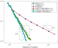
(a) a posteriori error estimation

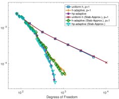
(b) approximate error in energy norm

Figure 1: Error estimates for different families of discrete solutions (Tresca-friction case).

  

\begin{overpic}[trim=796.67715pt 210.55038pt 711.3189pt 145.10905pt,clip,width=142.26378pt,keepaspectratio]{Diri_Stab_approx_h-adaptive_GLeL_theta3_delta5_h_reg4_p_reg2_mesh20_mesh.jpg} \put(8.5,10.5){ \includegraphics[trim=796.67715pt 210.55038pt 711.3189pt 145.10905pt,clip,width=113.81102pt,keepaspectratio]{Diri_Stab_approx_h-adaptive_GLeL_theta3_delta5_h_reg4_p_reg2_mesh10_mesh.jpg} } \end{overpic}

(a) $h$-adaptive

\begin{overpic}[trim=796.67715pt 210.55038pt 711.3189pt 145.10905pt,clip,width=142.26378pt,keepaspectratio]{{Diri_Stab_approx_hp-adaptive_GLeL_theta3.3_delta5_h_reg4_p_reg2_mesh20_mesh}.jpg} \put(8.5,10.5){ \includegraphics[trim=796.67715pt 210.55038pt 711.3189pt 145.10905pt,clip,width=113.81102pt,keepaspectratio]{{Diri_Stab_approx_hp-adaptive_GLeL_theta3.3_delta5_h_reg4_p_reg2_mesh10_mesh}.jpg} } \end{overpic}

(b) $hp$-adaptive

Figure 2: Adaptively generated meshes (Tresca-friction case), mesh nr. 10 (inner), nr. 20 (outer).

​

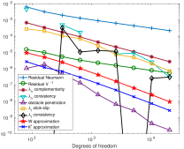
(a) uniform $h$-version with $p=1$

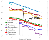
(b) $h$-adaptive with $p=1$

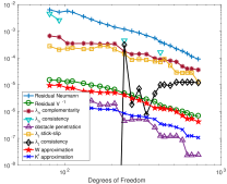
(c) $hp$-adaptive

Figure 3: Error contributions of the residual based a posteriori error estimate (Tresca-friction case).

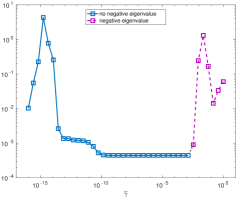
Figure 4: Dependency of the a posteriori error estimate on $\bar{\gamma}$ for a uniform mesh with 256 elements and $p=1$ (Tresca-friction case).

8.2 Two dimensional Coulomb frictional contact problem

For the following numerical experiments taken from [1], see also [26] for FEM results of a very similar problem, the domain is $\Omega=[-\frac{1}{2},\frac{1}{2}]^{2}$ with $\Gamma_{C}=[-\frac{1}{2},\frac{1}{2}]\times\left\{-\frac{1}{2}\right\}$ and $\Gamma_{N}=\partial\Omega\setminus\Gamma_{C}$. Since no Dirichlet boundary is prescribed, the kernel of the Steklov operator consists of the three rigid body motions $\operatorname{ker}(S)=\operatorname{span}\left\{(x_{1},0)^{\top},(0,x_{2})^{\top},(x_{2},-x_{1})^{\top}\right\}$. To obtain a unique solution nevertheless, we fix the point $(0,-1/2)$ as the problem is symmetric. Now, the contact conditions prevent rotations of the body $\Omega$. The material parameters are $E=5$ and $\nu=0.45$, and the Coulomb friction coefficient is $0.3$. The Neumann force is

$$f =\left(\begin{array}[]{c}-10\operatorname{sign}(x_{1})(\frac{1}{2}+x_{2})(\frac{1}{2}-x_{2})\exp(-10(x_{2}+\frac{4}{10})^{2})\\ \frac{7}{8}(\frac{1}{2}+x_{2})(\frac{1}{2}-x_{2})\end{array}\right) \left\{\pm\frac{1}{2}\right\}\times\left[-\frac{1}{2},\frac{1}{2}\right],$$ on

$$f =\left(\begin{array}[]{c}0\\ -\frac{25}{2}(\frac{1}{2}-x_{1})^{2}(\frac{1}{2}+x_{1})^{2}\end{array}\right) \left[-\frac{1}{2},\frac{1}{2}\right]\times\left\{\frac{1}{2}\right\},$$ on

the gap to the obstacle is zero and $\bar{\gamma}=10^{-3}$.

Figure 5 shows the reduction of the error estimate and of the approximate error as in the previous section. The efficiency indices range between 2.6 and 3. The convergence rates are $1.41$ for the uniform $h$-version with $p=1$, (optimal) $1.49$ for the $h$-adaptive scheme with $p=1$ and $\theta=0.4$, and $3.26$ for the $hp$-adaptive scheme with $\theta=0.4$ and $\delta=0.5$. The curve of the a posteriori error estimate for the $hp$-adaptive scheme shows an upwards jump for the duration of two refinements, which is not there in the approximate error curve. That jump is a result of the stick-slip and consistency contribution of $\lambda_{t}$ in the a posteriori error estimate, visuable in Figure 6. That extreme behavior does not seem to be a result of an inaccurate solution of the discrete problem (decreasing the tolerance and changing the iterative solver itself did not affect the upward jumps, and also the residual Neumann contribution of the a posteriori error estimate is not effected), but more a non-conformity problem of the discretization method itself. Enforcing the sign-, box-constraints of $\lambda_{n}$, $\lambda_{t}$, respectively, in the Gauss-Legendre quadrature nodes is very handy for proving convergence rates, but leads to a non-conforming discretization even for $p=1$. If such a constraint violation occurs for the discrete solution, it occurs on a subinterval with positive measure, and is thus picked up strongly by the a posteriori error. These peaks might be avoidable if Bernstein polynomials are used for $\lambda_{hp}$ as suggested in [1].
The adaptively generated meshes show typical refinement pattern and are omitted for brevity.

 

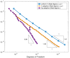
(a) a posteriori error estimation

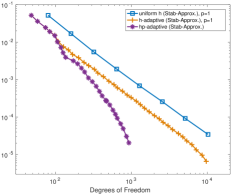
(b) approximate error in energy norm

Figure 5: Error estimates for different families of discrete solutions (Coulomb-friction case).

​

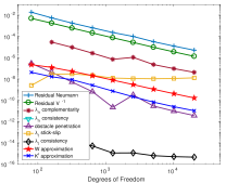
(a) uniform $h$-version with $p=1$

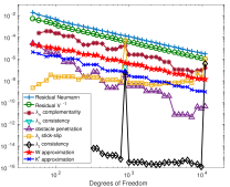
(b) $h$-adaptive with $p=1$

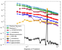
(c) $hp$-adaptive

Figure 6: Error contributions of the residual based a posteriori error estimate (Coulomb-friction case).

8.3 Three dimensional Coulomb frictional contact problem

Let $\Omega=[-1,1]^{3}$, $\Gamma_{C}=[-1,1]^{2}\times\{-1\}$, $\Gamma_{N}=\partial\Omega\setminus\Gamma_{C}$. The remaining data are $\bar{\gamma}=10^{-3}$, $E=5$, $\nu=0.45$, $g=0$, $\mathcal{F}=0.3$ and

$$f =\left(\begin{array}[]{c}-c_{3}\operatorname{sign}(x)(1-z^{2})(1-y^{2})\exp(-c_{4}((z+c_{5})^{2}+y^{2}))\\ 0\\ c_{2}(1-z^{2})(1-y^{2})\end{array}\right) \left\{\pm 1\right\}\times\left[-1,1\right]\times\left[-1,1\right],$$ on

$$f =\left(\begin{array}[]{c}0\\ -c_{3}\operatorname{sign}(y)(1-z^{2})(1-x^{2})\exp(-c_{4}((z+c_{5})^{2}+x^{2}))\\ c_{2}(1-z^{2})(1-x^{2})\end{array}\right) \left[-1,1\right]\times\left\{\pm 1\right\}\times\left[-1,1\right].$$ on

$$f =\left(\begin{array}[]{c}0\\ 0\\ -c_{1}(1-x^{2})(1-y^{2})\exp(-1.5c_{4}(x^{2}+y^{2}))\end{array}\right) \left[-1,1\right]\times\left[-1,1\right]\times\left\{1\right\}$$ on

with $c_{1}=2$, $c_{2}=0.11$, $c_{3}=1.5$, $c_{4}=4$ and $c_{5}=0.5$. The six rigid body motions are removed by limiting the movements of the midpoint of the six faces of the cube according to the symmetry of the domain and of the applied forces. The deformed body with its diamond shaped actual contact set and the negative tangential contact forces are shown in Figure 7.

  

(a) deformed body

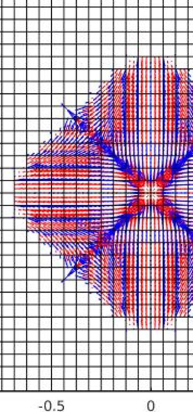
(b) negative tangential contact forces

Figure 7: Discrete solution on uniform mesh with 6144 elements and $p=1$ (3D Coulomb-friction case).

The decay of the a posteriori error estimate and of the approximate error is displayed in Figure 8. The convergence rate of the error and its estimate for the lowest order uniform $h$-version is with $0.75$ w.r.t the degrees of freedom optimal and thus cannot be improved by the corresponding $h$-adaptive method. The $h$-adaptive method with $p=2$ achieves an experimental convergence rate of $0.9$ due to the inability of resolving the free boundary which goes diagonally though the boundary elements by isotropic refinements. The best convergence rate of $1.46$ is obtained with the $hp$-adaptive scheme. Again the isotropic refinement strategy limits the order of convergence, see e.g. [2, 3] for the same observation in a 2d obstacle problem with FEM.

  

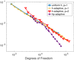
(a) a posteriori error estimation

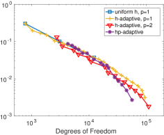
(b) approximate error in energy norm

Figure 8: Error estimates for different families of discrete solutions (3D Coulomb-friction case).

The individual contributions of the a posteriori error estimate are depicted in Figure 9. Once again the dominant source of error is the classical residual error contribution. Equally important is the violation of the stick-slip condition for the $h$-adaptive scheme with $p=2$ and the $hp$-adaptive scheme.

​

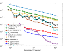
(a) $h$-adaptive with $p=1$

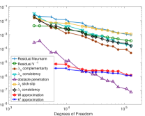
(b) $h$-adaptive with $p=2$

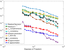
(c) $hp$-adaptive

Figure 9: Error contributions of the residual based a posteriori error estimate (3D Coulomb-friction case).

All three types of adaptive scheme identify the free boundary and perform mesh refinements towards it, c.f. Figure 10. Additionally, the $hp$-meshes show an increase in the polynomial degree away from the free boundary.

​

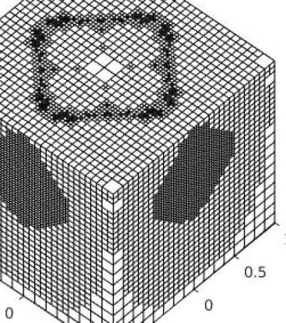
(a) $h$-adaptive with $p=1$

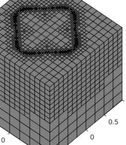
(b) $h$-adaptive with $p=2$

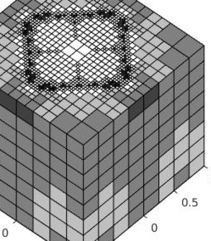
(c) $hp$-adaptive

Figure 10: Adaptively generated meshes (3D Coulomb-friction case).

References

- Banz et al. [2017] L. Banz, H. Gimperlein, A. Issaoui, E.P. Stephan, Stabilized mixed -BEM for frictional contact problems in linear elasticity, Numer. Math. 135 (2017) 217–263.
- Banz and Schröder [2015] L. Banz, A. Schröder, Biorthogonal basis functions in hp-adaptive FEM for elliptic obstacle problems, Comput. Math. Appl. 70 (2015) 1721–1742.
- Banz and Stephan [2014a] L. Banz, E.P. Stephan, A posteriori error estimates of -adaptive IPDG-FEM for elliptic obstacle problems, Appl. Numer. Math. 76 (2014a) 76–92.
- Banz and Stephan [2014b] L. Banz, E.P. Stephan, hp-adaptive IPDG/TDG-FEM for parabolic obstacle problems, Comput. Math. Appl. 67 (2014b) 712–731.
- Banz and Stephan [2015] L. Banz, E.P. Stephan, On -adaptive BEM for frictional contact problems in linear elasticity, Comput. Math. Appl. 69 (2015) 559–581.
- Barbosa and Hughes [1991] H. Barbosa, T. Hughes, The finite element method with the Lagrange multipliers on the boundary: circumventing the Babuška-Brezzi condition, Comput. Methods Appl.Mech.Engrg. 85 (1991) 109–128.
- Barbosa and Hughes [1992] H. Barbosa, T. Hughes, Circumventing the Babuška-Brezzi condition in mixed finite element approximations of elliptic variational inequalities, Comput. Methods Appl.Mech.Engrg. 97 (1992) 193–210.
- Bartels and Carstensen [2004] S. Bartels, C. Carstensen, Averaging techniques yield reliable a posteriori finite element error control for obstacle problems, Numer. Math. 99 (2004) 225–249.
- Bernardi and Maday [1992] C. Bernardi, Y. Maday, Polynomial interpolation results in Sobolev spaces, J. Comput. Appl. Math. 43 (1992) 53–80.
- Biermann et al. [2013] D. Biermann, H. Blum, I. Iovkov, N. Klein, A. Rademacher, F.T. Suttmeier, Stabilization techniques and a posteriori error estimates for the obstacle problem, Appl. Math. Sci. 7 (2013) 6329–6346.
- Boffi et al. [2013] D. Boffi, F. Brezzi, M. Fortin, Mixed Finite Element Methods and Applications, Springer, 2013.
- Carstensen et al. [2001] C. Carstensen, M. Maischak, E.P. Stephan, A posteriori error estimate and h-adaptive algorithm on surfaces for symm’s integral equation, Numer. Math. 90 (2001) 197–213.
- Chernov [2006] A. Chernov, Nonconforming boundary elements and finite elements for interface and contact problems with friction - hp-version for mortar, penalty and Nitsche’s methods, Ph.D. thesis, Universität Hannover, 2006.
- Costabel [1988] M. Costabel, Boundary integral operators on Lipschitz domains: Elementary results, SIAM J. Math. Anal. 19 (1988) 613–626.
- Gwinner [2009] J. Gwinner, On the p-version approximation in the boundary element method for a variational inequality of the second kind modelling unilateral contact and given friction, Appl. Numer. Math. 59 (2009) 2774–2784.
- Gwinner [2013] J. Gwinner, hp-FEM convergence for unilateral contact problems with Tresca friction in plane linear elastostatics, J. Comput. Appl. Math. 254 (2013) 175–184.
- Gwinner and Stephan [1993] J. Gwinner, E.P. Stephan, A boundary element procedure for contact problems in plane linear elastostatics, Modélisation mathématique et analyse numérique 27 (1993) 457–480.
- Han [1994] H. Han, The boundary integro-differential equations of three-dimensional neumann problem in linear elasticity, Numer. Math. 68 (1994) 269–281.
- Heuer [2001] N. Heuer, Additive Schwarz method for the -version of the boundary element method for the single layer potential operator on a plane screen, Numer. Math. 88 (2001) 485–511.
- Hild and Laborde [2002] P. Hild, P. Laborde, Quadratic finite element methods for unilateral contact problems., Appl. Numer. Math. 41 (2002) 401–421.
- Hild and Lleras [2009] P. Hild, V. Lleras, Residual error estimators for Coulomb friction, SIAM J. Numer. Anal. 47 (2009) 3550–3583.
- Hild and Renard [2010] P. Hild, Y. Renard, A stabilized Lagrange multiplier method for the finite element approximation of contact problems in elastostatics, Numer. Math. 115 (2010) 101–129.
- Hlaváček et al. [1988] I. Hlaváček, J. Haslinger, J. Nečas, J. Lovíšek, Solution of variational inequalities in mechanics, Applied Mathematical Sciences, 66. New York etc.: Springer-Verlag, 1988.
- Houston and Süli [2005] P. Houston, E. Süli, A note on the design of hp-adaptive finite element methods for elliptic partial differential equations, Comput. Methods Appl. Mech. Engrg. 194 (2005) 229–243.
- Hüeber et al. [2005] S. Hüeber, A. Matei, B. Wohlmuth, A mixed variational formulation and an optimal a priori error estimate for a frictional contact problem in elasto-piezoelectricity, Bulletin mathématique de la Société des Sciences Mathématiques de Roumanie (2005) 209–232.
- Hüeber and Wohlmuth [2012] S. Hüeber, B. Wohlmuth, Equilibration techniques for solving contact problems with Coulomb friction, Comput. Methods Appl. Mech. Engrg. 205 (2012) 29–45.
- Kikuchi and Oden [1988] N. Kikuchi, J. Oden, Contact problems in elasticity: a study of variational inequalities and finite element methods, volume 8, Society for Industrial Mathematics, 1988.
- Kleiber and Borkowski [1998] M. Kleiber, A. Borkowski, Handbook of computational solid mechanics: survey and comparison of contemporary methods, Springer, 1998.
- Krebs and Stephan [2007] A. Krebs, E.P. Stephan, A p-version finite element method for nonlinear elliptic variational inequalities in 2D, Numer. Math. 105 (2007) 457–480.
- Maischak and Stephan [2005] M. Maischak, E.P. Stephan, Adaptive hp-versions of BEM for Signorini problems, Appl. Numer. Math. 54 (2005) 425–449.
- Maischak and Stephan [2007] M. Maischak, E.P. Stephan, Adaptive hp-versions of boundary element methods for elastic contact problems, Comput. Mech. 39 (2007) 597–607.
- Ovcharova and Banz [2017] N. Ovcharova, L. Banz, Coupling regularization and adaptive -bem for the solution of a delamination problem, Numer. Math. 137 (2017) 303–337.
- Schröder [2011] A. Schröder, Mixed finite element methods of higher-order for model contact problems, SIAM J. Numer. Anal. 49 (2011) 2323–2339.
- Schröder [2012] A. Schröder, A posteriori error estimates of higher-order finite elements for frictional contact problems, Comput. Methods Appl. Mech. Engrg. 249 (2012) 151–157.
- Steinbach [2008] O. Steinbach, Numerical Approximation Methods for Elliptic Boundary Value Problems. Finite and Boundary Elements, Springer, 2008.
- Veeser [2001] A. Veeser, Efficient and reliable a posteriori error estimators for elliptic obstacle problems, SIAM J. Numer. Anal. 39 (2001) 146–167.
- Wohlmuth [2011] B. Wohlmuth, Variationally consistent discretization schemes and numerical algorithms for contact problems, Acta Numer. 20 (2011) 569–734.