Massively scalable Sinkhorn distances via the Nyström method

Abstract

The Sinkhorn “distance,” a variant of the Wasserstein distance with entropic regularization, is an increasingly popular tool in machine learning and statistical inference. However, the time and memory requirements of standard algorithms for computing this distance grow quadratically with the size of the data, making them prohibitively expensive on massive data sets. In this work, we show that this challenge is surprisingly easy to circumvent: combining two simple techniques—the Nyström method and Sinkhorn scaling—provably yields an accurate approximation of the Sinkhorn distance with significantly lower time and memory requirements than other approaches. We prove our results via new, explicit analyses of the Nyström method and of the stability properties of Sinkhorn scaling. We validate our claims experimentally by showing that our approach easily computes Sinkhorn distances on data sets hundreds of times larger than can be handled by other techniques.

1 Introduction

Optimal transport is a fundamental notion in probability theory and geometry (Villani, 2008), which has recently attracted a great deal of interest in the machine learning community as a tool for image recognition (Li et al., 2013; Rubner et al., 2000), domain adaptation (Courty et al., 2017, 2014), and generative modeling (Bousquet et al., 2017; Arjovsky et al., 2017; Genevay et al., 2016), among many other applications (see, e.g., Peyré and Cuturi, 2017; Kolouri et al., 2017).

The growth of this field has been fueled in part by computational advances, many of them stemming from an influential proposal of Cuturi (2013) to modify the definition of optimal transport to include an entropic penalty. The resulting quantity, which Cuturi (2013) called the Sinkhorn “distance” after Sinkhorn (1967), is significantly faster to compute than its unregularized counterpart. Though originally attractive purely for computational reasons, the Sinkhorn distance has since become an object of study in its own right because it appears to possess better statistical properties than the unregularized distance both in theory and in practice (Genevay et al., 2018; Montavon et al., 2016; Peyré and Cuturi, 2017; Schiebinger et al., 2019; Rigollet and Weed, 2018). Computing this distance as quickly as possible has therefore become an area of active study.

We briefly recall the setting. Let $\mathbf{p}$ and $\mathbf{q}$ be probability distributions supported on at most $n$ points in $\mathbb{R}^{d}$. We denote by $\mathcal{M}(\mathbf{p},\mathbf{q})$ the set of all couplings between $\mathbf{p}$ and $\mathbf{q}$, and for any $P\in\mathcal{M}(\mathbf{p},\mathbf{q})$, we denote by $H(P)$ its Shannon entropy. (See Section 2.1 for full definitions.) The Sinkhorn distance between $\mathbf{p}$ and $\mathbf{q}$ is defined as

$$W_{\eta}(\mathbf{p},\mathbf{q}):=\min_{P\in\mathcal{M}(\mathbf{p},\mathbf{q})}\sum_{ij}P_{ij}\|x_{i}-x_{j}\|_{2}^{2}-\eta^{-1}H(P)\,,$$ (1)

for a parameter $\eta>0$. We stress that we use the squared Euclidean cost in our formulation of the Sinkhorn distance. This choice of cost—which in the unregularized case corresponds to what is called the $2$-Wasserstein distance (Villani, 2008)—is essential to our results, and we do not consider other costs here. The squared Euclidean cost is among the most common in applications (Schiebinger et al., 2019; Genevay et al., 2018; Courty et al., 2017; Forrow et al., 2018; Bousquet et al., 2017).

Many algorithms to compute $W_{\eta}(\mathbf{p},\mathbf{q})$ are known. Cuturi (2013) showed that a simple iterative procedure known as Sinkhorn’s algorithm had very fast performance in practice, and later experimental work has shown that greedy and stochastic versions of Sinkhorn’s algorithm perform even better in certain settings (Genevay et al., 2016; Altschuler et al., 2017). These algorithms are notable for their versatility: they provably succeed for any bounded, nonnegative cost. On the other hand, these algorithms are based on matrix manipulations involving the $n\times n$ cost matrix $C$, so their running times and memory requirements inevitably scale with $n^{2}$. In experiments, Cuturi (2013) and Genevay et al. (2016) showed that these algorithms could reliably be run on problems of size $n\approx 10^{4}$.

Another line of work has focused on obtaining better running times when the cost matrix has special structure. A preeminent example is due to Solomon et al. (2015), who focus on the Wasserstein distance on a compact Riemannian manifold, and show that an approximation to the entropic regularized Wasserstein distance can be obtained by repeated convolution with the heat kernel on the domain. Solomon et al. (2015) also establish that for data supported on a grid in $\mathbb{R}^{d}$, significant speedups are possible by decomposing the cost matrix into “slices” along each dimension (see Peyré and Cuturi, 2017, Remark 4.17). While this approach allowed Sinkhorn distances to be computed on significantly larger problems ($n\approx 10^{8}$), it does not extend to non-grid settings. Other proposals include using random sampling of auxiliary points to approximate semi-discrete costs (Tenetov et al., 2018) or performing a Taylor expansion of the kernel matrix in the case of the squared Euclidean cost (Altschuler et al., 2018). These approximations both focus on the $\eta\to\infty$ regime, when the regularization term in (1) is very small, and do not apply to the moderately regularized case $\eta=O(1)$ typically used in practice. Moreover, the running time of these algorithms scales exponentially in the ambient dimension, which can be very large in applications.

1.1 Our contributions

We show that a simple algorithm can be used to approximate $W_{\eta}(\mathbf{p},\mathbf{q})$ quickly on massive data sets. Our algorithm uses only known tools, but we give novel theoretical guarantees that allow us to show that the Nyström method combined with Sinkhorn scaling provably yields a valid approximation algorithm for the Sinkhorn distance at a fraction of the running time of other approaches.

We establish two theoretical results of independent interest: (i) New Nyström approximation results showing that instance-adaptive low-rank approximations to Gaussian kernel matrices can be found for data lying on a low-dimensional manifold (Section 3). (ii) New stability results about Sinkhorn projections, establishing that a sufficiently good approximation to the cost matrix can be used (Section 4).

1.2 Prior work

Computing the Sinkhorn distance efficiently is a well studied problem in a number of communities. The Sinkhorn distance is so named because, as was pointed out by Cuturi (2013), there is an extremely simple iterative algorithm due to Sinkhorn (1967) which converges quickly to a solution to (1). This algorithm, which we call Sinkhorn scaling, works very well in practice and can be implemented using only matrix-vector products, which makes it easily parallelizable. Sinkhorn scaling has been analyzed many times (Franklin and Lorenz, 1989; Linial et al., 1998; Kalantari et al., 2008; Altschuler et al., 2017; Dvurechensky et al., 2018), and forms the basis for the first algorithms for the unregularized optimal transport problem that run in time nearly linear in the size of the cost matrix (Altschuler et al., 2017; Dvurechensky et al., 2018). Greedy and stochastic algorithms related to Sinkhorn scaling with better empirical performance have also been explored (Genevay et al., 2016; Altschuler et al., 2017). Another influential technique, due to Solomon et al. (2015), exploits the fact that, when the distributions are supported on a grid, Sinkhorn scaling performs extremely quickly by decomposing the cost matrix along lower-dimensional slices.

Other algorithms have sought to solve (1) by bypassing Sinkhorn scaling entirely. Blanchet et al. (2018) proposed to solve (1) directly using second-order methods based on fast Laplacian solvers (Cohen et al., 2017; Allen-Zhu et al., 2017). Blanchet et al. (2018) and Quanrud (2019) have noted a connection to packing linear programs, which can also be exploited to yield near-linear time algorithms for unregularized transport distances.

Our main algorithm relies on constructing a low-rank approximation of a Gaussian kernel matrix from a small subset of its columns and rows. Computing such approximations is a problem with an extensive literature in machine learning, where it has been studied under many different names, e.g., Nyström method (Williams and Seeger, 2001), sparse greedy approximations (Smola and Schölkopf, 2000), incomplete Cholesky decomposition (Fine and Scheinberg, 2001), Gram-Schmidt orthonormalization (Shawe-Taylor and Cristianini, 2004) or CUR matrix decompositions (Mahoney and Drineas, 2009). The approximation properties of these algorithms are now well understood (Mahoney and Drineas, 2009; Gittens, 2011; Bach, 2013; Alaoui and Mahoney, 2015); however, in this work, we require significantly more accurate bounds than are available from existing results as well as adaptive bounds for low-dimensional data. To establish these guarantees, we follow an approach based on approximation theory (see, e.g., Rieger and Zwicknagl, 2010; Wendland, 2004; Belkin, 2018), which consists of analyzing interpolation operators for the reproducing kernel Hilbert space corresponding to the Gaussian kernel.

Finally, this paper adds to recent work proposing the use of low-rank approximation for Sinkhorn scaling (Altschuler et al., 2018; Tenetov et al., 2018). We improve upon those papers in several ways. First, although we also exploit the idea of a low-rank approximation to the kernel matrix, we do so in a more sophisticated way that allows for automatic adaptivity to data with low-dimensional structure. These new approximation results are the key to our adaptive algorithm, and this yields a significant improvement in practice. Second, the analyses of Altschuler et al. (2018) and Tenetov et al. (2018) only yield an approximation to $W_{\eta}(\mathbf{p},\mathbf{q})$ when $\eta\to\infty$. In the moderately regularized case when $\eta=O(1)$, which is typically used in practice, neither the work of Altschuler et al. (2018) nor of Tenetov et al. (2018) yields a rigorous error guarantee.

1.3 Outline of paper

Section 2 recalls preliminaries, and then formally states our main result and gives pseudocode for our proposed algorithm. The core of our theoretical analysis is in Sections 3 and 4. Section 3 presents our new results for Nyström approximation of Gaussian kernel matrices and Section 4 presents our new stability results for Sinkhorn scaling. Section 5 then puts these results together to conclude a proof for our main result (Theorem 1). Finally, Section 6 contains experimental results showing that our proposed algorithm outperforms state-of-the-art methods. The appendix contains proofs of several lemmas that are deferred for brevity of the main text.

2 Main result

2.1 Preliminaries and notation

Problem setup.

Throughout, $\mathbf{p}$ and $\mathbf{q}$ are two probability distributions supported on a set $X:=\{x_{1},\dots,x_{n}\}$ of points in $\mathbb{R}^{d}$, with $\|x_{i}\|_{2}\leqslant R$ for all $i\in[n]:=\{1,\dots,n\}$. We define the cost matrix $C\in\mathbb{R}^{n\times n}$ by $C_{ij}=\|x_{i}-x_{j}\|_{2}^{2}$. We identify $\mathbf{p}$ and $\mathbf{q}$ with vectors in the simplex $\Delta_{n}:=\{v\in\mathbb{R}_{\geqslant 0}^{n}:\sum_{i=1}^{n}v_{i}=1\}$ whose entries denote the weight each distribution gives to the points of $X$. We denote by $\mathcal{M}(\mathbf{p},\mathbf{q})$ the set of couplings between $\mathbf{p}$ and $\mathbf{q}$, identified with the set of $P\in\mathbb{R}_{\geqslant 0}^{n\times n}$ satisfying $P\mathbf{1}=\mathbf{p}$ and $P^{\top}\mathbf{1}=\mathbf{q}$, where $\mathbf{1}$ denotes the all-ones vector in $\mathbb{R}^{n}$. The Shannon entropy of a non-negative matrix $P\in\mathbb{R}_{\geqslant 0}^{n\times n}$ is denoted $H(P):=\sum_{ij}P_{ij}\log\tfrac{1}{P_{ij}}$, where we adopt the standard convention that $0\log\tfrac{1}{0}=0$.

Our goal is to approximate the Sinkhorn distance with parameter $\eta>0$:

$$W_{\eta}(\mathbf{p},\mathbf{q}):=\min_{P\in\mathcal{M}(\mathbf{p},\mathbf{q})}\sum_{ij}P_{ij}\|x_{i}-x_{j}\|_{2}^{2}-\eta^{-1}H(P)$$

to some additive accuracy $\varepsilon>0$. By strict convexity, this optimization problem has a unique minimizer, which we denote henceforth by $P^{\eta}$. For shorthand, in the sequel we write

$$V_{M}(P):=\langle M,P\rangle-\eta^{-1}H(P),$$

for a matrix $M\in\mathbb{R}^{n\times n}$. In particular, we have $W_{\eta}(\mathbf{p},\mathbf{q})=\min_{P\in\mathcal{M}(\mathbf{p},\mathbf{q})}V_{C}(P)$. For the purpose of simplifying some bounds, we assume throughout that $n\geqslant 2$, $\eta\in[1,n]$, $R\geqslant 1$, $\varepsilon\leqslant 1$.

Sinkhorn scaling.

Our approach is based on Sinkhorn scaling, an algorithm due to Sinkhorn (1967) and popularized for optimal transport by Cuturi (2013). We recall the following fundamental definition.

Definition 1.

Given $\mathbf{p},\mathbf{q}\in\Delta_{n}$ and $K\in\mathbb{R}^{n\times n}$ with positive entries, the Sinkhorn projection $\Pi^{\mathcal{S}}_{\mathcal{M}(\mathbf{p},\mathbf{q})}(K)$ of $K$ onto $\mathcal{M}(\mathbf{p},\mathbf{q})$ is the unique matrix in $\mathcal{M}(\mathbf{p},\mathbf{q})$ of the form $D_{1}KD_{2}$ for positive diagonal matrices $D_{1}$ and $D_{2}$.

Since $\mathbf{p}$ and $\mathbf{q}$ remain fixed throughout, we abbreviate $\Pi^{\mathcal{S}}_{\mathcal{M}(\mathbf{p},\mathbf{q})}$ by $\Pi^{\mathcal{S}}$ except when we want to make the feasible set $\mathcal{M}(\mathbf{p},\mathbf{q})$ explicit.

Proposition 1 (Wilson, 1969).

Let $K$ have strictly positive entries, and let $\log K$ be the matrix defined by $(\log K)_{ij}:=\log(K_{ij})$. Then

$$\Pi^{\mathcal{S}}_{\mathcal{M}(\mathbf{p},\mathbf{q})}(K)=\operatorname*{argmin}_{P\in\mathcal{M}(\mathbf{p},\mathbf{q})}\langle-\log K,P\rangle-H(P)\,.$$

Note that the strict convexity of $-H(P)$ and the compactness of $\mathcal{M}(\mathbf{p},\mathbf{q})$ implies that the minimizer exists and is unique.

This yields the following simple but key connection between Sinkhorn distances and Sinkhorn scaling.

Corollary 1.

$$P^{\eta}=\Pi^{\mathcal{S}}_{\mathcal{M}(\mathbf{p},\mathbf{q})}(K)\,,$$

where $K$ is defined by $K_{ij}=e^{-\eta C_{ij}}$.

Sinkhorn (1967) proposed to find $\Pi^{\mathcal{S}}(K)$ by alternately renormalizing the rows and columns of $K$. This well known algorithm has excellent performance in practice, is simple to implement, and is easily parallelizable since it can be written entirely in terms of matrix-vector products (Peyré and Cuturi, 2017, Section 4.2). Pseudocode for the version of the algorithm we use can be found in Appendix A.1.

Notation.

We define the probability simplices $\Delta_{n}:=\{p\in\mathbb{R}_{\geqslant 0}^{n}:p^{\top}\mathbf{1}=1\}$ and $\Delta_{n\times n}:=\{P\in\mathbb{R}_{\geqslant 0}^{n\times n}:\mathbf{1}^{\top}P\mathbf{1}=1\}$. Elements of $\Delta_{n\times n}$ will be called joint distributions. The Kullback-Leibler divergence between two joint distributions $P$ and $Q$ is $\mathsf{KL}(P\|Q):=\sum_{ij}P_{ij}\log\tfrac{P_{ij}}{Q_{ij}}$.

Throughout the paper, all matrix exponentials and logarithms will be taken entrywise, i.e., $(e^{A})_{ij}:=e^{A_{ij}}$ and $(\log A)_{ij}:=\log A_{ij}$ for $A\in\mathbb{R}^{n\times n}$.

Given a matrix $A$, we denote by $\|A\|_{\mathrm{op}}$ its operator norm (i.e., largest singular value), by $\|A\|_{*}$ its nuclear norm (i.e., the sum of its singular values), by $\|A\|_{1}$ its entrywise $\ell_{1}$ norm (i.e., $\|A\|_{1}:=\sum_{ij}|A_{ij}|$), and by $\|A\|_{\infty}$ its entrywise $\ell_{\infty}$ norm (i.e., $\|A\|_{\infty}:=\max_{ij}|A_{ij}|$). We abbreviate “positive semidefinite” by “PSD.”

The notation $f=O(g)$ means that $f\leqslant Cg$ for some universal constant $C$, and $g=\Omega(f)$ means $f=O(g)$. The notation $\tilde{O}(\cdot)$ omits polylogarithmic factors depending on $R$, $\eta$, $n$, and $\varepsilon$.

2.2 Main result and proposed algorithm

Pseudocode for our proposed algorithm is given in Algorithm 1. Nys-Sink (pronounced “nice sink”) computes a low-rank Nyström approximation of the kernel matrix via a column sampling procedure. While explicit low-rank approximations of Gaussian kernel matrices can also be obtained via Taylor explansion (Cotter et al., 2011), our approach automatically adapts to the properties of the data set, leading to much better performance in practice.

As noted in Section 1, the Nyström method constructs a low-rank approximation to a Gaussian kernel matrix $K=e^{-\eta C}$ based on a small number of its columns. In order to design an efficient algorithm, we aim to construct such an approximation with the smallest possible rank. The key quantity for understanding the error of this algorithm is the so-called effective dimension (also sometimes called the “degrees of freedom”) of the kernel $K$ (Friedman et al., 2001; Zhang, 2005; Musco and Musco, 2017).

Definition 2.

Let $\lambda_{j}(K)$ denote the $j$th largest eigenvalue of $K$ (with multiplicity). Then the effective dimension of $K$ at level $\tau>0$ is

$$d_{\textrm{eff}}(\tau):=\sum_{j=1}^{n}\frac{\lambda_{j}(K)}{\lambda_{j}(K)+\tau n}.$$ (2)

The effective dimension $d_{\textrm{eff}}(\tau)$ indicates how large the rank of an approximation $\tilde{K}$ to $K$ must be in order to obtain the guarantee $\|\tilde{K}-K\|_{\mathrm{op}}\leqslant\tau n$. As we will show in Section 5, below, it will suffice for our application to obtain an approximate kernel $\tilde{K}$ satisfying $\|\tilde{K}-K\|_{\mathrm{op}}\leqslant\tfrac{\varepsilon^{\prime}}{2}e^{-4\eta R^{2}}$, where $\varepsilon^{\prime}=\tilde{O}(\varepsilon R^{-2})$. We are therefore motivated to define the following quantity, which informally captures the smallest possible rank of an approximation of this quality.

Definition 3.

Given $X=\{x_{1},\dots,x_{n}\}\subseteq\mathbb{R}^{d}$ with $\|x_{i}\|_{2}\leqslant R$ for all $i\in[n]$, $\eta>0$, and $\varepsilon^{\prime}\in(0,1)$, the approximation rank is

$$r^{*}(X,\eta,\varepsilon^{\prime}):=d_{\textrm{eff}}\left(\tfrac{\varepsilon^{\prime}}{2n}e^{-4\eta R^{2}}\right)$$

where $d_{\textrm{eff}}(\cdot)$ is the effective rank for the kernel matrix $K:=e^{-\eta C}$.

As we show below, we adaptively construct an approximate kernel $\tilde{K}$ whose rank is at most a logarithmic factor bigger than $r^{*}(X,\eta,\varepsilon^{\prime})$ with high probability. We also give concrete bounds on $r^{*}(X,\eta,\varepsilon^{\prime})$ below.

Our proposed algorithm makes use of several subroutines. The AdaptiveNyström procedure in line 4 combines an algorithm of Musco and Musco (2017) with a doubling trick that enables automatic adaptivity; this is described in Section 3. It outputs the approximate kernel $\tilde{K}$ and its rank $r$. The Sinkhorn procedure in line 5 is the Sinkhorn scaling algorithm for projecting $\tilde{K}$ onto $\mathcal{M}(\mathbf{p},\mathbf{q})$, pseudocode for which can be found in Appendix A.1. We use a variant of the standard algorithm, which returns both the scaling matrices and an approximation of the cost of an optimal solution. The Round procedure in line 6 is Algorithm 2 of Altschuler et al. (2017); for completeness, pseudocode can be found here in Appendix A.2.

We emphasize that neither $D_{1}\tilde{K}D_{2}$ nor $\hat{P}$ (which is of the form $D_{1}^{\prime}\tilde{K}D_{2}^{\prime}+vw^{T}$ for diagonal matrices $D_{1}^{\prime},D_{2}^{\prime}$ and vectors $v,w$) are ever represented explicitly, since this would take $\Omega(n^{2})$ time. Instead, we maintain these matrices in low-rank factorized forms. This enables Algorithm 1 to be implemented efficiently in $o(n^{2})$ time, since the procedures Sinkhorn and Round can both be implemented such that they depend on $\tilde{K}$ only through matrix-vector multiplications with $\tilde{K}$. Moreover, we also emphasize that all steps of Algorithm 1 are easily parallelizable since they can be re-written in terms of matrix-vector multiplications.

We note also that although the present paper focuses specifically on the squared Euclidean cost $c(x_{i},x_{j})=\|x_{i}-x_{j}\|_{2}^{2}$ (corresponding to the $2$-Wasserstein case of optimal transport pervasively used in applications; see intro), our algorithm Nys-Sink readily extends to other cases of optimal transport. Indeed, since the Nyström method works not only for Gaussian kernel matrices $K_{ij}=e^{-\eta\|x_{i}-x_{j}\|_{2}^{2}}$, but in fact more generally for any PSD kernel matrix, our algorithm can be used on any optimal transport instance for which the corresponding kernel matrix $K_{ij}=e^{-\eta c(x_{i},x_{j})}$ is PSD.

1:$X=\{x_{1},\dots,x_{n}\}\subseteq\mathbb{R}^{d}$, $\mathbf{p},\mathbf{q}\in\Delta_{n}$, $\varepsilon,\eta>0$

2:$\hat{P}\in\mathcal{M}(\mathbf{p},\mathbf{q})$, $\hat{W}\in\mathbb{R}$, $r\in\mathbb{N}$

3:$\varepsilon^{\prime}\leftarrow\min(1,\tfrac{\varepsilon\eta}{50(4R^{2}\eta+\log\tfrac{n}{\eta\varepsilon})})$

4:$(\tilde{K},r)\leftarrow\textsc{AdaptiveNystr\"{o}m}(X,\eta,\tfrac{\varepsilon^{\prime}}{2}e^{-4\eta R^{2}})$ $\triangleright$ Compute low-rank approximation

5:$(D_{1},D_{2},\hat{W})\leftarrow\textsc{Sinkhorn}(\tilde{K},\mathbf{p},\mathbf{q},\varepsilon^{\prime})$ $\triangleright$ Approximate Sinkhorn projection and cost

6:$\hat{P}\leftarrow\textsc{Round}(D_{1}\tilde{K}D_{2},\mathbf{p},\mathbf{q})$ $\triangleright$ Round to feasible set

7:return $\hat{P}$, $\hat{W}$

Algorithm 1 Nys-Sink

Our main result is the following.

Theorem 1.

Let $\varepsilon,\delta\in(0,1)$. Algorithm 1 runs in $\tilde{O}\left(nr\left(r+\tfrac{\eta R^{4}}{\varepsilon}\right)\right)$ time, uses $O(n(r+d))$ space, and returns a feasible matrix $\hat{P}\in\mathcal{M}(\mathbf{p},\mathbf{q})$ in factored form and scalars $\hat{W}\in\mathbb{R}$ and $r\in\mathbb{N}$, where

$$|V_{C}(\hat{P})-W_{\eta}(\mathbf{p},\mathbf{q})| \leqslant\varepsilon,$$ (3a)

$$\mathsf{KL}(\hat{P}\|P^{\eta}) \leqslant\eta\varepsilon,$$ (3b)

$$|\hat{W}-W_{\eta}(\mathbf{p},\mathbf{q})| \leqslant\varepsilon,\,$$ (3c)

and, with probability $$1-\delta$$,

$$r \leqslant c\cdot r^{*}(X,\eta,\varepsilon^{\prime})\log\tfrac{n}{\delta}\,,$$ (3d)

for a universal constant $$c \varepsilon^{\prime}=\tilde{\Omega}(\varepsilon R^{-2})$$ and where .

We note that, while our algorithm is randomized, we obtain a deterministic guarantee that $\hat{P}$ is a good solution. We also note that runtime dependence on the radius $R$—which governs the scale of the problem—is inevitable since we seek an additive guarantee.

Crucially, we show in Section 3 that $r^{*}$—which controls the running time of the algorithm with high probability by (3d)—adapts to the intrinsic dimension of the data. This adaptivity is crucial in applications, where data can have much lower dimension than the ambient space. We informally summarize this behavior in the following theorem.

Theorem 2 (Informal).

1. There exists an universal constant $c>0$ such that, for any $n$ points in a ball of radius $R$ in $\mathbb{R}^{d}$,

   $$r^{*}(X,\eta,\varepsilon^{\prime})\leqslant(c(\eta R^{2}+\log\tfrac{n}{\varepsilon^{\prime}\eta}))^{d}\,.$$

2. For any $k$-dimensional manifold $\Omega$ satisfying certain technical conditions and $\eta>0$, there exists a constant $c_{\Omega,\eta}$ such that for any $n$ points lying on $\Omega$,

   $$r^{*}(X,\eta,\varepsilon^{\prime})\leqslant c_{\Omega,\eta}(\log\tfrac{n}{\varepsilon^{\prime}})^{5k/2}\,.$$

The formal versions of these bounds appear in Section 3. The second bound is significantly better than the first when $k\ll d$, and clearly shows the benefits of an adaptive procedure.

Combining Theorems 1 and 2 yields the following time and space complexity for our algorithm.

Corollary 2 (Informal).

If $X$ consists of $n$ points lying in a ball of radius $R$ in $\mathbb{R}^{d}$, then with high probability Algorithm 1 requires

$$\tilde{O}\left(n\cdot\frac{1}{\varepsilon}\left(c\eta R^{2}+c\log\frac{n}{\varepsilon}\right)^{2d+1}\right)\text{ time and }\tilde{O}\left(n\cdot\left(c\eta R^{2}+c\log\frac{n}{\varepsilon}\right)^{d}\right)\text{ space.}$$

Moreover, if $X$ lies on a $k$-dimensional manifold $\Omega$, then with high probability Algorithm 1 requires

$$\tilde{O}\left(n\cdot\frac{c_{\Omega,\eta}}{\varepsilon}\left(\log\frac{n}{\varepsilon}\right)^{5k}\right)\text{ time and }\tilde{O}\left(n\cdot c_{\Omega,\eta}\left(\log\frac{n}{\varepsilon}\right)^{5k/2}\right)\text{ space.}$$

Altschuler et al. (2017) noted that an approximation to the unregularized optimal transport cost is obtained by taking $\eta=\Theta\left(\varepsilon^{-1}\log n\right)$. Thus it follows that Algorithm 1 computes an additive $\varepsilon$ approximation to the unregularized transport distance in $O\left(n\left(\varepsilon^{-1}R^{2}\log n\right)^{O(d)}\right)$ time with high probability. However, a theoretically better running time for that problem can be obtained by a simple but impractical algorithm based on rounding the input distributions to an $\varepsilon$-net and then running Sinkhorn scaling on the resulting instance.

3 Kernel approximation via the Nyström method

In this section, we describe the algorithm AdaptiveNyström used in line 4 of Algorithm 1 and bound its runtime complexity, space complexity, and error. We first establish basic properties of Nyström approximation and give pseudocode for AdaptiveNyström (Sections 3.1 and 3.2) before stating and proving formal versions of the bounds appearing in Theorem 2 (Sections 3.3 and 3.4).

3.1 Preliminaries: Nyström and error in terms of effective dimension

Given points $X=\{x_{1},\dots,x_{n}\}$ with $\|x_{i}\|_{2}\leqslant R$ for all $i\in[n]$, let $K\in\mathbb{R}^{n\times n}$ denote the matrix with entries $K_{ij}:=k_{\eta}(x_{i},x_{j})$, where $k_{\eta}(x,x^{\prime}):=e^{-\eta\|x-x^{\prime}\|^{2}}$. Note that $k_{\eta}(x,x^{\prime})$ is the Gaussian kernel $e^{-\|x-x^{\prime}\|^{2}/(2\sigma^{2})}$ between points $x$ and $x^{\prime}$ with bandwith parameter $\sigma^{2}=\tfrac{1}{2\eta}$. For $r\in\mathbb{N}$, we consider an approximation of the matrix $K$ that is of the form

$$\widetilde{K}=VA^{-1}V^{\top},$$

where $V\in\mathbb{R}^{n\times r}$ and $A\in\mathbb{R}^{r\times r}$. In particular we will consider the approximation given by the Nyström method which, given a set $X_{r}=\{\widetilde{x}_{1},\dots,\widetilde{x}_{r}\}\subset X$, constructs $V$ and $A$ as:

$$V_{ij}=k_{\eta}(x_{i},\widetilde{x}_{j}),\quad A_{jj^{\prime}}=k_{\eta}(\widetilde{x}_{j},\widetilde{x}^{\prime}_{j}),$$

for $i\in[n]$ and $j,j^{\prime}\in[r]$. Note that the matrix $\widetilde{K}$ is never computed explicitly. Indeed, our proposed Algorithm 1 only depends on $\widetilde{K}$ through computing matrix-vector products $\widetilde{K}v$, where $v\in\mathbb{R}^{n}$, and these can be computed efficiently as

$$\widetilde{K}v=V(L^{-\top}(L^{-1}(V^{\top}v))),$$ (4)

where $L\in\mathbb{R}^{r\times r}$ is the lower triangular matrix satisfying $LL^{\top}=A$ obtained by the Cholesky decomposition of $A$, and where we compute products of the form $L^{-1}v$ (resp. $L^{-\top}v$) by solving the triangular system $Lx=v$ (resp. $L^{\top}x=v$). Once a Cholesky decomposition of $A$ has been obtained—at computational cost $O(r^{3})$—matrix-vector products can therefore be computed in time $O(nr)$.

We now turn to understanding the approximation error of this method. In this paper we will sample the set $X_{r}$ via approximate leverage-score sampling. In particular, we do this via Algorithm 2 of Musco and Musco (2017). The following lemma shows that taking the rank $r$ to be on the order of the effective dimension $d_{\textrm{eff}}(\tau)$ (see Definition 3) is sufficient to guarantee that $\widetilde{K}$ approximates $K$ to within error $\tau$ in operator norm.

Lemma 1.

Let $\tau,\delta>0$. Consider sampling $X_{r}$ from $X$ according to Algorithm 2 of Musco and Musco (2017), for some positive integer $r\geqslant 400d_{\textrm{eff}}(\tau)\log\tfrac{3n}{\delta}.$ Then:

1. Sampling $X_{r}$ and forming the matrices $V$ and $L$ (which define $\tilde{K}$, see (4)) requires $O(nr^{2}+r^{3})$ time and $O(n(r+d))$ space.

2. Computing matrix-vector products with $\tilde{K}$ can be done in time $O(nr)$.

3. With probability at least $1-\delta$, $\|K-\widetilde{K}\|_{\mathrm{op}}\leqslant\tau n$.

Proof.

The result follows directly from Theorem 7 of Musco and Musco (2017) and the fact that $d_{\textrm{eff}}(\tau)\leqslant\textrm{rank}(K)\leqslant n$ for any $\tau\geqslant 0$. ∎

3.2 Adaptive Nyström with doubling trick

Here we give pseudocode for the AdaptiveNyström subroutine in Algorithm 2. The algorithm is based on a simple doubling trick, so that the rank of the approximate kernel can be chosen adaptively. The observation enabling this trick is that given a Nyström approximation $\tilde{K}$ to the actual kernel matrix $K=e^{-\eta\|x_{i}-x_{j}\|_{2}^{2}}$, the entrywise error $\|K-\tilde{K}\|_{\infty}$ of the approximation can be computed exactly in $O(nr^{2})$ time. The reason for this is that (i) the entrywise norm $\|K-\tilde{K}\|_{\max}$ is equal to the maximum entrywise error on the diagonal $\max_{i\in[n]}|K_{ii}-\tilde{K}_{ii}|=1-\min_{i\in[n]}\tilde{K}_{ii}$, proven below in Lemma 2; and (ii) the quantity $1-\min_{i\in[n]}\tilde{K}_{ii}$ is easy to compute quickly.

Below, line 6 in Algorithm 2 denotes the approximate leverage-score sampling scheme of Musco and Musco (2017, Algorithm 2) when applied to the Gaussian kernel matrix $K_{ij}:=e^{-\eta\|x_{i}-x_{j}\|^{2}}$. We note that the BLESS algorithm of Rudi et al. (2018) allows for re-using previously sampled points when doubling the sampling rank. Although this does not affect the asymptotic runtime, it may lead to speedups in practice.

1:$X=\{x_{1},\dots,x_{n}\}\in\mathbb{R}^{d\times n}$, $\eta>0$, $\tau>0$

2:$\tilde{K}\in\mathbb{R}^{n\times n}$, $r\in\mathbb{N}$

3:$\mathsf{err}\leftarrow+\infty$, $r\leftarrow 1$

4:while $\mathsf{err}>\tau$ do

5:     $r\leftarrow 2r$

6:     $\tilde{K}\leftarrow\textsc{Nystr\"{o}m}(X,\eta,r)$

7:     $\mathsf{err}\leftarrow 1-\min_{i\in[n]}\tilde{K}_{ii}$

8:end while

9:return $(\tilde{K},\text{rank}(\tilde{K}))$

Algorithm 2 AdaptiveNyström

Lemma 2.

Let $(\tilde{K},r)$ denote the (random) output of $\textsc{AdaptiveNystr\"{o}m}(X,\eta,\tau)$. Then:

1. $\|K-\tilde{K}\|_{\infty}\leqslant\tau$.

2. The algorithm used $O(nr)$ space and terminated in $O(nr^{2})$ time.

3. There exists a universal constant $c$ such that simultaneously for every $\delta>0$,

   $$\mathbb{P}\Big{(}r\leqslant c\cdot d_{\textrm{eff}}\left(\tfrac{\tau}{n}\right)\log\left(\tfrac{n}{\delta}\right)\Big{)}\geqslant 1-\delta.$$

Proof.

By construction, the Nyström approximation $\tilde{K}$ is a PSD approximation of $K$ in the sense that $K\succeq\tilde{K}\succeq 0$, see e.g., Musco and Musco (2017, Theorem 3). Since Sylvester’s criterion for $2\times 2$ minors guarantees that the maximum modulus entry of a PSD matrix is always achieved on the diagonal, it follows that $\|K-\tilde{K}\|_{\infty}=\max_{i\in[n]}|K_{ii}-\tilde{K}_{ii}|$. Now each $K_{ii}=1$ by definition of $K$, and each $\tilde{K}_{ii}\in[0,1]$ since $K\succeq\tilde{K}\succeq 0$. Therefore we conclude

$$\|K-\tilde{K}\|_{\infty}=1-\min_{i\in[n]}\tilde{K}_{ii}.$$

This implies Item 1. Item 2 follows upon using the space and runtime complexity bounds in Lemma 1 and noting that the final call to Nyström is the dominant for both space and runtime. Item 3 is immediate from Lemma 1 and the fact that $\|K-\tilde{K}\|_{\infty}\leqslant\|K-\tilde{K}\|_{\mathrm{op}}$ (Lemma J). ∎

3.3 General results: data points lie in a ball

In this section we assume no structure on $X$ apart from the fact that $X\subseteq B^{d}_{R}$ where $B^{d}_{R}$ is a ball of radius $R$ in $\mathbb{R}^{d}$ centered around the origin, for some $R>0$ and $d\in\mathbb{N}$. First we characterize the eigenvalues of $K$ in terms of $\eta,d,R$, and then we use this to bound $d_{\textrm{eff}}$.

Theorem 3.

Let $X:=\{x_{1},\dots x_{n}\}\subseteq B_{R}^{d}$, and let $K\in\mathbb{R}^{n\times n}$ be the matrix with entries $K_{ij}:=e^{-\eta\|x_{i}-x_{j}\|^{2}}$. Then:

1. For each $t\in\mathbb{N},t\geqslant(2e)^{d}$, $\lambda_{t+1}(K)\leqslant ne^{-\frac{d}{2e}t^{1/d}\log{d~{}t^{1/d}\over 4e^{2}\eta R^{2}}}$.

2. For each $\tau\in(0,1]$, $d_{\textrm{eff}}(\tau)\leqslant 3\left(6+\frac{41}{d}\eta R^{2}+\frac{3}{d}\log\frac{1}{\tau}\right)^{d}$.

We sketch the proof of Theorem 3 here; details are deferred to Appendix B.5 for brevity of the main text. We begin by recalling the argument of Cotter et al. (2011) that truncating the Taylor expansion of the Gaussian kernel guarantees for each positive integer $T$ the existence of a rank $M_{T}:=\binom{d+T}{T}$ matrix $\tilde{K}_{T}$ satisfying

$$\|K-\tilde{K}_{T}\|_{\infty}\leqslant\frac{(2\eta R^{2})^{T+1}}{(T+1)!}.$$

On the other hand, by the Eckart-Young-Mirsky Theorem,

$$\lambda_{M_{T}+1}=\inf_{\bar{K}_{T}\in\mathbb{R}^{n\times n},\,\text{rank}(\bar{K}_{T})\leqslant M_{T}}\|K-\bar{K}_{T}\|_{\text{op}}.$$

Therefore by combining the above two displays, we conclude that

$$\lambda_{M_{T}+1}\leqslant\|K-\tilde{K}_{T}\|_{\text{op}}\leqslant n\|K-\tilde{K}_{T}\|_{\infty}\leqslant n\frac{(2\eta R^{2})^{T+1}}{(T+1)!}.$$

Proofs of the two claims follow by bounding this quantity. Details are in Appendix B.5.

Theorem 3 characterizes the eigenvalue decay and effective dimension of Gaussian kernel matrices in terms of the dimensionality of the space, with explicit constants and explicit dependence on the width parameter $\eta$ and the radius $R$ of the ball (see Belkin, 2018, for asymptotic results). This yields the following bound on the optimal rank for approximating Gaussian kernel matrices of data lying in a Euclidean ball.

Corollary 3.

Let $\varepsilon^{\prime}\in(0,1)$ and $\eta>0$. If $X$ consists of $n$ points lying in a ball of radius $R$ around the origin in $\mathbb{R}^{d}$, then

$$r^{*}(X,\eta,\varepsilon^{\prime})\leqslant 3\left(6+\frac{53}{d}\eta R^{2}+\frac{3}{d}\log\frac{2n}{\varepsilon^{\prime}}\right)^{d}$$

Proof.

Directly from the explicit bound of Theorem 3 and the definition of $r^{*}(X,\eta,\varepsilon^{\prime})$. ∎

3.4 Adaptivity: data points lie on a low dimensional manifold

In this section we consider $X\subset\Omega\subset\mathbb{R}^{d}$, where $\Omega$ is a low dimensional manifold. In Theorem 4 we give a result about the approximation properties of the Gaussian kernel over manifolds and a bound on the eigenvalue decay and effective dimension of Gaussian kernel matrices. We prove that the effective dimension is logarithmic in the precision parameter $\tau$ to a power depending only on the dimensionality $k$ of the manifold (to be contrasted to the dimensionality of the ambient space $d\gg k$).

Let $\Omega\subset\mathbb{R}^{d}$ be a smooth compact manifold without boundary, and $k<d$. Let $(\Psi_{j},U_{j})_{j\in[T]}$, with $T\in\mathbb{N}$, be an atlas for $\Omega$, where without loss of generality, $(U_{j})_{j}$ are open sets covering $\Omega$, $\Psi_{j}:U_{j}\to B^{k}_{r_{j}}$ are smooth maps with smooth inverses, mapping $U_{j}$ bijectively to $B^{k}_{r_{j}}$, balls of radius $r_{j}$ centered around the origin of $\mathbb{R}^{k}$. We assume the following quantitative control on the smoothness of the atlas.

Assumption 1.

There exists $Q>0$ such that

$$\sup_{u\in B^{k}_{r_{j}}}\|D^{\alpha}\Psi_{j}^{-1}(u)\|\leqslant Q^{|\alpha|},\qquad\alpha\in\mathbb{N}^{k},j\in[T],$$

where $|\alpha|=\sum_{j=1}^{k}\alpha_{j}$ and $D^{\alpha}=\frac{\partial^{|\alpha|}}{\partial u_{1}^{\alpha_{1}}\dots\partial u_{k}^{\alpha_{k}}}$, for $\alpha\in\mathbb{N}^{k}$.

Before stating our result, we need to introduce the following helpful definition. Given $f:\mathbb{R}^{d}\to\mathbb{R}$, and $X=\{x_{1},\dots,x_{n}\}\subset\Omega$, denote by $\widehat{f}_{X}$ the function

$$\widehat{f}_{X}(x):=\sum_{i=1}^{n}c_{i}k_{\eta}(x,x_{i}),\quad c=K^{-1}v_{f},$$

with $v_{f}=(f(x_{1}),\dots,f(x_{n}))$ and $K\in\mathbb{R}^{n\times n}$ the kernel matrix over $X$, i.e. $K_{ij}=k_{\eta}(x_{i},x_{j})$. Note that $\widehat{f}_{X}(x_{i})=f(x_{i})$ by construction (Wendland, 2004). We have the following result.

Theorem 4.

Let $\Omega\subset B_{R}^{d}\subset\mathbb{R}^{d}$ be a smooth compact manifold without boundary satisfying 1. Let $X\subset\Omega$ be a set of cardinality $n\in\mathbb{N}$. Then the following holds

1. Let $h_{X,\Omega}=\sup_{x^{\prime}\in\Omega}\inf_{x\in X}\|x-x^{\prime}\|$. Let $\mathcal{H}$ be the RKHS associated to the Gaussian kernel of a given width. There exist $c,h>0$ not depending on $X,n$, such that, when $h_{X,\Omega}\leqslant h$ the following holds

   $$|f(x)-\widehat{f}_{X}(x)|\leqslant e^{-ch_{X,\Omega}^{-2/5}}\|f\|_{\mathcal{H}},\qquad\forall f\in\mathcal{H},~{}~{}x\in\Omega.$$

2. Let $K$ be the Gaussian kernel matrix associated to $X$. Then there exists a constant $c$ not depending on $X$ or $n$, for which

   $$\lambda_{p+1}(K)\leqslant ne^{-cp^{\frac{2}{5k}}},\qquad\forall p\in[n].$$

3. Let $\tau\in(0,1]$. Let $K$ be the Gaussian kernel matrix associated to $X$ and $d_{\textrm{eff}}(\tau)$ the effective dimension computed on $K$. There exists $c_{1},c_{2}$ not depending on $X$, $n$, or $\tau$, for which

   $$d_{\textrm{eff}}(\tau)\leqslant\left(c_{1}\log\frac{1}{\tau}\right)^{5k/2}+c_{2}.$$

Proof.

First we recall some basic multi-index notation and introduce Sobolev Spaces. When $\alpha\in\mathbb{N}_{0}^{d},x\in\mathbb{R}^{d},g:\mathbb{R}^{d}\to\mathbb{R}$, we write

$$x^{\alpha}=\prod_{i}x_{i}^{\alpha_{i}},~{}~{}|\alpha|=\sum_{i}\alpha_{i},~{}~{}\alpha!=\prod_{i}\alpha_{i}!,~{}~{}D^{\alpha}=\frac{\partial^{|\alpha|}}{\partial x_{1}^{\alpha_{1}}\dots\partial x_{n}^{\alpha_{n}}}.$$

Next, we recall the definition of Sobolev spaces. For $m,p\in\mathbb{N}$ and $B\subseteq\mathbb{R}^{k}$, define the norm $\|\cdot\|_{W^{m}_{p}(B)}$ by

$$\|f\|^{p}_{W^{m}_{p}(B)}=\sum_{|\alpha|\leqslant m}\|D^{\alpha}f\|^{p}_{L^{p}(B)},$$

and the space of $W^{m}_{p}(B)$ as $W^{m}_{p}(B)=\overline{C^{\infty}(B)}^{\|\cdot\|_{W^{m}_{p}(B)}}$.

For any $j\in[T]$, $u\in\mathcal{H}$ we have the following. By O, we have that there exists a constant $C_{d,k,R,r_{j}}$ such that for any $q\geqslant k$,

$$\|u\circ\Psi_{j}^{-1}\|_{W^{q}_{2}(B^{k}_{r_{j}})}\leqslant C_{d,k,R,r_{j}}q^{k}(2qdQ)^{q}\|u\|_{W^{q+(d+1)/2}_{2}(B^{d}_{R})}.$$

Now note that by Theorem 7.5 of Rieger and Zwicknagl (2010) we have that there exists a constant $C_{\eta}$ such that

$$\|u\|_{W^{q+(d+1)/2}_{2}(B^{d}_{R})}\leqslant\|u\|_{W^{q+(d+1)/2}_{2}(\mathbb{R}^{d})}\leqslant(C_{\eta})^{q+(d+1)/2}\left(q+\frac{d+1}{2}\right)^{\frac{q}{2}+\frac{d+1}{4}}\|u\|_{\mathcal{H}}.$$

Then, since $q^{m}\leqslant m^{m}(1+m)^{q}$, for any $q\geqslant 1$, we have

$$\|u\circ\Psi_{j}^{-1}\|_{W^{q}_{2}(B^{k}_{r_{j}})}\leqslant C_{d,k,R,r_{j},Q,\eta}^{q}q^{\frac{3q}{2}}\|u\|_{\mathcal{H}},$$

for a suitable constant $C_{d,k,R,r_{j},Q,\eta}$ depending on $C_{d,k,R,r_{j},Q}$, $C_{\eta}$ and $(d+1)/2$.

In particular we want to study $\|u\|_{L^{\infty}(\Omega)}$, for $u=f-\widehat{f}_{X}$. We have

$$\|u\|_{L^{\infty}(\Omega)}=\sup_{j\in[T]}\|u\|_{L^{\infty}(U_{j})}=\sup_{j\in[T]}\|u\circ\Psi_{j}^{-1}\|_{L^{\infty}(B^{k}_{r_{j}})}.$$

Now for $j\in[T]$, denote by $Z_{j}$ the set $Z_{j}=\{\Psi_{j}(x)|x\in X\cap U_{j}\}$. By construction of $u=f-\widehat{f}_{X}$, we have

$$(u\circ\Psi_{j}^{-1})|_{Z_{j}}=u|_{X\cap U_{j}}=0.$$

Define $h_{Z_{j},B^{k}_{r_{j}}}=\sup_{z\in B^{k}_{r_{j}}}\inf_{z^{\prime}\in Z_{j}}\|z-z^{\prime}\|$. We have established that there exists $C>0$, such that $\|u\circ\Psi_{j}^{-1}\|_{W^{q}_{2}(B^{k}_{r_{j}})}\leqslant C^{q}q^{\frac{3}{2}q}\|u\|_{\mathcal{H}}$, and by construction $(u\circ\Psi_{j})|_{Z_{j}}=0$. We can therefore apply Theorem 3.5 of Rieger and Zwicknagl (2010) to obtain that there exists a $c_{j},h_{j}>0$, for which, when $h_{Z_{j},B^{k}_{r_{j}}}\leqslant h_{j}$, then

$$\|u\circ\Psi_{j}^{-1}\|_{L^{\infty}(B^{k}_{r_{j}})}\leqslant\exp\left(-c_{j}h_{Z_{j},B^{k}_{r_{j}}}^{-2/5}\right)\|u\|_{\mathcal{H}}.$$

Now, denote by $\bar{h}_{S,U}=\sup_{x^{\prime}\in U}\inf_{x\in S}d(x,x^{\prime})$ with $d$ the geodesic distance over the manifold $\Omega$. By applying Theorem 8 of Fuselier and Wright (2012), we have that there exist $C$ and $h_{0}$ not depending on $X$ or $n$ such that, when $\bar{h}_{X,\Omega}\leqslant h_{0}$, the inequality $\bar{h}_{X_{j}\cap U_{j},U_{j}}\leqslant C\bar{h}_{X,\Omega}$ holds for any $j\in[T]$. Moreover, since by Theorem 6 of the same paper $\|x-x^{\prime}\|\leqslant d(x,x^{\prime})\leqslant C_{1}\|x-x^{\prime}\|$, for $C_{1}>1$ and $x,x^{\prime}\in\Omega$, then

$$h_{Z_{j},B^{k}_{r_{j}}}\leqslant\bar{h}_{X_{j}\cap U_{j},U_{j}}\leqslant C\bar{h}_{X,\Omega}\leqslant CC_{1}h_{X,\Omega}.$$

Finally, defining $c_{1}=c(2\max_{j}C_{j})^{-2/5},h=C_{1}^{-1}\min(h_{0},C^{-1}\min_{j}h_{j})$, when $h_{X,\Omega}\leqslant h$,

$$\|f-\widehat{f}_{X}\|_{L^{\infty}(\Omega)}=\max_{j\in[T]}\|u\circ\Psi_{j}^{-1}\|_{L^{\infty}(B^{k}_{r_{j}})}\leqslant e^{-c_{1}h_{X,\Omega}^{-2/5}}\|f\|_{\mathcal{H}},\qquad\forall f\in\mathcal{H},~{}~{}x\in\Omega.$$

The proof of Points 2 and 3 now proceeds as in Theorem 3. Details are deferred to Appendix B.5. ∎

Point 1 of the result above is new, to our knowledge, and extends interpolation results on manifolds (Wendland, 2004; Fuselier and Wright, 2012; Hangelbroek et al., 2010), from polynomial to exponential decay, generalizing a technique of Rieger and Zwicknagl (2010) to a subset of real analytic manifolds. Points 2 and 3 are a generalization of Theorem 3 to the case of manifolds. In particular, the crucial point is that now the eigenvalue decay and the effective dimension depend on the dimension of the manifold $k$ and not the ambient dimension $d\gg k$. We think that the factor $5/2$ in the exponent of the eigenvalues and effective dimension is a result of the specific proof technique used and could be removed with a refined analysis, which is out of the scope of this paper.

We finally conclude the desired bound on the optimal rank in the manifold case.

Corollary 4.

Let $\varepsilon^{\prime}\in(0,1)$, $\eta>0$, and let $\Omega\subset\mathbb{R}^{d}$ be a manifold of dimensionality $k\leqslant d$ satisfying 1. There exists $c_{\Omega,\eta}>0$ not depending on $X$ or $n$ such that

$$r^{*}(X,\eta,\varepsilon^{\prime})\leqslant c_{\Omega,\eta}\left(\log\frac{n}{\varepsilon^{\prime}}\right)^{5k/2}$$

Proof.

By the definition of $r^{*}(X,\eta,\varepsilon^{\prime})$ and the bound of Theorem 4, we have

$$r^{*}(X,\eta,\varepsilon^{\prime})\leqslant\left(c_{1}(4\eta R^{2}+\log\tfrac{2n}{\varepsilon^{\prime}})\right)^{5k/2}+c_{2}\,.$$

Since $\log\tfrac{2n}{\varepsilon^{\prime}}\geqslant 1$, we may set $c_{\Omega,\eta}=\max\left\{(8c_{1}\eta R^{2})^{5k/2},c_{2}\right\}$ to obtain the claim. ∎

4 Sinkhorn scaling an approximate kernel matrix

The main result of this section, presented next, gives both a runtime bound and an error bound on the approximate Sinkhorn scaling performed in line 5 of Algorithm 1. The runtime bound shows that we only need a small number of iterations to perform this approximate Sinkhorn projection on the approximate kernel matrix. The error bound shows that the objective function $V_{C}(\cdot)$ in (1) is stable with respect to both (i) Sinkhorn projecting an approximate kernel matrix $\tilde{K}$ instead of the true kernel matrix $K$, and (ii) only performing an approximate Sinkhorn projection.

The results of this section apply to any bounded cost matrix $C\in\mathbb{R}^{n\times n}$, not just the cost matrix $C_{ij}=\|x_{i}-x_{j}\|_{2}^{2}$ for the squared Euclidean distance. To emphasize this, we state this result and the rest of this section in terms of an arbitrary such matrix $C$. Note that $\|C\|_{\infty}\leqslant 4R^{2}$ when $C_{ij}=\|x_{i}-x_{j}\|_{2}^{2}$ and all points lie in a Euclidean ball of radius $R$. We therefore state all results in this section for $\varepsilon^{\prime}:=\min(1,\tfrac{\varepsilon\eta}{50(\|C\|_{\infty}\eta+\log\tfrac{n}{\eta\varepsilon})})$.

Theorem 5.

If $K=e^{-\eta C}$ and if $\tilde{K}\in\mathbb{R}_{>0}^{n\times n}$ satisfies $\|\log K-\log\tilde{K}\|_{\infty}\leqslant\varepsilon^{\prime}$, then Line 5 of Algorithm 1 outputs $D_{1}$, $D_{2}$, and $\hat{W}$ such that $\tilde{P}:=D_{1}\tilde{K}D_{2}$ satisfies $\|\tilde{P}\mathbf{1}-\mathbf{p}\|_{1}+\|\tilde{P}^{\top}\mathbf{1}-\mathbf{q}\|_{1}\leqslant\varepsilon^{\prime}$ and

$$|V_{C}(P^{\eta})-V_{C}(\tilde{P})| \leqslant\frac{\varepsilon}{2}$$ (5a)

$$|\hat{W}-V_{C}(\tilde{P})| \leqslant\frac{\varepsilon}{2}$$ (5b)

Moreover, if matrix-vector products can be computed with $\tilde{K}$ and $\tilde{K}^{\top}$ in time $\textsc{T}_{\textsc{mult}}$, then this takes time $\tilde{O}((n+\textsc{T}_{\textsc{mult}})\eta\|C\|_{\infty}\varepsilon^{\prime-1})$.

The running time bound in Theorem 5 for the time required to produce $D_{1}$ and $D_{2}$ follows directly from prior work which has shown that Sinkhorn scaling can produce an approximation to the Sinkhorn projection of a positive matrix in time nearly independent of the dimension $n$.

Theorem 6 (Altschuler et al., 2017; Dvurechensky et al., 2018).

Given a matrix $\tilde{K}\in\mathbb{R}_{>0}^{n\times n}$, the Sinkhorn scaling algorithm computes diagonal matrices $D_{1}$ and $D_{2}$ such that $\tilde{P}:=D_{1}\tilde{K}D_{2}$ satisfies $\|\tilde{P}\mathbf{1}-\mathbf{p}\|_{1}+\|\tilde{P}^{\top}\mathbf{1}-\mathbf{q}\|_{1}\leqslant\delta$ in $O(\delta^{-1}\log\tfrac{n}{\delta\min_{ij}\tilde{K}_{ij}})$ iterations, each of which requires $O(1)$ matrix-vector products with $\tilde{K}$ and $O(n)$ additional processing time.

Lemma A establishes that computing the approximate cost $\hat{W}$ requires $O(n+\textsc{T}_{\textsc{mult}})$ additional time. To obtain the running time claimed in Theorem 5, it therefore suffices to use the fact that $\log\tfrac{1}{\min_{ij}\tilde{K}_{ij}}\leqslant\log\tfrac{1}{\min_{ij}K_{ij}}+\|\log K-\log\tilde{K}\|_{\infty}\leqslant\eta\|C\|_{\infty}+\varepsilon^{\prime}$.

The remainder of the section is devoted to proving the error bounds in Theorem 5. Subsection 4.1 proves stability bounds for using an approximate kernel matrix, Subsection 4.2 proves stability bounds for using an approximate Sinkhorn projection, and then Subsection 4.3 combines these results to prove the error bounds in Theorem 5.

4.1 Using an approximate kernel matrix

Here we present the first ingredient for the proof of Theorem 5: that Sinkhorn projection is Lipschitz with respect to the logarithm of the matrix to be scaled. If we view Sinkhorn projection as a saddle-point approximation to a Gibbs distribution over the vertices of $\mathcal{M}(\mathbf{p},\mathbf{q})$ (see discussion by Kosowsky and Yuille, 1994a), then this result is analogous to the fact that the total variation between Gibbs distributions is controlled by the $\ell_{\infty}$ distance between the energy functions (Simon, 1979).

Proposition 2.

For any $\mathbf{p},\mathbf{q}\in\Delta_{n}$ and any $K,\tilde{K}\in\mathbb{R}_{+}^{n\times n}$,

$$\|\Pi^{\mathcal{S}}(K)-\Pi^{\mathcal{S}}(\tilde{K})\|_{1}\leqslant\|\log K-\log\tilde{K}\|_{\infty}\,.$$

Proof.

Note that $-H(P)$ is $1$-strongly convex with respect to the $\ell_{1}$ norm (Bubeck, 2015, Section 4.3). By Proposition 1, $\Pi^{\mathcal{S}}(K)=\operatorname*{argmin}_{P\in\mathcal{M}(\mathbf{p},\mathbf{q})}\langle-\log K,P\rangle-H(P)$ and $\Pi^{\mathcal{S}}(\tilde{K})=\operatorname*{argmin}_{P\in\mathcal{M}(\mathbf{p},\mathbf{q})}\langle-\log\tilde{K},P\rangle-H(P)$. The claim follows upon applying Lemma I. ∎

In words, Proposition 2 establishes that the Sinkhorn projection operator is Lipschitz on the “logarithmic scale.” By contrast, we show in Appendix C that the Sinkhorn projection does not satisfy a Lipschitz property in the standard sense for any choice of matrix norm.

4.2 Using an approximate Sinkhorn projection

Here we present the second ingredient for the proof of Theorem 5: that the objective function $V_{C}(\cdot)$ for Sinkhorn distances in (1) is stable with respect to the target row and column sums $\mathbf{p}$ and $\mathbf{q}$ of the outputted matrix.

Proposition 3.

Given $\tilde{K}\in\mathbb{R}_{>0}^{n\times n}$, let $\tilde{C}\in\mathbb{R}^{n\times n}$ satisfy $\tilde{C}_{ij}:=-\eta^{-1}\log\tilde{K}_{ij}$. Let $D_{1}$ and $D_{2}$ be positive diagonal matrices such that $\tilde{P}:=D_{1}\tilde{K}D_{2}\in\Delta_{n\times n}$, with $\delta:=\|\mathbf{p}-\tilde{P}\mathbf{1}\|_{1}+\|\mathbf{q}-\tilde{P}^{\top}\mathbf{1}\|_{1}$. If $\delta\leqslant 1$, then

$$|V_{\tilde{C}}(\Pi^{\mathcal{S}}(\tilde{K}))-V_{\tilde{C}}(\tilde{P})|\leqslant\delta\|\tilde{C}\|_{\infty}+\eta^{-1}\delta\log\frac{2n}{\delta}\,,$$

Proof.

Write $\tilde{\mathbf{p}}:=\tilde{P}\mathbf{1}$ and $\tilde{\mathbf{q}}:=\tilde{P}^{\top}\mathbf{1}$. Then $\tilde{P}=\Pi^{\mathcal{S}}_{\mathcal{M}(\tilde{\mathbf{p}},\tilde{\mathbf{q}})}(\tilde{K})$ by the definition of the Sinkhorn projection. If we write $P^{*}:=\Pi^{\mathcal{S}}_{\mathcal{M}(\mathbf{p},\mathbf{q})}(\tilde{K})$, then Proposition 1 implies

$$\tilde{P} =\operatorname*{argmin}_{P\in\mathcal{M}(\tilde{\mathbf{p}},\tilde{\mathbf{q}})}V_{\tilde{C}}(P)$$

$$P^{*} =\operatorname*{argmin}_{P\in\mathcal{M}(\mathbf{p},\mathbf{q})}V_{\tilde{C}}(P)$$

Lemma G establishes that the Hausdorff distance between $\mathcal{M}(\tilde{\mathbf{p}},\tilde{\mathbf{q}})$ and $\mathcal{M}(\mathbf{p},\mathbf{q})$ with respect to $\|\cdot\|_{1}$ is at most $\delta$, and by Lemma E, the function $V_{\tilde{C}}$ satisfies

$$|V_{\tilde{C}}(P)-V_{\tilde{C}}(Q)|\leqslant\omega(\|P-Q\|_{1})\,,$$

where $\omega(\delta):=\delta\|\tilde{C}\|_{\infty}+\eta^{-1}\delta\log\frac{2n}{\delta}$ is increasing and and continuous on $[0,1]$ as long as $n\geqslant 2$. Applying Lemma H then yields the claim. ∎

4.3 Proof of Theorem 5

The runtime claim was proven in Section 4; here we prove the error bounds. We first show (5a). Define $\tilde{C}:=-\eta^{-1}\log\tilde{K}$. Since $P^{\eta}=\Pi^{\mathcal{S}}(K)$ by Corollary 1, we can decompose the error as

$$|V_{C}(P^{\eta})-V_{C}(\tilde{P})| \leqslant\left\lvert V_{C}\left(\Pi^{\mathcal{S}}\left(K\right)\right)-V_{C}\left(\Pi^{\mathcal{S}}\left(\tilde{K}\right)\right)\right\rvert$$ (6a)

$$+\left\lvert V_{C}\left(\Pi^{\mathcal{S}}\left(\tilde{K}\right)\right)-V_{\tilde{C}}\left(\Pi^{\mathcal{S}}\left(\tilde{K}\right)\right)\right\rvert$$ (6b)

$$+\left\lvert V_{\tilde{C}}\left(\Pi^{\mathcal{S}}\left(\tilde{K}\right)\right)-V_{\tilde{C}}\left(\tilde{P}\right)\right\rvert$$ (6c)

$$+\left\lvert V_{\tilde{C}}\left(\tilde{P}\right)-V_{C}\left(\tilde{P}\right)\right\rvert.$$ (6d)

By Proposition 2 and Lemma E, term (6a) is at most $$\varepsilon^{\prime}\|C\|_{\infty}+\eta^{-1}\varepsilon^{\prime}\log\frac{2n}{\varepsilon^{\prime}} \varepsilon^{\prime}\|\tilde{C}\|_{\infty}+\eta^{-1}\varepsilon^{\prime}\log\frac{2n}{\varepsilon^{\prime}} \eta^{-1}\varepsilon^{\prime}$$. Proposition 3 implies that (6c) is at most . Finally, by Lemma C, terms (6b) and (6d) are each at most . Thus

$$|V_{C}(\Pi^{\mathcal{S}}(K))-V_{C}(\tilde{P})| \leqslant\left(\varepsilon^{\prime}\|C\|_{\infty}+\eta^{-1}\varepsilon^{\prime}\log\frac{2n}{\varepsilon^{\prime}}\right)+\left(\varepsilon^{\prime}\|\tilde{C}\|_{\infty}+\eta^{-1}\varepsilon^{\prime}\log\frac{2n}{\varepsilon^{\prime}}\right)+2\eta^{-1}\varepsilon^{\prime}$$

$$\leqslant 2\varepsilon^{\prime}\|C\|_{\infty}+\eta^{-1}(\varepsilon^{\prime 2}+2\varepsilon^{\prime})+2\eta^{-1}\varepsilon^{\prime}\log\frac{2n}{\varepsilon^{\prime}}$$

$$\leqslant\varepsilon^{\prime}(2\|C\|_{\infty}+3\eta^{-1})+2\eta^{-1}\varepsilon^{\prime}\log\frac{2n}{\varepsilon^{\prime}}\,,$$

where the second inequality follows from the fact that $$\|\tilde{C}\|_{\infty}\leqslant\|C\|_{\infty}+\|C-\tilde{C}\|_{\infty}\leqslant\|C\|_{\infty}+\eta^{-1}\varepsilon^{\prime}$$. The proof of (5a) is then complete by invoking Lemma M.

To prove (5b), by A we have $\hat{W}=V_{\tilde{C}}(\tilde{P})$, and by Lemma C, we therefore have $|\hat{W}-V_{C}(\tilde{P})|\leqslant\eta^{-1}\varepsilon^{\prime}\leqslant\tfrac{\varepsilon}{2}$.

5 Proof of Theorem 1

In this section, we combine the results of the preceding three sections to prove Theorem 1.

Error analysis.

First, we show that

$$\left\lvert V_{C}(\hat{P})-W_{\eta}(\mathbf{p},\mathbf{q})\right\rvert=\left\lvert V_{C}(\hat{P})-V_{C}(P^{\eta})\right\rvert\leqslant\varepsilon\,.$$ (7)

We do so by bounding $|V_{C}(\hat{P})-V_{C}(\tilde{P})|+|V_{C}(\tilde{P})-V_{C}(P^{\eta})|$, where $\tilde{P}:=D_{1}\widetilde{K}D_{2}$ is the approximate projection computed in 5. By Lemma 2, the output of 4 satisfies $\|K-\widetilde{K}\|_{\infty}\leqslant\tfrac{\varepsilon^{\prime}}{2}e^{-4\eta R^{2}}$, and by L this implies that $\|\log K-\log\widetilde{K}\|_{\infty}\leqslant\varepsilon^{\prime}$. Therefore, by Theorem 5, $|V_{C}(\tilde{P})-V_{C}(P^{\eta})|\leqslant\tfrac{\varepsilon}{2}$. Moreover, by Lemma B, $\|\tilde{P}-\hat{P}\|_{1}\leqslant\|\tilde{P}\mathbf{1}-\mathbf{p}\|_{1}+\|\tilde{P}^{T}\mathbf{1}-\mathbf{q}\|_{1}\leqslant\varepsilon^{\prime}$, thus by an application of Lemmas E and M, we have that $|V_{C}(\hat{P})-V_{C}(\tilde{P})|\leqslant\tfrac{\varepsilon}{2}$. Therefore $|V_{C}(\hat{P})-V_{C}(\tilde{P})|+|V_{C}(\tilde{P})-V_{C}(P^{\eta})|\leqslant\varepsilon$, which proves (7) and thus also (3a).

Next, we prove (3b). By Proposition 1, $P^{\eta}=\operatorname*{argmin}_{P\in\mathcal{M}(\mathbf{p},\mathbf{q})}V_{C}(P)$. Thus

$$\varepsilon\geqslant V_{C}(\hat{P})-V_{C}(P^{\eta})=\nabla V_{C}(P^{\eta})(\hat{P}-P^{\eta})+\eta^{-1}\mathsf{KL}(\hat{P}\|P^{\eta})\geqslant\eta^{-1}\mathsf{KL}(\hat{P}\|P^{\eta})\,.$$

where above the first inequality is by (7), the equality is by Lemma F, and the final inequality is by first-order KKT conditions which give $\nabla V_{C}(P^{\eta})(\hat{P}-P^{\eta})\geqslant 0$. After rearranging, we conclude that $\mathsf{KL}(\hat{P}\|P^{\eta})\leqslant\eta\varepsilon$, proving (3b).

Finally, by Theorem 5, $|\hat{W}-V_{C}(\tilde{P})|\leqslant\tfrac{\varepsilon}{2}$, and we have already shown in our proof of (3a) that $|V_{C}(\tilde{P})-V_{C}(P^{\eta})|\leqslant\tfrac{\varepsilon}{2}$, which proves (3c).

Runtime analysis.

Let $r$ denote the rank of $\tilde{K}$. Note that $r$ is a random variable. By Lemma 2, we have that

$$\mathbb{P}\big{(}r\leqslant cr^{*}(X,\eta,\varepsilon^{\prime})\log\tfrac{n}{\delta}\big{)}\geqslant 1-\delta.$$ (8)

Now by Lemma 2, the AdaptiveNyström algorithm in line 4 runs in time $O(nr^{2})$, and moreover further matrix-vector multiplications with $\tilde{K}$ can be computed in time $O(nr)$. Thus the Sinkhorn algorithm in line 5 runs in time $\tilde{O}(nr\eta R^{2}\varepsilon^{\prime-1})$ by Theorem 5, and the Round algorithm in line 6 runs in time $O(nr)$ by Lemma B. Combining these bounds and using the choice of $\varepsilon^{\prime}$ completes the proof of Theorem 1. ∎

6 Experimental results

In this section we empirically validate our theoretical results. To run our experiments, we used a desktop with 32GB ram and 16 cores Xeon E5-2623 3GHz. The code is optimized in terms of matrix-matrix and matrix-vector products using BLAS-LAPACK primitives.

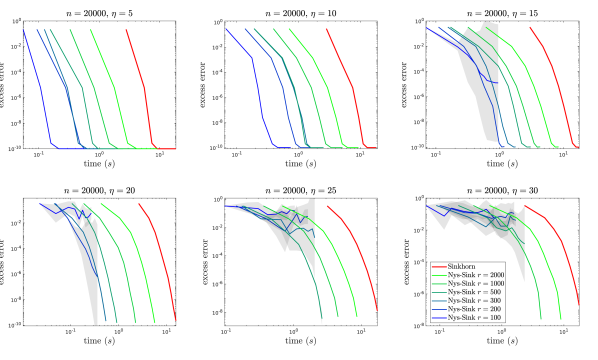
Figure 1: Time-accuracy tradeoff for Nys-Sink and Sinkhorn, for a range of regularization parameters $\eta$ (each corresponding to a different Sinkhorn distance $W_{\eta}$) and approximation ranks $r$. Each experiment has been repeated $50$ times; the variance is indicated by the shaded area around the curves. Note that curves in the plot start at different points corresponding to the time required for initialization.

Fig. 1 plots the time-accuracy tradeoff for Nys-Sink, compared to the standard Sinkhorn algorithm. This experiment is run on random point clouds of size $n\approx 20000$, which corresponds to cost matrices of dimension approximately $20000\times 20000$. Fig. 1 shows that Nys-Sink is consistently orders of magnitude faster to obtain the same accuracy.

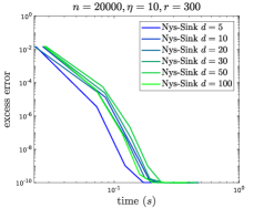
Figure 2: Left: one-dimensional curve embedded in $\mathbb{R}^{d}$, for $d=3$. For $d\geqslant 4$, the curve we use in dimension $d$ is obtained from the curve we use in the dimension $d-1$ by adding a perpendicular segment of length $1/d^{2}$ to one endpoint. Right: Accuracy of Nys-Sink as a function of running time, for different ambient dimensions. Each experiment uses a fixed approximation rank $r=300$.

Next, we investigate Nys-Sink’s dependence on the intrinsic dimension and ambient dimension of the input. This is done by running Nys-Sink on distributions supported on $1$-dimensional curves embedded in higher dimensions, illustrated in Fig. 2, left. Fig. 2, right, indicates that an approximation rank of $r=300$ is sufficient to achieve an error smaller than $10^{-4}$ for any ambient dimension $5\leqslant d\leqslant 100$. This empirically validates the result in 4, namely that the approximation rank – and consequently the computational complexity of Nys-Sink – is independent of the ambient dimension.

Experiment 1: $n\approx 3\times 10^{5}$	$W_{\eta}$	time (s)
Nys-Sink $(r=2000,T=20)$	0.087 $\pm$ 0.008	0.4 $\pm$ 0.1
Dual-Sink + Annealing $(\alpha=0.95)$	0.087	35.4
Dual-Sink Multiscale + Annealing $(\alpha=0.95)$	0.090	3.4

Experiment 2: $n\approx 3.8\times 10^{6}$	$W_{\eta}$	time (s)
Nys-Sink $(r=2000,T=20)$	0.11 $\pm$ 0.01	6.3 $\pm$ 0.8
Dual-Sink + Annealing $(\alpha=0.95)$	0.10	1168
Dual-Sink Multiscale + Annealing $(\alpha=0.95)$	0.11	103.6

Table 1: Comparison of our proposed algorithm to existing, highly-optimized GPU-based algorithms, on a large-scale computer graphics benchmark dataset.

Finally, we evaluate the performance of our algorithm on a benchmark dataset used in computer graphics: we measure Wasserstein distance between 3D cloud points from “The Stanford 3D Scanning Repository”. In the first experiment, we measure the distance between armadillo ($n=1.7\times 10^{5}$ points) and dragon (at resolution 2, $n=1.0\times 10^{5}$ points), and in the second experiment we measure the distance between armadillo and xyz-dragon which has more points ($n=3.6\times 10^{6}$ points). The point clouds are centered and normalized in the unit cube. The regularization parameter is set to $\eta=15$, reflecting the moderate regularization regime typically used in practice.

We compare our algorithm (Nys-Sink)—run with approximation rank $r=2000$ for $T=20$ iterations on a GPU—against two algorithms implemented in the library GeomLoss. These algorithms are both highly optimized and implemented for GPUs. They are: (a) an algorithm based on an annealing heuristic for $\eta$ (controlled by the parameter $\alpha$, such that at each iteration $\eta_{t}=\alpha\eta_{t-1}$, see Kosowsky and Yuille, 1994b) and (b) a multiresolution algorithm based on coarse-to-fine clustering of the dataset together with the annealing heuristic (Schmitzer, 2019). Table 1 reports the results, which demonstrate that our method is comparable in terms of precision, and has computational time that is orders of magnitude smaller than the competitors. We note the parameters $r$ and $T$ for Nys-Sink are chosen by hand to balance precision and time complexity.

We note that in these experiments, instead of using Algorithm 2 to choose the rank adaptively, we simply run experiments with a small fixed choice of $r$. As our experiments demonstrate, Nys-Sink achieves good empirical performance even when the rank $r$ is smaller than our theoretical analysis requires. Investigating this empirical success further is an interesting topic for future study.

Appendix A Pseudocode for subroutines

A.1 Pseudocode for Sinkhorn algorithm

As mentioned in the main text, we use the following variant of the classical Sinkhorn algorithm for our theoretical results. Note that in this paper, $\tilde{K}$ is not stored explicitly but instead is stored in factored form. This enables the Sinkhorn algorithm to be implemented quickly since all computations using $\tilde{K}$ are matrix-vector multiplications with $\tilde{K}$ and $\tilde{K}^{T}$ (see discussion in 3.1 for details).

1:$\tilde{K}$ (in factored form), $\mathbf{p},\mathbf{q}\in\Delta_{n}$, $\delta>0$

2:Positive diagonal matrices $D_{1},D_{2}\in\mathbb{R}^{n\times n}$, cost $\hat{W}$

3:$\tau\leftarrow\tfrac{\delta}{8}$, $D_{1},D_{2}\leftarrow I_{n\times n}$, $k\leftarrow 0$

4:$\mathbf{p}^{\prime}\leftarrow(1-\tau)\mathbf{p}+\frac{\tau}{n}\mathbf{1}$, $\mathbf{q}^{\prime}\leftarrow(1-\tau)\mathbf{q}+\frac{\tau}{n}\mathbf{1}$ $\triangleright$ Round $\mathbf{p}$ and $\mathbf{q}$

5:while $\|D_{1}\tilde{K}D_{2}\mathbf{1}-\mathbf{p}^{\prime}\|_{1}+\|(D_{1}\tilde{K}D_{2})^{\top}\mathbf{1}-\mathbf{q}^{\prime}\|_{1}\leqslant\tfrac{\delta}{2}$ do

6:     $k\leftarrow k+1$

7:     if $k$ odd then

8:         $(D_{1})_{ii}\leftarrow\mathbf{p}^{\prime}_{i}/(\tilde{K}D_{2}\mathbf{1})_{i}$ for $i=1,\dots,n$. $\triangleright$ Renormalize rows

9:     else

10:         $(D_{2})_{jj}\leftarrow\mathbf{q}^{\prime}_{j}/((D_{1}\tilde{K})^{\top}\mathbf{1})_{j}$ for $j=1,\dots,n$. $\triangleright$ Renormalize columns

11:     end if

12:end while

13:$\hat{W}\leftarrow\sum_{i=1}^{n}\log(D_{1})_{ii}(D_{1}\tilde{K}D_{2})\mathbf{1})_{i}+\sum_{j=1}^{n}\log(D_{2})_{jj}((D_{1}\tilde{K}D_{2})^{\top}\mathbf{1})_{j}$

14:return $D_{1}$, $D_{2}$, $\hat{W}$

Algorithm 3 Sinkhorn

Lemma A.

Let $\tilde{C}:=-\eta^{-1}\log\tilde{K}$ and let $\tilde{P}:=D_{1}\tilde{K}D_{2}$, where $D_{1}$ and $D_{2}$ are the scaling matrices output by Sinkhorn. Then the output $\hat{W}$ of Sinkhorn satisfies $\hat{W}=V_{\tilde{C}}(\tilde{P})$. Moreover, computing $\hat{W}$ takes time $O(\textsc{T}_{\textsc{mult}}+n)$, where $\textsc{T}_{\textsc{mult}}$ is the time required to take matrix-vector products with $\tilde{K}$ and $\tilde{K}^{\top}$.

Proof.

Then

$$\langle\tilde{C},\tilde{P}\rangle-\eta^{-1}H(\tilde{P}) =\langle\tilde{C},\tilde{P}\rangle+\eta^{-1}\sum_{i,j=1}^{n}\tilde{P}_{ij}\log\tilde{P}_{ij}$$

$$=\langle\tilde{C},\tilde{P}\rangle+\eta^{-1}\sum_{i,j=1}^{n}\tilde{P}_{ij}(\log(D_{1})_{ii}+\log(D_{2})_{jj}-\eta\tilde{C}_{ij})$$

$$=\sum_{i,j=1}^{n}\tilde{P}_{ij}\log(D_{1})_{ii}+\sum_{i,j=1}^{n}\tilde{P}_{ij}\log(D_{2})_{jj}$$

$$=\sum_{i=1}^{n}\log(D_{1})_{ii}(\tilde{P}\mathbf{1})_{i}+\sum_{j=1}^{n}\log(D_{2})_{jj}(\tilde{P}^{\top}\mathbf{1})_{j}=\hat{W}\,.$$

Moreover, the matrices $\log(D_{1})$ and $\log(D_{2})$ can each be formed in $O(n)$ time, so computing $\hat{W}$ takes time $O(\textsc{T}_{\textsc{mult}}+n)$, as claimed. ∎

A.2 Pseudocode for rounding algorithm

For completeness, here we briefly recall the rounding algorithm Round from (Altschuler et al., 2017) and prove a slight variant of their Lemma 7 that we need for our purposes.

It will be convenient to develop a little notation. For a vector $x\in\mathbb{R}^{n}$, $\mathbb{D}(x)$ denotes the $n\times n$ diagonal matrix with diagonal entries $[\mathbb{D}(x)]_{ii}=x_{i}$. For a matrix $A$, $r(A):=A\mathbf{1}$ and $c(A):=A^{T}\mathbf{1}$ denote the row and column marginals of $A$, respectively. We further denote $r_{i}(A)=[r(A)]_{i}$ and similarly $c_{j}(A):=[c(A)]_{j}$.

1:$F\in\mathbb{R}^{n\times n}$ and $\mathbf{p},\mathbf{q}\in\Delta_{n}$

2:$G\in\mathcal{M}(\mathbf{p},\mathbf{q})$

3:$X\leftarrow\mathbb{D}(x)$, where $x_{i}:=\tfrac{\mathbf{p}_{i}}{r_{i}(F)}\wedge 1$

4:$F^{\prime}\leftarrow XF$

5:$Y\leftarrow\mathbb{D}(y)$, where $y_{j}:=\tfrac{\mathbf{q}_{j}}{c_{j}(F^{\prime})}\wedge 1$

6:$F^{\prime\prime}\leftarrow F^{\prime}Y$

7:$\text{err}_{r}\leftarrow\mathbf{p}-r(F^{\prime\prime})$, $\text{err}_{c}\leftarrow\mathbf{q}-c(F^{\prime\prime})$

8:Output $G\leftarrow F^{\prime\prime}+\text{err}_{r}\text{err}_{c}^{T}/\|\text{err}_{r}\|_{1}$

Algorithm 4 Round (from Algorithm 2 in (Altschuler et al., 2017))

Lemma B.

If $\mathbf{p},\mathbf{q}\in\Delta_{n}$ and $F\in\mathbb{R}_{\geqslant 0}^{n\times n}$, then $\textsc{Round}(F,\mathbf{p},\mathbf{q})$ outputs a matrix $G\in\mathcal{M}(\mathbf{p},\mathbf{q})$ of the form $G=D_{1}FD_{2}+uv^{\top}$ for positive diagonal matrices $D_{1}$ and $D_{2}$ satisfying

$$\|G-F\|_{1}\leqslant\left[\|F\mathbf{1}-\mathbf{p}\|_{1}+\|F^{T}\mathbf{1}-\mathbf{q}\|_{1}\right].$$

Moreover, the algorithm only uses $O(1)$ matrix-vector products with $F$ and $O(n)$ additional processing time.

Proof.

The runtime claim is clear. Next, let $\Delta:=\|F\|_{1}-\|F^{\prime\prime}\|_{1}=\sum_{i=1}^{n}(r_{i}(F)-\mathbf{p}_{i})_{+}+\sum_{j=1}^{n}(c_{j}(F^{\prime})-\mathbf{q}_{j})_{+}$ denote the amount of mass removed from $F$ to create $F^{\prime\prime}$. Observe that $\sum_{i=1}^{n}(r_{i}(F)-\mathbf{p}_{i})_{+}=\operatorname{\frac{1}{2}}\|r(F)-\mathbf{p}\|_{1}$. Since $F^{\prime}\leqslant F$ entrywise, we also have $\sum_{j=1}^{n}(c_{j}(F^{\prime})-\mathbf{q}_{j})_{+}\leqslant\sum_{j=1}^{n}(c_{j}(F)-\mathbf{q}_{j})_{+}=\operatorname{\frac{1}{2}}\|c(F)-\mathbf{q}\|_{1}$. Thus $\Delta\leqslant\operatorname{\frac{1}{2}}(\|r(F)-\mathbf{p}\|_{1}+\|c(F)-q\|_{1})$. The proof is complete since $\|F-G\|_{1}\leqslant\|F-F^{\prime\prime}\|_{1}+\|F^{\prime\prime}-G\|_{1}=2\Delta$. ∎

Appendix B Omitted proofs

B.1 Stability inequalities for Sinkhorn distances

Lemma C.

Let $C,\tilde{C}\in\mathbb{R}^{n\times n}$. If $P\in\Delta_{n\times n}$, then

$$|V_{C}(P)-V_{\tilde{C}}(P)|\leqslant\|C-\tilde{C}\|_{\infty}\,.$$

Proof.

By Hölder’s inequality, $|V_{C}(P)-V_{\tilde{C}}(P)|=|\langle C-\tilde{C},P\rangle|\leqslant\|C-\tilde{C}\|_{\infty}\|P\|_{1}=\|C-\tilde{C}\|_{\infty}$. ∎

Lemma D.

Let $P,Q\in\Delta_{n\times n}$. If $\|P-Q\|_{1}\leqslant\delta\leqslant 1$, then

$$|H(P)-H(Q)|\leqslant\delta\log\frac{2n}{\delta}\,.$$

Proof.

By Ho and Yeung (2010, Theorem 6), $|H(P)-H(Q)|\leqslant\frac{\delta}{2}\log(n^{2}-1)+h\big{(}\frac{\delta}{2}\big{)}$, where $h$ is the binary entropy function. If $\delta\leqslant 1$, then $h(\frac{\delta}{2})\leqslant\delta\log\frac{2}{\delta}$, which yields the claim. ∎

Lemma E.

Let $M\in\mathbb{R}^{n\times n}$, $\eta>0$, and $P,Q\in\Delta_{n\times n}$. If $\|P-Q\|_{1}\leqslant\delta\leqslant 1$, then

$$\left\lvert V_{M}(P)-V_{M}(Q)\right\rvert\leqslant\delta\|M\|_{\infty}+\eta^{-1}\delta\log\frac{2n}{\delta}\,.$$

Proof.

By definition of $V_{M}(\cdot)$ and the triangle inequality, $|V_{M}(P)-V_{M}(Q)|\leqslant|\sum_{ij}(P_{ij}-Q_{ij})M_{ij}|+\eta^{-1}|H(P)-H(\tilde{P})|$. By Hölder’s inequality, the former term is upper bounded by $\|P-Q\|_{1}\|M\|_{\infty}\leqslant\delta\|M\|_{\infty}$. By Lemma D, the latter term above is upper bounded by $\eta^{-1}\delta\log\tfrac{2n}{\delta}$. ∎

B.2 Bregman divergence of Sinkhorn distances

The remainder in the first-order Taylor expansion of $V_{C}(\cdot)$ between any two joint distributions is exactly the KL-divergence between them.

Lemma F.

For any $C\in\mathbb{R}^{n\times n}$, $\eta>0$, and $P,Q\in\Delta^{n\times n}$,

$$V_{C}(Q)=V_{C}(P)+\langle\nabla V_{C}(P),(Q-P)\rangle+\eta^{-1}\mathsf{KL}(Q\|P).$$

Proof.

Observing that $\nabla V_{C}(P)$ has $ij$th entry $C_{ij}+\eta^{-1}(1+\log P_{ij})$, we expand the right hand side as $[\langle C,P\rangle+\eta^{-1}\sum_{ij}P_{ij}\log P_{ij}]+[\langle C,Q-P\rangle+\eta^{-1}\sum_{ij}(Q_{ij}-P_{ij})\log P_{ij}\rangle]+[\eta^{-1}\sum_{ij}Q_{ij}\log\frac{Q_{ij}}{P_{ij}}]=\langle C,Q\rangle+\eta^{-1}\sum_{ij}Q_{ij}\log Q_{ij}=V_{C}(Q)$. ∎

B.3 Hausdorff distance between transport polytopes

Lemma G.

Let $d_{H}$ denote the Hausdorff distance with respect to $\|\cdot\|_{1}$. If $\mathbf{p},\tilde{\mathbf{p}},\mathbf{q},\tilde{\mathbf{q}}\in\Delta_{n}$, then

$$d_{H}(\mathcal{M}(\mathbf{p},\mathbf{q}),\mathcal{M}(\tilde{\mathbf{p}},\tilde{\mathbf{q}}))\leqslant\|\mathbf{p}-\tilde{\mathbf{p}}\|_{1}+\|\mathbf{q}-\tilde{\mathbf{q}}\|_{1}\,.$$

Proof.

Follows immediately from Lemma B. ∎

Lemma H.

Fix a norm $\|\cdot\|$ on $\mathcal{X}$. If $f:\mathcal{X}\to\mathbb{R}$ satisfies $|f(x)-f(y)|\leqslant\omega(\|x-y\|)$ for $\omega$ an increasing, upper semicontinuous function, then for any two sets $A,B\subseteq\mathcal{X}$,

$$\left\lvert\inf_{x\in A}f(x)-\inf_{x\in B}f(x)\right\rvert\leqslant\omega(d_{H}(A,B))\,,$$

where $d_{H}(A,B)$ is the Hausdorff distance between $A$ and $B$ with respect to $\|\cdot\|$.

Proof.

$$\inf_{x\in A}f(x)-\inf_{x\in B}f(x) \leqslant\adjustlimits{\sup}_{y\in B}{\inf}_{x\in A}f(x)-f(y)$$

$$\leqslant\adjustlimits{\sup}_{y\in B}{\inf}_{x\in A}\omega(\|x-y\|)$$

$$\leqslant\omega(\adjustlimits{\sup}_{y\in B}{\inf}_{x\in A}\|x-y\|)$$

$$\leqslant\omega(d_{H}(A,B))\,.$$

Interchanging the role of $A$ and $B$ yields the claim. ∎

B.4 Miscellaneous helpful lemmas

Lemma I.

Let $X\subset\mathbb{R}^{d}$ be convex, and let $f:X\to\mathbb{R}$ be $1$-strongly-convex with respect to some norm $\|\cdot\|$. If $x_{a}^{*}=\operatorname*{argmin}_{x\in\mathcal{X}}\langle a,x\rangle+f(x)$ and $x^{*}_{b}=\operatorname*{argmin}_{x\in\mathcal{X}}\langle b,x\rangle+f(x)$, then

$$\|x_{a}^{*}-x^{*}_{b}\|\leqslant\|a-b\|_{*}\,,$$

where $\|\cdot\|_{*}$ denotes the dual norm to $\|\cdot\|$.

Proof.

This amounts to the well known fact (see, e.g., Hiriart-Urruty and Lemaréchal, 2001, Theorem 4.2.1) that the Legendre transform of a strongly convex function has Lipschitz gradients. We assume without loss of generality that $f=+\infty$ outside of $\mathcal{X}$, so that $f$ can be extended to a function on all of $\mathbb{R}^{d}$ and thus we can take the minima to be unconstrained. The fact that $f(y)+\langle y,a\rangle\geqslant f(x^{*}_{a})+\langle x^{*}_{a},a\rangle$ for all $y$ implies that $-a\in\partial f(x^{*}_{a})$, and likewise $-b\in\partial f(x^{*}_{b})$. Thus by definition of strong convexity, we have

$$f(x^{*}_{a}) \geqslant f(x^{*}_{b})+\langle-b,x^{*}_{a}-x^{*}_{b}\rangle+\operatorname{\frac{1}{2}}\|x^{*}_{a}-x^{*}_{b}\|^{2},$$

$$f(x^{*}_{b}) \geqslant f(x^{*}_{a})+\langle-a,x^{*}_{b}-x^{*}_{a}\rangle+\operatorname{\frac{1}{2}}\|x^{*}_{b}-x^{*}_{a}\|^{2},$$

Adding these inequalities yields

$$\langle b-a,x^{*}_{a}-x^{*}_{b}\rangle\geqslant\|x^{*}_{a}-x^{*}_{b}\|^{2}\,,$$

which implies the claim via the definition of the dual norm. ∎

Lemma J.

For any matrix $A\in\mathbb{R}^{n\times n}$,

$$\|A\|_{\infty}\leqslant\|A\|_{\mathrm{op}}\leqslant n\|A\|_{\infty}$$

Proof.

By duality between the operator norm and the nuclear norm, $\|A\|_{\infty}=\max_{i,j\in[n]}|e_{i}^{T}Ae_{j}|\leqslant\max_{i,j\in[n]}\|A\|_{\mathrm{op}}\|e_{i}e_{j}^{T}\|_{*}=\|A\|_{\mathrm{op}}$. This establishes the first inequality.

Next, for any $v\in\mathbb{R}^{n}$ with unit norm $\|v\|_{2}=1$, note that $\|Av\|^{2}_{2}=\sum_{i=1}^{n}\left(\sum_{j=1}^{n}A_{ij}v_{j}\right)^{2}\leqslant\sum_{i=1}^{n}n\|A\|^{2}_{\infty}\sum_{j=1}^{n}v_{j}^{2}=n^{2}\|A\|^{2}_{\infty}$, proving the second inequality. ∎

Lemma K.

For any $a,b>0$,

$$|\log a-\log b|\leqslant\frac{|a-b|}{\min\{a,b\}}\,.$$

Proof.

Without loss of generality, assume $a\geqslant b$. Then $\log a-\log b=\log\tfrac{a}{b}\leqslant\tfrac{a}{b}-1=\tfrac{a-b}{\min\{a,b\}}\,,$ as claimed. ∎

Lemma L.

Let $\{x_{1},\dots,x_{n}\}\subset\mathbb{R}^{d}$ lie in an Euclidean ball of radius $R$, and let $\eta>0$. Denote by $K\in\mathbb{R}^{n\times n}$ the matrix with entries $K_{ij}:=e^{-\eta\|x_{i}-x_{j}\|_{2}^{2}}$. If a matrix $\widetilde{K}\in\mathbb{R}^{n\times n}$ satisfies $\|K-\widetilde{K}\|_{\infty}\leqslant\frac{\varepsilon^{\prime}}{2}e^{-4\eta R^{2}}$ for some $\varepsilon^{\prime}\in(0,1)$, then

$$\|\log K-\log\widetilde{K}\|_{\infty}\leqslant\varepsilon^{\prime}\,.$$

Proof.

Since $\|x_{i}\|_{2}\leqslant R$ for all $i\in[n]$, the matrix $K$ satisfies $K_{ij}=e^{-\eta\|x_{i}-x_{j}\|_{2}^{2}}\geqslant e^{-4\eta R^{2}}$ for all $i,j\in[n]$. Hence $\widetilde{K}_{ij}\geqslant\tfrac{\varepsilon^{\prime}}{2}e^{-4\eta R^{2}}$ for all $i,j\in[n]$ and thus by Lemma K,

$$|\log K_{ij}-\log\widetilde{K}_{ij}|\leqslant\frac{|K_{ij}-\widetilde{K}_{ij}|}{\min\{\widetilde{K}_{ij},K_{ij}\}}\leqslant\varepsilon^{\prime}\,.$$

∎

Lemma M.

Let $n\in\mathbb{N}$, $\varepsilon\in(0,1)$, $\|C\|_{\infty}\geqslant 1$, and $\eta\in[1,n]$. Then for any $\delta\leqslant\tfrac{\eta\varepsilon}{50(\|C\|_{\infty}\eta+\log\tfrac{n}{\eta\varepsilon})}$, the bound $\delta(2\|C\|_{\infty}+3\eta^{-1})+2\eta^{-1}\delta\log\tfrac{2n}{\delta}\leqslant\tfrac{\varepsilon}{2}$ holds.

Proof.

We write

$$\delta(2\|C\|_{\infty}+3\eta^{-1})+2\eta^{-1}\delta\log\tfrac{2n}{\delta}=\delta(2\|C\|_{\infty}+3\eta^{-1})+2\eta^{-1}\delta\log\tfrac{2n}{\eta\varepsilon}+2\eta^{-1}\delta\log\tfrac{\eta\varepsilon}{\delta}$$

and bound the three terms separately. First, the assumptions imply that $\eta\varepsilon\leqslant n$ and $2\|C\|_{\infty}+3\eta^{-1}\leqslant 5\|C\|_{\infty}$. We therefore have

$$\delta(2\|C\|_{\infty}+3\eta^{-1})\leqslant\frac{5\|C\|_{\infty}\eta\varepsilon}{50(\|C\|_{\infty}\eta+\log\tfrac{n}{\eta\varepsilon})}\leqslant\frac{1}{10}\varepsilon\,.$$

Since $\|C\|_{\infty}\eta\geqslant 1$, we likewise obtain

$$2\eta^{-1}\delta\log\frac{2n}{\eta\varepsilon}\leqslant\frac{2\varepsilon\log\frac{2n}{\eta\varepsilon}}{50(1+\log\frac{n}{\eta\varepsilon})}=\frac{2(\log 2+\log\frac{n}{\eta\varepsilon})}{50(1+\log\frac{n}{\eta\varepsilon})}\varepsilon\leqslant\frac{1}{25}\varepsilon\,.$$

Finally, the fact that $\tfrac{\eta^{-1}\delta}{\varepsilon}\leqslant\tfrac{1}{50}$ and $x\log\frac{1}{x}\leqslant\tfrac{1}{10}$ for $x\leqslant\tfrac{1}{50}$ yields

$$2\eta^{-1}\delta\log\tfrac{\eta\varepsilon}{\delta}=2\left(\tfrac{\eta^{-1}\delta}{\varepsilon}\log\tfrac{\varepsilon}{\eta^{-1}\delta}\right)\varepsilon\leqslant\frac{1}{5}\varepsilon\,.$$

∎

B.5 Supplemental results for Section 3

B.5.1 Full proof of Theorem 3

Define $\phi_{\alpha}(x):=(2\eta)^{\sum_{j=1}^{d}\alpha_{j}/2}\prod_{j=1}^{d}[(\alpha_{j}!)^{-1/2}x_{j}^{\alpha_{j}}e^{-\eta x_{j}^{2}}]$, for $x\in\mathbb{R}^{d}$ and $\alpha\in(\mathbb{N}\cup\{0\})^{d}$, and define $\psi_{T}(x):=(\phi_{\alpha}(x))_{\alpha_{1}+\dots+\alpha_{d}\leqslant T}$. Note that $\psi_{T}:\mathbb{R}^{d}\to\mathbb{R}^{M}$, with $M=\binom{d+T}{T}$. By Cotter et al. (2011, equation 11), we have

$$\sup_{x,x^{\prime}\in B_{R}^{d}}|k_{\eta}(x,x^{\prime})-\psi_{T}(x)^{\top}\psi_{T}(x^{\prime})|\leqslant\frac{(2\eta R^{2})^{T+1}}{(T+1)!}=:\varepsilon(T).$$

Now denote by $\Psi_{T}\in\mathbb{R}^{M\times n}$ the matrix $\Psi_{T}:=(\psi_{T}(x_{1}),\dots,\psi_{T}(x_{n}))$. By Lemma J, we have

$$\|K-\Psi_{T}^{\top}\Psi_{T}\|_{\text{op}}\leqslant n\sup_{i,j}|k_{\eta}(x_{i},x_{j})-\psi_{T}(x_{i})^{\top}\psi_{T}(x_{j})|\leqslant n\varepsilon(T).$$

By the Eckart-Young-Mirsky Theorem, we have

$$\lambda_{M+1}=\inf_{\bar{K}_{T}\in\mathbb{R}^{n\times n},\,\text{rank}(\bar{K}_{T})\leqslant M}\|K-\bar{K}_{T}\|_{\text{op}}.$$

Therefore by combining the above two displays, we conclude that

$$\lambda_{M+1}\leqslant\|K-\Psi_{T}^{\top}\Psi_{T}\|_{\text{op}}\leqslant n\varepsilon(T).$$

Point 1.

We recall that for any $d,q\in\mathbb{N}$, the inequality $\binom{d+q}{q}\leqslant e^{d}(1+q/d)^{d}$ holds. Therefore, given $t\geqslant(2e)^{d}$, choosing $T=\lfloor dt^{1/d}/(2e)\rfloor$ yields $\binom{T+d}{d}\leqslant e^{d}(1+T/d)^{d}\leqslant t$. We therefore have $\lambda_{t+1}\leqslant n\varepsilon(T)$ for this choice of $T$. Now, by Stirling’s approximation of $(T+1)!$, we have that $\varepsilon(T)\leqslant e^{-(T+1)\log{T+1\over 2e\eta R^{2}}}$. If $T\geqslant 2e\eta R^{2}$, then $(T+1)\log{T+1\over 2e\eta R^{2}}\geqslant\tfrac{dt^{1/d}}{2e}\log\tfrac{dt^{1/d}}{4e^{2}\eta R^{2}}$, which yields the desired bound. On the other hand, when $T<2e\eta R^{2}$, we use the trivial bound $\lambda_{t}(K)\leqslant\operatorname{Tr}(K)\leqslant n$. The claim follows.

Point 2.

We have that $\lambda_{M_{T}+1}(K)\leqslant n\varepsilon(T)$, for $M_{T}=\binom{d+T}{T}$ and $T\in\mathbb{N}$. Since the eigenvalues are in decreasing order we have that $\lambda_{M_{T+1}+1}\leqslant\lambda_{t}(K)\leqslant\lambda_{M_{T}+1}(K)$ for $M_{T}+1\leqslant t\leqslant M_{T+1}+1$. Since $x/(x+\tau)$ is increasing in $x$, for $x\geqslant 0$, we have

$$\sum_{t=1}^{n}\frac{\lambda_{j}(K)}{\lambda_{j}(K)+n\tau}\leqslant\sum_{T=0}^{\infty}(M_{T+1}-M_{T})\frac{\lambda_{M_{T}+1}(K)}{\lambda_{M_{T}+1}(K)+n\tau}\leqslant\sum_{T=0}^{\infty}(M_{T+1}-M_{T})\frac{\varepsilon(T)}{\varepsilon(T)+\tau}.$$

Let $T_{\tau}$ be such that $\varepsilon(T_{\tau})\leqslant\tau$. We can then bound $\varepsilon(T)/(\varepsilon(T)+\tau)$ above by $1$ for $T\leqslant T_{\tau}-1$ and by $\varepsilon(T)/\tau$ for $T\geqslant T_{\tau}$, obtaining

$$\sum_{T=0}^{\infty}(M_{T+1}-M_{T})\frac{\varepsilon(T)}{\varepsilon(T)+\tau} \leqslant\sum_{T=0}^{T_{\tau}-1}(M_{T+1}-M_{T})~{}+~{}\sum_{T=T_{\tau}}^{\infty}(M_{T+1}-M_{T})\frac{\varepsilon(T)}{\tau}$$

$$=M_{T_{\tau}}+\frac{1}{\tau}\sum_{T=T_{\tau}}^{\infty}(M_{T+1}-M_{T})\varepsilon(T).$$

In particular, we can choose $T_{\tau}=d+2e^{2}\eta R^{2}+\log(1/\tau)$. Since $\log\frac{T_{\tau}}{2e\eta R^{2}}>1$, for any $T\geqslant T_{\tau}$, then $\varepsilon(T)\leqslant e^{-T\log\frac{T}{2e\eta R^{2}}}\leqslant e^{-T}$. Moreover since $M_{T+1}-M_{T}=dM_{T}/(T+1)$, and $M_{T}\leqslant e^{d}(1+T/d)^{d}$, we have

$$\sum_{T=T_{\tau}}^{\infty}(M_{T+1}-M_{T})\varepsilon(T) \leqslant\frac{d}{T_{\tau}}\sum_{T=T_{\tau}}^{\infty}M_{T}e^{-T}\leqslant\frac{de^{d}}{T_{\tau}}\sum_{T=T_{\tau}}^{\infty}\left(1+{T\over d}\right)^{d}e^{-T}$$

$$\leqslant\frac{de^{d}}{T_{\tau}}\int_{T_{\tau}}^{\infty}\left(1+{x\over d}\right)^{d}e^{-x}dx.$$

Finally, by changing variables, $x=u+T_{\tau}$ and $u=(d+T_{\tau})z$,

$$\int_{T_{\tau}}^{\infty}\left(1+{x\over d}\right)^{d}e^{-x}dx =\int_{0}^{\infty}\left(1+{T_{\tau}\over d}+{u\over d}\right)^{d}e^{-u-T_{\tau}}du$$

$$=\left(1+{T_{\tau}\over d}\right)^{d}e^{-T_{\tau}}\int_{0}^{\infty}\left(1+{u\over d+T_{\tau}}\right)^{d}e^{-u}du$$

$$=\left(1+{T_{\tau}\over d}\right)^{d}e^{-T_{\tau}}(d+T_{\tau})\int_{0}^{\infty}\left(1+z\right)^{d}e^{-(d+T_{\tau})z}dz$$

$$=d^{-d}e^{d}\Gamma(d+1,d+T_{\tau}),$$

where for the last equality we used the characterization of the incomplete gamma function $\Gamma(a,z)=z^{-a}e^{-z}\int_{0}^{\infty}(1+t)^{a-1}e^{-zt}dt$ (see Eq. 8.6.5 of Olver et al., 2010). To complete the proof note that by P we have $\Gamma(a,z)\leqslant z/(z-a)z^{a-1}e^{-z}$, for any $z>a>0$. Since $\log(1/\tau)\geqslant 0$ for $\tau\in(0,1]$, we have $(d+T_{\tau})/(T_{\tau}-1)\leqslant 2$ and $(de^{-T_{\tau}})/(\tau T_{\tau})\leqslant 1$, so

$$d_{\textrm{eff}}(\tau) \leqslant M_{T_{\tau}}+\frac{de^{d}}{\tau T_{\tau}}d^{-d}e^{d}\Gamma(d+1,d+T_{\tau})$$

$$\leqslant e^{d}(1+T_{\tau}/d)^{d}\left(1+\frac{de^{-T_{\tau}}}{\tau T_{\tau}}\frac{d+T_{\tau}}{T_{\tau}-1}\right)$$

$$\leqslant 3e^{d}\left(2+\frac{2e^{2}}{d}\eta R^{2}+\frac{1}{d}\log\frac{1}{\tau}\right)^{d}.$$

∎

B.5.2 Full proof of Theorem 4

The proof of Points 2 and 3 here is completely analogous to the proof of Points 1 and 2, respectively, in Theorem 3.

Point 2.

Let $\bar{X}=\{\bar{x}_{1},\dots,\bar{x}_{p}\}\subset\Omega$ be a minimal $\varepsilon$ net of $\Omega$. Since $\Omega$ is a smooth manifold of dimension $k$, then there exists $C_{0}>0$ for which $p\leqslant C_{0}\varepsilon^{-k}$. Now let $\bar{K}\in\mathbb{R}^{p\times p}$ be given by $\bar{K}_{i,j}=k_{\eta}(\bar{x}_{i},\bar{x}_{j})$ and define $\Phi(x)=\bar{K}^{-1/2}v(x)$, with $v(x)=(k_{\eta}(x,\bar{x}_{1}),\dots,k_{\eta}(x,\bar{x}_{p}))$. Then when $f(x^{\prime}):=k_{\eta}(x^{\prime},x)$, then $\widehat{f}_{\bar{X}}=\Phi(x^{\prime})^{\top}\Phi(x)$. By applying Point 1 to $f(x)=k_{\eta}(x^{\prime},x)$, we have

$$|k_{\eta}(x^{\prime},x)-\Phi(x^{\prime})\Phi(x)|\leqslant e^{-c\varepsilon^{-2/5}},\qquad\forall x,x^{\prime}\in\Omega.$$

If we let $B\in\mathbb{R}^{p\times n}=(\Phi(x_{1}),\dots\Phi(x_{n}))$, then

$$\|K-B^{\top}B\|_{\text{op}}\leqslant n\max_{ij}|k_{\eta}(x^{\prime},x)-\Phi(x^{\prime})\Phi(x)|\leqslant ne^{-c\varepsilon^{-2/5}}.$$

Since $B$ is of rank $p$, the the Eckart-Young-Mirsky Theorem again implies $\lambda_{p+1}(K)\leqslant ne^{-c\varepsilon^{-2/5}}$. We conclude by recalling that $\varepsilon\leqslant(p/C_{0})^{-1/k}$.

Point 3.

Let $M_{\tau}$ be such that $\lambda_{M_{\tau}+1}\leqslant n\tau$. By Point 2, this holds if we take $M_{\tau}=(c_{0}\log\tfrac{1}{\tau})^{5k/2}$ for a sufficiently large constant $c$. By definition of $d_{\textrm{eff}}(\tau)$ and the fact that $x/(x+\lambda)\leqslant\min(1,x/\lambda)$ for any $x\geqslant 0,\lambda>0$, we have

$$d_{\textrm{eff}}(\tau) =\sum_{j=1}^{n}\frac{\lambda_{j}(K)}{\lambda_{j}(K)+n\tau}=\sum_{j=1}^{M_{\tau}+1}\frac{\lambda_{j}(K)}{\lambda_{j}(K)+n\tau}+\sum_{j=M_{\tau}+2}^{n}\frac{\lambda_{j}(K)}{\lambda_{j}(K)+n\tau}$$

$$\leqslant M_{\tau}+1+\frac{1}{\tau}\sum_{j=M_{\tau}+2}^{n}\frac{\lambda_{j}(K)}{n}\leqslant(c_{0}\log\tfrac{1}{\tau})^{5k/2}+1+\frac{1}{\tau}\sum_{j=M_{\tau}+1}^{\infty}e^{-cj^{\frac{2}{5k}}}$$

Denoting $\beta:=\tfrac{2}{5k}$ for shorthand, we can upper bound the sum as follows:

$$\sum_{j=M_{\tau}+1}^{\infty}e^{-cj^{\tfrac{2}{5k}}} \leqslant\int_{M_{\tau}}^{\infty}e^{-cx^{\beta}}dx$$

$$=\frac{1}{\beta c^{1/\beta}}\int_{0}^{\infty}u^{\frac{1-\beta}{\beta}}\mathds{1}(u\geqslant cM_{\tau}^{\beta})e^{-u}du$$

$$\leqslant\frac{1}{\beta c^{1/\beta}}\left(\int_{0}^{\infty}u^{2(\tfrac{1-\beta}{\beta})}e^{-u}du\right)^{1/2}\left(\int_{cM_{\tau}^{\beta}}^{\infty}e^{-u}du\right)^{1/2}$$

$$=c_{k}e^{-\operatorname{\frac{1}{2}}cM_{\tau}^{\beta}}\leqslant c_{k}\tau,$$

where above the second step was by the change of variables $u:=cx^{\beta}$, the third step was by Cauchy-Schwartz with respect to the inner product $\langle f,g\rangle:=\int_{0}^{\infty}f(u)g(u)e^{-u}du$, and the final line was for some constant $c_{k}$ only depending on $k$, whenever $c_{0}$ is taken to be at least $\tfrac{2}{c}$. This proves the claim. ∎

B.5.3 Additional bounds

Lemma N.

Let $A:B\to U$, be a smooth map, with $B\subseteq\mathbb{R}^{d}$, $U\subseteq\mathbb{R}^{m}$, $d,m\in\mathbb{N}$, such that there exists $Q>0$, for which

$$\|D^{\alpha}A\|_{L^{\infty}(B)}\leqslant Q^{|\alpha|},\quad\forall\alpha\in\mathbb{N}^{d},$$

then, for $\nu\in\mathbb{N}_{0}^{d}$, $p\geqslant 1$,

$$\|D^{\nu}(f\circ A)\|_{L^{p}(B)}\leqslant(2|\nu|mQ)^{|\nu|}\max_{|\lambda|\leqslant|\nu|}\|(D^{\lambda}f)\circ A\|_{L^{p}(B)}.$$

Proof.

First we study $D^{\nu}(f\circ A)$. Let $n:=|\nu|$ and $A=(a_{1},\dots,a_{m})$ with $a_{j}:\mathbb{R}^{d}\to\mathbb{R}$. By the multivariate Faa di Bruno formula (Constantine and Savits, 1996), we have that

$$D^{\nu}(f\circ A)=\nu!\sum_{1\leqslant|\lambda|\leqslant n}(D^{\lambda}f)\circ A\sum_{\tiny\begin{pmatrix}k_{1}\dots,k_{n}\\ l_{1},\dots,l_{n}\end{pmatrix}\in p(\lambda,\nu)}~{}~{}\prod_{j=1}^{n}\prod_{i=1}^{m}\frac{[D^{l_{j}}a_{i}]^{[k_{j}]_{i}}}{[k_{j}]_{i}!l_{j}!},$$

where the set $p(\lambda,\nu)$ is defined in Constantine and Savits (1996, Eq. 2.4), with $l_{1},\dots,l_{n}\in\mathbb{N}_{0}^{d}$, $k_{1},\dots,k_{n}\in\mathbb{N}_{0}^{m}$ and satisfying $\sum_{j=1}^{n}|k_{j}|l_{j}=\nu$. Now by assumption $\|D^{l_{j}}a_{i}\|\leqslant Q^{|l_{j}|}$ for $1\leqslant i\leqslant m$. Then

$$\left\|\prod_{j=1}^{n}\prod_{i=1}^{m}\frac{[D^{l_{j}}a_{i}]^{[k_{j}]_{i}}}{[k_{j}]_{i}!l_{j}!}\right\|_{L^{\infty}(B)}\leqslant Q^{\sum_{j=1}^{n}|l_{j}||k_{j}|}\prod_{j=1}^{n}\frac{1}{k_{j}!l_{j}!^{|k_{j}|}}.$$

Now note that by the properties of $l_{j},k_{j}$, we have that $|\nu|=|\sum_{j}|k_{j}|l_{j}|=\sum_{j}|k_{j}||l_{j}|,$ then

$$\|D^{\nu}(f\circ A)\|_{L^{p}(B)}\leqslant Q^{|\nu|}\max_{|\lambda|\leqslant|\nu|}\|(D^{\lambda}f)\circ A\|_{L^{p}(B)}~{}~{}\times~{}~{}\nu!\sum_{1\leqslant|\lambda|\leqslant n}\sum_{\tiny\begin{matrix}k_{1}\dots,k_{n}\\ l_{1},\dots,l_{n}\end{matrix}\in p(\lambda,\nu)}~{}\prod_{j=1}^{n}\frac{1}{k_{j}!l_{j}!^{|k_{j}|}}.$$

To conclude, denote by $S^{n}_{k}$ the Stirling numbers of the second kind. By Constantine and Savits (1996, Corollary 2.9) and Rennie and Dobson (1969) we have

$$\nu!\sum_{1\leqslant|\lambda|\leqslant n}\sum_{\tiny\begin{matrix}k_{1}\dots,k_{n}\\ l_{1},\dots,l_{n}\end{matrix}\in p(\lambda,\nu)}~{}\prod_{j=1}^{n}\frac{1}{k_{j}!l_{j}!^{|k_{j}|}}=\sum_{i=1}^{n}m^{k}S^{n}_{k}\leqslant m^{n}\sum_{i=1}^{n}\binom{n}{k}k^{n-k}\leqslant m^{n}(2n)^{n}.$$

∎

Lemma O.

Let $\Psi_{j}:U_{j}\to B^{k}_{r_{j}}$ such that there exists $Q>0$ for which $\|D^{\alpha}\Psi_{j}^{-1}\|_{L^{\infty}(B^{k}_{r_{j}})}\leqslant Q^{|\alpha|}$ for $\alpha\in\mathbb{N}^{k}$. Then for any $q\geqslant k$, we have

$$\|f\circ\Psi_{j}^{-1}\|_{W^{q}_{2}(B^{k}_{r_{j}})}\leqslant C_{d,k,R,r_{j}}q^{k}(2qdQ)^{q}\|f\|_{W^{q+(d+1)/2}_{2}(B^{d}_{R})}.$$

Proof.

First note that $\|\cdot\|_{L^{\infty}(B^{d}_{R})}\leqslant C_{d,R}\|\cdot\|_{W^{(d+1)/2}_{2}(B^{d}_{R})}$ (Adams and Fournier, 2003) for a constant $C_{d,R}$ depending only on $d$ and $R$. Therefore

$$\|(D^{\alpha}f)\circ\Psi_{j}^{-1}\|_{L^{2}(B^{k}_{r_{j}})} \leqslant\textrm{vol}(B^{k}_{r_{j}})^{1/2}\|(D^{\alpha}f)\circ\Psi_{j}^{-1}\|_{L^{\infty}(B^{k}_{r_{j}})}$$

$$=\textrm{vol}(B^{k}_{r_{j}})^{1/2}\|D^{\alpha}f\|_{L^{\infty}(U_{j})}\leqslant\textrm{vol}(B^{k}_{r_{j}})^{1/2}\|D^{\alpha}f\|_{L^{\infty}(B^{d}_{R})}$$

$$\leqslant C_{d,R}\textrm{vol}(B^{k}_{r_{j}})^{1/2}\|D^{\alpha}f\|_{W^{(d+1)/2}_{2}(B^{d}_{R})}.$$

Moreover note that $\|D^{\alpha}f\|_{W^{(d+1)/2}_{2}(B^{d}_{R})}\leqslant\|f\|_{W^{|\alpha|+(d+1)/2}_{2}(B^{d}_{R})}$. By N we have that

$$\|D^{\alpha}(f\circ\Psi_{j}^{-1})\|_{L^{2}(B^{k}_{r_{j}})}\leqslant(2|\alpha|dQ)^{|\alpha|}\max_{|\lambda|\leqslant|\alpha|}\|(D^{\lambda}f)\circ\Psi_{j}^{-1}\|_{L^{2}(B^{k}_{r_{j}})}.$$

By definition of Sobolev space $W^{q}_{2}(B^{k}_{r_{j}})$, we have

$$\|f\circ\Psi_{j}^{-1}\|_{W^{q}_{2}(B^{k}_{r_{j}})} \leqslant\sum_{|\alpha|\leqslant q}\|D^{\alpha}(f\circ\Psi_{j}^{-1})\|_{L^{2}(B^{k}_{r_{j}})}$$

$$\leqslant\sum_{|\alpha|\leqslant q}(2|\alpha|dQ)^{|\alpha|}\max_{|\lambda|\leqslant|\alpha|}\|(D^{\lambda}f)\circ\Psi_{j}^{-1}\|_{L^{2}(B^{k}_{r_{j}})}$$

$$\leqslant C_{q}\max_{|\lambda|\leqslant q}\|(D^{\lambda}f)\circ\Psi_{j}^{-1}\|^{2}_{L^{2}(B^{k}_{r_{j}})},$$

where $C_{q}:=\sum_{|\alpha|\leqslant q}(2|\alpha|dQ)^{|\alpha|}$. Then,

$$\|f\circ\Psi_{j}^{-1}\|^{2}_{W^{q}_{2}(B^{k}_{r_{j}})}\leqslant C_{q}C_{d,R}\textrm{vol}(B^{k}_{r_{j}})^{1/2}\|f\|_{W^{q+(d+1)/2}_{2}(B^{d}_{R})}.$$

The final result is obtained via the bound $C_{q}\leqslant(2qdQ)^{q}\binom{k+q}{k}\leqslant(2ek)^{k}(2qdQ)^{q}q^{k}$ for $q\geqslant k$. ∎

Lemma P (Bounds for the incomplete gamma function).

Denote by $\Gamma(a,x)$ the function defined as

$$\Gamma(a,x)=\int_{x}^{\infty}z^{a-1}e^{-z}dz,$$

for $a\in\mathbb{R}$ and $x>0$. When $x\geqslant(a-1)_{+}~{}\wedge~{}x>0$, the following holds

$$\Gamma(a,x)\leqslant\frac{x}{x-(a-1)_{+}}x^{a-1}e^{-x},$$

In particular $\Gamma(a,x)\leqslant 2x^{a-1}e^{-x},$ for $x\geqslant 2(a-1)_{+}~{}\wedge~{}x>0$.

Proof.

Assume $x>0$. When $a\leqslant 1$, the function $z^{a-1}e^{-z}$ is decreasing and in particular $z^{a-1}e^{-z}\leqslant x^{a-1}e^{-z}$ for $z\geqslant x$, so when $z\geqslant x$ we have

$$\Gamma(a,x)=\int_{x}^{\infty}z^{a-1}e^{-z}dz\leqslant x^{a-1}\int_{x}^{\infty}e^{-z}dz=x^{a-1}e^{-x}.$$

When $a>1$, for any $\tau\in(0,1)$, we have

$$\Gamma(a,x) =\int_{x}^{\infty}z^{a-1}e^{-z}dz=\int_{x}^{\infty}(z^{a-1}e^{-\tau z})(e^{-(1-\tau)z})dz$$

$$\leqslant\sup_{z\geqslant x}(z^{a-1}e^{-\tau z})~{}\int_{x}^{\infty}e^{-(1-\tau)z}dz=\frac{e^{-(1-\tau)x}}{1-\tau}\sup_{z\geqslant x}(z^{a-1}e^{-\tau z}).$$

Now note that the maximum of $z^{a-1}e^{-\tau z}$ is reached when $z=(a-1)/\tau$. When $x\geqslant a-1$, we can set $\tau=(a-1)/x$, so the maximum of $z^{a-1}e^{-\tau z}$ is exactly in $z=x$. In that case $\sup_{z\geqslant x}(z^{a-1}e^{-\tau z})=x^{a-1}e^{-\tau x}$ and

$$\Gamma(a,x)\leqslant\frac{x}{x-(a-1)}x^{a-1}e^{-x}.$$

The final result is obtained by gathering the cases $a\leqslant 1$ and $a>0$ in the same expression. ∎

Corollary A.

Let $a\in\mathbb{R}$, $A,q_{1},q_{2},b>0$. When $q_{2}A^{b}\geqslant 2\left(\frac{a+1}{b}-1\right)_{+}$, the following holds

$$\int_{A}^{\infty}q_{1}x^{a}e^{-q_{2}x^{b}}dx\leqslant\frac{2q_{1}}{bq_{2}}A^{a+1-1/b}e^{-q_{2}A^{b}}.$$

Proof.

By the change of variable $x=(u/q_{2})^{1/b}$ we have

$$\int_{A}^{\infty}q_{1}x^{a}e^{-q_{2}x^{b}}dx =\frac{q_{1}q_{2}^{-\frac{a+1}{b}}}{b}\int_{q_{2}A^{b}}^{\infty}u^{\frac{a+1}{b}-1}e^{-u}du$$

$$=\frac{q_{1}q_{2}^{-\frac{a+1}{b}}}{b}\Gamma\left(\frac{a+1}{b},q_{2}A^{b}\right)$$

$$\leqslant\frac{2q_{1}}{bq_{2}}A^{a+1-1/b}e^{-q_{2}A^{b}},$$

where for the last step we used P. ∎

Appendix C Lipschitz properties of the Sinkhorn projection

We give a simple construction illustrating that the Sinkhorn projection operator is not Lipschitz in the standard sense. This stands in contrast with Proposition 2, which illustrates that this projection is Lipschitz on the logarithmic scale.

This non-Lipschitz result holds even for the following simple rescaling of the $2\times 2$ Birkhoff polyope:

$$\mathcal{M}:=\left\{P\in\mathbb{R}_{\geqslant 0}^{2\times 2}\;:\;P1=P^{T}1=\begin{bmatrix}\operatorname{\frac{1}{2}}\\ \operatorname{\frac{1}{2}}\end{bmatrix}\right\}.$$

Proposition 4.

The Sinkhorn projection operator onto $\mathcal{M}$ is not Lipschitz for any norm on $\mathbb{R}^{2\times 2}$.

Proof.

By the equivalence of finite-dimensional norms, it suffices to prove this for $\|\cdot\|_{1}$, for which we will show

$$\sup_{K,K^{\prime}\in\Delta_{2,2}\cap\mathbb{R}_{>0}^{2\times 2}}\frac{\left\|\Pi_{\mathcal{M}}^{\mathcal{S}}(K)-\Pi_{\mathcal{M}}^{\mathcal{S}}(K^{\prime})\right\|_{1}}{\|K-K^{\prime}\|_{1}}=\infty.$$ (9)

The restriction to strictly positive matrices $\mathbb{R}_{>0}^{2\times 2}$ (rather than non-negative matrices) is to ensure that there is no issue of existence of Sinkhorn projections (see, e.g., Linial et al., 1998, Section 2).

For $\varepsilon,\delta\in(0,1)$, define the matrix

$$K_{\varepsilon,\delta}:=\begin{bmatrix}1-\varepsilon&\varepsilon\\ 1-\delta&\delta\end{bmatrix}$$

and let $P_{\varepsilon,\delta}:=\Pi_{\mathcal{M}}^{\mathcal{S}}(K_{\varepsilon,\delta})$ denote the Sinkhorn projection of $K_{\varepsilon,\delta}$ onto $\mathcal{M}$. The polytope $\mathcal{M}$ is parameterizable by a single scalar as follows:

$$\mathcal{M}=\left\{M_{a}\;:\;a\in[0,1/2]\right\}\,,\quad\quad M_{a}:=\begin{bmatrix}a&\operatorname{\frac{1}{2}}-a\\ \operatorname{\frac{1}{2}}-a&a\end{bmatrix}\,.$$

By definition, $P_{\varepsilon,\delta}$ is the unique matrix in $\mathcal{M}$ of the form $D_{1}K_{\varepsilon,\delta}D_{2}$ for positive diagonal matrices $D_{1}$ and $D_{2}$. Taking

$$D_{1}=\begin{bmatrix}\sqrt{\tfrac{\delta}{\varepsilon}}&0\\ 0&\sqrt{\tfrac{1-\varepsilon}{1-\delta}}\end{bmatrix}\,,\quad\quad D_{2}=\frac{1}{\beta_{\varepsilon,\delta}}\begin{bmatrix}\sqrt{\tfrac{\varepsilon}{1-\varepsilon}}&0\\ 0&\sqrt{\tfrac{1-\delta}{\delta}}\end{bmatrix}$$

for $\beta_{\varepsilon,\delta}=2(\sqrt{\delta(1-\varepsilon)}+\sqrt{\varepsilon(1-\delta)})$, we verify $D_{1}K_{\varepsilon,\delta}D_{2}=M_{a_{\varepsilon,\delta}}$, where $a_{\varepsilon,\delta}:=\frac{\sqrt{\delta(1-\varepsilon)}}{\beta_{\varepsilon,\delta}}$. Therefore $P_{\varepsilon,\delta}=M_{a_{\varepsilon,\delta}}$ for $\varepsilon,\delta\in(0,1)$.

Now parameterize $\varepsilon:=c\delta$ for some fixed constant $c\in(0,\infty)$ and consider taking $\delta\to 0^{+}$. Then $a_{c\delta,\delta}=\frac{\sqrt{1-c\delta}}{2\left[\sqrt{c(1-\delta)}+\sqrt{1-c\delta}\right]}$, which for fixed $c$ becomes arbitrarily close to

$$g(c):=\frac{1}{2(\sqrt{c}+1)}$$

as $\delta$ approaches $0$. Thus $\|P_{c\delta,\delta}-M_{g(c)}\|_{1}=o_{\delta}(1)$ and similarly $\|P_{\delta/c,\delta}-M_{g(1/c)}\|_{1}=o_{\delta}(1)$. We therefore conclude that for any constant $c\in(0,\infty)\setminus\{1\}$, although

$$\|K_{c\delta,\delta}-K_{\delta/c,\delta}\|_{1}=2\delta\left\lvert c-1/c\right\rvert=o_{\delta}(1),$$

vanishes as $\delta\to 0^{+}$, the quantity

$$\left\|\Pi_{\mathcal{M}}^{\mathcal{S}}(K_{c\delta,\delta})-\Pi_{\mathcal{M}}^{\mathcal{S}}(K_{\delta/c,\delta})\right\|_{1} =\left\|P_{c\delta,c}-P_{\delta/c,c}\right\|_{1}$$

$$=\left\|M_{g(c)}-M_{g(1/c)}\right\|_{1}+o_{\delta}(1)$$

$$=4\left\lvert g(c)-g(1/c)\right\rvert+o_{\delta}(1)$$

does not vanish. Therefore combining the above two displays and taking, e.g., $c=2$ proves (9). ∎

References

- Adams and Fournier (2003) R. A. Adams and J. J. Fournier. Sobolev spaces, volume 140. Elsevier, 2003.
- Alaoui and Mahoney (2015) A. Alaoui and M. W. Mahoney. Fast randomized kernel ridge regression with statistical guarantees. In Adv. NIPS, pages 775–783, 2015.
- Allen-Zhu et al. (2017) Z. Allen-Zhu, Y. Li, R. Oliveira, and A. Wigderson. Much faster algorithms for matrix scaling. In FOCS, pages 890–901. 2017.
- Altschuler et al. (2017) J. Altschuler, J. Weed, and P. Rigollet. Near-linear time approximation algorithms for optimal transport via Sinkhorn iteration. In Adv. NIPS, pages 1961–1971, 2017.
- Altschuler et al. (2018) J. Altschuler, F. Bach, A. Rudi, and J. Weed. Approximating the quadratic transportation metric in near-linear time. arXiv preprint arXiv:1810.10046, 2018.
- Arjovsky et al. (2017) M. Arjovsky, S. Chintala, and L. Bottou. Wasserstein GAN. arXiv preprint arXiv:1701.07875, 2017.
- Bach (2013) F. Bach. Sharp analysis of low-rank kernel matrix approximations. In Conference on Learning Theory, pages 185–209, 2013.
- Belkin (2018) M. Belkin. Approximation beats concentration? An approximation view on inference with smooth radial kernels. arXiv preprint arXiv:1801.03437, 2018.
- Blanchet et al. (2018) J. Blanchet, A. Jambulapati, C. Kent, and A. Sidford. Towards optimal running times for optimal transport. arXiv preprint arXiv:1810.07717, 2018.
- Bousquet et al. (2017) O. Bousquet, S. Gelly, I. Tolstikhin, C.-J. Simon-Gabriel, and B. Schoelkopf. From optimal transport to generative modeling: the VEGAN cookbook. arXiv preprint arXiv:1705.07642, 2017.
- Bubeck (2015) S. Bubeck. Convex optimization: Algorithms and complexity. Foundations and Trends in Machine Learning, 8(3-4):231–357, 2015.
- Cohen et al. (2017) M. B. Cohen, A. Madry, D. Tsipras, and A. Vladu. Matrix scaling and balancing via box constrained Newton’s method and interior point methods. In FOCS, pages 902–913. 2017.
- Constantine and Savits (1996) G. Constantine and T. Savits. A multivariate Faa di Bruno formula with applications. Transactions of the American Mathematical Society, 348(2):503–520, 1996.
- Cotter et al. (2011) A. Cotter, J. Keshet, and N. Srebro. Explicit approximations of the gaussian kernel. arXiv preprint arXiv:1109.4603, 2011.
- Courty et al. (2014) N. Courty, R. Flamary, and D. Tuia. Domain adaptation with regularized optimal transport. In ECML PKDD, pages 274–289, 2014.
- Courty et al. (2017) N. Courty, R. Flamary, D. Tuia, and A. Rakotomamonjy. Optimal transport for domain adaptation. IEEE Trans. Pattern Anal. Mach. Intell., 39(9):1853–1865, 2017.
- Cuturi (2013) M. Cuturi. Sinkhorn distances: Lightspeed computation of optimal transport. In Adv. NIPS, pages 2292–2300, 2013.
- Dvurechensky et al. (2018) P. Dvurechensky, A. Gasnikov, and A. Kroshnin. Computational optimal transport: Complexity by accelerated gradient descent is better than by Sinkhorn’s algorithm. arXiv preprint arXiv:1802.04367, 2018.
- Fine and Scheinberg (2001) S. Fine and K. Scheinberg. Efficient SVM training using low-rank kernel representations. Journal of Machine Learning Research, 2:243–264, 2001.
- Forrow et al. (2018) A. Forrow, J.-C. Hütter, M. Nitzan, P. Rigollet, G. Schiebinger, and J. Weed. Statistical optimal transport via factored couplings. arXiv preprint arXiv:1806.07348, 2018.
- Franklin and Lorenz (1989) J. Franklin and J. Lorenz. On the scaling of multidimensional matrices. Linear Algebra Appl., 114/115:717–735, 1989.
- Friedman et al. (2001) J. Friedman, T. Hastie, and R. Tibshirani. The elements of statistical learning, volume 1. Springer series in statistics New York, NY, USA:, 2001.
- Fuselier and Wright (2012) E. Fuselier and G. B. Wright. Scattered data interpolation on embedded submanifolds with restricted positive definite kernels: Sobolev error estimates. SIAM Journal on Numerical Analysis, 50(3):1753–1776, 2012.
- Genevay et al. (2016) A. Genevay, M. Cuturi, G. Peyré, and F. Bach. Stochastic optimization for large-scale optimal transport. In Adv. NIPS, pages 3440–3448. 2016.
- Genevay et al. (2018) A. Genevay, G. Peyré, and M. Cuturi. Learning generative models with Sinkhorn divergences. In AISTATS, pages 1608–1617, 2018.
- Gittens (2011) A. Gittens. The spectral norm error of the naive Nyström extension. Arxiv preprint arXiv:1110.5305, 2011.
- Hangelbroek et al. (2010) T. Hangelbroek, F. J. Narcowich, and J. D. Ward. Kernel approximation on manifolds I: bounding the Lebesgue constant. SIAM Journal on Mathematical Analysis, 42(4):1732–1760, 2010.
- Hiriart-Urruty and Lemaréchal (2001) J.-B. Hiriart-Urruty and C. Lemaréchal. Fundamentals of convex analysis. Grundlehren Text Editions. Springer-Verlag, Berlin, 2001.
- Ho and Yeung (2010) S.-W. Ho and R. W. Yeung. The interplay between entropy and variational distance. IEEE Trans. Inform. Theory, 56(12):5906–5929, 2010.
- Kalantari et al. (2008) B. Kalantari, I. Lari, F. Ricca, and B. Simeone. On the complexity of general matrix scaling and entropy minimization via the RAS algorithm. Math. Program., 112(2, Ser. A):371–401, 2008.
- Kolouri et al. (2017) S. Kolouri, S. R. Park, M. Thorpe, D. Slepcev, and G. K. Rohde. Optimal mass transport: Signal processing and machine-learning applications. IEEE Signal Process. Mag., 34(4):43–59, 2017.
- Kosowsky and Yuille (1994a) J. Kosowsky and A. L. Yuille. The invisible hand algorithm: Solving the assignment problem with statistical physics. Neural Networks, 7(3):477–490, 1994a.
- Kosowsky and Yuille (1994b) J. Kosowsky and A. L. Yuille. The invisible hand algorithm: Solving the assignment problem with statistical physics. Neural networks, 7(3):477–490, 1994b.
- Li et al. (2013) P. Li, Q. Wang, and L. Zhang. A novel earth mover’s distance methodology for image matching with Gaussian mixture models. In ICCV, pages 1689–1696, 2013.
- Linial et al. (1998) N. Linial, A. Samorodnitsky, and A. Wigderson. A deterministic strongly polynomial algorithm for matrix scaling and approximate permanents. In STOC, pages 644–652. ACM, 1998.
- Mahoney and Drineas (2009) M. W. Mahoney and P. Drineas. CUR matrix decompositions for improved data analysis. PNAS, 106(3):697–702, 2009.
- Montavon et al. (2016) G. Montavon, K. Müller, and M. Cuturi. Wasserstein training of restricted Boltzmann machines. In Adv. NIPS, pages 3711–3719, 2016.
- Musco and Musco (2017) C. Musco and C. Musco. Recursive sampling for the Nystrom method. In Adv. NIPS, pages 3833–3845, 2017.
- Olver et al. (2010) F. W. Olver, D. W. Lozier, R. F. Boisvert, and C. W. Clark. NIST handbook of mathematical functions. Cambridge University Press, 2010.
- Peyré and Cuturi (2017) G. Peyré and M. Cuturi. Computational optimal transport. Technical report, 2017.
- Quanrud (2019) K. Quanrud. Approximating optimal transport with linear programs. In SOSA, 2019. To appear.
- Rennie and Dobson (1969) B. C. Rennie and A. J. Dobson. On Stirling numbers of the second kind. Journal of Combinatorial Theory, 7(2):116–121, 1969.
- Rieger and Zwicknagl (2010) C. Rieger and B. Zwicknagl. Sampling inequalities for infinitely smooth functions, with applications to interpolation and machine learning. Advances in Computational Mathematics, 32(1):103, 2010.
- Rigollet and Weed (2018) P. Rigollet and J. Weed. Entropic optimal transport is maximum-likelihood deconvolution. Comptes Rendus Mathématique, 2018. To appear.
- Rubner et al. (2000) Y. Rubner, C. Tomasi, and L. J. Guibas. The earth mover’s distance as a metric for image retrieval. International journal of computer vision, 40(2):99–121, 2000.
- Rudi et al. (2018) A. Rudi, D. Calandriello, L. Carratino, and L. Rosasco. On fast leverage score sampling and optimal learning. arXiv preprint arXiv:1810.13258, 2018.
- Schiebinger et al. (2019) G. Schiebinger, J. Shu, M. Tabaka, B. Cleary, V. Subramanian, A. Solomon, S. Liu, S. Lin, P. Berube, L. Lee, et al. Reconstruction of developmental landscapes by optimal-transport analysis of single-cell gene expression sheds light on cellular reprogramming. Cell, 2019. To appear.
- Schmitzer (2019) B. Schmitzer. Stabilized sparse scaling algorithms for entropy regularized transport problems. SIAM Journal on Scientific Computing, 41(3):A1443–A1481, 2019.
- Shawe-Taylor and Cristianini (2004) J. Shawe-Taylor and N. Cristianini. Kernel Methods for Pattern Analysis. Camb. U. P., 2004.
- Simon (1979) B. Simon. A remark on Dobrushin’s uniqueness theorem. Comm. Math. Phys., 68(2):183–185, 1979.
- Sinkhorn (1967) R. Sinkhorn. Diagonal equivalence to matrices with prescribed row and column sums. The American Mathematical Monthly, 74(4):402–405, 1967.
- Smola and Schölkopf (2000) A. J. Smola and B. Schölkopf. Sparse greedy matrix approximation for machine learning. In Proc. ICML, 2000.
- Solomon et al. (2015) J. Solomon, F. de Goes, G. Peyré, M. Cuturi, A. Butscher, A. Nguyen, T. Du, and L. Guibas. Convolutional Wasserstein distances: Efficient optimal transportation on geometric domains. ACM Trans. Graph., 34(4):66:1–66:11, July 2015.
- Tenetov et al. (2018) E. Tenetov, G. Wolansky, and R. Kimmel. Fast Entropic Regularized Optimal Transport Using Semidiscrete Cost Approximation. SIAM J. Sci. Comput., 40(5):A3400–A3422, 2018.
- Villani (2008) C. Villani. Optimal transport: old and new, volume 338. Springer Science & Business Media, 2008.
- Wendland (2004) H. Wendland. Scattered data approximation, volume 17. Cambridge university press, 2004.
- Williams and Seeger (2001) C. Williams and M. Seeger. Using the Nyström method to speed up kernel machines. In Adv. NIPS, 2001.
- Wilson (1969) A. G. Wilson. The use of entropy maximising models, in the theory of trip distribution, mode split and route split. Journal of Transport Economics and Policy, pages 108–126, 1969.
- Zhang (2005) T. Zhang. Learning bounds for kernel regression using effective data dimensionality. Neural Computation, 17(9):2077–2098, 2005.