Detections and Constraints on White Dwarf Variability from Time-Series GALEX Observations

Abstract

We search for photometric variability in more than 23,000 known and candidate white dwarfs, the largest ultraviolet survey compiled for a single study of white dwarfs. We use gPhoton, a publicly available calibration/reduction pipeline, to generate time-series photometry of white dwarfs observed by GALEX. By implementing a system of weighted metrics, we select sources with variability due to pulsations and eclipses. Although GALEX observations have short baselines ($\leq 30$ min), we identify intrinsic variability in sources as faint as Gaia $G=20$ mag. With our ranking algorithm, we identify 49 new variable white dwarfs (WDs) in archival GALEX observations. We detect 41 new pulsators: 37 have hydrogen-dominated atmospheres (DAVs), including one possible massive DAV, and four are helium-dominated pulsators (DBVs). We also detect eight new eclipsing systems; five are new discoveries, and three were previously known spectroscopic binaries. We perform synthetic injections of the light curve of WD 1145+017, a system with known transiting debris, to test our ability to recover similar systems. We find that the $3\sigma$ maximum occurrence rate of WD 1145+017-like transiting objects is $\leq 0.5\%$.

1 Introduction

More than 97% of all stars in our Galaxy, including our Sun, will end their lives as white dwarfs (WDs). Not only do WDs offer a lens into degenerate matter physics not replicable on Earth, but they also describe end-stage stellar evolution and planetary systems. By measuring photometric variation in these stars, we can test theoretical models of internal WD structure and energy transfer.

One way WDs vary is through pulsations. By characterizing the pulsation modes of white dwarf stars, fundamental parameters of the star, including mass, core composition, and internal structure can be determined (Fontaine & Brassard, 2008; Althaus et al., 2010). This technique, known as asteroseismlology, can supplement spectroscopic WD observations, which can constrain $T_{\rm{eff}}$ and $\log g$. Asteroseismology allows us to trace the interior effects of stellar evolution, from the main sequence to the white dwarf stage (Catalán et al., 2008; Córsico, 2017).

WD pulsators are grouped by their spectral classification. The majority have hydrogen-dominated atmospheres, known as DAV or ZZ Ceti stars, with temperatures ranging from 10,500–12,500 K (Gianninas et al., 2011). Those with helium-dominated atmospheres, DBVs, pulsate at 22,000–29,000 K (Nitta et al., 2009). Each type occupies a distinct parameter space in the $\log g-T_{\rm{eff}}$ diagram (Tremblay et al., 2015). Within both of these classes, pulsations are driven by partial ionization of the dominant atmospheric element (Winget & Kepler, 2008). The brightness variations are generated by global, non-radial gravity ($g$-mode) pulsations that have characteristic timescales typically ranging from $100-1400$ seconds (Koester & Chanmugam, 1990; Hermes et al., 2017).

Besides pulsations, WDs also often exhibit variability due to eclipses. We expect roughly 29$\pm$8% of WDs to currently have a binary companion (Toonen et al., 2017). There are more than 100 WD+WD binaries known with periods less than a day, although fewer than 10 of those are eclipsing sources (Brown et al., 2017). There are also more than 70 eclipsing WD-main sequence binaries that have evolved through a common-envelope phase (Parsons et al., 2015).

Finally, it is possible that transiting planets and/or planetary debris can cause variability in a WD light curve. Disintegrating asteroids/planetesimals have been observed around WD 1145+017 (Vanderburg et al., 2015). Time-series photometry shows distinct periodicities with broad peaks in the power spectrum, possibly indicating trails of debris following the larger orbiting bodies, which causes deep (up to $>$50%) transits in the optical. Roughly 1% of DA WDs have been observed to have an infrared excess from debris disks, indicating the potential for similar detections around sources similar to WD 1145+017 (Farihi, 2016). WD surveys for transiting planets have been conducted with WASP (Faedi et al., 2011), Pan-STARRS1 (Fulton et al., 2014), and K2 (van Sluijs & Van Eylen, 2018). While these surveys yielded no new detections, they placed various upper limits on the occurrence rate for planetary bodies around WDs.

Characterization of WD variability requires high-cadence photometry with a long baseline. To meet these needs, most WD variability surveys have been conducted in the optical regime (e.g., Mukadam et al., 2004). However, since most WDs have blackbodies that peak in the ultraviolet (UV), it is more promising to search for variability at these wavelengths. Space-based photometry allows for UV observations, though these studies often use much shorter observational baselines. Time-tagged light curves from the GALEX space telescope, which observes in two UV bands, was first used for the detection of WD pulsations by Tucker et al. (2018).

In this paper we present variability analysis of 23,676 WDs from archival GALEX photometry. Section §2 outlines the source selection criteria for our survey. We develop a ranking method, described in Section §3, to identify variability. We report the detection of known variables in Section §4, new pulsators in Section §5, and eclipsing binaries in Section §6. Section §7 describes the injection and recovery of asteroids/planetesimals, as well as upper limits on their occurrence. Finally, we summarize our results in Section §8.

2 GALEX Observations & Survey Selection

Photometric observations for WDs in our survey were taken with the GALEX space telescope (Morrissey et al., 2005; Martin et al., 2005). GALEX observed $\sim 77\%~{}\rm$ of the sky in two ultraviolet bands: the near-ultraviolet (NUV, 1771–2831 Å) and far-ultraviolet (FUV, 1344–1786 Å). GALEX observations were taken during the night side of each orbit, known as an ‘eclipse’, with each observation lasting up to 30 minutes. Most of our WD sources have been observed by GALEX multiple times. We henceforth refer to a single exposure lasting up to 30 minutes as an observation.

2.1 gPhoton

We implement the publicly available GALEX photometry calibration pipeline gPhoton (Million et al., 2016, version 1.28.2) to check GALEX exposure time and produce time-series photometry for each source. We construct light curves with 15-second bins, excluding bins with $<10$ seconds to avoid exposure aliasing. Quality flags output by gPhoton help reduce additional instrumental false positives from entering our data. Four quality flags are excluded: mask edge, detector edge, exposure time, and spacecraft recovery (Million et al., 2016).

To reduce oversaturation for bright sources, GALEX dithers with a 1.5’ spiral (Morrissey et al., 2005; Martin et al., 2005). This can represent itself as a periodicity in flux and counts per second, which must be taken into consideration when identifying variability. For an overview of GALEX/gPhoton instrumental effects and light curve irregularities, see de la Vega & Bianchi (2018).

2.2 Catalog Selection

The WDs in our survey are taken from 4 catalogs:

1. Spectroscopically confirmed and high-probability candidate white dwarfs from the SDSS White Dwarf Catalog (DR8, 10, and 12, Kleinman et al., 2013; Kepler et al., 2015, 2016). We exclude any subdwarfs in this catalog.

2. WDs with probability $P_{\rm{WD}}\geq 0.5$ from VST ATLAS (Gentile Fusillo et al., 2017).

3. Sources from Montreal White Dwarf Database (MWDD, Dufour et al., 2017). This database also provides additional information, including binarity and disks, on WDs in other included catalogs.

4. A cut by color and magnitude in Gaia DR2 (Gaia Collaboration et al., 2018), selecting sources with the criteria:

   • $\displaystyle G+5\log(\frac{\omega}{100})>4(G_{\rm{BP}}-G_{\rm{RP}})$

   • $\displaystyle 1.0+0.015(G_{BP}-G_{RP})<E_{BP/RP}$

   • $\displaystyle 1.3+0.06(G_{BP}-G_{RP})^{2}>E_{BP/RP}$,

     where $G$, $G_{\text{BP}}$, and $G_{\text{RP}}$ are the Gaia passbands, $\omega$ is the parallax in milli-arcseconds, and $E_{\text{BP/RP}}$ is the excess factor measured with respect to the Gaia G band.

   This region is plotted on a color-magnitude diagram in Figure 1. The first criteria divides the WD population in color-magnitude space from the non-WD background plotted in gray. The excess factor criteria is a quality cut for background and contamination issues.

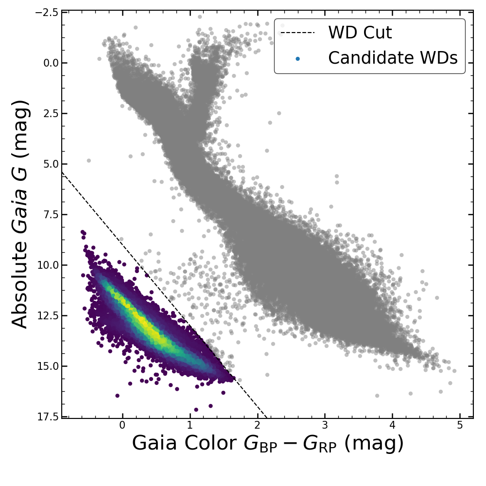
Figure 1: We select WDs from the Gaia DR2 color magnitude diagram using a linear cut described in Section §2.2. WDs included in our survey are colored by density of points.

We cross match coordinates between catalogs to remove duplicates, resulting in 40,856 sources. The catalog is further reduced by selecting sources with GALEX exposure time $>$1000s reported by gPhoton to ensure adequate timescales for detectable variability. After applying these cuts and merging the separate catalogs, the final target list consists of 23,676 WDs, the largest photometric ultraviolet WD survey compiled for a single study (previous largest 320, Tucker et al., 2018).

3 Identifying Variability

To comb through such a large sample, we use a ranking algorithm to prioritize sources more likely to have variability. This system uses four metrics, $c_{LSP}$, $c_{WS}$, $c_{RMS}$, and $c_{EXPT}$. We weight each metric to produce a final rank.

The highest-weighted metric, $c_{LSP}$ with weight $w_{LSP}$, is based on a Lomb-Scargle periodogram (Scargle, 1982; Lomb, 1976, see VanderPlas (2018) for a recent review) of the light curve. The Baluev Method (Baluev, 2008; VanderPlas, 2018) calculates the false-alarm probability of the five highest amplitudes in each periodogram. Peaks are considered to be statistically significant if the false alarm probability is $<5\%$. This threshold is chosen based on the short baselines of GALEX observation, smoothing out high amplitude, narrow peak periodogram features.

We use a Fourier spectrum of the dither position as a function of time output by gPhoton to ensure variability is not due to telescope dither. Peaks overlapping within $8~{}\rm{seconds}$ of the periodicities in the telescope dither are not considered. For most sources, the dither alias falls at approximately $121~{}\rm{seconds}$. If the detected period is larger than the exposure time, the metric is multiplied by $1/8$. This consideration helps to reduce some instrumental artifacts, including the jump and slope variations described by de la Vega & Bianchi (2018). Since each observation for a source is considered separately, there is no aliasing due to observation cadence. The metric $c_{LSP}$ is calculated as

$$c_{LSP}=a_{max}/a_{5\%},$$ (1)

where $a_{max}$ is the amplitude of the highest peak divided by the 5% false alarm probability level $a_{5\%}$. If there are no peaks with false alarm probability less than $5\%$, $c_{LSP}$ is set to zero.

The second metric is based on the variability index defined by Welch & Stetson (1993). For GALEX visits with observations in both NUV and FUV, we promote correlated variability in our weighting scheme. Flux residuals are calculated as

$$\delta_{NUV}=\frac{f_{NUV,i}-\bar{f}_{NUV}}{\sigma_{NUV,i}}$$ (2)

$$\delta_{FUV}=\frac{f_{FUV,i}-\bar{f}_{FUV}}{\sigma_{FUV,i}},$$ (3)

where $f_{NUV,i}$ and $f_{FUV,i}$ is the flux given on a percentage scale:

$$\text{flux}_{\%}=((\text{flux}/\text{median}(\text{flux}))-1.0)\times 100$$ (4)

in $i^{th}$ bin for each band. The metric $c_{WS}$, with weight $w_{WS}$, has the functional form

$$c_{WS}=\frac{1}{n}\sqrt{\frac{n}{n-1}}\sum_{i=1}^{n}\delta_{NUV,i}\delta_{FUV,i}$$ (5)

where $n$ is the number of discrete photometric measurements in the light curve. For random observations, the $i^{th}$ $\delta_{NUV}$ and $\delta_{FUV}$ values will be uncorrelated, averaging out to 0 for the metric (Welch & Stetson, 1993). For light curves without concurrent coverage in both bands we set the $\delta_{other}$, either $\delta_{FUV}$ or $\delta_{NUV}$, to be 1 in the calculation. Since telescope dither is consistent across both bands, this is an additional consideration to reduce false positives. If there is a prominent periodicity (false alarm probability $<25\%$) in the light curve data corresponding to the dither period, we exclude this metric, setting $c_{WS}$ to be zero for the observation. This metric is similar to $c_{RMS}$. We include both in order to promote correlated variability without penalizing single-band observations.

The third-highest-weighted metric, $c_{RMS}$ with weight $w_{RMS}$, considers how the root mean square (RMS) in magnitude ($\sigma_{RMS}$) for a source compares to sources of similar magnitudes. Sources with high amplitudes of variability are expected to have larger scatter in magnitude, as compared to non-varying WDs of a similar magnitude. WDs are binned by NUV and FUV magnitude, with bin sizes 0.1 mag. The $\sigma_{RMS}$ of each source is then compared to the median $\sigma_{RMS}$ of sources in the same magnitude bin. The metric is calculated as $c_{RMS}=RMS/\rm{median}(RMS)$. Many sources have especially high RMS values due to instrumental effects. To reduce this impact on our ranking, we cap the RMS metric at the $95^{\rm{th}}$ percentile, which reduces the false positive rate while still retaining the effectiveness of the metric. This metric is especially helpful in the identification of eclipses, where the decrease in flux is consistent with zero flux.

The final metric is based on exposure time and data-quality flags. Variability is more likely to be detected in sources with longer timescales of observation. Therefore, we use the metric $c_{EXP}$ with weight $w_{EXP}$ to take exposure time into consideration. However, in order to include consideration of removed flagged data, the metric excludes time in flagged bins, computed as $c_{EXP}=t_{\rm{total}}-t_{\rm{flagged}}$.

For each GALEX observation, the rank R is calculated as the sum of the metrics:

$$\begin{split}\mathrm{R}=&w_{LSP}c_{LSP}+w_{WS}c_{WS}+w_{RMS}c_{RMS}+w_{EXP}c_{EXP}\end{split}$$ (6)

Since most of our WDs have multiple distinct GALEX observations, each lasting up to 30 minutes, the final rank for a given WD is the max R value among all observations. This is useful for sifting through sources with long-term or aperiodic variability. The purpose of our ranking system is to quickly identify variability rather than to provide an absolute methodology to compare variable sources. Therefore, weights are adjusted manually using random subsets of our sample to ensure known variable WDs are recovered successfully. The final weights used are given in Table 1. After tuning weights on a smaller scale, we apply the ranking algorithm to the entire sample, producing a list with higher ranked sources more likely to display astrophysical variability.

Even after implementing our ranking system, we do not completely remove false positives from the data. Specifically, there are sources with periodicities due to telescope dither that occasionally have harmonics at higher frequencies. Some FUV observations show a recurring long-term variability that does not correlate with NUV trends. These ‘jump variations’, described in de la Vega & Bianchi (2018), are likely due to instrumental effects with the FUV filter (Morrissey, 2006).

We inspect the top $\sim 10\%$ of ranked sources manually to characterize the type of variability and to remove false positives. After identifying sources with intrinsic variability, we divide our sample into three separate categories: known pulsators, new pulsators, and eclipsing sources. Out of the total 23,676 WDs, we detect 41 new pulsators, 13 known pulsators, 8 new eclipsing WDs, and 1 known eclipsing WD. We plot all 63 variable WDs detected on a GAIA CMD in Figure 2.

Table 1: Weights used in the ranking algorithm described in §3.

Metric	Abbreviation	Weight
Lomb-Scargle Periodogram	$w_{LSP}$	0.5714
Welch-Stetson Index	$w_{WS}$	0.1714
RMS	$w_{RMS}$	0.1429
Exposure (ks)	$w_{EXPT}$	0.1143

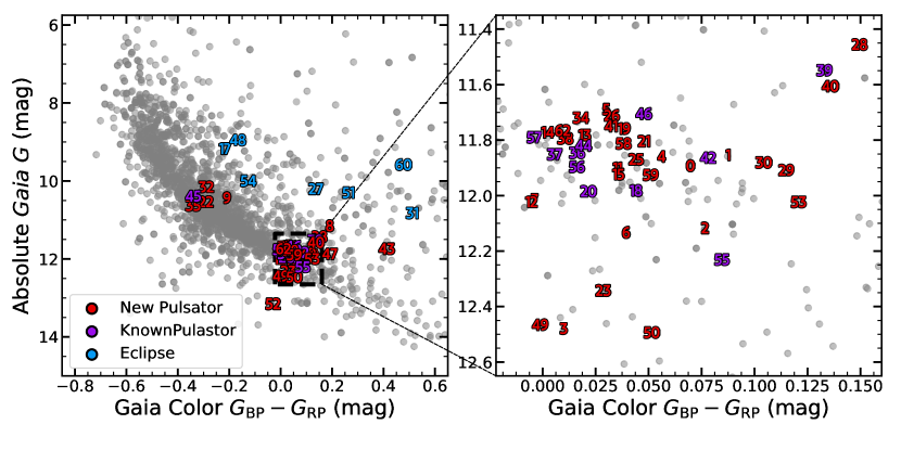
Figure 2: Left: Gaia color-magnitude diagram for the top 3000 ranked sources in our survey. 13 Known pulsators, 41 new pulsators, and 9 eclipsing sources are labeled with their identification number, colored in purple, red, and blue, respectively. We observe two separate populations - DAV stars at $G_{\rm{BP}}-G_{\rm{RP}}\approx 0.1$, M${}_{G}\approx 12$ and DBV pulsators at $G_{\rm{BP}}-G_{\rm{RP}}\approx-0.3$, M${}_{G}\approx 10.5$. Eclipsing sources are overluminous compared to typical WDs at their respective $G_{\rm{BP}}-G_{\rm{RP}}$ colors. Right: Close-in view of instability region for DAV stars.

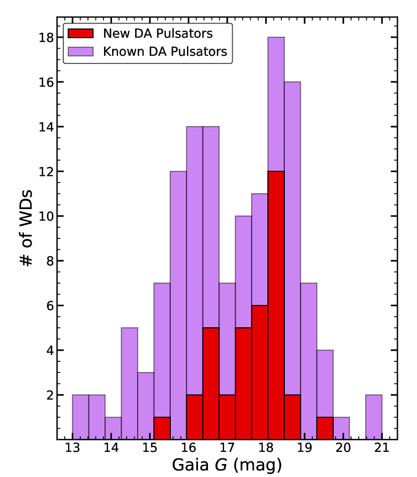
Figure 3: Histogram of apparent magnitudes for new DAV pulsators detected compared to known DAV pulsators in Table 4 of Bognar & Sodor (2016).

4 Known Variables

In addition to the 49 new variables detected, there are 13 known pulsators and one known eclipsing WD in our survey. Identification information for all sources is provided in Table 2, and discovery references are given in Table 3. UV light curves for these sources are plotted in Appendix B.

Table 2: Information on all detected variable WDs. ID numbers are assigned for each variable in this work. Variability period, NUV amplitude, and FUV amplitude are estimated by fitting sinusoids to the light curves. References for known variables are given in Table 3.

Source	ID#	RA	Dec.	$Gaia$ $G$	Classification	Spec. Type	Period	NUV Amp	FUV Amp
		(deg)	(deg)	(mag)			(s)	(%)	(%)
GALEX 2417766833348155164	0	7.44064	14.70402	18.20	New Pulsator	DAV	898$\pm$44	20$\pm$2	52$\pm$7
WD J002959.22$+145812.97$	1	7.49674	14.97027	17.49	New Pulsator	DAV†	948$\pm$47	9$\pm$2	41$\pm$5
WD J003116.51$+474828.39$	2	7.81881	47.80789	18.36	New Pulsator	DAV†	896$\pm$41	18$\pm$3	47$\pm$9
WD J004154.68$-030802.71$	3	10.47781	-3.13409	18.07	New Pulsator	DAV†	865$\pm$55	5$\pm$4	17$\pm$11
WD J010025.6$+421840.22$	4	15.10665	42.31117	16.58	New Pulsator	DAV†	574$\pm$27	8$\pm$1	26$\pm$8
WD J010528.83$+020500.96$	5	16.37012	2.08360	16.73	New Pulsator	DAV†	710$\pm$14	12$\pm$1	34$\pm$3
WD J010539.17$+321846.53$	6	16.41320	32.31292	18.07	New Pulsator	DAV†	407$\pm$10	9$\pm$2	35$\pm$7
KUV 01595$-$1109	7	30.49558	-10.91064	16.89	New Pulsator	DAV	687$\pm$15	14$\pm$1	–
WD J022941.29$-063842.89$	8	37.42204	-6.64525	18.23	New Pulsator	DAV†	754$\pm$16	23$\pm$2	77$\pm$8
WD J025121.71$-125244.85$	9	42.84045	-12.87913	18.23	New Pulsator	DBV†	944$\pm$72	7$\pm$2	11$\pm$3
2MASS J03030835$+$0054438	10	45.78483	0.91225	17.38	Eclipse	DC+M	–	–	–
WD J030648.49$-172332.19$	11	46.70206	-17.39228	16.70	New Pulsator	DAV†	794$\pm$15	17$\pm$1	72$\pm$4
WD J053212.77$-432006.05$	12	83.05323	-43.33501	18.19	New Pulsator	DAV†	451$\pm$15	11$\pm$6	–
WD J080609.2$+111230.83$	13	121.53832	11.20856	18.11	New Pulsator	DAV†	391$\pm$7	8$\pm$6	30$\pm$13
WD J084055.73$+130329.38$	14	130.23221	13.05816	17.22	New Pulsator	DAV†	490$\pm$16	12$\pm$2	34$\pm$5
US 1639	15	131.72060	44.44405	18.19	New Pulsator	DAV	663$\pm$33	16$\pm$3	58$\pm$10
WD J0855$+$0635	16	133.78021	6.59446	17.32	Known Pulsator	DAV	895$\pm$24	19$\pm$2	51$\pm$6
WD J090023.05$+434813.45$	17	135.09604	43.80374	18.38	Eclipse	D?+?	–	–	–
WD J0906$-$0024	18	136.60098	-0.40776	17.87	Known Pulsator	DAV	747$\pm$27	8$\pm$6	14$\pm$18
WD J093250.51$+554315.68$	19	143.21045	55.72102	17.69	New Pulsator	DAV†	510$\pm$17	10$\pm$2	35$\pm$5
WD 0938$+$577	20	145.55490	57.56188	17.49	Known Pulsator	DAV	608$\pm$16	13$\pm$3	–
SDSS J094851.43$+$512448.0	21	147.21425	51.41336	18.57	New Pulsator	DAV	947$\pm$63	14$\pm$10	32$\pm$30
SDSS J102106.69$+$082724.8	22	155.27769	8.45684	17.82	New Pulsator	DBV	471$\pm$11	8$\pm$1	11$\pm$2
SDSS J103642.25$+$211527.9	23	159.17583	21.25773	17.60	New Pulsator	DAV	679$\pm$41	7$\pm$3	23$\pm$5
CBS 130	24	162.68750	33.26500	16.56	New Pulsator	DAV	484$\pm$9	7$\pm$1	30$\pm$4
WD J105046.04$+331546.22$	25	162.69184	33.26284	16.56	New Pulsator	DAV†	484$\pm$9	7$\pm$1	31$\pm$4
SDSS J110505.94$+$583103.0	26	166.27392	58.51735	17.94	New Pulsator	DAV	825$\pm$20	19$\pm$2	81$\pm$7
WD 1104$+$656	27	167.02229	65.36986	18.53	Eclipse	DA+M	–	–	–
WD J115057.43$-055306.58$	28	177.73930	-5.88516	17.44	New Pulsator	DAV†	424$\pm$9	6$\pm$2	18$\pm$10
USNO A2.0 1350-08049341	29	180.78821	45.75564	18.57	New Pulsator	DAV	835$\pm$30	23$\pm$3	–
WD J122155.73$+050621.6$	30	185.48222	5.10600	17.90	New Pulsator	DAV†	1061$\pm$51	19$\pm$2	–
2MASS J12233961$-$0056311	31	185.91504	-0.94200	17.84	Eclipse	DA+M	–	–	–
SDSS J123654.96$+$170918.7	32	189.22881	17.15514	18.17	New Pulsator	DBV	698$\pm$28	9$\pm$1	–
SDSS J124759.03$+$110703.0	33	191.99596	11.11750	19.35	New Pulsator	DAV	672$\pm$46	29$\pm$10	61$\pm$50
WD J124804.04$+282103.46$	34	192.01683	28.35096	18.04	New Pulsator	DAV†	678$\pm$20	13$\pm$4	–
WD J132952.63$+392150.8$	35	202.46928	39.36411	18.01	New Pulsator	DBV†	727$\pm$34	7$\pm$1	–
WD J1355$+$5454	36	208.87929	54.90125	18.67	Known Pulsator	DAV	158$\pm$4	14$\pm$3	15$\pm$7
V* IU Vir	37	210.98747	-15.02017	15.75	Known Pulsator	DAV	586$\pm$8	9$\pm$1	37$\pm$2
WD 1452$+$600	38	223.34756	59.84885	17.18	New Pulsator	DAV	530$\pm$35	5$\pm$2	26$\pm$8
WD J1502$-$0001	39	225.52925	-0.02975	18.72	Known Pulsator	DAV	645$\pm$35	11$\pm$4	80$\pm$13
WD J150626.13$+063845.0$	40	226.60887	6.64583	16.60	New Pulsator	DAV†	635$\pm$8	10$\pm$2	21$\pm$16
WD J150739.31$+074828.54$	41	226.91378	7.80793	18.21	New Pulsator	DAV†	583$\pm$23	14$\pm$2	32$\pm$6
WD J1617$+$4324	42	244.40697	43.41215	18.44	Known Pulsator	DAV	645$\pm$16	9$\pm$9	–
WD J162724.72$+392027.25$	43	246.85299	39.34090	16.23	New Pulsator	DAV†	268$\pm$4	5$\pm$1	18$\pm$2
HS 1625$+$1231	44	247.05510	12.41426	16.27	Known Pulsator	DAV	974$\pm$12	16$\pm$1	55$\pm$3
GD 358	45	251.82582	32.47590	13.59	Known Pulsator	DAV	874$\pm$15	7$\pm$0	8$\pm$0
WD J1700$+$3549	46	255.23032	35.83057	17.36	Known Pulsator	DAV	924$\pm$31	17$\pm$3	46$\pm$26
WD J173351.44$+341012.96$	47	263.46433	34.17027	16.35	New Pulsator	DAV†	793$\pm$31	10$\pm$1	–
WD J193639.33$-524600.1$	48	294.16388	-52.76669	18.02	Eclipse	D?+?	–	–	–
WD J202838.13$-060842.11$	49	307.15889	-6.14503	15.22	New Pulsator	DAV†	773$\pm$26	4$\pm$1	–
WD J204127.11$-041724.22$	50	310.36297	-4.29006	18.31	New Pulsator	DAV†	527$\pm$34	17$\pm$4	29$\pm$10
SDSS J212232.58$-$061839.7	51	320.63575	-6.31103	19.44	Eclipse	DAV	–	–	–
WD J212402.03$-600100.05$	52	321.00847	-60.01668	17.97	New Pulsator	DAV†	357$\pm$3	16$\pm$2	60$\pm$5
WD J215321.8$+044019.92$	53	328.34083	4.67220	18.19	New Pulsator	DAV†	805$\pm$43	9$\pm$2	51$\pm$8
SDSS J220823.66$-$011534.1	54	332.09858	-1.25944	18.60	Eclipse	DA+?	–	–	–
WD J2209$-$0919	55	332.31600	-9.32847	18.61	Known Pulsator	DAV	720$\pm$44	14$\pm$3	45$\pm$10
HE 2246$-$0658	56	342.16694	-6.71254	16.94	Known Pulsator	DAV	659$\pm$12	9$\pm$4	39$\pm$8
GD 244	57	344.19314	12.88068	15.78	Known Pulsator	DAV	272$\pm$3	4$\pm$1	17$\pm$2
WD J231536.9$+192448.81$	58	348.90375	19.41356	17.99	New Pulsator	DAV†	741$\pm$43	15$\pm$2	–
WD J231641.17$-315352.74$	59	349.17152	-31.89798	18.29	New Pulsator	DAV†	373$\pm$7	4$\pm$2	21$\pm$17
GALEX 2667197544394657586	60	355.50938	-3.47822	19.37	Eclipse	DA+M	–	–	–
SDSS J234829.09$-$092500.9	61	357.12121	-9.41693	19.64	Eclipse	DA+?	–	–	–
WD J235010.36$+201913.9$	62	357.54317	20.32053	17.41	New Pulsator	DAV†	333$\pm$8	7$\pm$2	29$\pm$4

• ^† Spectral type classification based of position on Gaia CMD.

Table 3: References for known WD pulsators and binaries detected.

Source	ID#	Reference
2MASS J03030835$+$0054438	10	Eisenstein et al. (2006)
WD J0855$+$0635	16	Castanheira et al. (2007)
WD J0906$-$0024	18	Mukadam et al. (2004)
WD 0938$+$577	20	Mukadam et al. (2004)
WD 1104$+$656	27	Silvestri et al. (2006)
2MASS J12233961$-$0056311	31	Eisenstein et al. (2006)
WD J1355$+$5454	36	Mullally et al. (2005)
V* IU Vir	37	Stobie et al. (1995)
WD J1502$-$0001	39	Mukadam et al. (2004)
WD J1617$+$4324	42	Mukadam et al. (2004)
HS 1625$+$1231	44	Voss et al. (2006)
GD 358	45	Kotak et al. (2003)
WD J1700$+$3549	46	Mukadam et al. (2004)
WD J2209$-$0919	55	Castanheira et al. (2010)
HE 2246$-$0658	56	Tucker et al. (2018)
GD 244	57	Fontaine et al. (2001)
GALEX 2667197544394657586	60	Kepler et al. (2015)

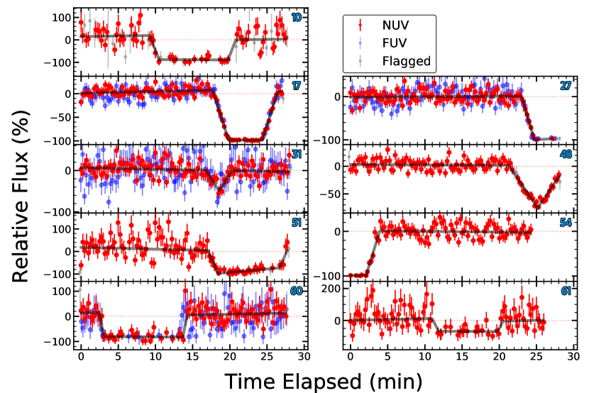
Figure 4: Light curves for the nine eclipsing sources in our sample. WD ID# from Table 2 is given in the top right of each panel. When available, FUV data is overplotted in blue and flagged points are plotted in gray. We fit simple trapezoidal eclipse models (black) to estimate eclipse duration and center, which are given in Table 4.

One known eclipsing binary is included in our sample, US 3566 (2MASS J03030835$+$0054438, ID# 10), which was spectroscopically characterized as a WD and M4-dwarf (DC+dM4) binary system with an orbital period of $3.2$ hours (Eisenstein et al., 2006; Pyrzas et al., 2009). Debes et al. (2012) classified the system as a post-common-envelope binary with infrared excess, at $3\mu$m using WISE infrared observations. Follow-up observations show that the white dwarf in the system is strongly magnetic (8 MG) and that this IR excess is due to cyclotron emission; this pre-cataclysmic variable will likely evolve into an intermediate polar in roughly 1 Gyr (Parsons et al., 2013).

There are five GALEX observations of US 3566, two of which show a partial-duration and a full-duration eclipse, plotted in Figure 4. The gap in GALEX observations prevents further refinement of the US 3566 orbital parameters presented in Eisenstein et al. (2006).

5 New Pulsators

Out of the 63 variables detected, we find 41 new WD pulsators in our sample which are outlined in Table 2. Light curves for the highest ranked visit of each source are plotted in Appendix B. The new pulsators detected have a median Gaia $G=18.0$ mag. Figure 3 compares the distribution of new pulsator magnitudes to known DA pulsators listed in Table 4 of Bognar & Sodor (2016). Many bright sources that might be traditional candidates for variability are overexposed in the GALEX aperture, leading to dither effects and high flag ratios of $>25\%$. There are a number of known pulsators in which we do not detect variation due to overexposure and other instrumental effects.

One way pulsators can be distinguished spectroscopically is by consideration of their $\log g$ and $T_{\rm{eff}}$, given their location in an instability strip (Figure 35, Gianninas et al., 2011). We construct a similar parameter space in a Gaia DR2 color-magnitude diagram (CMD) in Figure 2. Both the DAV and DBV instability strips occupy distinct locations on the Gaia CMD. We find most pulsators fall into the DAV instability strip, labeled in Figure 2; this is expected since more than 80 percent of white dwarfs in magnitude-limited samples have hydrogen-dominated atmospheres (Kleinman et al., 2013). These WDs could also be photometrically variable due to surface spots, as in hot DQVs (Williams et al., 2016). However, the pulse shapes and Gaia CMD positions suggest the variations are due to pulsations and not rotationally driven spots.

We include spectra for two new pulsators in Appendix A showing expected H/He spectral features. We emphasize that we did not search for variability based on CMD location. Thus, sources falling in known instability strips provides additional confidence in our method and their classification.

5.1 WD J212402.03$-$600100.05: A New Massive Pulsator

This pulsator, ID #52, has an absolute Gaia G magnitude roughly $1$ mag fainter than the rest of the DAVs (Figure 2). This is likely a more massive WD pulsator, similar to GD 518 (Hermes et al., 2013), since WDs decrease in radius with increasing mass. Hydrogen-atmosphere model fits of the Gaia CMD position suggest this is a roughly $12510\pm 750$ K WD with a mass of $1.16\pm 0.04$ $\text{M}_{\odot}$ (Gentile Fusillo et al., 2018). Massive WD pulsators are of particular interest since the cores can be oxygen/neon or crystallized. Additional follow up photometric and spectroscopic observations and classification will be presented in an upcoming paper.

5.2 WD J162724.72$+$392027.25

One DA pulsator, ID #43, is $\sim 0.2$ mag redder than the rest of the population. Based on the light curves presented in Appendix 10, we are confident the variability detected is due to pulsations. Inspecting the Pan-STARRS images (Chambers et al., 2016; Flewelling et al., 2016) of this WD, there is a relatively bright red star ($r\sim 13.6$ mag, $g-r\sim 0.7$ mag) approximately $2^{\prime\prime}$ away from the WD. Considering the Gaia point spread functions extend out to $1$-$2^{\prime\prime}$ (Fabricius et al., 2016), the redward shift of ID #43 compared to the rest of the DAV population is likely due to blending of these sources. Thus, we still consider this object a new DAV pulsator despite its anomalous location in Figure 2.

5.3 DB Pulsators

The CMD is also helpful in identifying non-DAV pulsators our variability sample. One of the known pulsators detected, GD 358, (ID #45), is a known DBV pulsator (Kotak et al., 2003). We find two new pulsators that are spectroscopically known to be DB type WDs, ID#22 and #32, as well as two others with unknown spectral types, ID#9 and #35, that occupy a similar parameter space as GD 358 on the CMD. Therefore, we classify these four new pulsators as new DB pulsators (DBVs).

6 New Eclipsing WDs

We detect eight new eclipsing binaries in addition to the pulsators. These WDs are overluminous in the Gaia CMD (Figure 2), suggesting the excess flux is from their companions. For the three sources that are known spectroscopic binary systems, we present the first evidence of eclipses (ID#27, 31, and 60, Silvestri et al., 2006; Eisenstein et al., 2006; Kepler et al., 2015). The light curves for all eclipsing sources are plotted in Figure 4.

Two of the eclipses detected (ID#31, 48) are grazing eclipses, where the drop in flux is not consistent with $100\%$ decrease in flux. There are also two eclipses that are partially observed (ID#27, 54). Though we are limited by the short timescales of GALEX observations, we construct simple trapezoidal eclipse models to estimate eclipse duration and center. The results of these fits are reported in Table 4.

Table 4: Data on eclipsing WDs in our survey. Parameters are derived using trapezoidal transit fits. Eclipse center is given in minutes from observation start.

ID	Obs Start	Eclipse Center	Duration
	(TDB JD)	(min from start)	(min)
10	2455164.301501	$15.01^{+0.21}_{-0.42}$	$11.56^{+0.96}_{-0.82}$
17	2453436.107338	$22.06^{+0.06}_{-0.06}$	$8.80^{+0.17}_{-0.20}$
27	2453027.340377	–	$\gtrsim 4$
31	2454946.159964	$18.54^{+0.13}_{-0.08}$	$3.45^{+0.84}_{-0.49}$
48	2455387.297459	$25.16^{+0.06}_{-0.07}$	$6.74^{+0.51}_{-0.39}$
51	2455039.073697	$23.29^{+0.60}_{-0.30}$	$12.48^{+1.19}_{-0.60}$
54	2453254.882559	–	$\gtrsim 3$
60	2454716.101505	$8.35^{+0.10}_{-0.09}$	$11.83^{+0.41}_{-0.29}$
61	2455468.906436	$15.73^{+0.15}_{-0.18}$	$9.55^{+0.38}_{-0.34}$

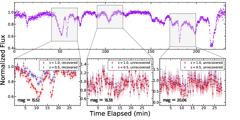
Figure 5: Examples of light curve injection for three WDs (PG 0846+558, WD J095143.98$+074956.31$, and US 3608 from left to right) with two scale factors, $s=1.0$ and $s=0.5$. NUV magnitudes are given in the bottom left of each panel.

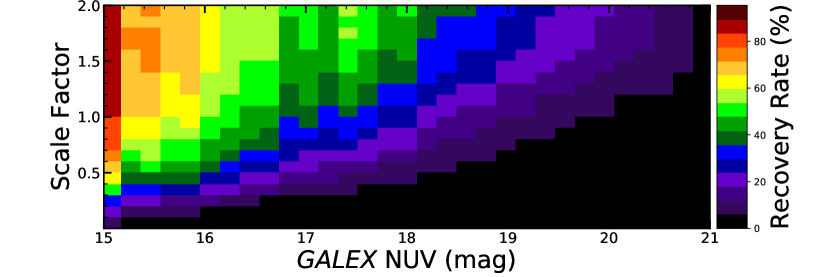
Figure 6: Recovery percentage as a function of GALEX NUV magnitude and scale factor. As expected, there is a higher recovery rate for larger scales and brighter sources.

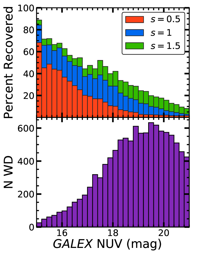
Figure 7: Top: Recovery percentage as a function of magnitude for three selected scale factors. Bottom: Number of GALEX WDs included in the injection recovery sample for each $0.2$ magnitude bin.

7 Non-Detection of Planetary Debris Transits

Despite potential disruption during stellar evolution, a significant fraction of wide planetary systems are expected to survive evolution through the Asymptotic Giant Branch (Mustill & Villaver, 2012). Observations of debris disks and IR excesses (e.g., Barber et al., 2012; Rocchetto et al., 2015), as well as abundances consistent with bulk Earth accreted material (e.g., Gänsicke et al., 2012), provide strong evidence of rocky debris around WDs. Yet direct evidence of transiting planetesimals/asteroids has only been found in WD 1145+017 (Vanderburg et al., 2015; Gänsicke et al., 2016; Izquierdo et al., 2018; Karjalainen et al., 2019). This source has multiple orbiting bodies with trails of debris, resulting in multiple broad periodogram peaks. Using 1148 K2 WDs, the occurrence rate of transiting material was estimated to be $\sim 12\%$ (van Sluijs & Van Eylen, 2018). Though we expect our methodology described in §3 to detect transiting objects, time-series photometry of GALEX WDs does not reveal any such sources. To test recovery of transiting debris, we perform injections of transits from the WD 1145+017 light curve (Gänsicke et al., 2016, Figure 1).

7.1 Source Selection

From our initial sample of 23,676 WDs, we include only GALEX observations with $>500$ seconds of exposure. This cutoff is based on our detected WD variables, which all have exposure of $>700$ seconds. We also exclude any WDs with rank in the top 5% of sources, as calculated in §3. Additionally, we do not consider any WDs included in the K2 study from van Sluijs & Van Eylen (2018), allowing a comparison between independent samples. Since many bright sources are overexposed in the GALEX aperture, we limit the brightness at $15$ GALEX NUV magnitude. These cuts leave $15034$ WDs in our injection-recovery sample.

To test recovery, we inject portions of the 3.9 hour optical light curve of WD 1145+017 presented in Gänsicke et al. (2016) and shown in the top panel of Figure 5. This light curve has a large range of transit depths and durations, as well as periods of no variability. Since our GALEX observations have maximum exposures of 30 minutes, we inject a wide variety of possible transits.

In the first step of the recovery procedure, we iterate through NUV magnitude bins of width $0.2$ mag. A random WD in the magnitude bin is selected from the trimmed sample. If the selected WD has more than one GALEX observation, we randomly select a single observation from the set. A segment of the optical light curve is then selected at random, matching the duration of the GALEX observation.

After selecting an optical light curve segment to inject, we multiply the optical flux by a scale factor from 0–2, also chosen at random. If we select random 30-minute segments of the WD 1145+017 LC, 90% have a depth $>10\%$ in flux, $\sim 45\%$ have a depth $>25\%$, and $\sim 8\%$ have a depth $>50\%$. The inclusion of a scale factor allows for a wider sampling of possible transit depths, while still remaining true to the distinct patterns of variability observed in WD 1145+017.

Finally, using the methodology described in §3, we compute the rank for this observation after injection. Though we had visually inspected the top 10% of ranked sources in our variability search, we conservatively consider an injected source recovered if the new rank falls within the top 5% of ranks computed for all WDs.

Figure 5 plots an example of injections at three magnitudes and two scale factors. The recovery of a source is not only dependent on the section of the WD 1145+017 optical light curve selected and the scale factor used, but also the magnitude of the source. For fainter sources, the increased scatter masks out injected transits, limiting recovery potential.

7.2 Recovery Results

We run the injection/recovery routine with $2\text{\times}{10}^{5}\text{\,}\mathrm{i}$terations per 0.2 magnitude bin. With a scale factor bin size of 0.1, there are $\sim 10^{4}$ iterations at each magnitude and scale factor bin. Figure 6 plots the recovery percentage for each bin. As expected, recovery percentage is higher for larger scales and brighter sources. Figure 7 plots the recovery percentage at three selected scale factors and a histogram of source magnitudes.

Due to the low number of bright sources, there are larger fluctuations in recovery percentage between adjacent magnitude bins of $\lesssim 17.5$ NUV mag. Overexposure and higher flag counts also cause more variation in the quality of these bright GALEX observations. Comparison of the three sources in Figure 5 demonstrates a greater change in noise between the 15.52 and 18.38 mag sources then the 18.38 and 20.06 mag sources.

To estimate the number of WDs for which we can rule out transiting debris, we consider the number of WDs in a given magnitude bin, shown in the bottom panel of Figure 7, multiplied by the recovery rate at a chosen scale factor:

$$N_{\text{excluded,}s}=\sum_{m=15}^{21}N_{m}\times R_{m,s}$$ (7)

where $m$ is the GALEX NUV magnitude, $N_{m}$ is the number of sources used for injection in the $m^{\text{th}}$ magnitude bin (Figure 7), and $R_{m,s}$ is the recovery fraction calculated at the corresponding magnitude and scale factor (Figure 8). This value represents the estimated number of WDs excluded from hosting detectable transits. To place an upper limit on the occurrence rate of transiting debris, we consider a binomial population where a detected transit is considered a “success". Since no transiting objects are present in our sample, we use the equal-tailed Jeffreys Interval to estimate a $3\sigma$ upper limit of zero successes in $N_{\text{excluded}}$ trials.

Figure 8 plots $N_{\text{excluded}}$ and the resulting $3\sigma$ occurrence upper limits as a function of the scale factor. Under the assumption the material is opaque, we calculate our $3\sigma$ upper limits at a scale factor of $s=1.0$. We find 1024 WDs are ruled out from having transiting debris in our study, leading to a $3\sigma$ occurrence rate upper limit on transiting debris around WDs of 0.5%. We emphasize that this limit does not describe the occurrence rate of debris, but the rate of transiting debris given non-detections in GALEX photometry. The full results of the occurrence rate calculation for all scale factors are provided as supplementary material.

This occurrence rate does not take into account recovery of different body sizes or orbital separations, only the detection of transiting debris analogous to WD 1145+017. Using 1148 WDs from K2, combined with an estimated transit probability of 2% (Vanderburg et al., 2015), van Sluijs & Van Eylen (2018) reported a 12% occurrence rate with 95% confidence bounds spanning 1-45%. Taking the same consideration into account, our calculated occurrence rate is consistent with that of van Sluijs & Van Eylen (2018). The true occurrence rate of these systems also depends on the observed inclination, modifying our upper limit by a factor of $\cos(i)$, as well as the UV-to-optical scale ratio of the transit depths. Even if the transits are half as deep in the UV ($s=0.5$), our $3\sigma$ occurrence rate upper limit is still $<$2% (see Figure 8).

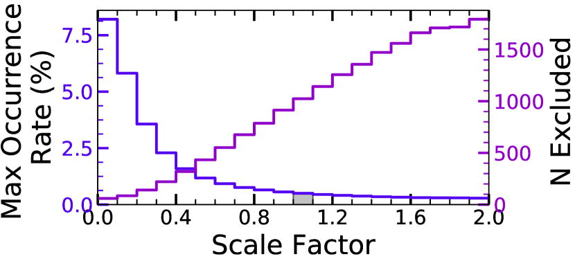
Figure 8: Maximum $3\sigma$ occurrence rates of transiting debris calculated for each scale factor. The number of sources excluded from hosting transiting sources at each scale factor is given along the right axis calculated using Equation 7. We take the maximum occurrence rate, 0.5%, to be the $3\sigma$ upper limit at a scale factor of 1.0 (§7.2).

8 Conclusions

We present the largest UV photometric WD survey to-date in a search for new variable WDs. Our sample of 23,676 WDs comes from four separate catalogs, which was trimmed based on GALEX exposure time. We demonstrate the application of short baseline GALEX observations for the detection of photometric variability.

Applying a system of weighted metrics results in the detection of 37 new DA pulsators and four new DB pulsators. We provide the first eclipse detection of eight eclipsing WD binary systems. Appendix B plots light curves of all new pulsators and Figure 4 plots the nine eclipsing sources. Using Gaia color information, we classify these pulsators as either DAV or DBV using a CMD (Figure 2). Included in our new pulsators is the detection of a new massive pulsator, WD J212402.04$-$600100.05 (Gaia $G$=18.0 mag), of which we are currently conducting follow-up observations.

We detect variability in sources up to 20th $G$-band apparent magnitude, with a median of $\sim 18^{\rm{th}}$ magnitude. GALEX/gPhoton are more successful in searching for fainter pulsators, as compared to the known population (Bognar & Sodor, 2016). This is partially due to oversaturation of bright sources in the GALEX aperture, preventing the detection of some known pulsators. For sources where observations were taken in FUV and NUV bands, there is consistent pulsation variability timescales in each. By considering multiple metrics to identify variability, we are also able to identify pulsations and eclipses when only one band is available.

While this study provides a comprehensive analysis of GALEX WD photometry, there are almost certainly additional low amplitude variability candidates to be found around fainter sources. This study does not provide any estimates on detectability or occurrence rates of WD pulsators. There are also some sources where detection is limited by instrumental effects, most notably the telescope dither and oversaturation of the GALEX aperture.

Though our method of variability selection did not return any candidates for transiting exoplanet debris, detection of these sources could still be possible with time-series photometry of GALEX observations. For sources with multiple visits, it is feasible to detect multi-periodic transits, similar to those detected by Vanderburg et al. (2015). We perform synthetic injections of the WD-1145+017 light curve from Figure 1 of Gänsicke et al. (2016) and use the system of weighted metrics to assess recovery. We find the maximum $3\sigma$ occurrence rate of WD 1145+017-like transiting objects to be 0.5%.

Both pulsators and eclipsing binary sources presented here are potential targets for longer-baseline studies. Timing of detected pulsation modes can be used for asteroseismology. Detection and classification of these sources is a continuation in probing WD interiors to better understand the final stage of stellar evolution for the majority of stars.

Appendix A New WD Pulsator Spectra

Using the SuperNova Integral Field spectrograph (Lantz et al., 2004, SNIFS) on the University of Hawaii 88-inch telescope (UH88), we present spectroscopic observations for two of the new pulsators. These spectra were taken to confirm our classification of the new DA/B pulsators via the Gaia CMD (Figure 2). The spectra cover roughly 3200–9000Å, excluding the dichroic crossover ($\sim$5000–5200Å).

The spectrum for WD J003116.51$+$474828.39 (ID#2), provided in the top panel of Figure 9, was taken on MJD 58301.584757 with an exposure time of 1820 seconds at an airmass of 1.272. The spectrum exhibits broad H absorption lines, notably at 4340, 4861, and 6563Å, confirming our initial DAV classification.

The spectrum for WD J132952.63$+$392150.8 (ID#35), provided in the bottom panel of Figure 9, was taken on MJD 58321.301690 with an exposure time of 1520 seconds at an airmass of 1.480. The spectrum exhibits He I features at 4471, 4712, 5876, and 6678Å, again confirming our DBV classification.

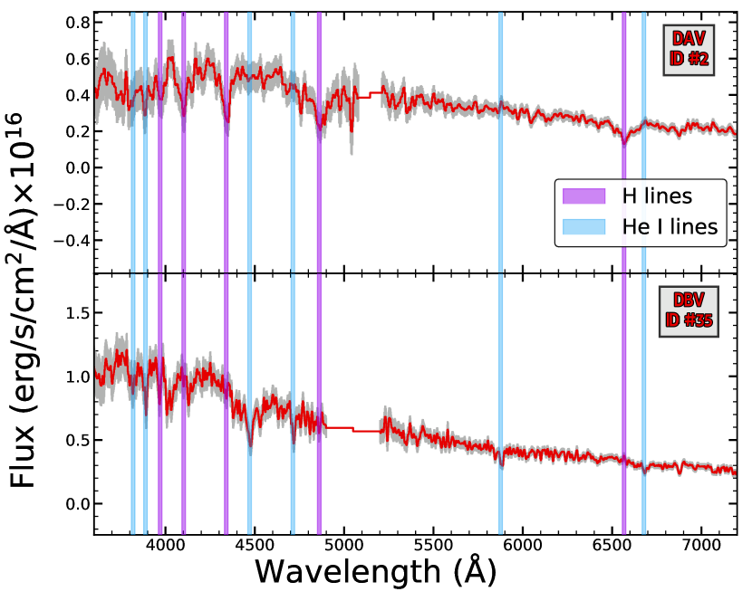
Figure 9: UH88/SNIFS spectra for two new pulsators with error bars in gray. Top: DAV pulsator with H absorption lines. Bottom: DBV pulsator with He absorption lines. These spectra confirm our classifications based on the Gaia CMD in Figure 2.

Appendix B Pulsator Light Curves

We create UV lightcurves for all detected pulsators presented in this study in Figure 10. When available, NUV and FUV data are plotted, in red and blue, respectively. For cases where there are more than one visit displaying variability, we plot the highest ranked light curve. As expected (Kepler et al., 2000), we see larger amplitude variability in the FUV.

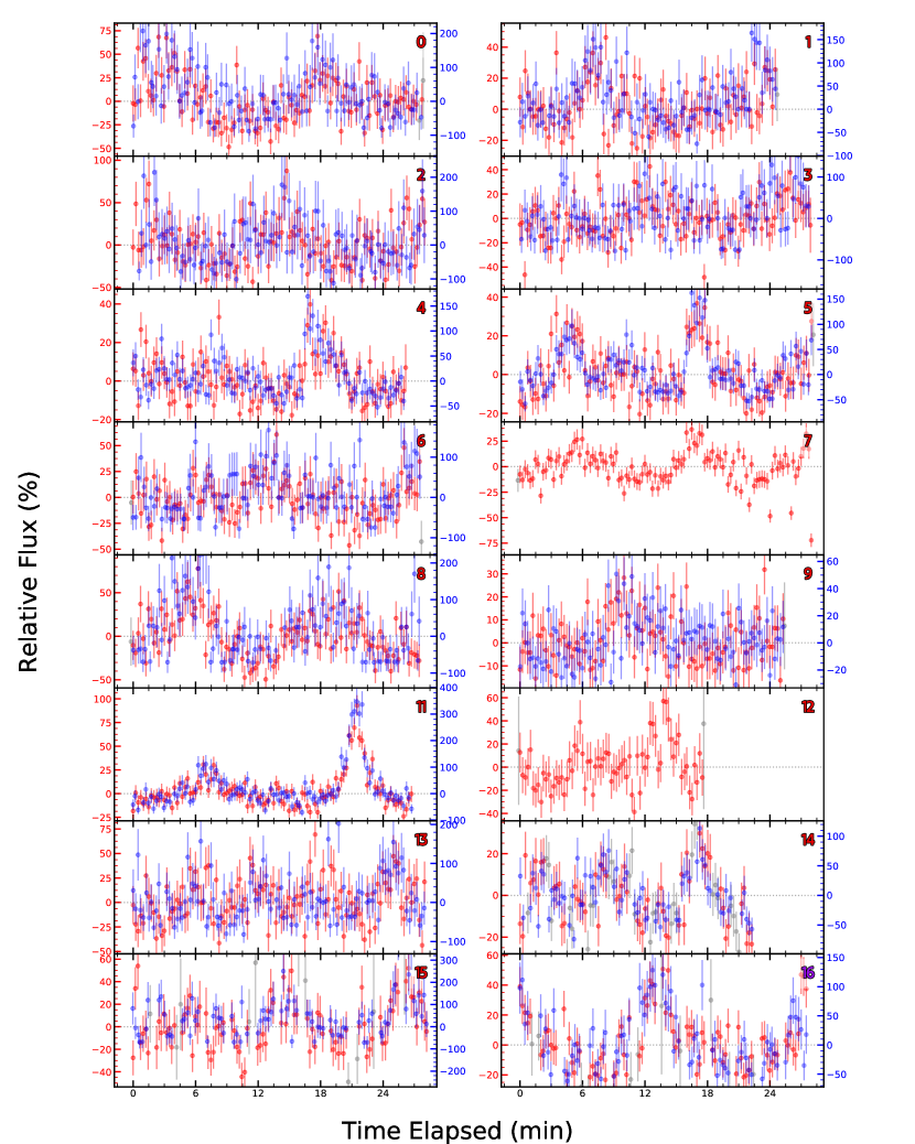
Figure 10: Light curves for all pulsators detected in our survey. ID numbers from Table 2 are given in top right of each panel, with new pulsators in red and known pulsators in purple. NUV data is plotted in red, FUV in blue, and flagged points in gray.

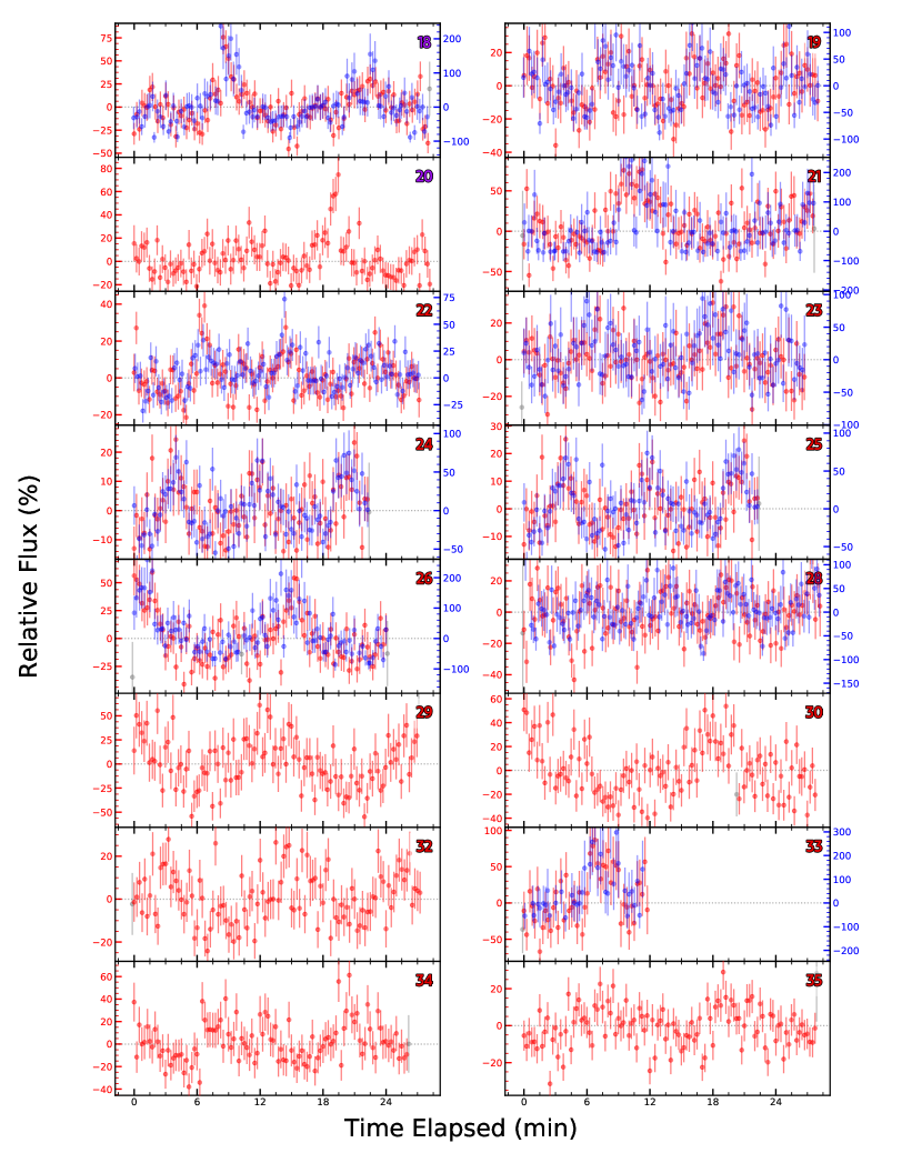
Figure 11: Continuation of Figure 10

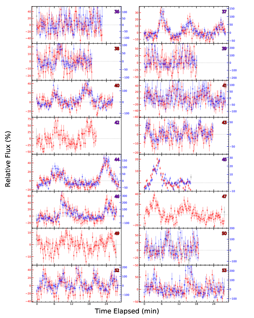
Figure 12: Continuation of Figure 10

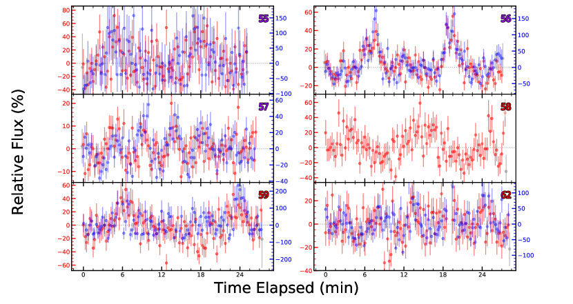
Figure 13: Continuation of Figure 10

References

- Althaus et al. (2010) Althaus L. G., Córsico A. H., Isern J., García-Berro E., 2010, Astronomy and Astrophysics Review, 18, 471
- Baluev (2008) Baluev R. V., 2008, MNRAS, 385, 1279
- Barber et al. (2012) Barber S. D., Patterson A. J., Kilic M., Leggett S. K., Dufour P., Bloom J. S., Starr D. L., 2012, ApJ, 760, 26
- Bognar & Sodor (2016) Bognar Z., Sodor A., 2016, Information Bulletin on Variable Stars, 6184, 1
- Brown et al. (2017) Brown W. R., Kilic M., Kosakowski A., Gianninas A., 2017, ApJ, 847, 10
- Castanheira et al. (2007) Castanheira B. G., et al., 2007, A&A, 462, 989
- Castanheira et al. (2010) Castanheira B. G., Kepler S. O., Kleinman S. J., Nitta A., Fraga L., 2010, MNRAS, 405, 2561
- Catalán et al. (2008) Catalán S., Isern J., García-Berro E., Ribas I., 2008, MNRAS, 387, 1693
- Chambers et al. (2016) Chambers K. C., et al., 2016, preprint, p. arXiv:1612.05560 (arXiv:1612.05560)
- Córsico (2017) Córsico A. H., 2017, preprint, p. arXiv:1703.00934 (arXiv:1703.00934)
- Debes et al. (2012) Debes J. H., Hoard D. W., Farihi J., Wachter S., Leisawitz D. T., Cohen M., 2012, ApJ, 759, 37
- Dufour et al. (2017) Dufour P., Blouin S., Coutu S., Fortin-Archambault M., Thibeault C., Bergeron P., Fontaine G., 2017, in 20th European White Dwarf Workshop. p. 3
- Eisenstein et al. (2006) Eisenstein D. J., et al., 2006, The Astrophysical Journal Supplement Series, 167, 40
- Fabricius et al. (2016) Fabricius C., et al., 2016, A&A, 595, A3
- Faedi et al. (2011) Faedi F., West R. G., Burleigh M. R., Goad M. R., Hebb L., 2011, Monthly Notices of the Royal Astronomical Society, 410, 899
- Farihi (2016) Farihi J., 2016, New Astron. Rev., 71, 9
- Flewelling et al. (2016) Flewelling H. A., et al., 2016, preprint, p. arXiv:1612.05243 (arXiv:1612.05243)
- Fontaine & Brassard (2008) Fontaine G., Brassard P., 2008, PASP, 120, 1043
- Fontaine et al. (2001) Fontaine G., Bergeron P., Brassard P., Billères M., Charpinet S., 2001, ApJ, 557, 792
- Fulton et al. (2014) Fulton B. J., et al., 2014, ApJ, 796, 114
- Gaia Collaboration et al. (2018) Gaia Collaboration Brown A. G. A., Vallenari A., Prusti T., de Bruijne J. H. J., Babusiaux C., Bailer-Jones C. A. L., 2018, preprint, p. arXiv:1804.09365 (arXiv:1804.09365)
- Gänsicke et al. (2012) Gänsicke B. T., Koester D., Farihi J., Girven J., Parsons S. G., Breedt E., 2012, MNRAS, 424, 333
- Gänsicke et al. (2016) Gänsicke B. T., et al., 2016, ApJ, 818, L7
- Gentile Fusillo et al. (2017) Gentile Fusillo N. P., et al., 2017, MNRAS, 469, 621
- Gentile Fusillo et al. (2018) Gentile Fusillo N. P., et al., 2018, preprint, p. arXiv:1807.03315 (arXiv:1807.03315)
- Gianninas et al. (2011) Gianninas A., Bergeron P., Ruiz M. T., 2011, ApJ, 743, 138
- Hermes et al. (2013) Hermes J. J., Montgomery M. H., Mullally F., Winget D. E., Bischoff-Kim A., 2013, ApJ, 766, 42
- Hermes et al. (2017) Hermes J. J., et al., 2017, ApJS, 232, 23
- Izquierdo et al. (2018) Izquierdo P., et al., 2018, MNRAS, 481, 703
- Karjalainen et al. (2019) Karjalainen M., de Mooij E. J. W., Karjalainen R., Gibson N. P., 2019, MNRAS, 482, 999
- Kepler et al. (2000) Kepler S. O., Robinson E. L., Koester D., Clemens J. C., Nather R. E., Jiang X. J., 2000, ApJ, 539, 379
- Kepler et al. (2015) Kepler S. O., et al., 2015, MNRAS, 446, 4078
- Kepler et al. (2016) Kepler S. O., et al., 2016, MNRAS, 455, 3413
- Kleinman et al. (2013) Kleinman S. J., et al., 2013, ApJS, 204, 5
- Koester & Chanmugam (1990) Koester D., Chanmugam G., 1990, Reports on Progress in Physics, 53, 837
- Kotak et al. (2003) Kotak R., van Kerkwijk M. H., Clemens J. C., Koester D., 2003, A&A, 397, 1043
- Lantz et al. (2004) Lantz B., et al., 2004, in Mazuray L., Rogers P. J., Wartmann R., eds, Vol. 5249, Optical Design and Engineering. pp 146–155, doi:10.1117/12.512493
- Lomb (1976) Lomb N. R., 1976, Ap&SS, 39, 447
- Martin et al. (2005) Martin D. C., et al., 2005, ApJ, 619, L1
- Million et al. (2016) Million C., et al., 2016, ApJ, 833, 292
- Morrissey (2006) Morrissey P., 2006, in Society of Photo-Optical Instrumentation Engineers (SPIE) Conference Series. p. 62660Y, doi:10.1117/12.671839
- Morrissey et al. (2005) Morrissey P., et al., 2005, ApJ, 619, L7
- Mukadam et al. (2004) Mukadam A. S., et al., 2004, ApJ, 607, 982
- Mullally et al. (2005) Mullally F., Thompson S. E., Castanheira B. G., Winget D. E., Kepler S. O., Eisenstein D. J., Kleinman S. J., Nitta A., 2005, in 14th European Workshop on White Dwarfs. p. 581
- Mustill & Villaver (2012) Mustill A. J., Villaver E., 2012, ApJ, 761, 121
- Nitta et al. (2009) Nitta A., et al., 2009, ApJ, 690, 560
- Ochsenbein et al. (2000) Ochsenbein F., Bauer P., Marcout J., 2000, Astronomy and Astrophysics Supplement Series, 143, 23
- Parsons et al. (2013) Parsons S. G., Marsh T. R., Gänsicke B. T., Schreiber M. R., Bours M. C. P., Dhillon V. S., Littlefair S. P., 2013, MNRAS, 436, 241
- Parsons et al. (2015) Parsons S. G., et al., 2015, MNRAS, 449, 2194
- Pyrzas et al. (2009) Pyrzas S., et al., 2009, in Journal of Physics Conference Series. p. 012028, doi:10.1088/1742-6596/172/1/012028
- Rocchetto et al. (2015) Rocchetto M., Farihi J., Gänsicke B. T., Bergfors C., 2015, MNRAS, 449, 574
- Scargle (1982) Scargle J. D., 1982, ApJ, 263, 835
- Silvestri et al. (2006) Silvestri N. M., et al., 2006, AJ, 131, 1674
- Stobie et al. (1995) Stobie R. S., O’Donoghue D., Ashley R., Koen C., Chen A., Kilkenny D., 1995, MNRAS, 272, L21
- Toonen et al. (2017) Toonen S., Hollands M., Gänsicke B. T., Boekholt T., 2017, A&A, 602, A16
- Tremblay et al. (2015) Tremblay P. E., Gianninas A., Kilic M., Ludwig H. G., Steffen M., Freytag B., Hermes J. J., 2015, ApJ, 809, 148
- Tucker et al. (2018) Tucker M. A., et al., 2018, MNRAS, 475, 4768
- VanderPlas (2018) VanderPlas J. T., 2018, The Astrophysical Journal Supplement Series, 236, 16
- Vanderburg et al. (2015) Vanderburg A., et al., 2015, in AAS/Division for Extreme Solar Systems Abstracts. p. 502.02
- Voss et al. (2006) Voss B., Koester D., Østensen R., Kepler S. O., Napiwotzki R., Homeier D., Reimers D., 2006, A&A, 450, 1061
- Welch & Stetson (1993) Welch D. L., Stetson P. B., 1993, AJ, 105, 1813
- Wenger et al. (2000) Wenger M., et al., 2000, Astronomy and Astrophysics Supplement Series, 143, 9
- Williams et al. (2016) Williams K. A., Montgomery M. H., Winget D. E., Falcon R. E., Bierwagen M., 2016, ApJ, 817, 27
- Winget & Kepler (2008) Winget D. E., Kepler S. O., 2008, Annual Review of Astronomy and Astrophysics, 46, 157
- de la Vega & Bianchi (2018) de la Vega A., Bianchi L., 2018, preprint, (arXiv:1808.10455)
- van Sluijs & Van Eylen (2018) van Sluijs L., Van Eylen V., 2018, MNRAS, 474, 4603