Topology Controlled Potts Coarsening

Abstract

We uncover unusual topological features in the long-time relaxation of the $q$-state kinetic Potts ferromagnet on the triangular lattice that is instantaneously quenched to zero temperature from a zero-magnetization initial state. For $q=3$, the final state is either: the ground state (frequency $\approx 0.75$), a frozen three-hexagon state (frequency $\approx 0.16$), a two-stripe state (frequency $\approx 0.09$), or a three-stripe state (frequency $<2\times 10^{-4}$). Other final state topologies, such as states with more than 3 hexagons, occur with probability $10^{-5}$ or smaller, for $q=3$. The relaxation to the frozen three-hexagon state is governed by a time that scales as $L^{2}\ln L$. We provide a heuristic argument for this anomalous scaling and present additional new features of Potts coarsening on the triangular lattice for $q=3$ and for $q>3$.

I Introduction

When a ferromagnet with multiple degenerate ground states is quenched from above to below its critical point, a coarsening domain mosaic emerges in which distinct phases compete to prevail in the ordering dynamics Gunton et al. (1982); Bray (2002). In contradiction to continuum theories of coarsening, which predict that the ground state is ultimately reached, the long-time states that persist in discrete spin systems can be surprisingly rich when the quench is to zero temperature, $T\!=\!0$. Such states are actually metastable but infinitely long lived when this quench to $T\!=\!0$ is instantaneous. These persistent states may be static and geometrically simple, such as stripe states in the kinetic Ising ferromagnet in spatial dimension $d=2$ Spirin et al. (2001a, b). An unexpected and simplifying feature of these stripe configurations is that their occurrence probabilities can be computed exactly in terms of the spanning probabilities of continuum percolation Barros et al. (2009); Olejarz et al. (2012); Blanchard and Picco (2013); Cugliandolo (2016); Blanchard et al. (2017); Yu (2017).

In contrast, for the $d=3$ kinetic Ising ferromagnet, these persistent states are often topologically complex and non-stationary Olejarz et al. (2011a, b). An even more striking feature of the $d=3$ Ising ferromagnet is that the probability to reach the ground state rapidly decreases with $L$ and realizations that do reach the ground states play an insignificant role for large $L$. Almost always, the final state consists of two, and only two, clusters—one spin up and one spin down. These two clusters are intertwined so that each cluster typically has a high genus. On the surfaces of these clusters, there are a small but finite fraction of “blinker” spins—spins in which three neighbors are in the spin-up state and three neighbors are in the spin-down state. Consequently, blinkers can freely flip between the spin-up and spin-down states with no energy cost.

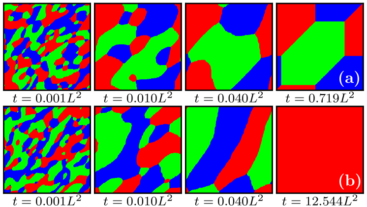
Figure 1: Realizations of zero-temperature coarsening in the $3$-state Potts ferromagnet on a periodically bounded triangular lattice of linear dimension $L=384$ that freeze into (a) a static three-hexagon state and (b) the ground state after evolving through a long-lived off-axis three-hexagon configuration.

The domain geometry that arises when the kinetic $q$-state Potts ferromagnet is instantaneously quenched to zero temperature is richer still Safran et al. (1982, 1983); Sahni et al. (1983a, b); Grest et al. (1988); Ferrero and Cannas (2007); de Oliveira (2009); LACS10 ; LAC12 . The Potts system has been extensively investigated because of its applications to diverse coarsening phenomena, such as soap froths Glazier et al. (1990); Thomas et al. (2006); D.Weaire and Rivier (2009), magnetic domains Srolovitz et al. (1984); Fradkov and Udler (1994); Raabe (2000); Zöllner (2011); Babcock et al. (1990); Jagla (2004), cellular tissue and other natural tilings Mombach et al. (1990, 1993); Hočevar et al. (2010). For $T=0$ quenches, the ground state is rarely reached for large $q$ de Oliveira et al. (2004a, b) and “blinker” (freely flippable) spins arise on the square lattice Olejarz et al. (2013). A domain mosaic on the square lattice may also get stuck in a nearly static, geometrically complex state for times that are much larger than the coarsening time scale. This metastability is eventually, but not always, disrupted by a macroscopic avalanche in which either a lower-energy geometrically complex state or the ground state is reached Olejarz et al. (2013).

In this work, we investigate intriguing and apparently overlooked features of the coarsening of the 3-state Potts ferromagnet on the triangular lattice. Our two main results are: (a) When quenched to $T=0$, roughly 75% of all trajectories end in the ground state, 16% in an unexpected frozen three-hexagon state (Fig. 1(a)), 9% in a two-stripe state, and a tiny fraction in a three-stripe state; the probability to reach more complex geometries, such as frozen states with more than three hexagons, is of the order of $10^{-5}$. (b) The approach to the final states is governed by three distinct time scales: (i) the conventional coarsening time $L^{2}$, with $L$ the linear dimension of the system, (ii) a time that appears to grow as $L^{2}\ln L$, which governs the approach to frozen three-hexagon states, and (iii) a time that grows roughly as $L^{3.5}$, which governs the relaxation of off-axis three-hexagon states or diagonal stripe states to the ground state. These results will be presented in the following sections.

II Triangular 3-State Potts Ferromagnet

It is convenient to represent the triangular lattice as a periodically bounded square array with additional diagonal interactions to the upper-right and lower-left next-nearest neighbors (on the square lattice). It is worth mentioning that this periodic system cannot be wrapped onto a two-dimensional torus. The Hamiltonian of the system is defined as

$$\mathcal{H}=-2J\sum_{i,j}\big{[}\delta(s_{i},s_{j})-1\big{]}\,,$$ (1)

where $\delta(a,b)$ is the Kronecker delta function, and the sum runs over all nearest-neighbor spin pairs $i,j$. In this representation, each misaligned spin pair contributes $+2J$ to the energy, while each aligned pair contributes zero. We choose the coupling strength $J$ to be equal to 1 by measuring all energies in units of $J$.

We use the following simple $T=0$ single spin-flip dynamics: flip events that decrease or conserve the systems energy are accepted with probability $1$ Sahni et al. (1983a); Bortz , while flip events that increase the energy have zero probability of occurring. We use an event-driven algorithm to implement this dynamics in a rejection-free manner Sahni et al. (1983a); Bortz . Spins are categorized into classes $k$, that are labeled by the number $F_{k}$ of distinct permissible flip events that spins in this class may undergo. The total weight of each class is $W_{k}=F_{k}N_{k}$, where $N_{k}$ is the number of spins in the $k^{\rm th}$ class. To flip a spin, we select a class with a probability proportional to its weight $W_{k}$ and allow a randomly chosen member spin to flip to any energetically allowed spin state with unit probability. The time is then incremented by $\Delta t=-\ln(r)/\sum_{k}{F_{k}}$, where $r$ is a uniform random number on the interval $(0,1)$, and the summation is over the total number of permissible flips in the system at the time of the event. We then update the lists of spins in each class.

We simulate systems of linear dimension $L$ between 12 and 384, with $10^{5}$ realizations for each size. We choose an initial condition that is either a random zero-magnetization state or an antiferromagnetic state. Both give virtually identical results and we henceforth restrict ourselves to the antiferromagnetic initial condition for simplicity. In this case, we only need to average over trajectories of the spin state of the system, rather than averaging over many spin-state trajectories and also many initial conditions.

III Time Dependence of the Relaxation

In the conventional picture of phase-ordering kinetics, a finite system of linear dimension $L$ that is prepared in a random initial state and then instantaneously quenched to $T=0$ will eventually reach the ground state in a time that grows with system size as $L^{2}$ Gunton et al. (1982); Bray (2002). We therefore expect that the probability $S(t)$ that the system has not yet reached the ground state at time $t$, which we define as the “survival” probability, will decay exponentially with time, $S(t)\sim e^{-t/\tau(L)}$, with an associated relaxation time $\tau(L)$ that grows as $L^{2}$. Equivalently, $S(t)$ can be viewed as probability that flippable spins still exists at time $t$. Very different relaxation occurs in the kinetic 3-state Potts ferromagnet on the triangular lattice. Here, the time dependence of $S(t)$ appears to be governed by at least three distinct time scales (Fig. 2).

For this Potts system, the survival probability decays to zero for all realizations in a finite time; the longest lifetime in $10^{5}$ realizations for $L=384$ is $29.989\,L^{2}$. This inertness of all final states also arises in the kinetic Ising ferromagnet on the square lattice. A static final state contrasts with the kinetic Potts ferromagnet on the square lattice, where blinker spins persist and $S(t)$ never decays to zero Olejarz et al. (2013).

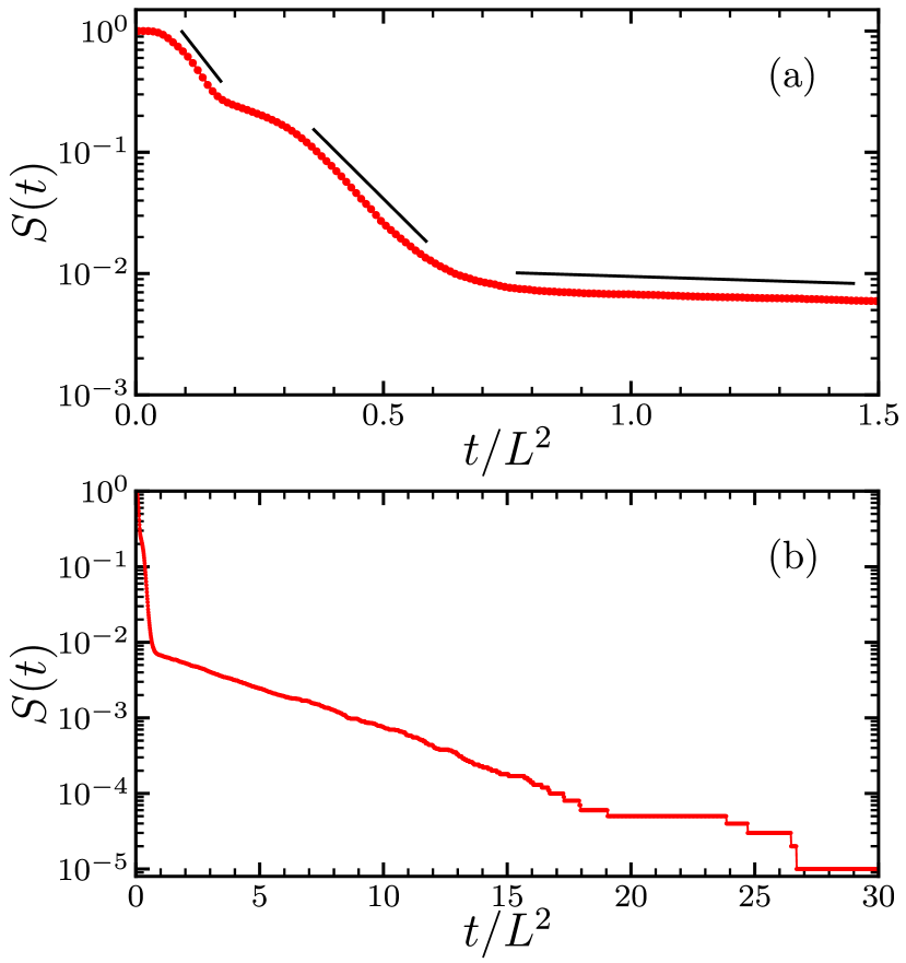
Figure 2: Time dependence of the survival probability $S(t)$ for (a) $t/L^{2}\leq 1.5$ and (b) $t/L^{2}\leq 30$ for a system of linear dimension $L=384$. In (a), the lines schematically indicate the different decay rates associated with coarsening, relaxation to the frozen three-hexagon state, and relaxation to the off-axis three-hexagon/diagonal stripe states.

At short times ($0.05\lesssim t/L\lesssim 0.1$), $S(t)$ decays exponentially in time, with a characteristic decay time that scales as $L^{2}$, corresponding to standard coarsening. This coarsening regime is more readily visible by studying the probability $E(t)$ that the system goes “extinct” at time $t$; this extinction time corresponds to the time when the last flippable spin disappears. This extinction-time distribution is just the negative of the time derivative of the survival probability. As shown in Fig. 3, this distribution has a well-defined short-time peak whose location increases with $L$ as roughly $L^{2}$.

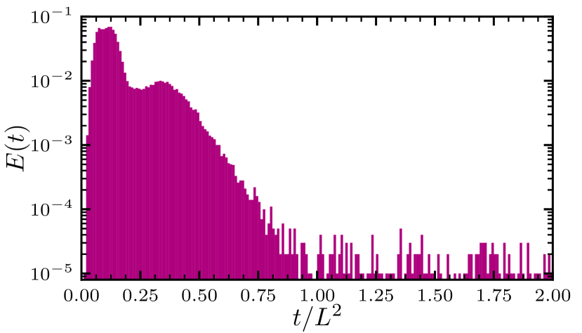
Figure 3: Time dependence of the extinction-time distribution $E(t)$ for a system of linear dimension $L=384$ with $0\leq t/L^{2}\leq 1$.

At long times, defined by $t/L^{2}\gtrsim 0.5$, $S(t)$ decays extremely slowly due to the formation of long-lived diagonal stripe states Spirin et al. (2001a, b) or off-axis three-hexagon states (one such example is given in the $3^{\rm rd}$ panel of Fig. 1(b)). From the asymptote of Fig. 2(a), we roughly estimate the probability for the Potts system to fall into either of these states as $5\times 10^{-3}$ for the largest system that we simulated. When such states form, a large fraction of spins on the diagonal interfaces are in zero-energy environments and thus are freely flippable. As a result, interfaces that are misaligned with the lattice axes are able to diffuse. When two diffusing diagonal interfaces meet, energy-lowering spin flip events occur in which two disjoint spin domains merge. Subsequently, the system quickly falls to the ground state.

For the analogous diagonal stripe states in the kinetic square-lattice Ising ferromagnet, we previously argued that this time to reach the ground state via the diagonal stripe state scales as $L^{\mu}$ with $\mu=3$ (although simulation data indicates that this exponent is closer to 3.5) Spirin et al. (2001a, b). For the Potts ferromagnet, we find that this corresponding relaxation time, $T_{D}$, defined as the time for a system, which enters an off-axis three-hexagon state or a diagonal stripe state, to eventually reach the ground state, again scales as $L^{\mu}$, with $\mu\approx 3.5$ (Fig. 4).

To identify these different time scales, it is helpful to define the reduced moments of the extinction time distribution $M_{n}\equiv\langle t^{n}\rangle^{1/n}$, with the moment itself defined as

$$\langle t^{n}\rangle\equiv\int_{0}^{\infty}dt\,t^{n}E(t)\,.$$ (2)

By construction, $M_{n}$ has the units of time for any $n$ and each $M_{n}$ defines a characteristic time scale of the coarsening process. For large $n$, $M_{n}$ is dominated by the slowest events in $E(t)$ and we identify these with the off-axis three-hexagon/diagonal stripe state relaxation time $T_{D}$. These high-order moments grow as $L^{\mu}$, with $\mu=3.49$ for $M_{8}$ and $\mu=3.50$ for $M_{10}$. Conversely, for small $n$, $M_{n}$ is dominated by the fastest events in $E(t)$, which we identify with the usual coarsening time scale. These low-order moments grow as $L^{\nu}$ with $\nu=2.03$ for $M_{1/10}$ and $\nu=2.06$ for $M_{1/2}$.

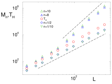
Figure 4: The time scales for the kinetic triangular Potts ferromagnet: (i) $T_{D}$, the off-axis three-hexagon/diagonal stripe relaxation time, which is obtained from $M_{n}$ for large $n$ ($n=8$ and $n=10$ in the plot). (ii) $T_{H}$ ($\circ$), the three-hexagon relaxation time. (iii) The coarsening time, which is obtained from $M_{n}$ for small $n$ ($n=\frac{1}{2}$ and $n=\frac{1}{10}$ in the plot). The dashed lines have slopes 3.5 and 2.

The most interesting dynamics occurs within an intermediate time range defined by $0.2\lesssim t/L^{2}\lesssim 0.5$. Here, $S(t)$ decays with time somewhat more slowly than in the coarsening regime; we argue that this slower time dependence is a manifestation of the spin system reaching a frozen three-hexagon state. We quantify this relaxation by measuring the average time $T_{H}$ for the system to reach this three-hexagon state. As a function of $L$, a naive power-law fit suggests that $T_{H}\sim L^{\eta}$, with $\eta\approx 2.18$. However, there is a consistent, but small, downward curvature in the data of $T_{H}$ versus $L$ on a double logarithmic scale (which becomes visible by magnifying Fig. 4 and/or viewing the data for $T_{H}$ edge on), and a power-law fit is clearly inappropriate.

To help determine the asymptotic behavior of $T_{H}$, we examine the local slopes in the plot of $T_{H}$ versus $L$ that are based on six successive data points of the eleven data points in all (i.e., between points 1–6, points 2–7, $\dots$, points 6–11). These local slopes systematically decrease as the upper limit increases and linearly extrapolate to a value of approximately 2.1. This systematic dependence, as well as an exponent close to an integer value suggests the possibility that $T_{H}$ might be better accounted for by the form $T_{H}\sim L^{2}\ln L$. Indeed, a power-law fit of $T_{H}/\ln L$ versus $L$ gives a much better fit to the data data, albeit with an exponent value of 1.93. However, the data the local exponent based on successive 6-point slopes now shows a very small upward curvature which suggests a larger asymptotic exponent value. Linear extrapolation of the local slopes gives an exponent estimate of 1.95. Based on these numerical results, we are led to the conclusion that $T_{H}\sim L^{2}\ln L$.

This dependence of $T_{H}$ on $L$ appears to have a simple geometrical origin. To reach a frozen three-hexagon state, an initial realization first has to condense to a state that consists of three clusters, none of which span the system (shown in the $3^{\rm rd}$ panel of Fig. 1(a) and schematically on the left side of Fig. 5). This three-cluster state contains geometric distortions whereby the six T-junctions—points where three interfaces meet—are out of registry compared to the aligned T-junctions in the frozen three-hexagon state ($4^{\rm th}$ panel of Fig. 1(a)). Each of the interfaces between pairs of adjacent T-junctions is thus tilted with respect to a triangular lattice direction. This means that a substantial fraction of the spins on each such interface are freely flippable. As indicated in Fig. 6, each freely flippable spin on an interface is equivalent to an independent random walker that can hop along the interface KRB10 .

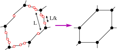
Figure 5: Schematic evolution of the evolution of an off-registry 3-hexagon state to a frozen 3-hexagon state. The red circles indicate freely flippable spins and the heavy dots indicate T-junctions.

The tilted interfaces must gradually straighten for the configuration to reach the frozen three-hexagon state movie . This straightening process occurs by the motion of the equivalent random walkers. When a random walker reaches a T-junction, the position of the latter moves by one lattice spacing. This displacement corresponds to the random walker being absorbed at the T-junction. Thus we can view the process of interface straightening as equivalent to the successive absorption of the order of $L$ independent random walkers on a finite interval whose length is also of the order of $L$.

 

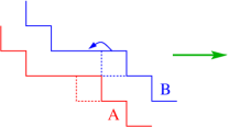
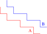
Figure 6: (a) A diagonal stripe interface on the triangular lattice. The $A$ and $B$ spins on corners can flip with no energy cost. (b) The configuration after a spin flip.

When there are $k$ walkers in an interval, their typical separation is $L/k$; this is also the distance between the end of the interval and the closest walker to the interval end. The first-passage time until this closest walker reaches the end of the interval and is absorbed there is given by $t_{k}=\frac{L}{k}\big{(}L-\frac{L}{k}\big{)}$ redner2001guide . When all the walkers along the interfaces have been absorbed, the final, frozen three-hexagon state has been reached. By adding these individual absorption times until all walkers have been absorbed, the time to reach the frozen three-hexagon state is (ignoring constants of order 1),

$$\tau=t_{L}+t_{L-1}+\ldots+t_{1} =\sum_{k=1}^{L}\frac{L}{k}\Big{(}L-\frac{L}{k}\Big{)}$$

$$\simeq L^{2}\ln L\,.$$ (3)

While our argument is crude, it appears to capture the mechanism that underlies the approach to the frozen three-hexagon state. Our prediction is consistent with the simulation results shown in Fig. 4.

IV Final States

A striking aspect of the coarsening of the 3-state triangular Potts ferromagnet is that a new type of final state—a configuration that consists of three hexagons—is reached with a non-zero probability for $L\to\infty$. Figure 7 shows the $L$ dependence of the probabilities for the system to eventually reach: the ground state (probability close to 0.75), a frozen three-hexagon state (probability close to 0.16), a two-stripe state (probability close to 0.09), and three-stripe state (with probability of the order of $10^{-4}$) for the largest system simulated. The three-stripe state plays a negligible role in the coarsening dynamics. Because of the non-monotonic and/or slow $L$ dependences of the final-state probabilities, our estimates for their $L\to\infty$ values are necessarily crude. Similar extrapolation issues were encountered in the kinetic Ising ferromagnet and the square-lattice Potts ferromagnet Spirin et al. (2001a, b); Olejarz et al. (2013).

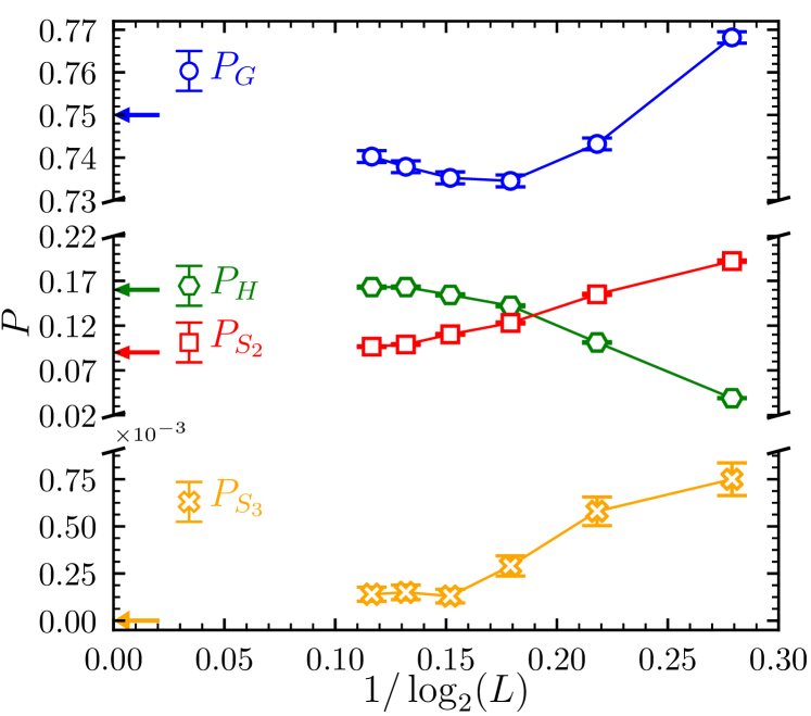
Figure 7: Probabilities of freezing into the ground state, $P_{G}$, a two-stripe state, $P_{S_{2}}$, a frozen three-hexagon state, $P_{H}$, and a three–stripe state $P_{S_{3}}$ as a function of $1/\log_{2}L$. Our $L\to\infty$ estimates of these probabilities are 0.75, 0.09, 0.16, and 0 respectively (arrows).

Intriguingly, the energy of any three-hexagon state (such as the example shown in Fig. 1(a)) equals $24L$, independent of the individual hexagon sizes. By examining the $4^{\rm th}$ panel of Fig. 1(a), the total length of each of the vertical, horizontal, and tilted interfaces in this state must equal $L$. Since there are two spins in different states on either side of the interface, there are $6L$ interfacial spins in total. Because an interfacial spin has four neighbors in the same state and two neighbors in a different state, each such spin contributes $+4J$ to the total energy. Consequently, the final energy of any frozen three-hexagon state is $24L$. Although the total perimeter of the three-hexagon state is fixed, the area of each hexagon is a random quantity whose distribution has a well-defined peak near $\frac{1}{3}$ (Fig. 8). This behavior visually mirrors what was found previously in the kinetic Ising ferromagnet. Here, roughly 1/3 of all realizations condensed into a stripe state, in which the width distribution of the stripes was reasonably fit by a Gaussian distribution  Spirin et al. (2001a, b).

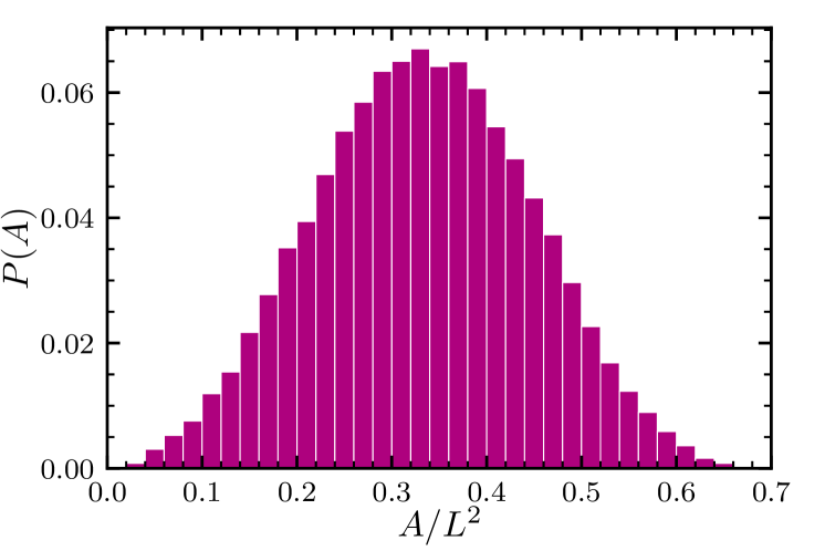
Figure 8: Distribution of the domains areas in the three-hexagon final states for a system of linear dimension $L=384$.

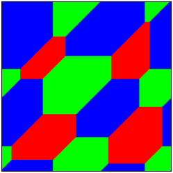
Figure 9: A twelve-hexagon final state in the $q=3$-state Potts ferromagnet. This configuration was found to occur once in $10^{5}$ realizations for a system of linear dimension $L=384$.

Finally, for the 3-state Potts ferromagnet, we also observe static final states that contain more than three hexagons with a vanishingly small probability. Shown in Fig. 9 is an example of a twelve-hexagon state that was observed once in an ensemble of $10^{5}$ realizations for a system of linear dimension $L=384$. Using the same reasoning as that given for the three-hexagon state, it is straightforward to infer that the energy of this twelve-hexagon final state is $48L$. Intriguingly, we did not see, static states that consist of six hexagons in $10^{5}$ realizations. In hindsight, six-hexagon states should not appear because such states cannot be symmetrically situated within a finite-size square domain.

V Potts Ferromagnet with $q>3$ States

Given the rich dynamical behavior of the 3-state Potts ferromagnet, it is natural to investigate this same model with more than three spin states. The dynamics and long-time states of the $q>3$ system shares many features with the 3-state Potts ferromagnet, but additional unusual feature arise. As the number of spin states is increased, the coarsening mosaic becomes visually more picturesque and the possible final states are correspondingly more complex Safran et al. (1982, 1983); Sahni et al. (1983a, b); Grest et al. (1988); Ferrero and Cannas (2007); de Oliveira (2009). Final states that contain more than three hexagons now arise with non-negligible probabilities. To give some examples, for $q=6$ and $L=60$ and 120, we observed five-hexagon states 99 and 106 times, respectively, out of $10^{5}$ realizations (Fig. 10(a)). For $q=20$ and $L=60$ and 120, five-hexagon states were observed 215 and 165 times, respectively, out of $10^{5}$ realizations. We also observed 7 eight-hexagon states out of $10^{5}$ realizations for $q=20$ and $L=60$, but did not observe any such states for L=120 (Fig. 10(b)).

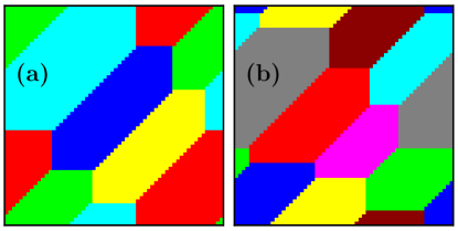
Figure 10: (a) A five-hexagon final state of the $q=6$-state Potts system, and (b) an eight-hexagon state in the $q=20$ Potts system.

Final states that contain blinker spins also exist, but these are extremely rare. We observed blinker spins for $q=5$ and $q=6$ states with a probability of the order of $10^{-4}$, but only for small system sizes. We did not observe blinker spins in any triangular Potts ferromagnet with $L>40$. Both of these exotic long-time states—multi-hexagon states and blinker spins—occur sufficiently rarely that they play a negligible role in characterizing the coarsening dynamics.

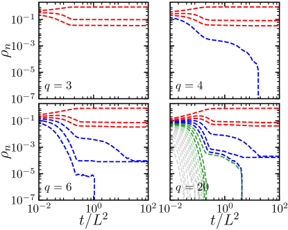
Figure 11: Time evolution of the densities of each spin type, $\rho_{n}$, sorted by abundance order. The data is based on $10^{4}$ realizations on systems of linear dimension $L=240$.

Another intriguing aspect of the large-$q$ Potts ferromagnet is the near universality of the long-time densities of the most-common spin type, the second most-common type, etc., (Fig. 11). Let us denote by $\rho_{1}$, the fraction of the most-common spin type in the final state, $\rho_{2}$, the second most-common spin fraction, etc. Starting with the antiferromagnetic state, with equal numbers of each spin type, the final fractions of the three most abundant spin types are ($\rho_{1},\rho_{2},\rho_{3})\approx(0.870,0.096,0.034)$ for $q=3$ and $(0.893,0.073,0.036)$ for $q=6$ (red in Fig. 11). For $q$ between 3 and 6, the fraction of spins types outside the top three abundances is less than $2\times 10^{-4}$. For $q>6$, the final fractions $\rho_{n}$ for the five most abundant spin types are nearly universal, while the final fractions $\rho_{n}$ for $n>5$ are negligibly small. Thus simulations of Potts ferromagnets with $q>6$ will not reveal new long-time physical features compared to Potts ferromagnets with $q\leq 6$. It is possible there could be final states that contain richer arrangements of hexagons, but these states would play a negligible role in understanding the overall coarsening process.

VI Concluding Remarks

To summarize, the kinetic $q$-state Potts ferromagnet on the triangular lattice exhibits a variety of intriguing topological features. For $q=3$, the final configurations are all static and either: the ground state, frozen three-hexagon states, two-stripe states, or three-stripe states, with respective frequencies of 75%, 9%, 16%, and $<$ 0.02%. Frozen final states that contain more than three hexagons occur with a probability that is less than $10^{-5}$. The dynamics is governed by three distinct time scales: a coarsening time that grows as $L^{2}$, a hexagonal state condensation time $T_{H}$, and an off-axis hexagon/stripe condensation time that grows roughly as $L^{3.5}$. We argued, based on mapping freely flippable spins on hexagonal domain interfaces to a set of independent absorbing random walkers in a finite interval, that $T_{H}\sim L^{2}\ln L$, a prediction that is consistent with simulation data.

We also found that the dynamical behavior of $q>3$-state Potts ferromagnet on the triangular lattice is not materially different than that of the 3-state Potts ferromagnet. For $q>3$ and when the initial state is antiferromagnetic, only the three most abundant spin types are present in measurable amounts at long times. A new feature of the final states for $q>3$ is that frozen configurations that contain more than three hexagons arise. The occurrence probability for these exotic configurations is much larger than in the $q=3$ Potts system, but still only of the order of $10^{-3}$.

There are a variety of open questions raised by this work. First, is it possible to compute the probability to reach the frozen three-hexagon state? The percolation mapping proved decisive to understand the occurrence of various stripe topologies in the kinetic Ising ferromagnet Barros et al. (2009); Olejarz et al. (2012); Blanchard and Picco (2013); Cugliandolo (2016); Blanchard et al. (2017); Yu (2017). Perhaps there is a mapping between final states of the 3-state Potts ferromagnet and the 3-color percolation model, which has only begun to be investigated Z77 ; SY14 . A second open question is to understand the area or the perimeter distribution of the three-hexagon state.

The fact that the final states are simply categorized on the triangular lattice also raises the question of whether there are simple final states for the 3-state Potts ferromagnet on other 6-coordinated lattices, such as the simple cubic lattice. Perhaps there is underlying simplicity when the lattice coordination number is an integer multiple of the number of Potts states. Another unresolved question is the characterization of the final states of the 3-state Potts ferromagnet on the square lattice. While these final states are visually rich and many are apparently non-static Olejarz et al. (2013), they have yet to be quantitatively characterized.

We thank Ben Hourahine and Cris Moore for helpful discussions. JD thanks EPSRC DTA5 grant EP/N509760/1, the Mac Robertson Trust, and the Santa Fe Institute. SR thanks support from NSF grant DMR-1608211. We acknowledge ARCHIE-WeSt High Performance Computer based at the University of Strathclyde as well as grant EP/P015719/1 for computer resources.

References

- Gunton et al. (1982) J. Gunton, M. San Miguel, and P. Sahni, C. Domb and J. L. Lebowitz (Academic, London, 1983) p 267 (1982).
- Bray (2002) A. J. Bray, Adv. Phys. 51, 481 (2002).
- Spirin et al. (2001a) V. Spirin, P. Krapivsky, and S. Redner, Phys. Rev. E 63, 036118 (2001a).
- Spirin et al. (2001b) V. Spirin, P. Krapivsky, and S. Redner, Phys. Rev. E 65, 016119 (2001b).
- Olejarz et al. (2011a) J. Olejarz, P. L. Krapivsky, and S. Redner, Phys. Rev. E 83, 030104 (2011a).
- Olejarz et al. (2011b) J. Olejarz, P. L. Krapivsky, and S. Redner, Phys. Rev. E 83, 051104 (2011b).
- Barros et al. (2009) K. Barros, P. L. Krapivsky, and S. Redner, Phys. Rev. E 80, 040101 (2009).
- Olejarz et al. (2012) J. Olejarz, P. L. Krapivsky, and S. Redner, Phys. Rev. Lett. 109, 195702 (2012).
- Blanchard and Picco (2013) T. Blanchard and M. Picco, Phys. Rev. E 88, 032131 (2013).
- Cugliandolo (2016) L. F. Cugliandolo, J. Stat. Mech. 2016, 114001 (2016).
- Blanchard et al. (2017) T. Blanchard, L. F. Cugliandolo, M. Picco, and A. Tartaglia, J. Stat. Mech. 2017, 113201 (2017).
- Yu (2017) U. Yu, J. Stat. Mech. 2017, 123203 (2017).
- Safran et al. (1982) S. A. Safran, P. S. Sahni, and G. S. Grest, Phys. Rev. B 26, 466 (1982).
- Safran et al. (1983) S. A. Safran, P. S. Sahni, and G. S. Grest, Phys. Rev. B 28, 2693 (1983).
- Sahni et al. (1983a) P. S. Sahni, D. J. Srolovitz, G. S. Grest, M. P. Anderson, and S. A. Safran, Phys. Rev. B 28, 2705 (1983a).
- Sahni et al. (1983b) P. S. Sahni, G. S. Grest, M. P. Anderson, and D. J. Srolovitz, Phys. Rev. Lett. 50, 263 (1983b).
- Grest et al. (1988) G. S. Grest, M. P. Anderson, and D. J. Srolovitz, Phys. Rev. B 38, 4752 (1988).
- Ferrero and Cannas (2007) E. E. Ferrero and S. A. Cannas, Phys. Rev. E 76, 031108 (2007).
- de Oliveira (2009) M. J. de Oliveira, Computer Physics Communications 180, 480 (2009), special issue based on the Conference on Computational Physics 2008.
- (20) M. P. O. Loureiro, J. J. Arenzon, L. F. Cugliandolo, and A. Sicilia, Phys. Rev. E 81, 021129 (2010).
- (21) M. P. O. Loureiro, J. J. Arenzon, and L. F. Cugliandolo, Phys. Rev. E 85, 021135 (2012).
- Glazier et al. (1990) J. A. Glazier, M. P. Anderson, and G. S. Grest, Philos. Mag. B 62, 615 (1990).
- Thomas et al. (2006) G. L. Thomas, R. M. C. de Almeida, and F. Graner, Phys. Rev. E 74, 021407 (2006).
- D.Weaire and Rivier (2009) D.Weaire and N. Rivier, Contemporary Physics 50, 199 (2009).
- Srolovitz et al. (1984) D. Srolovitz, M. Anderson, P. Sahni, and G. Grest, Acta Metallurgica 32, 793 (1984).
- Fradkov and Udler (1994) V. Fradkov and D. Udler, Adv. Phys. 43, 739 (1994).
- Raabe (2000) D. Raabe, Acta Materialia 48, 1617 (2000).
- Zöllner (2011) D. Zöllner, Computational Materials Science 50, 2712 (2011).
- Babcock et al. (1990) K. L. Babcock, R. Seshadri, and R. M. Westervelt, Phys. Rev. A 41, 1952 (1990).
- Jagla (2004) E. A. Jagla, Phys. Rev. E 70, 046204 (2004).
- Mombach et al. (1990) J. C. M. Mombach, M. A. Z. Vasconcellos, and R. M. C. de Almeida, J. Phys. D: Appl. Phys. 23, 600 (1990).
- Mombach et al. (1993) J. C. M. Mombach, R. M. C. de Almeida, and J. R. Iglesias, Phys. Rev. E 48, 598 (1993).
- Hočevar et al. (2010) A. Hočevar, S. El Shawish, and P. Ziherl, Eur. Phys. J. E 33, 369 (2010).
- de Oliveira et al. (2004a) M. J. de Oliveira, A. Petri, and T. Tomé, Physica A: Statistical Mechanics and its Applications 342, 97 (2004a), proceedings of the VIII Latin American Workshop on Nonlinear Phenomena.
- de Oliveira et al. (2004b) M. J. de Oliveira, A. Petri, and T. Tomé, Europhys. Lett. 65, 20 (2004b).
- Olejarz et al. (2013) J. Olejarz, P. L. Krapivsky, and S. Redner, J. Stat. Mech. 2013, P06018 (2013).
- (37) A. B. Bortz, M. H. Kalos, and J. L. Lebowitz, J. Comp. Phys. 17, 10 (1975).
- (38) P. L. Krapivsky, S. Redner, and E. Ben-Naim A Kinetic View of Statistical Physics (Cambridge University Press, Cambridge, UK, 2010) chap. 8.
- (39) See Supplementary Material at https://youtu.be/HwZggJ-7ISo which contains movies showing the relaxation to a static three-hexagon state and to an unstable off-axis three-hexagon state.
- (40) S. Redner, A Guide to First-Passage Processes, (Cambridge University Press, Cambridge, UK, 2001).
- (41) R. Zallen, Phys. Rev. B 16, 1426 (1977).
- (42) S. Sheffield and A. Yadin, Electron. J. Probab. 19, 1 (2014).