Interaction of linear modulated waves and unsteady dispersive hydrodynamic states with application to shallow water waves

Abstract

A new type of wave-mean flow interaction is identified and studied in which a small-amplitude, linear, dispersive modulated wave propagates through an evolving, nonlinear, large-scale fluid state such as an expansion (rarefaction) wave or a dispersive shock wave (undular bore). The Korteweg-de Vries (KdV) equation is considered as a prototypical example of dynamic wavepacket-mean flow interaction. Modulation equations are derived for the coupling between linear wave modulations and a nonlinear mean flow. These equations admit a particular class of solutions that describe the transmission or trapping of a linear wave packet by an unsteady hydrodynamic state. Two adiabatic invariants of motion are identified that determine the transmission, trapping conditions and show that wavepackets incident upon smooth expansion waves or compressive, rapidly oscillating dispersive shock waves exhibit so-called hydrodynamic reciprocity recently described in Maiden et al. (2018) in the context of hydrodynamic soliton tunnelling. The modulation theory results are in excellent agreement with direct numerical simulations of full KdV dynamics. The integrability of the KdV equation is not invoked so these results can be extended to other nonlinear dispersive fluid mechanic models.

1 Introduction

The interaction of waves with a mean flow is a fundamental and longstanding problem of fluid mechanics with numerous applications in geophysical fluids (see e.g. Mei et al. (2005), Bühler (2009) and references therein). Key to the study of such an interaction is scale separation, whereby the length and time scales of the waves are much shorter than those of the mean flow. In the case of small amplitude, linear waves considered here, the induced mean flow is negligible so the effectively external mean flow can be specified separately. See, for example, Peregrine (1976). The linearised dynamical equations exhibit variable coefficients due to the mean flow, mathematically equivalent to the dynamics of linear waves in non-uniform and unsteady media.

Due to the multi-scale character of wave-mean flow interaction, a natural mathematical framework for its description is Whitham modulation theory (Whitham, 1965a, 1999). Although the initial motivation behind modulation theory was the study of finite-amplitude waves, it was recognised that the wave action equation that plays a fundamental role in Whitham theory (Hayes, 1970) was also useful for the study of linearised waves on a mean flow, see e.g. Garrett (1968) and Grimshaw (1984). It was used in Bretherton & Garrett (1968) and Bretherton (1968) to examine the interaction between short-scale, small amplitude internal waves and a mean flow in inhomogeneous, moving media. The outcome of this pioneering work was the determination of the variations of the wavenumber, frequency and amplitude of the linearised wavetrain along group velocity lines. Subsequently, this work was extended in Grimshaw (1975) to finite amplitude waves, incorporating the perturbative effects of friction and compressibility, as well as the leading order effect of rotation.

The modulation theory of linear wavetrains in weakly non-homogeneous and weakly non-stationary media (where weakly is understood as slowly varying in time and/or space) was developed in (Whitham, 1965a; Bretherton & Garrett, 1968). It was shown that the modulation system for the wavenumber $k$, the frequency $\omega$ and the amplitude $a$ is generically composed of the conservation equations

$$k_{t}+\omega_{x}=0\,,\quad\mathcal{A}_{t}+(\partial_{k}\omega\mathcal{A})_{x}=0\,,$$ (1)

where the dispersion relation $\omega(k;\boldsymbol{\alpha}(x,t))$ and the wave action density $\mathcal{A}(a,k;\boldsymbol{\alpha}(x,t))$ depend on the system under study with $\boldsymbol{\alpha}(x,t)$ being a set of slowly varying coefficients describing non-homogeneous non-stationary media that include the effects of the prescribed mean flow, e.g., the current.

Equations (1) were applied to the description of the interaction of water waves with a steady current in (Longuet-Higgins & Stewart, 1961; Peregrine, 1976; Phillips, 1980; Peregrine & Jonsson, 1983; Whitham, 1999; Mei et al., 2005; Bühler, 2009; Gallet & Young, 2014). We briefly outline some classical results from the above references relevant to the developments in this paper. Consider a right-propagating surface wave interacting with a given non-uniform but steady current profile $U(x)$. Assuming slow dependence of $U$ on $x$, the linear dispersion relation reads $\omega=U(x)k+\sigma(k)$ where $\sigma(k)=\sqrt{gk\tanh(kh)}$ is the so-called intrinsic frequency, i.e., the frequency of the wave in the reference frame moving with the current $U$, and $h$ is the unperturbed water depth. The wave action density has the form $\mathcal{A}=\rho ga^{2}/\sigma(k)$. Since $U$ only depends on $x$, we look for a steady solution $k(x)$ and $a(x)$ of the modulation equations (1), which yield: $\omega_{x}=0$ and $(\partial_{k}\omega\mathcal{A})_{x}=0$. Suppose further that $U(x)$ slowly varies between $U_{-}=0$ and $U_{+}$. The wavenumber and the amplitude of the linear wave then slowly changes from some $k_{-},a_{-}$ to $k_{+},a_{+}$, and the conservation of the frequency and the wave action yield the following relations:

$$U_{+}k_{+}+\sigma(k_{+})=\sigma(k_{-})\,,\quad\frac{U_{+}+\partial_{k}\sigma(k_{+})}{\sigma(k_{+})}\,a_{+}^{2}=\frac{\partial_{k}\sigma(k_{-})}{\sigma(k_{-})}\,a_{-}^{2}\,.$$ (2)

There is no analytical solution for Eq. (2) but one can check that $k_{+}$ and $a_{+}$ are decreasing functions of $U_{+}$. The relations (2) have been successfully verified experimentally, cf. for instance (Brevik & Aas, 1980). In particular the linear wave shortens, $k_{+}>k_{-}$, and its amplitude increases, $a_{+}>a_{-}$, when it propagates against the current, $U_{+}<0$. In this case, the group velocity $\partial_{k}\omega(k_{+})=U_{+}+\partial_{k}\sigma(k_{+})$ vanishes for a sufficiently short wave, and no energy can propagate against the current, i.e. the wave is “stopped”, or “blocked” by the current (Taylor, 1955; Lai et al., 1989). Additionally the amplitude of the linear wave $a_{+}$ becomes extremely large and the wave breaks, cf. Eq. (2). As a matter of fact, the linear approximation fails to be valid for such waves. As noted in (Peregrine, 1976), “such a stopping velocity … leads to very rough water surfaces as the wave energy density increases substantially. Upstream of such points, especially if the current slackens, the surface of the water is especially smooth as all short waves are eliminated.” This phenomenon has been observed when the sea draws back at the ebb of the tide where an opposing current increases wave steepness and, as a result, wave breaking occurs (see for instance (Johnson, 1947)). It also enters in some pneumatic and hydraulic breakwater scenarios (cf., (Evans, 1955)) where the injection of a local current destabilises the waves and prevents them from reaching the shore. More recently, wave blocking has been used to engineer the so-called white hole horizon for surface waves in the context of analogue gravity (Rousseaux et al., 2008, 2010). Finally it has been shown that rogue waves can be triggered when surface waves propagate against the current in the ocean (Onorato et al., 2011).

Similar problems for a non-uniform and unsteady mean flow have also been studied. The necessity to consider the media unsteadiness was first recognised by Unna (1941); Barber (1949); Longuet-Higgins & Stewart (1960). Due to the non-stationary character of the problem, the frequency, as well as the wavenumber, are not constant. Various unsteady configurations have been studied with linear theory (1), such as the influence of an unsteady gravity constant on water waves (Irvine, 1985), the effect of internal waves on surface waves (Hughes, 1978), the water wave-tidal wave interaction (Tolman, 1990), and the influence of current standing waves on water waves (Haller & Tuba Özkan-Haller, 2007).

In all described examples, the mean flow or the medium nonhomogeneity were prescribed externally. This results in the simple modulation system (1), consisting of just two equations with variable coefficients, with several implications for the wave’s wavelength and amplitude as outlined above. In this work, we study a different kind of wave-mean flow interaction, where the mean flow dynamically evolves in space-time so that the variations of both the wavetrain and the mean flow are governed by the same nonlinear dispersive PDE but occur in differing amplitude-frequency domains. The dynamics of the small amplitude, short-wavelength wave are dominated by dispersive effects while the large-scale mean flow variation is a nonlinear process. In this scenario, the modulation system (1) for the linear wave couples to an extra nonlinear evolution equation for the mean flow. The form of the mean flow equation depends on the nature of the large-scale unsteady fluid state involved in the interaction. For the simplest case of a smooth expansion (rarefaction) wave, the mean flow equation coincides with the long-wave, dispersionless, limit of the original dispersive PDE. However, if the large-scale, nonlinear state is oscillatory, as happens in a dispersive shock wave (undular bore), the derivation of the mean flow equation requires full nonlinear modulation analysis originally presented in Gurevich & Pitaevskii (1974) (see also El & Hoefer (2016) and references therein). We show that in both cases, the wave-mean flow interaction exhibits two adiabatic invariants of motion that govern the variations of the wavenumber and the amplitude in the linear wavetrain, and prescribe its transmission or trapping inside the hydrodynamic state: either a rarefaction wave (RW) or a dispersive shock wave (DSW). Trapping generalises the aforementioned discussion of blocking phenomena to time-dependent, nonlinear mean flows.

Figure 1: Interaction of a linear wavepacket with nonlinear dispersive hydrodynamic states: a rarefaction wave (left) and a DSW (right)

As a basic prototypical example, we consider dynamic wavepacket-mean flow interactions in the framework of the Korteweg-de Vries (KdV) equation for long shallow water gravity waves:

$$\eta_{t}+c\eta_{x}+\frac{3}{2}\frac{c}{h}\eta\eta_{x}+\frac{h^{2}c}{6}\eta_{xxx}=0\,,$$ (3)

where $h$ is the unperturbed water depth, $\eta(x,t)$ is the free surface elevation relative to $h$ and $c=\sqrt{gh}$ the long-wave speed. Equation (3) exhibits the linear dispersion relation

$$\omega(k,\overline{\eta})=c\left(1+\frac{3\overline{\eta}}{2h}\right)k-\frac{h^{2}c}{6}k^{3}\,,$$ (4)

with frequency $\omega$ and wavenumber $k$. The KdV equation describes uni-directional waves that exhibit a balance between weak nonlinear effects—characterised by the small dimensionless parameter $\eta_{0}/h\ll 1$ where $\eta_{0}$ is the characteristic amplitude of the free surface displacement—and weak dispersive effects—characterised by $k_{0}h\ll 1$ where $1/k_{0}$ is a characteristic horizontal length scale of the perturbation. The balance leading to the KdV equation is

$$\eta_{0}/h\sim(k_{0}h)^{2}\,,$$

Hammack & Segur (1978b). In particular Eq. (3) has proved effective in the quantitative description of surface waves in laboratory experiments (Zabusky & Galvin, 1971; Hammack & Segur, 1974, 1978a; Trillo et al., 2016).

By passing to a reference frame moving at the speed $c$ and normalising $x$ and $\eta$ by the unperturbed depth $h$, and $t$ by the characteristic time $h/c$

$$\tilde{x}=\frac{x-ct}{h},\,\tilde{t}=6\frac{ct}{h},\,u=\frac{9\eta}{h},\,$$ (5)

the KdV equation Eq. (3) assumes its standard form

$$u_{\tilde{t}}+uu_{\tilde{x}}+u_{\tilde{x}\tilde{x}\tilde{x}}=0\,.$$ (6)

In what follows we shall drop tildes for independent variables and shall use the normalised equation (6) as our main mathematical model. All the results obtained in the framework of Eq. (6) can then be readily interpreted in terms of the physical variables using relations (5). The two basic settings we consider for Eq. (6) are illustrated in Fig. 1. The linear wavepacket propagating with group velocity $-3k^{2}$ relative to the background, say $u=u_{0}$, is incident from the right upon an unsteady dispersive-hydrodynamic state: a RW or a DSW. We derive a system of modulation equations describing the coupling between the amplitude-frequency modulations in the linear wave packet and the variations of the background mean flow and show that the linear wave is either transmitted through or trapped inside the unsteady hydrodynamic state. The transmission/trapping conditions are determined by two adiabatic invariants of motion that coincide with Riemann invariants of the modulation system on a certain integral surface.

The mathematical approach to the description of dynamic wave-mean flow interaction that is developed in this paper is general and can be applied to other models for water waves (Lannes, 2013), such as Boussinesq type systems describing bidirectional propagation of nonlinear long waves (Bona et al., 2002, 2004; Serre, 1953), the models for short gravity surface waves (Whitham & Lighthill,, 1967; Trillo et al., 2016), gravity-capillary waves (Schneider & Wayne, 2002), and others.

The paper is organised as follows. In Sec. 2, we introduce the mean field approximation and linear wave theory to derive the modulation system for the interaction of a linear modulated wave with a nonlinear dispersive hydrodynamic state: either a RW or DSW. This system consists of the two usual modulation equations (1) that describe conservation of wave number and wave action, which are coupled to the simple wave evolution equation describing mean flow variations in the RW/DSW. The obtained full modulation system, despite being non-strictly hyperbolic, is shown to possess a Riemann invariant associated with the linear group velocity characteristic. Moreover, we show that the wave action modulation equation can be written in diagonal form, effectively exhibiting an additional Riemann invariant on a certain integral surface.

In Sec. 3, we consider the model problem of plane wave-mean flow interaction whereby the mean flow variations are initiated by Riemann step initial data. Within this framework, the Riemann invariants of the modulation system found in Sec. 2 are shown to play the role of adiabatic invariants of motion that determine the transmission conditions through the RW. The transmission through a DSW is then determined by the same conditions as in the RW case by way of hydrodynamic reciprocity, a notion recently described in the context of soliton-mean flow interactions (Maiden et al., 2018).

The results of Sec. 3 are employed in Sec. 4 to study the physically relevant case of the interaction of localised wavepackets with RWs and DSWs. A partial Riemann problem for wavepacket-RW interaction is used to show that the variation of the wavepacket’s dominant wavenumber is governed by the conservation of the adiabatic invariant identified in Sec. 3 and thus yields the same transmission and trapping conditions for the wave packet as in the full Riemann problem (plane wave-RW interaction). The same conditions are valid, via hydrodynamic reciprocity, for the wavepacket-DSW interaction case. Wavepacket trajectories inside the RW and the DSW are also determined analytically and compared with the results of numerical resolution of the corresponding partial Riemann problem. We obtain the speed and phase shifts of the wavepacket due to its interaction with a hydrodynamic state.

In Sec. 5, we draw conclusions and identify applications and perspectives for further development of this work. Appendix A describes the numerical implementation of the partial Riemann problem employed in Sec. 4.

2 Modulation dynamics of the linear wave-mean flow interaction

2.1 Mean field approximation and the modulation equations

In this section, we shall introduce the mean field approximation that enables a straightforward derivation of the modulation system describing linear wave-mean flow interaction. The full justification of this approximation for the case of the interaction with a RW can be done in the framework of standard multiple-scales analysis (Luke, 1966), equivalent to single-phase modulation theory (Whitham, 1999). The justification for linear wave-DSW interaction is more subtle, requiring the derivation of multiphase (two-phase) nonlinear modulation equations Ablowitz & Benney (1970) and making linearisation in one of the oscillatory phases. To avoid unnecessary technicalities, we simply postulate the approximation used and then justify its validity by comparison of the obtained results with direct numerical simulations of the KdV equation.

To describe the interaction of a linear dispersive wave with an extended nonlinear dispersive-hydrodynamic state (RW or DSW), we represent the solution $u(x,t)$ of the KdV equation (6) as a superposition

$$u(x,t)=u_{\rm H.S.}(x,t)+\varphi(x,t)\,,$$ (7)

where $u_{\rm H.S.}(x,t)$ corresponds to the RW or DSW solution, and $\varphi(x,t)$ corresponds to a small amplitude field describing the linear wave.

In order to extract the dynamics of $\varphi(x,t)$, we make the mean field (scale separation) approximation by assuming that $u_{\rm H.S.}(x,t)$ is locally (i.e. on the scale $\Delta x\sim\Delta t=O(1)$) periodic and replace the dispersive hydrodynamic wave field $u_{\rm H.S.}(x,t)$ with its local mean (period average) value ${\overline{u}}(x,t)$. Within this substitution, the small amplitude approximation and the mean field assumption read

$$\varphi\ll{\overline{u}}\,,\quad{\overline{u}}_{x}/{\overline{u}}\ll\varphi_{x}/\varphi\,,\quad{\overline{u}}_{t}/{\overline{u}}\ll\varphi_{t}/\varphi.$$ (8)

For a smooth, slowly varying hydrodynamic state (RW) such a replacement is natural since locally one has $u_{\rm H.S.}={\overline{u}}$, but for the oscillatory solutions describing slowly modulated nonlinear wavetrains in a DSW, $u_{\rm H.S.}(x,t)\neq{\overline{u}}$ so the mean field approximation would require justification via a careful multiple scale analysis (Ablowitz & Benney, 1970). In particular, a detailed analysis of possible resonances between the DSW and the wavepacket will be necessary (Dobrokhotov & Maslov, 1981). Such a mathematical justification will be the subject of a separate work, while here we shall postulate the outlined mean field approximation and show that it enables a remarkably accurate description of the linear field $\varphi$, which can be thought of as propagating on top of the mean flow.

Within the proposed mean field approximation, the small amplitude wave field $\varphi$ satisfies the linearised, variable coefficient KdV equation

$$\varphi_{t}+{\overline{u}}(x,t)\varphi_{x}+\varphi_{xxx}=0\,,$$ (9)

where the mean flow ${\overline{u}}(x,t)$ evolves according to

$${\overline{u}}_{t}+V({\overline{u}})\,{\overline{u}}_{x}=0\,.$$ (10)

For the case of linear wave-RW interaction: $V({\overline{u}})={\overline{u}}$, and the corresponding simplification of Eq. (10), known as the Hopf equation, is obtained by averaging the KdV equation over linear waves for which $\overline{u^{2}}={\overline{u}}^{2}$ and $\overline{u_{xxx}}=0$ (El, 2005). For the linear wave-DSW interaction, $V({\overline{u}})$ is given parametrically by (Gurevich & Pitaevskii, 1974)

$$\begin{split}&V={\overline{u}}_{+}+\frac{1}{3}({\overline{u}}_{-}-{\overline{u}}_{+})\left(1+m-\frac{2m(1-m)K(m)}{E(m)-(1-m)K(m)}\right)\,,\\ &{\overline{u}}=2{\overline{u}}_{+}-{\overline{u}}_{-}+({\overline{u}}_{-}-{\overline{u}}_{+})\left(m+2\frac{E(m)}{K(m)}\right)\,,\end{split}$$ (11)

where $K(m)$ and $E(m)$ are the complete elliptic integrals of the first and the second kind respectively (Abramowitz & Stegun, 1972), $m\in[0,1]$, and ${\overline{u}}_{-}>{\overline{u}}_{+}$ are the values of $u$ at the left and right constant states respectively, connected by the DSW. The parameter $m$ is implicitly obtained as a self-similar solution with $V=x/t$. Figure 2 displays the variation of the characteristic speed $V({\overline{u}})$ and the mean flow ${\overline{u}}$ for $({\overline{u}}_{-},{\overline{u}}_{+})=(1,0)$. Equations (10), (11) follow from the Whitham modulation system obtained by averaging the KdV equation over the family of nonlinear periodic (cnoidal wave) KdV solutions (Whitham, 1965b). This system consists of three hyperbolic equations that can be diagonalised in Riemann invariant form. The DSW modulation is a simple wave (more specifically, a 2-wave El & Hoefer (2016)) solution of the Whitham equations, in which two of the Riemann invariants are set constant to provide continuous matching with the external constant states $u_{\pm}$ (Gurevich & Pitaevskii, 1974), see also (Kamchatnov, 2000). As we shall show, Eqs. (9), (10), (11) provide an accurate description of the interaction between the linear wave and the DSW so that the dynamics of $\varphi(x,t)$ are predominantly governed by the variations of the DSW mean value ${\overline{u}}(x,t)$.

Figure 2: Left plot: variation of the characteristic speed of the Gurevich-Pitaevskii modulation (11) with $({\overline{u}}_{-},{\overline{u}}_{+})=(1,0)$. Right plot: corresponding variation of the mean flow ${\overline{u}}(x/t)$ inside a DSW. The dashed lines correspond to the DSW edges.

We note that a similar mean flow approach, in which the oscillatory DSW field was replaced by its mean ${\overline{u}}$ has been recently successfully applied to the description of soliton-DSW interaction in Maiden et al. (2018).

Equations (9), (10) form our basic mathematical model for linear wave-mean flow interaction. We shall proceed by constructing modulation equations for this system. One may question the wisdom of incorporating the decoupled mean flow equation (10) to Eq. (9) rather than simply prescribing an arbitrary mean flow externally as has been done in previous works (Bretherton & Garrett, 1968; Bretherton, 1968). As we will see, the mathematical structure of Eqs. (9), (10) enables a convenient solution that is not available for generic mean flows ${\overline{u}}(x,t)$. Moreover, Eqs. (9), (10) transparently reveal the multiscale structure of the dynamics: a fast equation (9) for the linear waves and a slow equation (10) for the mean flow.

Let $\varphi(x,t)$ describe a slowly varying wavepacket:

$$\varphi(x,t)=a(x,t)\cos\left[\theta(x,t)\right]\,,\quad\omega=-\theta_{t}\,,\quad k=\theta_{x}\,,$$ (12)

where

$$a_{x}/a\sim\,k_{x}/k\sim\omega_{x}/\omega\ll k\,,\quad a_{t}/a\sim k_{t}/k\sim\omega_{t}/\omega\ll\omega\,.$$ (13)

These are standard assumptions in modulation theory (Whitham, 1965b, 1999), that can be conveniently formalised by introducing slow space and time variables $X=\varepsilon t$, $T=\varepsilon t$, where $\varepsilon\ll 1$ is a small parameter, and assuming that $a=a(X,T)$, $k=k(X,T)$, $\omega=\omega(X,T)$. To describe the interaction of a linear wave packet with a nonlinear hydrodynamic state, we require that the slow variations of the linear wave’s parameters and the variations of the mean flow occur on the same spatiotemporal scale, i.e. ${\overline{u}}={\overline{u}}(X,T)$. Substituting (12) in (8), we reduce the scale separation conditions between the linear wave and the mean flow to:

$$a\ll{\overline{u}}\,,\quad{\overline{u}}_{x}/{\overline{u}}\ll k\,,\quad{\overline{u}}_{t}/{\overline{u}}\ll\omega\,.$$ (14)

Conditions  (13) and (14) are the main assumptions underlying the modulation theory of linear wave-mean flow interaction described here.

The derivation of modulation equations for $a$ and $k$ is then straightforward using Whitham’s variational approach (cf. for instance (Whitham, 1999), Ch. 11), and yields Eq. (1) with:

$$\omega={\overline{u}}\,k-k^{3},\quad{\cal A}=a^{2}/k\,.$$ (15)

We also derive a useful consequence of the wave conservation law (cf. Eq. (1)) for a wavepacket train consisting of a superposition of two slowly modulated plane waves with close wavenumbers $k$ and $k+\delta k$ where $\delta k\ll k$, which corresponds to beating of the two waves. The conservation of waves for these two waves read

$$k_{t}+\omega(k,{\overline{u}})_{x}=0\,,\quad(k+\delta k)_{t}+\omega(k+\delta k,{\overline{u}})_{x}=0\,.$$ (16)

Hence, for $\delta k\ll k$, the subtraction of these two equations reduces to a conservation equation for $\delta k$ that is very similar to the conservation of wave action:

$$\delta k_{t}+\left(v_{g}(k;{\overline{u}})\delta k\right)_{x}=0\,.$$ (17)

Concluding this section, we note that the modulation system (1), (15) is quite simple and definitively not new. However, unlike in previous studies, it is now coupled to the mean field equation (10). As we shall show, the system consisting of Eqs. (1), (10), (15), and (17) equipped with appropriate initial conditions, yields straightforward yet highly non-trivial implications, especially in the case of wavepacket-DSW interaction, which is very difficult to tackle using direct (non-modulation) analysis.

2.2 Riemann invariants

In what follows, we shall use an abstract field $A(x,t)$ representing either ${\cal A}(x,t)=a(x,t)^{2}/k(x,t)$ or $\delta k(x,t)$ such that the reduced modulation system composed of Eqs. (1), (10), (15), and (17) can be cast in the general form

$${\overline{u}}_{t}+V({\overline{u}}){\overline{u}}_{x}=0\,,$$ (18a)

$$k_{t}+v_{g}(k,{\overline{u}})k_{x}+\partial_{{\overline{u}}}\,\omega(k,{\overline{u}})\,{\overline{u}}_{x}=0\,,$$ (18b)

$$A_{t}+\left(v_{g}(k,{\overline{u}})A\right)_{x}=0\,,$$ (18c)

where $v_{g}(k,{\overline{u}})=\partial_{k}\omega={\overline{u}}-3k^{2}$, $\partial_{{\overline{u}}}\omega=k$, and $V({\overline{u}})={\overline{u}}$ or that given in Eq. (11). We note that the system (18) has the double characteristic velocity $v_{g}$ and thus is not strictly hyperbolic. In fact, there are only two linearly independent characteristic eigenvectors associated with the modulation system (18), so this system of three equations is only weakly hyperbolic. The first two equations, (18a) and (18b), are decoupled and can always be diagonalised such that Eq. (18b) takes the form

$$q_{t}+v_{g}(q,{\overline{u}})q_{x}=0\,,$$ (19)

for the Riemann invariant $q=Q(k,{\overline{u}})$. Generally, the Riemann invariant $q$ as a function of ${\overline{u}}$ and $k$ is found by integrating the characteristic differential form

$$\Xi=[\omega_{k}(k,{\overline{u}})-V({\overline{u}})]dk+\omega_{{\overline{u}}}(k,{\overline{u}})d{\overline{u}}\,.$$ (20)

For the case of linear wave-RW interaction, we have $V({\overline{u}})={\overline{u}}$, so $\Xi=-3k^{2}dk+kd{\overline{u}}$ which can be integrated after multiplying by the integrating factor $1/k$ to yield explicit expressions for the Riemann invariant $q$ and the associated characteristic velocity

$$q=Q(k,{\overline{u}})={\overline{u}}-\frac{3}{2}k^{2}\,,\quad v_{g}(q,{\overline{u}})=2q-{\overline{u}}\,.$$ (21)

It follows from (19) that $q=\hbox{const}\equiv q_{0}$ along the double characteristic $dx/dt=v_{g}$, which enables one to manipulate equation (18c) into the form

$$(pA)_{t}+v_{g}(q_{0},{\overline{u}})(pA)_{x}=0\,,$$ (22)

valid along $dx/dt=v_{g}$, where

$$p=P(q_{0},{\overline{u}})\,,\quad P(q,{\overline{u}})=\exp\left(-\int_{{\overline{u}}_{0}}^{{\overline{u}}}\frac{\partial_{u}v_{g}(q,u)}{V(u)-v_{g}(q,u)}du\right)\,,$$ (23)

with ${\overline{u}}_{0}$ a constant of integration. The quantity $pA$ thus can be viewed as a Riemann invariant of the system (18) on the integral surface $Q(k,{\overline{u}})=q_{0}$ which will prove useful in the analysis that follows. We stress, however, that $pA$ is not a Riemann invariant in the conventional sense since the system (18) does not have a full set of characteristic eigenvectors. See Maiden et al. (2018) for a similar construction in the context of soliton-mean flow interaction.

For $V({\overline{u}})={\overline{u}}$, the integral in (23) is readily evaluated to give, taking into account (21),

$$P(q,{\overline{u}})=\sqrt{\frac{{\overline{u}}-q}{{\overline{u}}_{0}-q}}=\sqrt{\frac{3}{2}}\frac{k}{\sqrt{{\overline{u}}_{0}-q}}\,.$$ (24)

Note, that the described diagonalisation of the reduced modulation system (18) for the linear wave-mean flow interaction, unlike the existence of Riemann invariants of the general Whitham system for modulated cnoidal waves (Whitham, 1965b), does not rely on integrability of the KdV equation. In fact, the possibility of this diagonalisation is general and is a direct consequence of the absence of an induced mean flow for linearised waves, so that the dynamics of the wave parameters $(k,\omega,a)$ are decoupled from the dynamics of the mean flow ${\overline{u}}$. Here, we reap the benefits of jointly considering the evolution of the mean flow, wavenumber conservation, and the field equation in (18) by recognising that they can be cast in diagonal, Riemann invariant form (18a), (19), and (22) along $Q(k,{\overline{u}})=q_{0}$.

3 Plane wave-mean flow interaction: the generalised Riemann problem

3.1 Adiabatic invariants and transmission conditions

Before studying the interaction of localised wavepackets with a mean flow in the framework of the basic system (9), (10), we consider a model problem of the unidirectional scattering of a linear plane wave (PW) by a nonlinear hydrodynamic state (RW or DSW) initiated by a step in ${\overline{u}}$. We denote the incident PW parameters at $x\to+\infty$ as $k_{+},a_{+}$ and the transmitted PW parameters at $x\to-\infty$ as $k_{-},a_{-}$. To find the transmission relations, we consider the generalised Riemann problem (see Fig. 3)

$${\overline{u}}(x,0),\,k(x,0),\,a(x,0)=\begin{cases}{\overline{u}}_{-},k_{-},a_{-}&\text{if }x<0\\ {\overline{u}}_{+},k_{+},a_{+}&\text{if }x>0\end{cases}\,.$$ (25)

We call this Riemann problem generalised as it is formulated for the modulation system (18) rather than for the original dispersive model (9), (10).

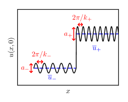
Figure 3: Schematic of the initial conditions for the interaction between a plane wave and a hydrodynamic state.

In the interaction of a PW with both a RW and a DSW, the evolution of ${\overline{u}}(x,t)$ is described by the self-similar expansion fan solution of the mean flow equation (18a):

$${\overline{u}}(x,t)=\begin{cases}{\overline{u}}_{-}&\text{if}\quad x/t<V({\overline{u}}_{-})\\ V^{-1}(x/t)&\text{if}\quad V({\overline{u}}_{-})\leq x/t<V({\overline{u}}_{+})\\ {\overline{u}}_{+}&\text{if}\quad x/t\geq V({\overline{u}}_{+})\end{cases},$$ (26)

while the Riemann invariants $q$ and $pA$ are constant throughout, implying the relations

$$q=Q(k,{\overline{u}})=Q(k_{-},{\overline{u}}_{-})=Q(k_{+},{\overline{u}}_{+})\,,$$ (27)

$$pA=P(k,{\overline{u}})A=P(k_{-},{\overline{u}}_{-})A_{-}=P(k_{+},{\overline{u}}_{+})A_{+}\,,$$ (28)

where $A_{\pm}=a^{2}_{\pm}/k_{\pm}$. These conserved quantities generalise the conservation of wave frequency and wave action, Eq. (2), for steady mean flows to the unsteady case. The expressions for $Q(k,{\overline{u}})$ and $P(k,{\overline{u}})$ in the PW-RW interactions for KdV are given by Eqs. (21) and (24), respectively. For PW-DSW interaction, when $V({\overline{u}})$ is given by Eq. (11), simple explicit expressions for $Q$ and $P$ in terms of $k$ and ${\overline{u}}$ are not available. However, they can be obtained by integrating (20) and evaluating (23), e.g., numerically. The edge speeds of the expansion fan (26) are given by

$$\hbox{RW}:\ \ \qquad V({\overline{u}}_{\pm})={\overline{u}}_{\pm}\,,$$ (29)

$$\hbox{DSW}:\qquad V({\overline{u}}_{-})=2{\overline{u}}_{+}-{\overline{u}}_{-},\quad V({\overline{u}}_{+})=\frac{1}{3}({\overline{u}}_{+}+2{\overline{u}}_{-})\,.$$ (30)

Expressions (30) follow from Eq. (11) upon taking $m\to 0^{+}$ and $m\to 1^{-}$ for the trailing and the leading DSW edge respectively, see Gurevich & Pitaevskii (1974).

Given ${\overline{u}}(x,t)$ described by (26), the conservation of $q$ and $pA$ in (27), (28) yields not only the PW transmission relations but also the slow variations of the PW parameters $k(x/t)$ and $a(x/t)$ due to the interaction with the mean flow in the hydrodynamic state. Constant $q$ and $pA$ can thus be seen as adiabatic invariants of the PW-mean flow interaction.

The conservation relations (27), (28) also describe wave-mean flow interaction for a system of two beating, superposed slowly modulated plane waves with close wavenumbers $k$ and $k+\delta k$ interacting with a RW (cf. Sec. 2.1). In this case, the adiabatic variation of $k$ and $\delta k$ are described respectively by (27) and (28) where $A$ corresponds now to $\delta k$.

As we already mentioned, relations (26), (27) and (28) are valid for both PW-RW (${\overline{u}}_{-}<{\overline{u}}_{+}$) and PW-DSW (${\overline{u}}_{-}>{\overline{u}}_{+}$) interactions. We now consider these two cases in more detail.

3.2 Plane wave-rarefaction wave interaction

A RW is generated when ${\overline{u}}_{-}<{\overline{u}}_{+}$, and the resulting mean flow variation is described by Eq. (26) with characteristic velocity $V({\overline{u}})={\overline{u}}$. In this case, explicit expressions for the adiabatic invariants $q$ and $pA$ can be obtained using Eqs. (21) and (24). The conservation relations (27), (28) then yield

$${\overline{u}}_{-}-\frac{3}{2}k^{2}_{-}={\overline{u}}_{+}-\frac{3}{2}k^{2}_{+}\,,$$ (31)

$$a_{-}=a_{+}\,,$$ (32)

where the second condition was obtained by using $A_{\pm}=a_{\pm}^{2}/k_{\pm}$. It is surprising that the interaction of a PW with a non-uniform, unsteady hydrodynamic state does not change the PW amplitude, which is in sharp contrast with the classical case of the interaction of a surface water wave with a counter-propagating steady current where the amplitude varies following the inhomogeneities of the current in Eq. (2). In this latter case, the wave amplitude can become extremely large during the interaction with the mean flow (and hence the wave is no longer described by linear theory) while Eq. (32) describing dynamic wave-mean flow interaction ensures that the PW remains a small-amplitude linear wave regardless of its wavenumber. In particular no wave-breaking occurs during the interaction with a RW.

Fig. 4 displays the comparison between the relation (31) and the wavenumbers obtained in numerical simulations of linear wave-mean flow interaction. In numerical simulations, we employed the more adequate partial Riemann problem defined in Sec. 4.1 for which we will show that the relation (31) remains valid. One can see that Eq. (31) yields the transmission condition: the transmitted PW exists if its wavenumber $k_{-}$ is a real number. This requirement reduces to the following condition for transmission of the incident PW with wavenumber $k_{+}$:

$$k_{+}>k_{c}=\sqrt{\frac{2}{3}|{\overline{u}}_{+}-{\overline{u}}_{-}|}\,.$$ (33)

The case $k_{+}<k_{c}$ will receive further interpretation in Sec. 4 in the context of the interaction of a localised wavepacket with a RW as wave trapping inside the hydrodynamic state.

One can also consider the interaction between two beating superposed PWs and a RW (see the discussion in Sec. 2.1) where the conservation of the adiabatic invariant $p(k,{\overline{u}})A$ with $A=\delta k$ yields:

$$k_{-}\delta k_{-}=k_{+}\delta k_{+}\,.$$ (34)

As was mentioned in the previous section, the beating pattern created by the superposition of two PWs with close wavenumbers ($\delta k\ll k$) can be seen as a wavepacket train of period $L=4\pi/\delta k$. Thus Eq. (34) provides the relation between the wavelength of the incident train $L_{+}$ and the transmitted train $L_{-}$. The difference

$$\Delta_{-}=L_{-}-L_{+}=L_{+}\left(\frac{k_{-}}{k_{+}}-1\right)$$ (35)

can be interpreted as the phase shift between the incident and the transmitted wavepackets. Similarly, one can interpret $L_{\pm}$ as the widths of the wavepackets before and after transmission. Their relation is then given by

$$\frac{k_{-}}{L_{-}}=\frac{k_{+}}{L_{+}}\,.$$ (36)

3.3 Plane wave-DSW interaction: hydrodynamic reciprocity

We now consider the initial condition (25) with ${\overline{u}}_{-}>{\overline{u}}_{+}$ that resolves into a DSW. In this case, the modulation of the mean flow is described by the simple wave equation  (11), (26) and the expressions for the adiabatic invariants $q$ and $pA$ differ from Eqs. (21), (24) obtained for PW-RW interaction. As a result, the conditions (27), (28) for the conservation of $q$ and $pA$ describe a very different adiabatic evolution of the PW parameters inside the dispersive hydrodynamic state. We shall consider this evolution later in Sec. 4.4, while here we describe a very general property of PW interaction with dispersive hydrodynamic states termed hydrodynamic reciprocity, that was initially formulated in Maiden et al. (2018) for mean field interaction of solitons with dispersive hydrodynamic states.

When ${\overline{u}}_{-}>{\overline{u}}_{+}$, we observe that the PW-DSW and PW-RW interactions in the mean flow approximation are described by the solutions of the same Riemann problem considered for the $t>0$ and $t<0$ half-planes, respectively. Then, continuity of the simple wave modulation solution for all $(x,t)$ (illustrated by Fig. 4, left), except at the origin $(x,t)=(0,0)$, implies that the transition relations (31) and (32) derived for the PW-RW interaction ($t<0$) must also hold for $t>0$, i.e., for the PW-DSW interaction. This hydrodynamic reciprocity is verified in Fig. 4, right where we compare the relations between $k_{-}$ and $k_{+}$ obtained numerically for the evolution of PW-RW and PW-DSW interactions in the full KdV equation. The agreement confirms that relation (31), as well as the transmission condition (33), indeed hold for PW interaction with both nonlinear dispersive hydrodynamic states: RW and DSW.

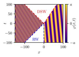
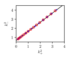
Figure 4: Hydrodynamic reciprocity of plane wave-RW and plane wave-DSW interactions: conservation of $Q(k,{\overline{u}})$ and $a$ in Eqs. (31) and (32). Left plot: modulated plane wave $\varphi=a\cos{\theta}$, $\theta_{x}=k$, $\theta_{t}=-\omega(k,{\overline{u}})$, outside of the domain of interaction with the hydrodynamic state, where ${\overline{u}}_{-}>{\overline{u}}_{+}$, describing PW-DSW interaction for $t>0$ and PW-RW interaction for $t<0$. Right plot: the relationship between the dominant wavenumbers of incident and transmitted wavepackets with $a_{0}=0.01$. The solid line corresponds to the analytical relation (31) when $({\overline{u}}_{-},{\overline{u}}_{+})=(1,0)$. The crosses () and circles () are identified with PW-RW and PW-DSW interaction, respectively. The relation between $k_{-}$ and $k_{+}$ is independent of the nature of the hydrodynamic state.

The agreement between relation (31) and the numerical solution of the Riemann problem in Fig. 4 also confirms the mean field hypothesis underlying the basic mathematical model (9) of this paper. Although the mean field assumption is arguably intuitive for PW-RW interaction where the hydrodynamic state solution $u_{\rm H.S.}$, up to small dispersive corrections at the RW corners, coincides with the solution of (10) for mean flow evolution ${\overline{u}}=V({\overline{u}})$, it is no longer so for the highly nontrivial PW-DSW interaction where $u_{\rm H.S.}$ describes a rapidly oscillating structure, which is radically different from its slowly varying mean flow ${\overline{u}}$ satisfying the equations (10), (11).

The relative difference between the numerically observed wavenumber $k_{-}^{\rm num}$ and the predicted wavenumber $k_{-}$ for transmitted wavepackets through RWs and DSWs is shown in Fig. 5. While the relative error in the small amplitude regime reported in Fig. 4 is on the order of $10^{-3}$, it is surprising that the wavenumber prediction from linear theory holds equally as well for wavepackets with order one amplitudes.

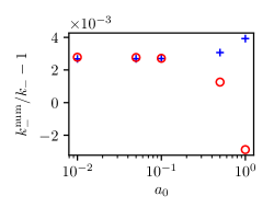
Figure 5: Relative error $k_{-}^{\rm num}/k_{-}-1$ where $k_{-}^{\rm num}$ is obtained numerically and $k_{-}$ satisfies (31) with $k_{+}=0.88$ and $({\overline{u}}_{-},{\overline{u}}_{+})=(0,1)$ (PW-RW) or $({\overline{u}}_{-},{\overline{u}}_{+})=(1,0)$ (PW-DSW). The numerical results are obtained for different amplitudes $a_{0}$ of the incident wavepacket. The crosses () and circles () correspond to the interaction with a RW and DSW, respectively.

3.4 Nonlinear plane wave-mean flow interaction

It is worth taking a brief detour from our general approach, which is applicable to a broad class of nonlinear, dispersive equations, to focus on the KdV equation itself. The reason for this is that, for waves governed by the KdV equation, we can fully describe nonlinear plane wave interaction utilising Whitham theory. We discover three intriguing facts: 1) an arbitrarily large, transmitted nonlinear plane wave conserves its amplitude when interacting with a mean flow (RW or DSW), 2) the linear plane-wave transmission condition in Eq. (31) accurately describes nonlinear plane-wave transmission, and 3) the induced mean flow due to the nonlinear wave is negligible.

For this, we introduce the KdV-Whitham equations that describe the slow modulations of a nonlinear periodic travelling wave solution of the KdV equation (6) (Whitham, 1965b; El & Hoefer, 2016)

$$\frac{\partial r_{j}}{\partial t}+V_{j}\frac{\partial r_{j}}{\partial x}=0\,,\quad j=1,2,3\,,$$ (37)

where $r_{1}$, $r_{2}$, and $r_{3}$ are the modulation parameters that vary slowly relative to the nonlinear wave’s wavelength $2\pi/k$ and temporal period $2\pi/\omega$. A remarkable feature of the KdV-Whitham equations—owing to KdV’s integrable structure—is that $r_{1}$, $r_{2}$, and $r_{3}$ are all Riemann invariants. The characteristic velocities $V_{j}$ are known, ordered ($V_{1}\leq V_{2}\leq V_{3}$), nonlinear functions of the modulation parameters but we will only require

$$V_{3}=\frac{1}{3}(r_{1}+r_{2}+r_{3})+\frac{2}{3}(r_{3}-r_{1})\frac{(1-m)K(m)}{E(m)}\,,\quad m=\frac{r_{2}-r_{1}}{r_{3}-r_{1}}\,.$$ (38)

Note that $V_{2}$ is given in Eq. (11) (with $r_{1}=0$, $r_{2}=m$, and $r_{3}=1$) and determines the DSW mean flow variation. The relationship between the parameters $r_{j}$ and KdV’s nonlinear periodic travelling wave solution is

$$\varphi(x,t)=r_{1}+r_{2}-r_{3}+2(r_{3}-r_{1})\mathrm{dn}^{2}\left(\frac{K(m)}{\pi}\theta;m\right)\,,$$ (39)

where $\mathrm{dn}$ is a Jacobi elliptic function and $\theta=\theta(x,t)$ is the wave’s phase that satisfies the generalised frequency and wavenumber conditions $\theta_{t}=-\omega$, $\theta_{x}=k$ (cf. Eq. (12)). The nonlinear wave’s amplitude, mean, wavenumber, and frequency are determined by the $r_{j}$ according to

$$\begin{split}a&=2(r_{2}-r_{1})\,,\quad\overline{u}=r_{1}+r_{2}-r_{3}+2(r_{3}-r_{1})\frac{E(m)}{K(m)}\,,\\ k&=\frac{\pi\sqrt{r_{3}-r_{1}}}{\sqrt{6}K(m)}\,,\quad\omega=\frac{k}{3}(r_{1}+r_{2}+r_{3})\,.\end{split}$$ (40)

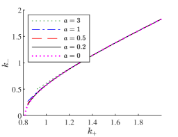
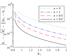
Figure 6: Left plot: transmission relation between the left, $k_{-}$, and right, $k_{+}$, wavenumbers for variable nonlinear plane wave amplitude $a$. Right plot: difference between the finite amplitude wavepacket-mean flow transmission relation $k_{-}(k_{+},a)$ and the zero amplitude relation in Eq. (31). In both plots, the mean flow satisfies $\overline{u}_{-}=0$, $\overline{u}_{+}=1$. Even for large amplitudes, the zero amplitude transmission relation is accurate.

First, we recover the already obtained transmission condition (31) by considering the Riemann problem (25) with $r_{2}\to r_{1}$ so that $a_{\pm}\to 0$ and we are in the linear wave regime. We also have ${\overline{u}}\to r_{3}$ and $k\to 2\sqrt{r_{3}-r_{1}}/\sqrt{6}$. Solving for $r_{1}$, we obtain

$$r_{1}={\overline{u}}-\frac{3}{2}k^{2}\,,$$ (41)

which is precisely the Riemann invariant $q$ in Eq. (21). We also find $V_{3}\to r_{3}$ so that the Riemann invariant $r_{3}={\overline{u}}$ in Eq. (37) ($j=3$) satisfies the mean flow equation (18a) with $V({\overline{u}})={\overline{u}}$ and admits the self-similar solution $r_{3}=x/t$. The other two Riemann invariants coincide and are constant $r_{1}=r_{2}=q$, so that evaluating (41) on the left and right states of the Riemann problem (25) yield the transmission condition (31). The plane wave-RW solution involves variation only in the third characteristic field (Eq. (37) with $j=3$), which is an example of what is termed a 3-wave in hyperbolic systems theory (see, e.g., El & Hoefer (2016)).

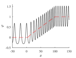
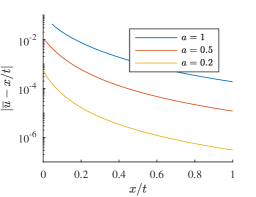
Figure 7: Left plot: asymptotic solution for nonlinear plane wave-RW interaction with $k_{+}=0.85$, ${\overline{u}}_{-}=0$, ${\overline{u}}_{+}=1$, and $a=1$ so that $k_{-}\approx 0.294$ at $t=100$ (solid) and its corresponding mean flow variation (dashed). Right plot: difference between the self-similar RW mean flow variation for $k_{+}=1$ in the 3-wave modulation solution and the zero amplitude result ${\overline{u}}=x/t$. Even for large amplitudes, the zero amplitude mean flow variation is accurate.

We now generalise this result to arbitrary, finite amplitude $a$ by again considering the Riemann problem (25). The 3-wave solution consists of constant Riemann invariants $r_{1}$ and $r_{2}$ with $r_{1}<r_{2}$. Consequently, the nonlinear plane wave amplitude $a=2(r_{2}-r_{1})$, no matter how large, is constant across the self-similar dynamics of the mean flow because it is independent of $r_{3}$. First, we consider a right-incident nonlinear plane wave in which the amplitude $a$, the right wavenumber $k_{+}$, and the left and right mean flows ${\overline{u}}_{-}<{\overline{u}}_{+}$ are given—nonlinear plane wave-RW interaction. Then, the aim is to determine the left wavenumber when a 3-wave solution exists. These four constraints, along with the equations in (40), determine $r_{1}$, $r_{2}$, and $r_{3}^{\mp}$. Then $k_{-}$ is not a free parameter and is determined in terms of the four constraints, which we obtain by numerical solution of the algebraic equations. The absolute difference of the relationship between $k_{-}$ and $k_{+}$ for variable amplitude $a$ and the zero amplitude transmission condition (31) is shown in Fig. 6, left. The error is surprisingly small, even for very large plane wave amplitudes. The self-similar mean flow variation is determined by solving for $r_{3}(x/t)$ when $V_{-}\leq x/t\leq V_{+}$ where $V_{3}(r_{1},r_{2},r_{3})=x/t$ such that $V_{\pm}=V_{3}(r_{1},r_{2},r_{3}^{\pm})$. We perform this calculation numerically and plot the difference between the mean flow variation computed from the zero amplitude result, ${\overline{u}}=x/t$, and the 3-wave solution’s mean flow variation with nonzero amplitude in Fig. 6, right. The influence of the plane wave’s amplitude on the mean flow (i.e. the induced mean flow) is almost negligible, even for very large amplitudes.

The process of obtaining $k_{-}$ in terms of the other flow parameters (${\overline{u}}_{\pm}$, $k_{+}$, and $a$) does not require ${\overline{u}}_{-}<{\overline{u}}_{+}$, therefore the calculation of the transmission relation for nonlinear plane wave-DSW interaction is the same as for nonlinear plane wave-RW interaction and we obtain the same transmission relation. This is yet another explanation of hydrodynamic reciprocity. Note, however, that the mean flow variation will necessarily be different, involving the 2-phase interaction of a DSW with a nonlinear plane wave. We do not study this problem here.

The conservation of the nonlinear plane wave’s amplitude for interactions with RW or DSW mean flows and the accuracy of the zero amplitude transmission relation prediction for nonzero plane wave amplitudes helps explain the numerically observed robustness of our more general small amplitude wavepacket analysis described in the next section.

4 Interaction of linear wavepackets with unsteady hydrodynamic states

4.1 Partial Riemann problem

Having considered the model case of PW interaction with dispersive hydrodynamic states, we now proceed with a more physically relevant example of a similar interaction involving localised linear wavepackets instead of PWs. To model such an interaction, the Riemann problem (18), (25) must be modified to take into account the localised nature of the wavepacket. To this end, we introduce the partial Riemann problem

$$({\overline{u}},k)=\begin{cases}({\overline{u}}_{-},k_{-})&\text{if }x<0\\ ({\overline{u}}_{+},k_{+})&\text{if }x>0\end{cases}\,,\quad a(x,0)=a_{0}f(x-X_{0})\,,$$ (42)

where the amplitude profile is localised and centred at $x=X_{0}$. We take a Gaussian $f(y)=e^{-y^{2}/L_{0}^{2}}$ with width $L_{0}$. In what follows, the position of the wavepacket, defined as a group velocity line, is denoted by $X(t)$, so that according to (42), $X(0)=X_{0}$. While the wavepacket is localised, we consider a sufficiently broad initial amplitude distribution that does not vary significantly over one period $2\pi/k$ of the oscillation of the carrier wave, $L_{0}\gg 2\pi/k_{\pm}$, such that the amplitude modulation is well described by (18c), see conditions (13). We also require $|X_{0}|\gg L_{0}$ so that the initial wavepacket is well-separated from the initial step in the mean flow at the origin.

The quantities $k_{+}$ and $k_{-}$ here denote the dominant wavenumbers of the wavepackets for $x>0$ and $x<0$ respectively. Note that, although the wavepacket dominant wavenumber is defined only along the group velocity line, we treat it here as a spatiotemporal field $k(x,t)$, and the formulation (42) assumes the simultaneous presence of two wavepackets at $t=0$ with dominant wavenumbers $k_{-}$ and $k_{+}$. Still only one of them—we shall call it the incident wavepacket—is physically realised due to the localised nature of the amplitude distribution. The additional, fictitious wavepacket yields all the transmission, trapping information of the incident wavepacket. See Maiden et al. (2018) for a similar extension made to define a soliton amplitude field in the context of the soliton-mean flow interaction problem.

The partial Riemann problem (18), (42) implies two possible interaction scenarios: (i) a right-incident interaction where a wavepacket, initially placed at $X_{0}>0$, propagates with group velocity $v_{g}^{+}={\overline{u}}_{+}-3k_{+}^{2}$ and enters either an expanding hydrodynamic structure whose leading edge velocity is $V({\overline{u}}_{+})>v_{g}^{+}$ (see (29), (30)); (ii) a left-incident interaction, where the wavepacket is initially placed at $X_{0}<0$ so that the interaction only occurs if $V({\overline{u}}_{-})<v_{g}^{-}={\overline{u}}_{-}-3k_{-}^{2}$. It follows from (29), (30) that this can happen only for a DSW but not for a RW.

The subsystem (18a), (18b) and (42) for ${\overline{u}}$ and $k$ has already been solved in the previous section. The simple wave solution of this problem is given by Eqs. (26) and (27), and thus the relation between $k_{-}$ and $k_{+}$ (31) obtained for PWs, holds for the wavepacket-mean flow interaction. As a consequence, the wavepacket is subject to the transmission condition (33). The possible interaction configurations are summarised in Table 1. The partial Riemann problem (6), (42) was solved numerically to verify the relation (31) in Fig. 4. Its numerical implementation is detailed in Appendix A.

Hydro. state	Wavepacket $X_{0}<0$	Wavepacket $X_{0}>0$
RW	$\bullet$ no interaction	$\bullet$ transmitted if: $k_{+}^{2}>2/3({\overline{u}}_{+}-{\overline{u}}_{-})$ $\bullet$ trapped in the RW otherwise
DSW	$\bullet$ no interaction if: $k_{-}^{2}>2/3({\overline{u}}_{-}-{\overline{u}}_{+})$ $\bullet$ trapped in the DSW otherwise	$\bullet$ always transmitted

Table 1: Configuration classification for wavepacket—hydrodynamic state interaction.

4.2 Conservation of the integral of wave action

We now proceed with the determination of the wavepacket amplitude variation resulting from the interaction with dispersive hydrodynamic states. It is well known that KdV dispersion leads to wavepacket broadening so that the amplitude $a(x,t)$ decreases during propagation on a constant mean flow ${\overline{u}}_{-}$ or ${\overline{u}}_{+}$ in order to conserve the integral $\int^{\infty}_{-\infty}a^{2}dx$, which leads to the standard dispersive decay estimate $a\sim t^{-1/2}$ for $t\gg 1$ (Whitham, 1999). Thus, we cannot expect the amplitude transmission relation (32) derived for PWs to remain valid for localised wavepackets. To address this issue, instead of considering the amplitude of the wave, we consider the integral of wave action

$$E(t)=\int_{X_{1}(t)}^{X_{2}(t)}\frac{a(x,t)^{2}}{k(x,t)}dx\,,$$ (43)

between two group lines $dX_{1,2}/dt=v_{g}(k(x,t),{\overline{u}}(x,t))\big{|}_{x=X_{1,2}(t)}$. It then follows from (1) and (15) that the integral (43) is conserved during linear wavepacket propagation through a hydrodynamic state with varying mean flow ${\overline{u}}(x,t)$ (Whitham, 1965a; Bretherton & Garrett, 1968).

If the incident wavepacket is transmitted and remains localised, we can evaluate the integral (43) before $(t<t_{+})$ and after ($t>t_{-}$) the interaction when the wave is localised at the right or the left of the hydrodynamic state, respectively, and where the wavenumber field is uniform $k(x,t)=k_{+}$ for $t<t_{+}$ or $k(x,t)=k_{-}$ for $t>t_{-}$ where $a(x,t)\neq 0$. Thus, the conservation of the integral of wave action $E(t_{-})=E(t_{+})$ yields

$$\frac{1}{k_{-}}\int_{-\infty}^{+\infty}a(x,t_{-})^{2}dx=\frac{1}{k_{+}}\int_{-\infty}^{+\infty}a(x,t_{+})^{2}dx\,,$$ (44)

where we replace the limits of integration $X_{1}$ and $X_{2}$ by $-\infty$ and $+\infty$ since the wavepacket is localised in space. The relation (44) is valid in both linear wavepacket-RW and -DSW interactions, as illustrated in Fig. 8. Similar to the relation between $k_{-}$ and $k_{+}$ (31), Eq. (44) holds beyond the small amplitude limit of the wavepacket as displayed by the right plot in Fig. 8.

In the case of a broad wavepacket of almost constant amplitude, we have the following approximation:

$$\int_{-\infty}^{+\infty}a(x,t_{\pm})^{2}dx\approx a_{\pm}^{2}L_{\pm}\,,$$ (45)

where $a_{\pm}$ and $L_{\pm}$ are, respectively, the constant amplitude and width of the wavepacket before and after interaction with a hydrodynamic state. It follows from the wave conservation law that the widths $L_{\pm}$ of the wavepackets on both sides of the hydrodynamic state satisfy $L_{-}/k_{-}=L_{+}/k_{+}$ (see Eq. (36)) so that Eqs. (44) and (45) yield the approximate conservation of amplitude: $a_{-}\approx a_{+}$, which agrees with Eq. (32) obtained for the limiting case of PW-mean flow interaction.

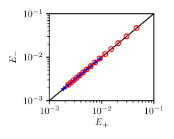
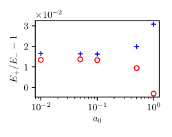
Figure 8: Left plot: comparison between the integral of wave action computed before ($t=t_{+}$), and after ($t=t_{-}$), the transmission of the wavepacket: $E_{\pm}=(\int_{-\infty}^{+\infty}a(x,t_{\pm})^{2}dx)/k_{\pm}$ for the Riemann problem depicted in Fig. 4. The solid line () corresponds to (44) and the crosses () or circles () are obtained numerically from linear wavepacket-RW or -DSW interaction, respectively with $a_{0}=0.01$ and variable $k_{+}$. Right plot: relative error $E_{-}/E_{+}-1$ for $k_{+}=0.88$ and different amplitudes $a_{0}$ of the initial wavepacket.

4.3 Wavepacket-rarefaction wave interaction

In this section, we consider in detail the interaction between a wavepacket and a RW; as we already mentioned, the linear wavepacket interacts with the RW only if initially $x=X_{0}>0$ (see Tab. 1). The fields ${\overline{u}}$ and $k$ are the solution of the Riemann problem studied in Sec. 3.2. The variation of ${\overline{u}}(x,t)$ is described by the relation (26) with $V({\overline{u}})={\overline{u}}$, and the variation of $k(x,t)$ is given by:

$$k(x,t)=\sqrt{k_{+}^{2}-2/3({\overline{u}}_{+}-{\overline{u}}(x,t))}\,,$$ (46)

obtained through the conservation of the adiabatic invariant (21). The identification of a dominant wavenumber when the wavepacket propagates inside the hydrodynamic state implies that $k(x,t)$, or similarly ${\overline{u}}(x,t)$, is almost constant across the wavepacket. This latter condition is readily satisfied for sufficiently large $t$ as the RW mean flow satisfies ${\overline{u}}_{x}=1/t$.

Since the wavepacket propagates with the group velocity $v_{g}(k,{\overline{u}})={\overline{u}}-3k^{2}$, its position $X(t)$ satisfies the characteristic equation

$$\frac{dX}{dt}=v_{g}\left(k(X,t),{\overline{u}}(X,t)\right)\,,\quad X(0)=X_{0}>0\,.$$ (47)

The integration of (47) yields

$$X(t)=\begin{cases}v_{g}(k_{+},{\overline{u}}_{+})\,t+X_{0}&\text{for }0\leq t\leq t_{+}\\ ({\overline{u}}_{+}-\tfrac{3}{2}k_{+}^{2})t+X_{0}t_{+}/(2t)&\text{for }t_{+}\leq t\leq t_{-}\\ v_{g}(k_{-},{\overline{u}}_{-})\,t+3k_{-}^{2}t_{-}&\text{for }t_{-}\leq t\end{cases}\,,$$ (48)

where $t_{+}=X_{0}/(3k_{+}^{2})$ and $t_{-}=X_{0}/(3k_{+}k_{-})$. Hence, during the interaction with the RW, the temporal variation of the dominant wavepacket wavenumber $K(t)$ along the group velocity line is given by

$$K(t)=k(X(t),t)=k_{+}t_{+}/t\,.$$ (49)

The wavepacket trajectory described by Eq. (48) is compared with the numerically observed trajectory in Fig. 9 for two different configurations: transmission ($k_{+}>k_{c}$, cf. (33)) and trapping ($k_{+}<k_{c}$). Snapshots of the envelope $a(x,t)$ of the wavepacket field $\varphi(x,t)$ and the absolute value of its Fourier transform $|\tilde{\varphi}(k,t)|$ are presented in Fig. 10. The numerical procedure implemented to extract $\varphi(x,t)$ from the full numerical solution of (6) is explained in Appendix A.

In Fig. 10, the wavepacket shape in Fourier space slightly deviates from Gaussian when it enters the leading RW edge at $t=500$. However, the wavepacket recovers its Gaussian form when it is fully inside the RW and after exiting the RW.

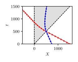
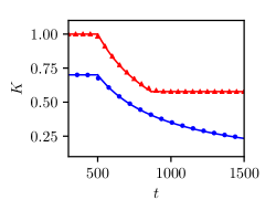
Figure 9: Left plot: trajectories of wavepacket-RW interaction. Solid lines correspond to the solution (48) and markers to the numerical trajectory. The triangles ( ) correspond to the transmission configuration for $k_{+}=1$ and the dots ( ) correspond to the trapping configuration when $k_{+}=0.7$. The RW edges $x={\overline{u}}_{\pm}t$ are represented by dotted lines (). Right plot: the corresponding temporal variation of the wavepacket wavenumber. Solid lines correspond to the solution (49) and markers to the numerical result.

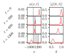
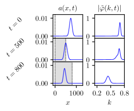
Figure 10: Numerical evolution of wavepacket-RW interaction in the case of transmission (left plot) and trapping (right plot). The first column displays the extracted wavepacket envelope $a(x,t)$. The positions of the RW edges are shown by dotted lines (). The second column displays the amplitude of the wavepacket’s Fourier transform, denoted $\tilde{\varphi}$.

While the wavepacket propagates at constant velocity over a nonmodulated mean flow ${\overline{u}}(x,t)={\overline{u}}_{+}$ or ${\overline{u}}(x,t)={\overline{u}}_{-}$, the wavepacket decelerates during the propagation inside the RW for $t_{+}<t<t_{-}$. Note that acceleration/deceleration here is understood as the increasing/decreasing of the group speed $|v_{g}(X,t)|$. If the transmission condition (33) is not satisfied, $\lim_{t\to\infty}K(t)=0$, and the incident wavepacket gets trapped inside the RW as its velocity $v_{g}={\overline{u}}-3K^{2}$ converges asymptotically to the local background velocity ${\overline{u}}$. Moreover, the wavepacket amplitude decays indefinitely, following the conservation of wave action (43), and the wavepacket eventually gets absorbed by the RW (see Fig. 10, right).

We now draw certain parallels between the trapping of linear waves in RWs and the effect of so-called wave blocking in counter-propagating, inhomogeneous steady currents $U(x)<0$, where the wavenumber $k(x)$ also varies following the inhomogeneities of the current (recall the discussion in Sec. 1). In this case, the adiabatic variation of the wavenumber is simply described by the conservation of the frequency $\omega(k(x);U(x))={\rm const}$. In contrast to wave trapping due to wavepacket-RW interaction considered here, wave blocking in the counter-propagating current is accompanied by a decrease in wavepacket wavelength and an increase in amplitude, until it reaches the stopping velocity $v_{g}=0$ at some finite wavenumber.

The trajectory of the wavepacket displayed in Fig. 9 shows that the wavepacket undergoes refraction due to its interaction with the RW. In the transmission configuration, this results in both a speed shift and a phase shift of the transmitted wavepacket. The phase of the wave after its transmission is equal to $X_{-}=3k_{-}^{2}t_{-}\neq X_{0}$ (cf. Eq. (48) for $t>t_{-}$), so that the phase shift $\Delta_{-}=X_{-}-X_{0}$ is

$$\frac{\Delta_{-}}{X_{0}}=\frac{k_{-}}{k_{+}}-1\,.$$ (50)

This result can also be obtained from the second adiabatic invariant $pA$ in Eq. (28) where $A=\delta k$ as in Eq. (34). Viewing the wavepacket as part of a fictitious periodic train of wavepackets, we recognise that the relative position of the wavepackets post ($x=X_{-}$) and pre ($x=X_{0}$) interaction is inverse to the relative beating wavenumber shift $X_{-}/X_{0}=\delta k_{+}/\delta k_{-}=k_{-}/k_{+}$. Since $k_{-}<k_{+}$, the phase shift is negative in the considered situation. The formula (50) is precisely (35) when we identify $L_{+}$ with $X_{0}$, using the second adiabatic invariant $p\delta k$. Fig. 11 displays the phase shift computed numerically for different wavenumbers $k_{+}$, which agrees with relation (50). In addition, the relation (50) holds for large amplitude wavepackets, just as the relations (31) and (44) do.

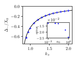
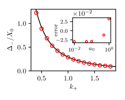
Figure 11: Numerical determination of the normalised phase shift $\Delta_{-}/X_{0}$ for wavepacket-RW interaction (left plot) and wavepacket-DSW interaction (right plot). In the two plots, the markers (pluses  for the RW interaction and circles  for the DSW interaction) correspond to the numerical simulation and the solid line to the analytical prediction (50). The inset plots correspond to the relative error $\Delta_{-}^{\rm num.}/\Delta_{-}-1$ between $\Delta_{-}^{\rm num.}$ determined numerically and $\Delta_{-}$ given by the relation (50). $\Delta_{-}^{\rm num.}$ is obtained for different initial wavepacket amplitudes $a_{0}$, $k_{+}=1.2$ for wavepacket-RW interaction () and $k_{+}=0.88$ for wavepacket-DSW interaction ().

4.4 Wavepacket-DSW interaction

We now consider the more complex case of wavepacket-DSW interaction. Such an interaction is generally described by two-phase KdV modulation theory, which is quite technical, with modulation equations given in terms of hyperelliptic integrals (Flaschka et al., 1980). The mean field approach adopted here enables us to circumvent these technicalities by employing the approximate modulation system (18) that yields simple and transparent analytic results that, as we will show, agree extremely well with direct numerical simulations. More broadly, the notion of hydrodynamic reciprocity described in Sec. 3.3 can be utilised without approximation to make specific predictions for wavepacket-DSW interaction for $t>0$ based on wavepacket-RW interaction for $t<0$.

As already mentioned, wavepacket-DSW interaction admits two basic configurations (see Table 1): the transmission configuration, arising when $X_{0}>0$ and applicable to any incident wavenumber $k_{+}>0$, and the trapping configuration, when $X_{0}<0$ and the incident wavenumber $k_{-}>0$ is sufficiently small. The variation of ${\overline{u}}(x,t)$ inside the DSW is given by ${\overline{u}}=V^{-1}(x/t)$ (see Eq. (26)) where the characteristic velocity $V({\overline{u}})$ is defined by (11).

The variation of the wavepacket’s wavenumber field $k(x,t)$ is given by the adiabatic invariant $q$, which can be obtained by integrating the differential form $\Xi$ in Eq. (20). This differential form vanishes on the group velocity characteristic $dx/dt=v_{g}$, yielding a relation between $k$ and ${\overline{u}}$ specified by the ODE

$$\frac{dk}{d{\overline{u}}}=\frac{\omega_{{\overline{u}}}(k,{\overline{u}})}{V({\overline{u}})-\omega_{k}(k,{\overline{u}})}\,,$$ (51)

with the boundary condition $k({\overline{u}}_{+})=k_{+}$ if $X_{0}>0$ or $k({\overline{u}}_{-})=k_{-}$ if $X_{0}<0$. Note that equation (51) for $V({\overline{u}})={\overline{u}}$ arises in the DSW fitting method where it determines the locus of the KdV DSW harmonic edge, see El (2005); El & Hoefer (2016). Here, it has a different meaning and does not appear to be amenable to analytical solution because of the presence of elliptic integrals in the function $V({\overline{u}})$. We therefore solve (51) numerically. Once the relation $k({\overline{u}})$ has been determined, the $(x,t)$-dependence of the wavenumber inside the DSW is $k=k({\overline{u}}(x,t))=k(V^{-1}(x/t))$. The wavepacket trajectory in the $(x,t)$-plane is obtained by solving (47) with the already determined ${\overline{u}}(x,t)$ and $k(x,t)$. The results of our semi-analytical computations are presented in Figs. 12 and 13.

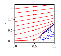
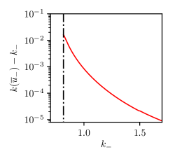
Figure 12: Left plot: wave curves for wavepacket-DSW interaction obtained by numerical integration of Eq. (51) with $({\overline{u}}_{-},{\overline{u}}_{+})=(1,0)$. Solid curves () correspond to transmission configurations ($k({\overline{u}}_{-})>\sqrt{2/3}$), dashed curves () to trapped configurations ($k({\overline{u}}_{-})<\sqrt{2/3}$) and the dash-dotted curve () to the limiting case $k({\overline{u}}_{-})\simeq\sqrt{2/3}$. The arrows correspond to the direction associated with propagation of the wavepacket. Right plot: deviation of the predicted transmitted wavenumber $k(\overline{u}_{-})$ from the actual value $k_{-}$ obtained from Eq. (31) and hydrodynamic reciprocity, as a function of $k_{-}$ with $\overline{u}_{-}=1$, $\overline{u}_{+}=0$. The vertical dash-dotted line is the minimum transmitted wavenumber $k_{-}=\sqrt{2/3}$.

Fig. 12 (left plot) displays the wave curves $k({\overline{u}})$ obtained from the numerical integration of (51), that can be interpreted as wavepacket trajectories in the parameter space $({\overline{u}},k)$. The evolution of the wavepacket’s wavenumber $K(t)=k({\overline{u}}(X/t))$ along a wave curve is then described by an ODE

$$\frac{dK}{dt}=\frac{-K}{V^{\prime}({\overline{u}})t}\,,$$ (52)

obtained by combining ${\overline{u}}=V^{-1}(X/t)$, Eqs. (47) and (51). Since the characteristic speed $V({\overline{u}})$ (10) of the Gurevich-Pitaevskii modulation equation is a decreasing function of ${\overline{u}}$ (cf. Fig. 2), Eq. (52) shows that the wavepacket’s wavenumber is increasing during its propagation inside the DSW, in contrast to wavepacket-RW interaction for which $V^{\prime}({\overline{u}})=1>0$.

We now verify that the obtained integral curves for wavepacket-DSW interaction are consistent with the transmission relation (31) for PW-RW interaction, as required by hydrodynamic reciprocity. In the transmission configuration, where $k({\overline{u}}_{-})>k_{c}=\sqrt{\frac{2}{3}({\overline{u}}_{-}-{\overline{u}}_{+})}$ (see (33)), the wave curve $k({\overline{u}})$ is represented by a solid curve in Fig. 12, left that connects ${\overline{u}}={\overline{u}}_{+}$ to ${\overline{u}}={\overline{u}}_{-}$ and, for a given incident wavenumber $k_{+}$, the transmitted wavenumber is obtained by evaluating $k({\overline{u}}_{-})$. Figure 12, right shows the comparison of the transmitted wavenumber $k({\overline{u}}_{-})$ evaluated by the above semi-analytical procedure with the value $k_{-}=\sqrt{k_{+}^{2}+\frac{2}{3}({\overline{u}}_{-}-{\overline{u}}_{+})}$ obtained from the wavepacket-RW transmission condition Eq. (31) by invoking hydrodynamic reciprocity. The agreement confirms the validity of the mean field approximation and its consistency with hydrodynamic reciprocity.

As expected, the behaviour of wave curves $k({\overline{u}})$ is drastically different for the trapping configuration, when $k({\overline{u}}_{-})<k_{c}$. In this case, the curves $k({\overline{u}})$ (represented by dashed curves in Fig. 12) do not connect ${\overline{u}}={\overline{u}}_{-}$ to ${\overline{u}}={\overline{u}}_{+}$ anymore, implying that the wavepacket initially placed at $x=X_{0}<0$ cannot reach the mean flow ${\overline{u}}={\overline{u}}_{+}$ (trapping). Interestingly, these trapping wave curves $k({\overline{u}})$ are multi-valued, which implies that wavepackets with initial parameters ${\overline{u}}={\overline{u}}_{-},k<k_{c}$ will return, asymptotically as $t\to\infty$, to the DSW harmonic edge where ${\overline{u}}={\overline{u}}_{-}$. More specifically, the point ${\overline{u}}={\overline{u}}_{-},k=k_{c}$ plays the role of an attractor in the parameter space for trapping configurations, such that all the trapped wavepackets’ wavenumbers converge to the same value $k_{c}$ with time. This filtering behaviour is unusual and drastically different from wavepacket-RW trapping (see Sec. 4.3), where the wavepacket trajectory is single-valued and $k\to 0$ as $t\to\infty$.

We now compare the wavepacket dynamics obtained through our modulation analysis with the numerical solution of the KdV equation with initial conditions given by the partial Riemann data (42) (see Appendix A for details of the numerical procedure employed to trace the dynamics of a wavepacket inside a DSW). Fig. 13 displays trajectories for the transmitted and trapped wavepacket configurations, and snapshots of the envelope $a(x,t)$ and the Fourier transform of $\varphi(x,t)$ for the corresponding numerical simulation are presented in Fig. 14. The agreement of the numerical simulations with the analytical predictions in Fig. 13 represents a further confirmation of the mean field approximation employed in the derivation of the basic ODE (51).

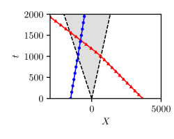
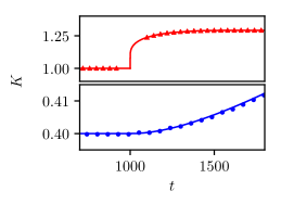
Figure 13: Left plot: trajectories of wavepacket-DSW interaction. Solid lines correspond to semi-analytical solutions obtained by solving (47), (51) and markers to the numerical resolution of the corresponding Riemann problem. The triangles ( ) correspond to the transmission configuration (left propagating wavepacket with $k_{+}=1$) and the dots ( ) correspond to the trapping configuration (right propagating wavepackets with $k_{-}=0.4$). The DSW edge trajectories $x=s_{-}t$ and $x=s_{+}t$ are displayed as dotted lines (): in both cases, we set ${\overline{u}}_{-}=1$ and ${\overline{u}}_{+}=0$. Right plot: corresponding temporal variation of the wavenumbers along the wavepacket trajectories. Solid lines correspond to the semi-analytical solution $K(t)=k({\overline{u}}(X(t),t))$ where $k({\overline{u}})$ has been determined by solving (51) numerically.

Similar to the interaction with a RW, the group velocity of the linear wavepacket is not constant inside the DSW—but now the wavepacket accelerates in the transmission case and simultaneously experiences a wavenumber increase. Here, however, the determination of the wavenumber $K(t)$ is not everywhere possible in the numerical simulation, see Fig. 13. This becomes obvious when one follows the evolution of the amplitude of the Fourier transform $|\tilde{\varphi}(k,t)|$ of the linear field $\varphi(x,t)$ along with the envelope $a(x,t)$ of the field itself (cf. Fig. 14). Initially in our simulations, both distributions have a Gaussian shape, but the Fourier transform of the amplitude distribution loses its unimodality when the wavepacket initially interacts with the leading, soliton, edge of the DSW (see Fig. 14, left plot at $t=1000$). In fact, close to the soliton edge the mean flow gradient ${\overline{u}}_{x}$ is logarithmically singular (Gurevich & Pitaevskii, 1974; El, 2005), see Fig. 2, and the wavenumber field $k(x,t)$ varies significantly over the extent of the wavepacket. As a result, we are no longer in a position to define a nearly monochromatic carrier wave in the wavepacket. Figure 14 shows that the quasi-monochromatic wavepacket structure is recovered when the interaction with the DSW edge is over. Its wavenumber is still described by the adiabatic analytical result while the wavepacket propagates in the region where ${\overline{u}}$ is almost constant over the wavepacket extension. Ultimately $K=k_{-}$, where $k_{-}$ is given by the relation (31), when the wavepacket is no longer interacting with the DSW due to hydrodynamic reciprocity.

The above described logarithmic divergence of the mean field gradient is absent in wavepacket-RW interactions considered in the previous section, where ${\overline{u}}=x/t$ inside the hydrodynamic state such that $k_{x}\propto{\overline{u}}_{x}$ remains finite but exhibits a discontinuity. We still observe a similar, slight deviation from monochromaticity in wavepacket-RW interaction at the initial stage, cf. Fig. 10 $t=500$, with ${\overline{u}}$ varying significantly along the extension of the wavepacket. This behaviour, expectedly, does not appear in the wavepacket-DSW trapping interaction (see Fig. 14, right panel), where the wavepacket, coming from the left of the hydrodynamic state, only interacts with the slowly varying part of the mean flow.

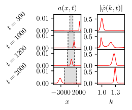
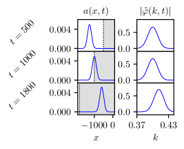
Figure 14: Numerical evolution of wavepacket-DSW interaction, in the transmitted configuration (left plot) and in the trapped configuration (right plot). The first column displays the wavepacket’s envelope amplitude $a(x,t)$ and the positions of the RW edges are indicated by dotted lines (). The second column displays the amplitude of the wavepacket’s Fourier transform.

Similar to wavepacket-RW interaction, we consider the phase shift of the wavepacket transmitted through the DSW. The numerical results are presented in Fig. 11 (right plot, lower panel) and are in agreement with the value predicted analytically in Eq. (50) via hydrodynamic reciprocity.

We note in conclusion that the trapping configuration is somewhat more difficult to treat analytically using the mean field approach employed in other cases. Although the trajectory, as well as the dominant wavenumber of the wavepacket, can be approximately described by our theory for short time evolution (see Fig. 13), we numerically observe that the dynamics of the DSW are no longer decoupled from the dynamics of the linear wave, and the distinction between the two structures becomes less and less pronounced after a sufficiently long time.

5 Conclusions and Outlook

In the context of shallow water theory, we have introduced a general mathematical framework in which to study the interaction of linear wavepackets with unsteady nonlinear dispersive hydrodynamic states: rarefaction waves (RWs) and dispersive shock waves (DSWs) or undular bores. We use a combination of classical Whitham modulation theory and the mean field approximation to derive a new, extended modulation system that describes the dispersive dynamics of a linear wavepacket coupled to the nonlinear, long-wave dynamics of the mean flow in the hydrodynamic state. The mean field equation coincides with the long wave limit of the original dispersive equation when the hydrodynamic state is slowly varying (RW) but has a more complicated structure for rapidly oscillating states (DSWs). We show that the extended modulation system admits a convenient, general diagonalisation procedure that reveals conserved adiabatic invariants during wavepacket evolution through a slowly evolving mean flow. These adiabatic invariants predict transmission relations and trapping conditions for the incident wavepacket. They also imply the hydrodynamic reciprocity property whereby wavepacket interactions with RWs and DSWs exhibit the same transmission/trapping conditions. This enables the circumvention of the complicated analysis of DSW mean field behaviour in order to take advantage of the available wavepacket-RW relations to describe the transmission through a DSW or predict wavepacket trapping inside a DSW. This study has been performed using the KdV equation as a prototypical example, although the integrability properties of the KdV equation were not invoked. The developed theory can be extended to other models supporting multi-scale nonlinear dispersive wave propagation.

While the modulation equations (18) are formally valid only in the limit of vanishingly small amplitude waves, $\varphi\ll\max({\overline{u}})-\min({\overline{u}})$, the numerical simulations demonstrated that the resulting transmission relation (31) between $k_{+}$ and $k_{-}$ also holds for waves of moderate amplitudes $a\sim|{\overline{u}}_{+}-{\overline{u}}_{-}|$. This becomes important for establishing the applicability of the transmission relation (31) to the actual water wave system modelled by the KdV equation for long surface waves in shallow water. In the context of the full water wave model, the KdV equation describes the propagation of weakly nonlinear perturbations to the water surface, so the field $u(x,t)$ already constitutes a small quantity compared to the total depth. Then, considering linearised waves within the KdV approximation would trim the small amplitude limit even further. The robustness of the linear modulation theory results for larger amplitude waves ensures here that the relation (31) remains valid for realistic physical situations where the incident and transmitted waves do not necessarily have small amplitudes within the KdV approximation, but are of the same order $O({\overline{u}}_{+}-{\overline{u}}_{-})$ as the nonlinear hydrodynamic states described by KdV.

The developed modulation theory of linear wave-mean flow interactions could be applied to the interaction of wind-generated short waves with shallow water undular bores in coastal ocean environments. This scenario could readily be tested in wave tank experiments (Hammack & Segur, 1974; Treske, 1994; Frazao & Zech, 2002; Trillo et al., 2016; Rousseaux et al., 2016) where slowly varying mean flows and undular bores have been generated. Another promising application area is to the interaction of small amplitude, short waves with rising and ebbing tide generated mean flows in internal ocean waves. For example, the observed physical parameters pertaining to large-scale undular bores and the Brunt-Väisälä linear dispersion relation in (Scotti, Beardsley, Butman & Pineda, 2008) conform to the assumptions underlying the analysis presented in this paper. The KdV equation can only describe weakly nonlinear internal waves (Helfrich & Melville, 2006). Nevertheless, the theory developed here can readily be generalised to models that capture strongly nonlinear phenomena occurring in a variety of coastal areas (Scotti, Beardsley, Butman & Pineda, 2008; Harris & Decker, 2017; Li, Pawlowicz, & Wang, 2018).

This theory can also be utilised in many physical contexts beyond classical fluid mechanics. In particular, similar to the soliton-mean flow interaction theory very recently developed in Maiden et al. (2018), it can be applied to a broad range of dispersive hydrodynamic systems describing wave propagation in nonlinear optics and condensed matter physics, opening perspectives for experimental observation of the various interaction scenarios studied here. In fact, the linear wavepacket transmission and trapping configurations can be interpreted as hydrodynamic wavepacket scattering, a dispersive wave counterpart of hydrodynamic soliton tunnelling (Maiden et al., 2018; Sprenger et al., 2018). In both cases, the role of a barrier or a scatterer is played by a large-scale, evolving hydrodynamic state that satisfies the same equation as the soliton (wavepacket). Finally, we mention the actively developing field of analogue gravity (see Barceló et al. (2011) and references therein), where the effects of dispersive wave trapping studied here may find interesting interpretations.

A major challenge for the modern theory of dispersive hydrodynamics is to develop a stability theory for dispersive shock waves. The linearisation about a DSW involves a differential operator with both spatially and temporally varying coefficients, presenting significant challenges for its further analysis. The work presented here suggests that perturbations involving sufficiently short wavelengths can be successfully described via wave-mean flow interaction, thus greatly simplifying the stability analysis in this regime.

The developed theory admits generalisations and opens interesting perspectives. It can be extended to physically relevant systems of “KdV type”, such as the asymptotically equivalent, long wave Benjamin-Bona-Mahony equation, the Gardner equation for internal waves, the Kawahara equation for capillary-gravity waves or the viscous fluid conduit equation. Extensions to systems with a nonconvex hyperbolic flux or nonconvex linear dispersion relation may prove fruitful because nonconvexity is known to lead to profound effects in dispersive hydrodynamics: undercompressive and contact DSWs El et al. (2017), expansion shocks (El et al., 2016), DSW implosion (Lowman & Hoefer, 2013) and the existence of resonant and travelling DSWs (Sprenger & Hoefer, 2017). Another natural extension of this work is to the study of linear wave-mean flow interaction in the framework of integrable and non-integrable bidirectional systems such as the defocusing nonlinear Schrödinger equation, the Serre system for fully nonlinear shallow water waves (Serre, 1953), and the Choi-Camassa system for fully nonlinear internal waves Choi & Camassa (1999).

The abstract, basic modulation system (1) has been extensively used in the theory of phase modulations that reveal dispersive deformations arising near coalescing characteristics (see Bridges (2017); Ratliff & Bridges (2016) and references therein). At present, this theory does not include variations of the mean flow. The modulation system that couples modulations of the wavepacket to mean field variations studied here could also be useful for further development of phase modulation theory.

Finally we mention one more area where an appropriate extension of the developed modulation theory could prove useful. It is related to the fundamental problem of mean flow-turbulence interaction (see, e.g., Falkovich (2016) and references therein). A possible connection between weak limits of nonlinear dispersive waves and turbulence theories was conjectured by Lax (1991). Extensions of the modulation theory approach described here to multi-dimensional linear and weakly nonlinear waves provides a plausible entry into this connection.

Appendix A Wavepacket-DSW interaction: numerical resolution

The initial step (42) of the partial Riemann problem is implemented numerically by the function:

$$u(x,t=0)={\overline{u}}_{0}(x)+\varphi_{0}(x)\,,$$ (53)

with:

$$\begin{split}&{\overline{u}}_{0}(x)=\frac{{\overline{u}}_{+}-{\overline{u}}_{-}}{2}\tanh\left(\frac{x}{\xi}\right)+\frac{{\overline{u}}_{+}+{\overline{u}}_{-}}{2}\,,\\ &\varphi_{0}(x)=a_{0}\exp\left(-\frac{(x-X_{0})^{2}}{L_{0}^{2}}\right)\cos\left[k_{\pm}(x-X_{0})\right]\,,\end{split}$$ (54)

where we set $\xi=5$, $L_{0}=120/k_{\pm}$ and, except where otherwise stated, $a_{0}=0.01$. The values for $a_{0}$ and $L_{0}$ are chosen such that $\varphi_{0}$ has small amplitude and is a sufficiently broad wavepacket. The problem (6), (53), (54) is then solved numerically with homogeneous Neumann boundary conditions. The numerical scheme adopted here to solve the KdV equation is explicit, where the space derivatives are approximated using centered finite differences and the time integration is performed with the 4th order Runge-Kutta method. Note that to solve (6), (53), (54) with $({\overline{u}}_{-},{\overline{u}}_{+})=(1,0)$ for $t<0$ in Fig. 4, we solve the equivalent problem with $({\overline{u}}_{-},{\overline{u}}_{+})=(0,1)$ for $t>0$.

In order to determine the variations of the wavepacket $\varphi(x,t)$, we also numerically solve the Riemann problem with the initial condition $u(x,t=0)={\overline{u}}_{0}(x)$ such that we obtain for $t>0$, $u(x,t)=u_{\rm H.S.}(x,t)$. Thus, supposing that the numerical solution $u(x,t)$ of (6), (53), (54) can be put in the form (7), we obtain the variations of the wavepacket $\varphi(x,t)$ by evaluating the difference:

$$\varphi(x,t)=u(x,t)-u_{\rm H.S.}(x,t)\,.$$ (55)

We then extract from the wavepacket amplitude $a(x,t)$, the position of the wavepacket

$$X(t)=\frac{\int_{-\infty}^{+\infty}\,a^{2}(x,t)\,x\,dx}{\int_{-\infty}^{+\infty}a^{2}(x,t)\,dx}\,,$$ (56)

and from the spatial Fourier transform $\tilde{\varphi}(k,t)={\cal F}[\varphi(x,t)]$, the wavepacket dominant wavenumber

$$K(t)=\frac{\int_{-\infty}^{+\infty}|\tilde{\varphi}(k,t)|^{2}\,k\,dk}{\int_{-\infty}^{+\infty}|\tilde{\varphi}(k,t)|^{2}\,dk}\,.$$ (57)

Note that here, the position (56) and the dominant wavenumber (57) correspond to average quantities instead of the pointwise maxima of $a(k,t)$ and $\tilde{\varphi}(k,t)$, respectively, which are not uniquely defined in some situations. When the wavepacket is Gaussian, the quantities (56), (57) are equivalent to the conventional definitions of the wavepacket position and dominant wavenumber.

The ansatz (7) proves to be inadequate to describe the variations of $u(x,t)$ in the trapping interaction with a DSW. We observe that the field $u(x,t)-u_{\rm H.S.}(x,t)$ no longer corresponds to a quasi-monochromatic wavepacket, and exhibits additional small harmonic excitations as in Fig. 15.

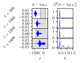
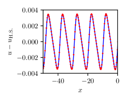
Figure 15: Left plot: numerical evolution of the field $u-u_{\rm H.S.}$ and its spatial Fourier transform wavepacket in the trapping interaction with a DSW. Right plot: the line () corresponds to a zoom in of the oscillation emerging to the right of the wavepacket at $t=1800$. The dots ( ) correspond to the derivative $\partial_{x}u_{\rm H.S.}(x,t)$, rescaled in order to compare with $u-u_{\rm H.S.}$.

We identify this deviation from unimodality as a local phase shift of the DSW. Indeed, it is known that a soliton interacting with a dispersive wavetrain is phase shifted with respect to its free propagation (Ablowitz & Kodama, 1982), and a similar phenomenon could happen for DSWs which are approximately rank-ordered soliton trains. Thus, a schematic solution of the Riemann problem should read:

$$u(x,t)=u_{\rm H.S.}(x-\delta(x,t),t)+\varphi(x,t)\,,$$ (58)

where $\delta(x,t)\ll 1$ corresponds to the small phase-shift induced by the wavepacket-DSW interaction. Yet we determine $\varphi(x,t)$ numerically by computing the difference $u(x,t)-u_{\rm H.S.}(x,t)$ such that

$$u(x,t)-u_{\rm H.S.}(x,t)\approx\varphi(x,t)-\frac{\partial u_{\rm H.S.}(x,t)}{\partial x}\delta(x,t)\,.$$ (59)

The shape of the oscillations of this new linear structure seems to correspond qualitatively to $\partial_{x}u_{\rm H.S.}(x,t)$, cf. Fig. 15.

The evolution of the wavepacket $\varphi$ is recovered numerically by eliminating the term corresponding to the DSW phase shift in (59). This phase-shift contribution can be clearly identified at an early stage of the evolution ($t\sim 10^{-3}$) as the non-adiabatic generation of harmonic excitations in the spatial Fourier transform of $u-u_{\rm H.S.}$. The filtered signal of Fig. 15 is displayed in Fig. 14. It is surprising that, even if the DSW dynamics are slightly perturbed by the wavepacket’s propagation, the wavepacket dynamics are well described by the theory developed here, which confirms, once again, the mean field assumption for wavepacket-DSW interaction.

References

- Ablowitz & Benney (1970) Ablowitz, M. J. & Benney, D. J. 1970 The evolution of multi-phase modes for nonlinear dispersive waves. Stud. Appl. Math. 49, 225–238.
- Ablowitz & Kodama (1982) Ablowitz, M. J. & Kodama, Y. 1982 Note on asymptotic solutions of the Korteweg-de Vries equation with solitons. Stud. Appl. Math. 66, 159–170.
- Abramowitz & Stegun (1972) Abramowitz, M. & Stegun, I. A. 1972 Handbook of mathematical functions with formulas, graphs, and mathematical tables. New York: Dover Publications.
- Barber (1949) Barber, N. F. 1949 The behaviour of waves on tidal streams. Proc. R. Soc. Lon. Ser. A 198 (1052), 81–93.
- Barceló et al. (2011) Barceló, C., Liberati, S., & Visser, M. 2011 Analogue gravity Living Rev. Relativ. 14: 3.
- Bona et al. (2002) Bona, Chen & Saut 2002 Boussinesq equations and other systems for small-amplitude long waves in nonlinear dispersive media. i: derivation and linear theory. J. Nonlinear Sci. 12 (4), 283–318.
- Bona et al. (2004) Bona, J. L., Chen, M. & Saut, J.-C. 2004 Boussinesq equations and other systems for small-amplitude long waves in nonlinear dispersive media: II. The nonlinear theory. Nonlinearity 17 (3), 925–952.
- Bretherton (1968) Bretherton, F. P. 1968 Propagation in slowly varying waveguides. Proc. R. Soc. Lon. Ser. A 302 (1471), 555–576.
- Bretherton & Garrett (1968) Bretherton, F. P. & Garrett, C. J. R. 1968 Wavetrains in inhomogeneous moving media. Proc. R. Soc. Lon. Ser. A 302 (1471), 529–554.
- Brevik & Aas (1980) Brevik, I. & Aas, B. 1980 Flume experiment on waves and currents. I. Rippled bed. Coastal Engineering 3, 149–177.
- Bridges (2017) Bridges, T. J. 2017 Symmetry, phase modulation and nonlinear waves. Cambridge: Cambridge University Press.
- Bühler (2009) Bühler, O. 2009 Waves and mean flows. Cambridge: Cambridge University Press.
- Choi & Camassa (1999) Choi, W. & Camassa, R. 1999 Fully nonlinear internal waves in a two-fluid system. J. Fluid Mech. 396, 1–36.
- Dobrokhotov & Maslov (1981) Dobrokhotov, S. Y. & Maslov, V. P. 1981 Finite-zone, almost-periodic solutions in WKB approximations. J. Math. Sci. 16 (6), 1433–1487.
- El (2005) El, G. A. 2005 Resolution of a shock in hyperbolic systems modified by weak dispersion. Chaos 15, 037103.
- El & Hoefer (2016) El, G. A. & Hoefer, M. A. 2016 Dispersive shock waves and modulation theory. Physica D 333, 11–65.
- El et al. (2016) El, G. A., Hoefer, M. A. & Shearer, M. 2016 Expansion shock waves in regularized shallow-water theory. Proc. R. Soc. Lon. Ser. A 472 (2189), 20160141.
- El et al. (2017) El, G. A., Hoefer, M. A. & Shearer, M. 2017 Dispersive and diffusive-dispersive shock waves for nonconvex conservation laws. SIAM Rev. 59 (1), 3–61.
- Evans (1955) Evans, J. T. 1955 Pneumatic and similar breakwaters. Proc. R. Soc. Lon. Ser. A 231 (1187), 457–466.
- Falkovich (2016) Falkovich, G. 2016 Interaction between mean flow and turbulence in two dimensions. Proc. R. Soc. Lon. Ser. A 472 (2191), 20160287.
- Flaschka et al. (1980) Flaschka, H., Forest, M. G. & McLaughlin, D. W. 1980 Multiphase averaging and the inverse spectral solution of the Korteweg-de Vries equation. Comm. Pure Appl. Math. 33, 739–784.
- Frazao & Zech (2002) Frazao, S. S. & Zech, Y. 2002 Undular bores and secondary waves -Experiments and hybridfinite-volume modelling. J. Hydraul. Res. 40 (1), 33–43.
- Gallet & Young (2014) Gallet, B. & Young, W. R. 2014 Refraction of swell by surface currents J. Mar. Res. 72, 105–126.
- Garrett (1968) Garrett, C. J. R. 1968 On the interaction between internal gravity waves and a shear flow. J. Fluid Mech. 34 (4), 711–720.
- Grimshaw (1975) Grimshaw, R. 1975 Nonlinear internal gravity waves in a rotating fluid. J. Fluid Mech. 71 (3), 497–512.
- Grimshaw (1984) Grimshaw, R. 1984 Wave action and wave-mean flow interaction, with application to stratified shear flows. Annu. Rev. Fluid Mech. 16 (1), 11–44.
- Gurevich & Pitaevskii (1974) Gurevich, A. V. & Pitaevskii, L. P. 1974 Nonstationary structure of a collisionless shock wave. Sov. Phys. JETP 38 (2), 291–297, translation from Russian of A. V. Gurevich and L. P. Pitaevskii, Zh. Eksp. Teor. Fiz. 65, 590-604 (August 1973).
- Haller & Tuba Özkan-Haller (2007) Haller, M. C. & Tuba Özkan-Haller, H. 2007 Waves on unsteady currents. Phys. Fluids 19 (12), 126601.
- Hammack & Segur (1974) Hammack, J. L. & Segur, H. 1974 The Korteweg-de Vries equation and water waves. Part 2. Comparison with experiments. J. Fluid Mech. 65 (2), 289–314.
- Hammack & Segur (1978a) Hammack, J. L. & Segur, H. 1978a The Korteweg-de Vries equation and water waves. Part 3. Oscillatory waves. J. Fluid Mech. 84 (2), 337–358.
- Hammack & Segur (1978b) Hammack, J. L. & Segur, H. 1978b Modelling criteria for long water waves. J. Fluid Mech. 84 (2), 359–373.
- Harris & Decker (2017) Harris, J. C. & Decker, L. 2017 Intermittent large amplitude internal waves observed in Port Susan, Puget Sound. Estuar. Coast. Shelf S. 194, 143–149.
- Hayes (1970) Hayes, W. D. 1970 Conservation of action and modal wave action. Proc. R. Soc. Lon. Ser. A 320 (1541), 187–208.
- Helfrich & Melville (2006) Helfrich, K. R. & Melville, W. K. 2006 Long nonlinear internal waves. Ann. Rev. Fluid Mech. 38, 395–425.
- Hughes (1978) Hughes, B. A. 1978 The effect of internal waves on surface wind waves 2. Theoretical analysis. J. Geophys. Res. C 83 (C1), 455–465.
- Irvine (1985) Irvine, D. E. 1985 The kinematics of short wave modulation by long waves. In The ocean surface: wave breaking, turbulent mixing and radio probing (ed. Y. Toba & H. Mitsuyasu), pp. 129–134. Dordrecht: Springer Netherlands.
- Johnson (1947) Johnson, J. W. 1947 The refraction of surface waves by currents. Eos, Trans. Amer. Geophys. Union 28 (6), 867–874.
- Kamchatnov (2000) Kamchatnov, A. M. 2000 Nonlinear periodic waves and their modulations: an introductory course. Singapore: World Scientific.
- Lai et al. (1989) Lai, R. J., Long, S. R. & Huang, N. E. 1989 Laboratory studies of wave-current interaction: Kinematics of the strong interaction. J. Geophys. Res. C 94 (C11), 16201–16214.
- Lannes (2013) Lannes, D. 2013 The water waves problem. Providence, RI: American Mathematical Society.
- Lax (1991) Lax, P. D. 1991 The zero dispersion limit, a deterministic analogue of turbulence. Comm. Pure Appl. Math. 44 (8–9), 1047–1056.
- Li, Pawlowicz, & Wang (2018) Li, L., Pawlowicz, R. & Wang, C. 2018 Seasonal variability and generation mechanisms of nonlinear internal waves in the strait of Georgia. J. Geophys. Res.-Oceans 123 (8), 5706–5726.
- Longuet-Higgins & Stewart (1960) Longuet-Higgins, M. S. & Stewart, R. W. 1960 Changes in the form of short gravity waves on long waves and tidal currents. J. Fluid Mech. 8 (4), 565–583.
- Longuet-Higgins & Stewart (1961) Longuet-Higgins, M. S. & Stewart, R. W. 1961 The changes in amplitude of short gravity waves on steady non-uniform currents. J. Fluid Mech. 10 (4), 529–549.
- Lowman & Hoefer (2013) Lowman, N. K. & Hoefer, M. A. 2013 Dispersive shock waves in viscously deformable media. J. Fluid Mech. 718, 524–557.
- Luke (1966) Luke, J. C. 1966 A perturbation method for nonlinear dispersive wave problems. Proc. R. Soc. Lon. Ser. A 292 (1430), 403–412.
- Maiden et al. (2018) Maiden, M. D., Anderson, D. V., Franco, N. A., El, G. A. & Hoefer, M. A. 2018 Solitonic dispersive hydrodynamics: theory and observation. Phys. Rev. Lett. 120, 144101.
- Mei et al. (2005) Mei, C. C., Stiassnie, M. & Yue, D. K.-P. 2005 Theory and applications of ocean surface waves. Hackensack, N.J: World Scientific.
- Peregrine (1976) Peregrine, D. H. 1976 Interaction of water waves and currents. Adv. Appl. Mech. 16, 9–117.
- Onorato et al. (2011) Onorato, M., Proment, D. & Toffoli, A. 2011 Triggering rogue waves in opposing currents Phys. Rev. Lett. 107, 184502.
- Peregrine & Jonsson (1983) Peregrine, D. H. & Jonsson, I. G. 1983 Interaction of waves and currents. Tech. Rep. 83-6. CERC, U.S. Army Corps of Engineers.
- Phillips (1980) Phillips, O. M. 1980 The dynamics of the upper ocean. Cambridge; New York: Cambridge University Press.
- Ratliff & Bridges (2016) Ratliff, D. J. & Bridges, T. J. 2016 Whitham modulation equations, coalescing characteristics, and dispersive Boussinesq dynamics. Physica D 333, 107–116.
- Rousseaux et al. (2008) Rousseaux, G., Mathis, C., Maïssa, P., Philbin, T. G. & Leonhardt, U. 2008 Observation of negative-frequency waves in a water tank: a classical analogue to the Hawking effect? New J. Phys. 10 (5), 053015.
- Rousseaux et al. (2010) Rousseaux, G., Maïssa, P., Mathis, C., Coullet, P., Philbin, T. G. & Leonhardt, U. 2010 Horizon effects with surface waves on moving water. New J. Phys. 12 (9), 095018.
- Rousseaux et al. (2016) Rousseaux, G., Mougenot, J.-M., Chatellier, L., David, L., & Calluaud, D. 2016 A novel method to generate tidal-like bores in the laboratory. Euro. J. Mech. B 55, 31–38.
- Schneider & Wayne (2002) Schneider, Guido & Wayne, C. Eugene 2002 The rigorous approximation of long-wavelength capillary-gravity waves. Arch. Rat. Mech. Anal. 162 (3), 247–285.
- Scotti, Beardsley, Butman & Pineda (2008) Scotti, A., Beardsley, R. C., Butman, B & Pineda, J. 2008 Shoaling of nonlinear internal waves in Massachusetts Bay. J. Geophys. Res. 113 (C8), C08031.
- Serre (1953) Serre, F 1953 Contribution à l’ étude des écoulements permanents et variables dans les canaux. La Houille Blanche (3, 6), 374–388, 830–872.
- Sprenger & Hoefer (2017) Sprenger, P. & Hoefer, M. A. 2017 Shock waves in dispersive hydrodynamics with nonconvex dispersion. SIAM J. Appl. Math. 77, 26–50.
- Sprenger et al. (2018) Sprenger, P., Hoefer, M. A. & El, G. A. 2018 Hydrodynamic optical soliton tunneling. Phys. Rev. E 97 (3).
- Taylor (1955) Taylor, G. I. 1955 The action of a surface current used as a breakwater. Proc. R. Soc. Lon. Ser. A 231 (1187), 466–478.
- Tolman (1990) Tolman, H. L. 1990 The influence of unsteady depths and currents of tides on wind-wave propagation in shelf seas. J. Phys. Oceanogr. 20 (8), 1166–1174.
- Treske (1994) Treske, A. 1994 Undular bores (favre-waves) in open channels -Experimental studies. J. Hydraul. Res. 32 (3), 355–370.
- Trillo et al. (2016) Trillo, S., Klein, M., Clauss, G. F. & Onorato, M. 2016 Observation of dispersive shock waves developing from initial depressions in shallow water. Physica D 333, 276–284.
- Unna (1941) Unna, P. J. H. 1941 “White horses”. Nature 148 (3747), 226–227.
- Whitham (1965a) Whitham, G. B. 1965a A general approach to linear and non-linear dispersive waves using a Lagrangian. J. Fluid Mech. 22 (02), 273–283.
- Whitham (1965b) Whitham, G. B. 1965b Non-linear dispersive waves. Proc. R. Soc. Lon. Ser. A 283, 238–261.
- Whitham (1999) Whitham, G. B. 1999 Linear and nonlinear waves. New York, NY: Wiley.
- Whitham & Lighthill, (1967) Whitham, G. B. & Lighthill M. J. 1967 Variational methods and applications to water waves. Proc. R. Soc. Lon. Ser. A 299 (1456), 6–25.
- Zabusky & Galvin (1971) Zabusky, N. J. & Galvin, C. J. 1971 Shallow-water waves, the Korteweg-deVries equation and solitons. J. Fluid Mech. 47 (4), 811–824.