Variational discriminant analysis with variable selection

Abstract

A fast Bayesian method that seamlessly fuses classification and hypothesis testing via discriminant analysis is developed. Building upon the original discriminant analysis classifier, modelling components are added to identify discriminative variables. A combination of cake priors and a novel form of variational Bayes we call reverse collapsed variational Bayes gives rise to variable selection that can be directly posed as a multiple hypothesis testing approach using likelihood ratio statistics. Some theoretical arguments are presented showing that Chernoff-consistency (asymptotically zero type I and type II error) is maintained across all hypotheses. We apply our method on some publicly available genomics datasets and show that our method performs well in practice for its computational cost. An R package VaDA has also been made available on Github.

1 Introduction and literature review

Classification is a fundamental component of machine learning that is applicable in many disciplines. A popular classification method, initially known as discriminant analysis, was first introduced by Fisher (1936) and has more recently been adapted by Dudoit et al. (2002) and Fernández-Delgado et al. (2014) to achieve consistently good performance for some high dimensional datasets. This class of methods involves a comparison of group proportions and group-conditional distributions of variables, also known as features in machine learning literature, to arrive at a classification decision rule. However, this decision rule can not be computed when applying discriminant analysis (DA) to high dimensional data, i.e., when the number of observations, $n$, is less than number of variables, $p$. Furthermore, the standard DA model of Fisher (1936) is not designed to identify discriminative (or signal) variables. Without modification of the base DA model, its usage in high dimensional problems where signal identification is important is limited, e.g., bioinformatics. Moreover, the gradual accumulation of estimation errors as the number of noise variables increases can lead to a substantial loss in classification accuracy (Fan and Fan, 2008).

In discriminant analysis, the group-conditional distribution of variables are commonly assumed to be Gaussian. This simplifies the classification rule to a difference in Mahalanobis distances of a new observation from the group-conditional distributions. Since the MLE of the covariance matrix required to compute the Mahalanobis distance is singular in high dimensional data, i.e., when $n<p$, the classification decision rule cannot be computed. A straightforward solution to this problem is to use alternative estimators such as the Moore-Penrose inverse (Courrieu, 2005; Chen and Feng, 2014; Cai and Liu, 2011) or an alternative covariance matrix. For example, Thomaz et al. (2006) proposed a stabilised covariance matrix, whereas Fisher and Sun (2011) and Guo et al. (2007) used different forms of penalised estimators which we shall describe in further details in Section 6.

Another common solution is to utilise dimension reduction techniques such as principal components or t-distributed stochastic neighbour embeddings (t-SNEs) (van der Maaten and Hinton, 2017) to project the original variables into a lower dimensional space. The high dimensionality issue has also been tackled by making the naïve Bayes assumption, i.e., the covariance matrix for the variables is assumed to be diagonal (Dudoit et al., 2002). Numerous examples of discriminant analysis models, sometimes called naïve Bayes classifiers, that have made this assumption can be found in Tibshirani et al. (2003); Fan and Fan (2008); Witten (2011); Witten and Tibshirani (2011). While dimension reduction solutions are simple to implement, they do not necessarily address the need to identify discriminative variables commonly required in high dimensional data analysis.

An approach that addresses high dimensionality and identifies signal variables is to implement a two-stage algorithm. In the first stage, a hypothesis test is performed on each of the variables to identify signal variables. In the second stage, variables that are identified as signals are retained and used to fit a DA model (e.g., Fan and Fan, 2008). Care must be taken when choosing an appropriate variable selection method as such methods can lead to inflated family-wise type I error, false discovery rates or other multiple testing issues (Shaffer, 1995). This can be easily resolved with one of numerous remedial measures (see for example, Bonferroni, 1936; Benjamini and Hochberg, 1995; Benjamini and Daniel, 2001; Storey, 2003). A notable criterion, known as higher criticism thresholding, exhibits asymptotic optimality and good performance in several multiple testing metrics such as false discovery rate and missed detection rate under some sparsity assumptions (Donoho and Jin, 2004, 2008). This criterion has been incorporated as an option in two-stage DA algorithms such as shrinkage DA (R package: SDA) and factor-adjusted discriminant analysis (R package: FADA) (Ahdesmäki and Strimmer, 2010; Perthame et al., 2016). A modified version of the criterion, known as expanded higher criticism (EHC) (Duarte Silva, 2011), has been incorporated into diagonal linear discriminant analysis (DLDA) and factor-based linear discriminant analysis (R package: HiDimDA). Although many of these algorithms utilise selection criteria that have good theoretical properties, information from the variable selection stage is lost when the variable selection and classification are done in two separate stages. For example, two variables yielding adjusted p-values of $0.001$ and $0.04$ may be selected, but their difference in signal strengths remain unaccounted for. This, in turn, may lead to an unnecessary loss of classification accuracy.

The loss of information can be circumvented by fusing the two stages. This fusion can be realised in penalised discriminant analysis models. In such methods a penalty function induces sparsity in the estimated discriminant vector (product of precision matrix and mean difference), that is used for both variable selection and classification. Witten and Tibshirani (2011) introduced two penalty options to the Fisher’s discriminant problem (R package: penalizedLDA) which will be further elaborated in the Section 6, whereas an $L_{1}$ penalty is introduced through a regression framework in Clemmensen et al. (2011) and Mai et al. (2012). Other examples may be found in Cai and Liu (2011), Shao et al. (2011) and Safo and Ahn (2016). While penalised DA models have demonstrated desirable theoretical properties and good numerical results in these papers, the results are often very sensitive to the setting of the tuning parameter of the penalty function. Usually costly cross-validation is often necessary to determine an appropriate value of this tuning parameter.

In this paper, we propose a Bayesian DA model that integrates both variable selection and classification. The model overcomes high dimensionality by adopting the naïve Bayes assumption leading to an invertible estimated covariance matrix. There are numerous works in the literature that either criticise or justify this assumption. The loss in classification accuracy under this assumption was demonstrated through several simulation studies especially when the correlation structure is complex (Clemmensen, 2013; Perthame et al., 2016) and theoretical criticisms were made in Mai et al. (2012). However, naïve Bayes DA models demonstrated excellent classification performance in several studies on publicly available gene expression datasets (Dudoit et al., 2002; Tibshirani et al., 2003; Fan and Fan, 2008; Witten, 2011) and its worst-case misclassification error has good asymptotic convergence properties under appropriate conditions on the covariance matrix (Bickel and Levina, 2004). The substantially lower computational cost associated with a diagonal covariance matrix also makes the assumption attractive. In our view, the key issue here is a potential trade-off between faster computational speed obtained by using the naïve Bayes assumption and improvement in classification accuracy by accounting for correlation. We believe when there is low to moderate correlation between predictors, or for very high dimensional problems that this trade-off favours naïve Bayes DA.

Unlike the two-stage methods, the Bayesian hierarchical setup of our proposed model fuses both variable selection and classification in an omnibus fashion. By doing so we avoided any loss of information between the variable selection and classification stages. By introducing variable selection parameters into our Bayesian model, we allow posterior inferences to be made on the discriminativeness of each variable. The variable selection component fits naturally into a multiple hypothesis testing (MHT) paradigm. By choosing the cake priors (Ormerod et al., 2017) and approximating the computationally intensive posterior densities with a new variant of variational Bayes inference known as reverse collapsed variational Bayes (RCVB), the resultant decision rule overcomes the problems associated with MHTs such as inflated type I errors. Since the variable selection rule depends on a set of approximate posterior probabilities, the choice of the selection threshold can also be intuitively determined. The resultant classification rule takes the form of a weighted naïve Bayes linear discriminant analysis (when variances are assumed equal). The computational cost of the algorithm is also reduced by utilising Taylor’s approximation to reduce the number of updates in the RCVB cycles. An implementation of our approach uses C++ for high performance computing. These endeavours to keep the computational cost low are aimed at ensuring the scalability of our models to many high dimensional gene expression datasets when computing resources are limited.

In Section 2 we specify the model and discuss our choice of priors. Section 3 introduces our RCVB approximation. We will discuss its application to our model in Section 4. In Section 5, we state some asymptotic properties of our variable selection criterion induced by our proposed model and hence show that our variable selection rule circumvents issues with MHTs. In Section 6 we compare the performance of our proposed model with existing solutions by an application to simulated and publicly available datasets and discuss the choice between two versions of our proposed model. Section 7 concludes.

2 The variational discriminant analysis model

Consider the training dataset $\{{\bf x}_{i},y_{i}\}_{i=1}^{n}$ where for each $i$ we have ${\bf x}_{i}=(x_{i1},\ldots,x_{ip})^{T}$ as a vector of predictor-variables and $y_{i}\in\{0,1\}$ as an observed group label. In this paper, we present the model in the context of a binary classification problem but its extension to multiple groups should be possible. In addition, we have used bold-faced symbols to denote the vector of parameters across subscripts. We assume that $y_{i}$ is observed for all $i=1,\ldots,n$. In line with machine learning terminology, we shall refer to this dataset with observed group labels as the training data.

We consider the following hierarchical model for our data set. For all $i=1,\ldots,n$, each $({\bf x}_{i},y_{i})$ is distributed as follows. Let $\gamma_{j}\in\{0,1\}$, $1\leq j\leq p$ be a binary variable indicating whether variable $j$ is discriminative. If $\gamma_{j}=1$, then

$$\hskip 8.53581pt\left\{\begin{array}[]{ll}x_{ij}\;|\;y_{i},\mu_{j1},\sigma_{j1}^{2}\stackrel{{\scriptstyle\mbox{\scriptsize iid}}}{{\sim}}{\mathcal{N}}(\mu_{j1},\sigma_{j1}^{2})&\mbox{ if $y_{i}=1$; \;}\\[4.30554pt] x_{ij}\;|\;y_{i},\mu_{j0},\sigma_{j1}^{2}\stackrel{{\scriptstyle\mbox{\scriptsize iid}}}{{\sim}}{\mathcal{N}}(\mu_{j0},\sigma_{j1}^{2})&\mbox{ if $y_{i}=0$},\end{array}\right.$$ (1)

and if $\gamma_{j}=0$, then

$$x_{ij}\,|\,\mu_{j},\sigma_{j}^{2}\,\stackrel{{\scriptstyle\mbox{\scriptsize iid}}}{{\sim}}\,{\mathcal{N}}(\mu_{j},\sigma_{j}^{2}),$$ (2)

where ${\mathcal{N}}(m,s^{2})$ denotes the Gaussian distribution with mean $m$ and variance $s^{2}$. When $\gamma_{j}=1$, discriminativeness is induced by imposing dependence between the Gaussian parameters and group label $y_{i}$. We model the conditional distribution of the group labels as

$$y_{i}\,|\,\rho_{y}\,\stackrel{{\scriptstyle\mbox{\scriptsize iid}}}{{\sim}}\,\text{Bernoulli}(\rho_{y}),$$

where $\rho_{y}$ denotes the probability of observing a group 1 sample from the population.

To avoid the computational problem of inverting huge covariance matrices, we make the the naïve Bayes assumption by imposing conditional independence between the variables given the Gaussian parameters and group labels, i.e. $x_{ij}\,\raisebox{0.50003pt}{\rotatebox[origin={c}]{90.0}{$\models$}}\,x_{ik}$ for any $j\neq k$.

2.1 Homogeneity of group-specific variances

We have assumed that the group conditional variances are equal, i.e,. Var$(x_{ij}|y_{i}=1,\sigma_{j1}^{2})=$ Var$(x_{ij}|y_{i}=0,\sigma_{j1}^{2})$. Gaussian discriminant analysis models that adopt this assumption are known as linear discriminant analysis (LDA) since the resultant decision rule is linear in the variables ${\bf x}$ (see Bickel and Levina, 2004; Ahdesmäki and Strimmer, 2010; Duarte Silva, 2011; Witten and Tibshirani, 2011; Clemmensen et al., 2011; Perthame et al., 2016). Those that allow for different group conditional variances are known as quadratic discriminant analysis (QDA) (Srivastava et al., 2007). The choice between LDA and QDA boils down to conditions which LDA is robust to the violation of variance homogeneity. Some simulation studies (Marks and Dunn, 1974; Zavorka and Perrett, 2014) led to the unexpected conclusion that LDA exhibits better performance than QDA when the sample size is small and the departure from the variance homogeneity assumption is mild. As pointed out by a reviewer, this superiority can be understood by observing that LDA has lesser parameters than QDA. Consequently, the more efficient parameter estimation compensates for the model misspecification. In spite of existing findings, superior performance by LDA cannot be guaranteed in publicly available datasets where it is plausible for us to have many true signals with large differences in group-conditional variances. While a compromising solution between QDA and LDA has been proposed by Friedman (1989), we propose two variants of our model - a variational linear discriminant analysis (VLDA) and a variational quadratic discriminant analysis (VQDA), that correspond to LDA and QDA methods respectively. This allows us to study the robustness of naïve Bayes LDA under varying differences in the group-conditional variances and have a QDA version of our proposed model ready when LDA fails.

2.2 Choice of priors

The choice of priors is of paramount importance in Bayesian modelling as it affects the computational course of the posterior inference and allows prior knowledge to influence results of the analysis. A natural choice of priors for ${\boldsymbol{\gamma}}$ and $\rho_{y}$ uses

$$\gamma_{j}\;|\;\rho_{\gamma}\stackrel{{\scriptstyle\mbox{\scriptsize iid}}}{{\sim}}\text{Bernoulli}(\rho_{\gamma}),\quad\mbox{with}\quad\rho_{\gamma}\sim\text{Beta}(a_{\gamma},b_{\gamma}),$$

and

$$\rho_{y}\sim\text{Beta}(a_{y},b_{y}),$$

where the random parameter $\rho_{\gamma}$ may be interpreted as the probability of including a true signal in the dataset.

For the rest of this paper, we have chosen a flat prior for $\rho_{y}$ by assigning the hyperparameters $a_{y}=b_{y}=1$. When considering settings for $a_{\gamma}$ and $b_{\gamma}$, we assume that the true model consists of $p_{0}$ noise and $p_{1}$ signal variables, and that the total number of variables grow at a non-polynomial rate of $n$. Here, we propose the setting $a_{\gamma}=1$ and

$$b_{\gamma}=\frac{p_{n}^{2}}{\sqrt{n+1}}\exp\left[\frac{\kappa(n+1)}{\log(n+1)^{r}}\right]$$ (3)

for some $r<1$ and $\kappa>0$, to induce desirable asymptotic properties in our resultant variable selection rule (see Section 5).

The choice of priors for the Gaussian parameters is a more complex issue. Most research is conducted in the absence of reliable prior knowledge and therefore diffuse priors are a popular choice. However, a diffuse prior may not retain the “diffuse” property after a model reparametrisation. Besides this property, we also require our priors to lead to model selection consistency in our variable selection rule and strong concordance with frequentist approaches (information consistency) in both variable selection and classification rules. The latter criterion would help avoid unnecessary dilemma when users compare the inference results of our model with most other discriminant analysis models that are frequentist in approach.

Recently, Ormerod et al. (2017) has proposed the cake prior which can be made diffuse under some setting of hyperparameters. For a two-sample test of Gaussian data, they have also obtained Bayes factors which have good asymptotic properties. Furthermore, the Bayes factor takes the form of a penalized likelihood ratio statistic. The cake priors for our Gaussian parameters are as follows. For VLDA the model under $H_{0j}$ for variable $j$ is (2) and the model under $H_{1j}$ for variable $j$ is (1). The cake priors for these hypotheses are given by

$$\mu_{j}|\sigma_{j}^{2}\sim{\mathcal{N}}(0,h^{1/2}\sigma_{j}^{2}),\;\;\;\sigma_{j}^{2}\stackrel{{\scriptstyle\mbox{\scriptsize iid}}}{{\sim}}LN(0,2h^{1/2}),$$

$$\mu_{jk}|\sigma_{j1}^{2}\sim{\mathcal{N}}(0,(n/n_{k})h^{1/3}\sigma_{j1}^{2})\;\text{for}\;k=0,1,$$

$$\text{and }\sigma_{j1}^{2}\stackrel{{\scriptstyle\mbox{\scriptsize iid}}}{{\sim}}LN(0,2h^{1/3}).$$

where $n_{1}=\sum_{i=1}^{n}y_{i}$, $n_{0}=n-n_{1}$, $LN$ refers to the log-normal distribution and $h>0$ is a common hyperparameter shared between $\{H_{0j}\}_{j=1}^{p}$ and $\{H_{1j}\}_{j=1}^{p}$.

Analogously, the VQDA model under $H_{1j}$ is

$$\hskip 8.53581pt\left\{\begin{array}[]{ll}x_{ij}\;|\;y_{i},\mu_{j1},\sigma_{j1}^{2}\stackrel{{\scriptstyle\mbox{\scriptsize iid}}}{{\sim}}{\mathcal{N}}(\mu_{j1},\sigma_{j1}^{2})&\mbox{ if $y_{i}=1$; \;}\\[4.30554pt] x_{ij}\;|\;y_{i},\mu_{j0},\sigma_{j0}^{2}\stackrel{{\scriptstyle\mbox{\scriptsize iid}}}{{\sim}}{\mathcal{N}}(\mu_{j0},\sigma_{j0}^{2})&\mbox{ if $y_{i}=0$},\end{array}\right.$$ (4)

and is equivalent to (2) under $H_{0j}$ so that the group conditional variances differ. The cake priors in this case are given by

$$\mu_{j}|\sigma_{j}^{2}\sim{\mathcal{N}}(0,h^{1/2}\sigma_{j}^{2}),\;\;\;\sigma_{j}^{2}\stackrel{{\scriptstyle\mbox{\scriptsize iid}}}{{\sim}}LN(0,2h^{1/2}),$$

$$\mu_{jk}|\sigma_{jk}^{2}\sim{\mathcal{N}}(0,(n/n_{k})h^{1/4}\sigma_{jk}^{2}),\;\text{ for }\;k=0,1,$$

$$\text{and }\sigma_{jk}^{2}\stackrel{{\scriptstyle\mbox{\scriptsize iid}}}{{\sim}}LN(0,2(n/n_{k})h^{1/4}),\;\text{ for }\;k=0,1,$$

The interested reader may refer to Ormerod et al. (2017) for details about the cake prior construction. Although cake priors do not lead to closed form expressions for the posterior of ${\boldsymbol{\gamma}}$ and the group labels of new observations, we will observe in Section 4 that they yield approximate posteriors that satisfy both model selection and information consistency when implemented with a posterior inference method described in the next section.

3 Approximating the posterior

For most models posterior distributions are known only up to a normalising constant. While Markov chain Monte Carlo (MCMC) methods are the most widely used methods for making inferences from such posteriors, a new class of fast, deterministic algorithms known as variational Bayes approximation is gaining popularity in the computer science literature and has demonstrated comparable results at a fraction of MCMC’s computational cost in complex problems presented by Blei and Jordan (2006), and Luts and Ormerod (2014).

We now provide a review of variational Bayes (VB) approximation and then describe a modification of this method called reverse collapsed variational Bayes. For a more comprehensive introduction to VB the reader may refer to Ormerod and Wand (2010) and Blei et al. (2017).

3.1 Variational Bayes

Given a model’s parameter ${\boldsymbol{\theta}}$ and data ${\mathcal{D}}$, the posterior density of ${\boldsymbol{\theta}}$ may be expressed as

$$p({\boldsymbol{\theta}}|{\mathcal{D}}) =\frac{p({\boldsymbol{\theta}},{\mathcal{D}})}{p({\mathcal{D}})}.$$

The denominator is known as the marginal likelihood of the data and involves the evaluation of an integral or a sum that may be computationally infeasible. The endpoint of the variational Bayes (VB) algorithm is to choose an approximation $q({\boldsymbol{\theta}})$ to the posterior density $p({\boldsymbol{\theta}}|{\mathcal{D}})$ from a set of functions ${\mathcal{F}}$ that are more computationally feasible by minimising the Kullback-Leibler (KL) divergence

$$D_{KL}(q||p) =\mathbb{E}_{q}\bigg{[}\log\bigg{\{}\frac{q({\boldsymbol{\theta}})}{p({\boldsymbol{\theta}}|{\mathcal{D}})}\bigg{\}}\bigg{]},$$ (5)

where $\mathbb{E}_{q}$ refers to the expectation with respect to $q({\boldsymbol{\theta}})$. Since

$${\mathbb{E}}_{q}\bigg{[}\log\bigg{\{}\frac{q({\boldsymbol{\theta}})}{p({\boldsymbol{\theta}}|{\mathcal{D}})}\bigg{\}}\bigg{]}={\mathbb{E}}_{q}\bigg{[}\log\bigg{\{}\frac{q({\boldsymbol{\theta}})p({\mathcal{D}})}{p({\boldsymbol{\theta}},{\mathcal{D}})}\bigg{\}}\bigg{]},$$

$$\;\;\;\;\;\;\;\;\;=\log p({\mathcal{D}})-\mathbb{E}_{q}\bigg{[}\log\bigg{\{}\frac{p({\boldsymbol{\theta}},{\mathcal{D}})}{q({\boldsymbol{\theta}})}\bigg{\}}\bigg{]},$$

minimising (5) is also equivalent to maximising the Expected Lower Bound Order (ELBO) given by

$$\mbox{ELBO}_{\text{VB}}={\mathbb{E}}_{q}\bigg{[}\log\bigg{\{}\frac{p({\boldsymbol{\theta}},{\mathcal{D}})}{q({\boldsymbol{\theta}})}\bigg{\}}\bigg{]}.$$ (6)

One common choice for ${\mathcal{F}}$ is the set of mean field functions ${\mathcal{F}}=\{q({\boldsymbol{\theta}})\;|\;q({\boldsymbol{\theta}})=\prod_{j=1}^{J}q_{j}({\boldsymbol{\theta}}_{j})\}$, where $\{{\boldsymbol{\theta}}_{j}\}_{j=1}^{J}$ is a partition of ${\boldsymbol{\theta}}$. This choice of ${\mathcal{F}}$ leads to the optimal approximating densities

$${q}_{j}({\boldsymbol{\theta}}_{j})\propto \exp\left[{\mathbb{E}}_{-{q}_{j}}\big{\{}\log p({\boldsymbol{\theta}},{\mathcal{D}})\big{\}}\right],\,\forall\;j=1,\ldots,J,$$ (7)

as shown, for example, in Ormerod and Wand (2010). The notation $\mathbb{E}_{-{q}_{j}}$ refers to expectation with respect to $\prod_{l\neq j}q_{l}({\boldsymbol{\theta}}_{l})$. The parameters of each ${q}_{j}({\boldsymbol{\theta}}_{j})$ is updated iteratively with the batch coordinate-ascent variational inference algorithm as described in Zhang and Zhou (2017).

3.2 Reverse collapsed variational Bayes

A variant of VB called collapsed variational Bayes (CVB) was first coined in the context of latent Dirichlet allocation (Teh et al., 2007). The key idea behind these methods is to collapse, or marginalise over a subset of parameters before applying VB methodology. The CVB approach of Teh et al. (2007) results in a better approximation in comparison to VB, but is no different conceptually since it can be thought of simply as applying VB to the marginalized likelihood. We now introduce a reverse collapsed variational Bayes (RCVB) which can result in a different approximation to CVB. In this form the lower bound is calculated by using VB for one set of parameters, and the remaining set of parameters are collapsed over by marginalization.

To fix ideas, let ${\boldsymbol{\theta}}_{1}$ and ${\boldsymbol{\theta}}_{2}$ be a partition of the parameter vector ${\boldsymbol{\theta}}$. Suppose we have a density $q_{2}({\boldsymbol{\theta}}_{2})$ such that the quantity

$$\log\underline{p}({\mathcal{D}},{\boldsymbol{\theta}}_{1})\equiv{\mathbb{E}}_{q_{2}({\boldsymbol{\theta}}_{2})}\log\bigg{\{}\frac{p({\mathcal{D}},{\boldsymbol{\theta}}_{1},{\boldsymbol{\theta}}_{2})}{q_{2}({\boldsymbol{\theta}}_{2})}\bigg{\}}$$

can be evaluated analytically for all ${\boldsymbol{\theta}}_{1}$. Using Jensen’s inequality it is easy to show that

$$\log p({\mathcal{D}},{\boldsymbol{\theta}}_{1})\geq\log\underline{p}({\mathcal{D}},{\boldsymbol{\theta}}_{1})$$

for all ${\boldsymbol{\theta}}_{1}$. If we use $\log\underline{p}({\mathcal{D}},{\boldsymbol{\theta}}_{1})$ as an approximation of $\log p({\mathcal{D}},{\boldsymbol{\theta}}_{1})$ we can then marginalise over ${\boldsymbol{\theta}}_{1}$ to obtain the following lower bound on the log marginal likelihood:

$$\begin{array}[]{rl}\mbox{ELBO}_{\text{RCVB}}&\displaystyle\equiv\log\int\underline{p}({\mathcal{D}},{\boldsymbol{\theta}}_{1})d{\boldsymbol{\theta}}_{1},\\ &\displaystyle=\log\int\exp\bigg{[}{\mathbb{E}}_{q_{2}}\log\bigg{\{}\frac{p({\mathcal{D}},{\boldsymbol{\theta}}_{1},{\boldsymbol{\theta}}_{2})}{q_{2}({\boldsymbol{\theta}}_{2})}\bigg{\}}\bigg{]}d{\boldsymbol{\theta}}_{1},\end{array}$$

where the integral can be interchanged with a sum when appropriate. Since $\log p({\mathcal{D}},{\boldsymbol{\theta}}_{1})\geq\log\underline{p}({\mathcal{D}},{\boldsymbol{\theta}}_{1})$ we have $\mbox{ELBO}_{\text{RCVB}}\geq\mbox{ELBO}_{\text{VB}}$ and hence RCVB yields an approximation of the log marginal likelihood that is more accurate than VB.

Now suppose that we have partitioned ${\boldsymbol{\theta}}$ into three sets of parameters ${\boldsymbol{\theta}}_{1}$, ${\boldsymbol{\theta}}_{2}$ and ${\boldsymbol{\theta}}_{3}$, and we want to apply VB-type approximations to ${\boldsymbol{\theta}}_{2}$ and ${\boldsymbol{\theta}}_{3}$ while integrating out ${\boldsymbol{\theta}}_{1}$ analytically. The iterations for RCVB algorithms would be to repeat the following two steps for an arbitrarily large number of iterations until convergence:

$$\begin{array}[]{rl}1.&\displaystyle q_{2}({\boldsymbol{\theta}}_{2})\propto\int\exp\left[{\mathbb{E}}_{q_{3}}\log\left\{\frac{p({\mathcal{D}},{\boldsymbol{\theta}}_{1},{\boldsymbol{\theta}}_{2},{\boldsymbol{\theta}}_{3})}{q_{3}({\boldsymbol{\theta}}_{3})}\right\}\right]d{\boldsymbol{\theta}}_{1}.\\ &\\ 2.&\displaystyle q_{3}({\boldsymbol{\theta}}_{3})\propto\int\exp\left[{\mathbb{E}}_{q_{2}}\log\left\{\frac{p({\mathcal{D}},{\boldsymbol{\theta}}_{1},{\boldsymbol{\theta}}_{2},{\boldsymbol{\theta}}_{3})}{q_{2}({\boldsymbol{\theta}}_{2})}\right\}\right]d{\boldsymbol{\theta}}_{1}.\end{array}$$ (8)

Similarly to VB, the parameters of each ${q}_{j}({\boldsymbol{\theta}}_{j})$ is updated iteratively with the batch coordinate-ascent variational inference algorithm.

The above ideas are easily generalizable to an arbitrary partition size. In the next section we demonstrate the use of RCVB to perform posterior inference for our proposed model.

4 Posterior inference in variational discriminant analysis

The endpoint of variational discriminant analysis with variable selection (VaDA) is to identify the signal variables and the true group label of new observations at a low computational cost. The calculations provided in the rest of this section will pertain only to VLDA. Posterior inference calculations for VQDA are provided in the appendix. Given $m$ new observations $\{({\bf x}_{n+i},y_{n+i})\}_{i=1}^{m}$ where $\{y_{n+i}\}_{i=1}^{m}$ are latent, we may regard $\boldsymbol{\gamma}$ and $\{y_{n+i}\}_{i=1}^{m}$ as the parameters of interest. Let

$${\boldsymbol{\theta}}_{1}=({\boldsymbol{\mu}}_{1},{\boldsymbol{\mu}}_{0},{\boldsymbol{\mu}},{\boldsymbol{\sigma}}_{1}^{2},{\boldsymbol{\sigma}}^{2},\rho_{y},\rho_{\gamma})$$

be the parameters not required for inference, which will be collapsed over. We provide details about the inference for $m=1$ and will describe the generalisation to any $m>1$ towards the end. Let ${\bf X}=[{\bf x}_{1},\ldots,{\bf x}_{n}]^{T}=[\widetilde{{\bf x}}_{1},\ldots,\widetilde{{\bf x}}_{p}]\in{\mathbb{R}}^{n\times p}$ , where $\widetilde{{\bf x}}_{j}$ is the column vector of variable $j$ of the data and ${\bf y}=(y_{1},\ldots,y_{n})^{T}$ is the observed column vector of binary responses. Let ${\mathcal{D}}=({\bf X},{\bf y})$ denote the training data. The posterior distribution of $\gamma_{j}$ given ${\mathcal{D}}$ and ${\bf x}_{n+1}$ may be expressed as

$$p(\gamma_{j}\;|\;{\mathcal{D}},{\bf x}_{n+1})=\frac{p(\gamma_{j},{\mathcal{D}},{\bf x}_{n+1})}{p({\mathcal{D}},{\bf x}_{n+1})}.$$

Following arguments for a diffused prior in Ormerod et al. (2017), we let $h\rightarrow\infty$. The marginal likelihood of the observed data (${\mathcal{D}}$ and ${\bf x}_{n+1}$) in the denominator can be written as

$$\begin{array}[]{l}p({\mathcal{D}},{\bf x}_{n+1})\\ \displaystyle=\sum_{{\tiny y_{n+1}\in\{0,1\}}}\sum_{{\boldsymbol{\gamma}}\in\{0,1\}^{p}}\int p({\mathcal{D}},{\bf x}_{n+1},y_{n+1},{\boldsymbol{\gamma}},{\boldsymbol{\theta}}_{1})\;\text{d}{\boldsymbol{\theta}}_{1}\\ \displaystyle=\left[\frac{\prod_{j=1}^{p}p(\widetilde{{\bf x}}_{j},x_{n+1,j}|\gamma_{j}=0)}{{\mathcal{B}}(a_{y},b_{y}){\mathcal{B}}(a_{\gamma},b_{\gamma})}\right]\\ \displaystyle\times\sum_{y_{n+1}\in\{0,1\}}\Bigg{[}{\mathcal{B}}(a_{y}+n_{1}+y_{n+1},b_{y}+n_{0}+1-y_{n+1})\\ \displaystyle\times\sum_{{\boldsymbol{\gamma}}\in\{0,1\}^{p}}\exp\Big{\{}\log{\mathcal{B}}(a_{\gamma}+{\bf 1}^{T}{\boldsymbol{\gamma}},b_{\gamma}+p-{\bf 1}^{T}{\boldsymbol{\gamma}})\\ \displaystyle\hskip 19.91692pt+\tfrac{1}{2}{\boldsymbol{\gamma}}^{T}{\boldsymbol{\lambda}}_{\mbox{\scriptsize Bayes}}(\widetilde{{\bf x}}_{j},x_{n+1,j},{\bf y},y_{n+1})\Big{\}}\Bigg{]},\end{array}$$ (9)

where ${\mathcal{B}}(a,b)=\Gamma(a)\Gamma(b)/\Gamma(a+b)$ is the beta function, $n_{1}={\bf 1}^{T}{\bf y}$, $n_{0}=n-n_{1}$, and ${\boldsymbol{\lambda}}_{\mbox{\scriptsize Bayes}}$ is a column vector of size $p$ which is defined as follows. The likelihood ratio statistic corresponding to the test $\{H_{0j}:\gamma_{j}=0\}$ using model (2) against $\{H_{1j}:\gamma_{j}=1\}$ which uses (1) for variable $j$ is

$$\lambda_{\text{LRT}}(\widetilde{{\bf x}}_{j},x_{n+1,j},{\bf y},y_{n+1})=(n+1)\log\left(\frac{\widehat{\sigma}_{j}^{2}}{\widehat{\sigma}_{j1}^{2}}\right),$$

where the maximum likelihood estimates (MLEs) are

$$\widehat{\sigma}_{j1}^{2}=\frac{1}{n+1}\bigg{[}||{\bf y}^{T}\{\widetilde{{\bf x}}_{j}-\widehat{\mu}_{j1}{\bf 1}\}||^{2}$$

$$\hskip 48.36967pt+||({\bf 1}-{\bf y}^{T})\{\widetilde{{\bf x}}_{j}-\widehat{\mu}_{j0}{\bf 1}\}||^{2}$$

$$\hskip 8.53581pt+y_{n+1}(x_{n+1,j}-\widehat{\mu}_{j1})^{2}+(1-y_{n+1})(x_{n+1,j}-\widehat{\mu}_{j0})^{2}\bigg{]},$$

$$\widehat{\sigma}_{j}^{2}=\tfrac{1}{n+1}\left\{||\widetilde{{\bf x}}_{j}-\widehat{\mu}_{j0}{\bf 1}||^{2}+(x_{n+1,j}-\widehat{\mu}_{j})^{2}\right\},$$

$$\widehat{\mu}_{j1}=\tfrac{1}{n_{1}+y_{n+1}}\Big{\{}{\bf y}^{T}\widetilde{{\bf x}}_{j}+y_{n+1}x_{n+1,j}\Big{\}},$$

$$\widehat{\mu}_{j0}=\tfrac{1}{n_{0}+1-y_{n+1}}\Big{\{}({\bf 1}-{\bf y})^{T}\widetilde{{\bf x}}_{j}+(1-y_{n+1})x_{n+1,j}\Big{\}}$$

$$\widehat{\mu}_{j}=\tfrac{1}{n+1}\Big{\{}{\bf 1}^{T}\widetilde{{\bf x}}_{j}+x_{n+1,j}\Big{\}}.$$

Then the $j^{\text{th}}$ entry of ${\boldsymbol{\lambda}}_{\mbox{\scriptsize Bayes}}$ is (as $h\rightarrow\infty$)

$$\lambda_{\mbox{\scriptsize Bayes}} (\widetilde{{\bf x}}_{j},x_{n+1,j},{\bf y},y_{n+1})$$

$$\rightarrow\lambda_{\text{LRT}}(\widetilde{{\bf x}}_{j},x_{n+1,j},{\bf y},y_{n+1})-\log(n+1).$$

The marginal likelihood in equation (9) involves a combinatorial sum over $2^{p+1}$ binary combinations. Hence, exact Bayesian inference is computationally infeasible for large $p$ and approximation is required. We will use RCVB to approximate the posterior $p({\boldsymbol{\gamma}},y_{n+1}|{\mathcal{D}},{\bf x}_{n+1})$ using the partition

$$q^{{\textnormal{\tiny{RCVB}}}}(y_{n+1},\boldsymbol{\gamma})=q^{{\textnormal{\tiny{RCVB}}}}(y_{n+1})\prod_{j=1}^{p}q_{j}^{{\textnormal{\tiny{RCVB}}}}(\gamma_{j}).$$

We shall henceforth drop the superscript RCVB. Note that since $\gamma_{j}\in\{0,1\}$ and $y_{n+1}\in\{0,1\}$ we have

$$q_{j}(\gamma_{j})=w_{j}^{\gamma_{j}}(1-w_{j})^{1-\gamma_{j}},$$

and

$$q(y_{n+1})=\tilde{y}^{y_{n+1}}(1-\tilde{y})^{1-y_{n+1}},$$

where ${\bf w}$ and $\widetilde{y}$ are variational parameters to be optimized over, i.e., $q_{j}(\gamma_{j})$ and $q(y_{n+1})$ are densities corresponding to a Bernoulli$(w_{j})$ and Bernoulli$(\widetilde{y})$ distribution. The variational parameter $w_{j}$ may be interpreted as the approximate posterior probability that the hypothesis $H_{1j}$ is true when tested against $H_{0j}$. The interpretation of $\widetilde{y}$ is analogous.

4.1 Variable selection

With reference to the steps in (8), we will apply VB approximation over ${\boldsymbol{\gamma}}_{-j}$ and $y_{n+1}$, and integrate analytically over ${\boldsymbol{\theta}}_{1}$, i.e., for $1\leq j\leq p$ we have

$$q_{j}(\gamma_{j})\propto\int\exp\big{[}{\mathbb{E}}_{-q_{j}}\{\log p({\mathcal{D}},{\bf x}_{n+1},y_{n+1},{\boldsymbol{\gamma}},{\boldsymbol{\theta}}_{1})\}\big{]}\text{d}{\boldsymbol{\theta}}_{1},$$

$$\propto\exp\bigg{[}{\mathbb{E}}_{-q_{j}}\Big{\{}\log{\mathcal{B}}(a_{\gamma}+{\bf 1}^{T}{\boldsymbol{\gamma}},b_{\gamma}+p-{\bf 1}^{T}{\boldsymbol{\gamma}})\Big{\}}$$

$$\hskip 34.1433pt+\tfrac{\gamma_{j}}{2}{\mathbb{E}}_{-q_{j}}\Big{\{}\lambda_{\mbox{\scriptsize Bayes}}(\widetilde{{\bf x}}_{j},x_{n+1,j},{\bf y},y_{n+1})\Big{\}}\bigg{]}.$$

For a sufficiently large $n$, we can avoid the need to evaluate the expectation ${\mathbb{E}}_{-q_{j}}\Big{\{}\lambda_{\mbox{\scriptsize Bayes}}(\widetilde{{\bf x}}_{j},x_{n+1,j},{\bf y},y_{n+1})\Big{\}}$ by applying Taylor’s expansion to approximate the MLEs with

$${\mathbb{E}}_{-q_{j}}\log(a_{\gamma}+{\bf 1}^{T}{\boldsymbol{\gamma}}_{-j})\approx\log(a_{\gamma}+{\bf 1}^{T}{\bf w}_{-j}),$$

$${\mathbb{E}}_{-q_{j}}\log(b_{\gamma}+p-{\bf 1}^{T}{\boldsymbol{\gamma}}_{-j}-1)$$

$$\hskip 22.76219pt\approx\log(b_{\gamma}+p-{\bf 1}^{T}{\bf w}_{-j}-1),$$

$$\widehat{\sigma}_{j1}^{2}\approx\tfrac{1}{n}\bigg{[}||{\bf y}^{T}\{\widetilde{{\bf x}}_{j}-\widehat{\mu}_{j1}{\bf 1}\}||^{2}+||({\bf 1}-{\bf y}^{T})\{\widetilde{{\bf x}}_{j}-\widehat{\mu}_{j0}{\bf 1}\}||^{2}\bigg{]},$$

$$\widehat{\sigma}_{j}^{2}\approx\tfrac{1}{n}||\widetilde{{\bf x}}_{j}-\widehat{\mu}_{j}{\bf 1}||^{2},$$

$$\widehat{\mu}_{j1}\approx\tfrac{1}{n_{1}}{\bf y}^{T}\widetilde{{\bf x}}_{j},\;\;\widehat{\mu}_{j0}\approx\tfrac{1}{n_{0}}({\bf 1}-{\bf y})^{T}\widetilde{{\bf x}}_{j},\;\;\widehat{\mu}_{j}\approx\tfrac{1}{n}{\bf 1}^{T}\widetilde{{\bf x}}_{j},$$ (10)

and hence ${\boldsymbol{\lambda}}_{\mbox{\scriptsize Bayes}}$ does not depend on the new observation $({\bf x}_{n+1},y_{n+1})$. By using the approximation in (4.1), we have

$$w_{j}=\frac{q_{j}(\gamma_{j}=1)}{q_{j}(\gamma_{j}=1)+q_{j}(\gamma_{j}=0)},$$

$$\approx\text{expit}\bigg{[}\log(a_{\gamma}+{\bf 1}^{T}{\bf w}_{-j})-\log(b_{\gamma}+p-{\bf 1}^{T}{\bf w}_{-j}-1)$$

$$\hskip 34.1433pt+\tfrac{1}{2}\lambda_{\mbox{\scriptsize Bayes}}(\widetilde{{\bf x}}_{j},{\bf y})\bigg{]},$$

$$=\text{expit}\bigg{[}\log(a_{\gamma}+{\bf 1}^{T}{\bf w}_{-j})-\log(b_{\gamma}+p-{\bf 1}^{T}{\bf w}_{-j}-1)$$

$$\hskip 34.1433pt-\tfrac{1}{2}\log(n+1)+\tfrac{1}{2}\lambda_{\mbox{\scriptsize LRT}}(\widetilde{{\bf x}}_{j},{\bf y})\bigg{]},$$

$$=\text{expit}\bigg{[}\mbox{penalty}_{j}+\tfrac{1}{2}\lambda_{\mbox{\scriptsize LRT}}(\widetilde{{\bf x}}_{j},{\bf y})\bigg{]},$$

Each $w_{j}$ may be viewed, from a frequentist perspective, as a “test statistic” for $H_{1j}$ against $H_{0j}$. Hence, a natural decision rule is to identify variable $j$ as a signal if $w_{j}>c_{w}$ for some constant $c_{w}\in(0,1)$.

The $\mbox{penalty}_{j}$ term in the expression for $w_{j}$ can be interpreted as a data dependent penalty term which trades off the probability of type I errors against power. This presents the task of identifying signal variables in our model as a multiple hypothesis testing problem using penalized likelihood ratio statistics. The constant $b_{\gamma}$ is particularly important. While we have chosen $a_{\gamma}=1$ and $b_{\gamma}$ given by (3) for some $r<1$ and $\kappa>0$, one may specify other values of $b_{\gamma}$. If $b_{\gamma}$ is too small, then false positives will occur when $p$ is allowed to diverge with $n$. If $b_{\gamma}$ is too large, then there will be potentially too many false negatives. Ideally we want $b_{\gamma}$ to be as small as possible whilst having asymptotically zero false positives. Since the updates of each $w_{j}$ no longer depends on $\widetilde{y}$ after applying the Taylor’s expansion results, each RCVB cycle only involves the update of $w_{j}$ over $1\leq j\leq p$ until convergence.

4.2 Classification

We will apply variational Bayes approximation over ${\boldsymbol{\gamma}}$ and integrate analytically over ${\boldsymbol{\theta}}_{1}$ to obtain the approximate density for $y_{n+1}$, i.e.,

$$q(y_{n+1})\propto\int\exp\big{[}{\mathbb{E}}_{-y}\{\log p({\mathcal{D}},{\bf x}_{n+1},y_{n+1},{\boldsymbol{\gamma}},{\boldsymbol{\theta}}_{1})\}\big{]}\text{d}{\boldsymbol{\theta}}_{1},$$

$$\propto\exp\bigg{[}\log{\mathcal{B}}(a_{y}+n_{1}+y_{n+1},b_{y}+n_{0}+1-y_{n+1})$$

$$\hskip 34.1433pt-\tfrac{1}{2}(n+1){\bf w}^{T}\log\Big{\{}(n+1)\widehat{{\boldsymbol{\sigma}}}_{1}^{2}\Big{\}}\bigg{]},$$

Table 1  Iterative scheme for obtaining the parameters in the optimal densities $q\*(\boldsymbol{\gamma},y_{n+1},\ldots,y_{n+m})$ in VLDA
Require: For each $j$, initialise $w_{j}^{(0)}$ with a number in $[0,1]$.
while $||{\bf w}^{(t)}-{\bf w}^{(t-1)}||^{2}$ is greater than $\epsilon$ do
At iteration $t$,
1: $\eta_{j}^{(t)}\leftarrow\log\bigg{\{}a_{\gamma}+{\bf 1}^{T}{\bf w}_{-j}^{(t-1)}\bigg{\}}-\log\bigg{\{}b_{\gamma}(r,\kappa)+p-{\bf 1}^{T}{\bf w}_{-j}^{(t-1)}-1\bigg{\}}-\tfrac{1}{2}\log(n+1)+\tfrac{1}{2}(n+1)\log(\widehat{\sigma}_{j}^{2})$
$-\tfrac{1}{2}(n+1)\log(\widehat{\sigma}_{j1}^{2})$
2: $w_{j}^{(t)}\leftarrow\text{expit}(\eta_{j}^{(t)})$
Upon convergence of ${\bf w}$, compute for $i=1,\ldots,m$
3: $\widetilde{y}_{i}\leftarrow\text{expit}\left[\log\big{(}\frac{n_{1}+a_{y}}{n_{0}+b_{y}}\big{)}+(1+\tfrac{1}{n})\big{(}\widehat{{\boldsymbol{\mu}}}_{0}-\widehat{{\boldsymbol{\mu}}}_{1}\big{)}^{T}{\bf W}{{\boldsymbol{\Sigma}}}^{-1}\big{\{}{\bf x}_{n+i}-\tfrac{1}{2}(\widehat{{\boldsymbol{\mu}}}_{0}+\widehat{{\boldsymbol{\mu}}}_{1})\big{\}}\right]$

where $\log\big{\{}(n+1)\widehat{{\boldsymbol{\sigma}}}_{1}^{2}\big{\}}$ is the element-wise log of the column vector $(n+1)\widehat{{\boldsymbol{\sigma}}}_{1}^{2}$. Note that each element in $\widehat{{\boldsymbol{\sigma}}}_{1}^{2}$ is function of $y_{n+1}$.

Thus, the corresponding variational parameter $\widetilde{y}$ is

$$\widetilde{y} =\frac{q(y_{n+1}=1)}{q(y_{n+1}=1)+q(y_{n+1}=0)},$$

$$\approx\text{expit}\left[\log\bigg{(}\frac{n_{1}+a_{y}}{n_{0}+b_{y}}\bigg{)}+(1+\tfrac{1}{n})\text{ LDA}({\bf x}_{n+1})\right],$$

where

$$\text{ LDA}({\bf x}_{n+1})$$

$$\hskip 22.76219pt=\big{(}\widehat{{\boldsymbol{\mu}}}_{0}-\widehat{{\boldsymbol{\mu}}}_{1}\big{)}^{T}{\bf W}{{\boldsymbol{\Sigma}}}^{-1}\big{\{}{\bf x}_{n+1}-\tfrac{1}{2}(\widehat{{\boldsymbol{\mu}}}_{0}+\widehat{{\boldsymbol{\mu}}}_{1})\big{\}}$$

is the naïve Bayes LDA classification rule assuming a balanced training dataset that is downweighted by ${\bf W}=\text{diag}(w_{1},\ldots,w_{p})$, and ${\boldsymbol{\Sigma}}$ is a diagonal matrix with entries $\{\widehat{\sigma}_{j1}^{2}\}_{j=1}^{p}$. Note that when ${\bf W}={\bf I}_{p}$ and $a_{y}=b_{y}=0$ the classification of $y_{n+1}$ is the same as for a frequentist naïve Bayes LDA.

In the general case whereby there are $m$ new observations to be classified, the variational parameter for $y_{n+i}$ is

$$\widetilde{y}_{i} =\text{expit}\Bigg{[}\log\bigg{\{}\frac{n_{1}+{\mathbb{E}}_{-q_{i}}({\bf y}_{\text{\tiny n+1:n+m}})+a_{y}}{n_{0}+m-{\mathbb{E}}_{-q_{i}}({\bf y}_{\text{\tiny n+1:n+m}})+b_{y}}\bigg{\}}$$

$$\hskip 42.67912pt+(1+\tfrac{1}{n})\text{ LDA}({\bf x}_{n+i})\Bigg{]},$$ (11)

where ${\mathbb{E}}_{-q_{i}}$ denotes the expectation with respect to approximate densities of ${\bf y}_{-(n+i)}$ and ${\boldsymbol{\gamma}}$. For computational efficiency, we may replace the moment estimates in the expression for $\text{ LDA}({\bf x}_{n+1})$ with their respective

Taylor’s expansion approximation in (4.1) and omit the term ${\mathbb{E}}_{-q_{i}}({\bf y}_{\text{\tiny n+1:n+m}})$. Hence, for $1\leq i\leq m$, the updates in (4.2) may be approximated as

$$\widetilde{y}_{i} \approx\text{expit}\Bigg{[}\log\bigg{(}\frac{n_{1}+a_{y}}{n_{0}+b_{y}}\bigg{)}+(1+\tfrac{1}{n})\text{ LDA}({\bf x}_{n+i})\Bigg{]}.$$ (12)

This approximation allows us to update $w_{j}$ in each RCVB cycle and use only their converged values to update $\widetilde{y}_{i}$ for $1\leq i\leq m$. In addition, the updates of $\widetilde{y}_{i}$ do not depend on each other. Hence, the length of each update cycle is kept at $p$. We may use $\widetilde{y}_{i}$ to construct a classification rule by classifying observation $n+i$ to group 1 if $\widetilde{y}_{n+i}>c_{y}$ for some $c_{y}\in(0,1)$.

The RCVB algorithm may be found Table 4.2. Notice that at iteration $t$, we use values of ${\bf w}$ at iteration $t-1$ instead of the values at the current time step. This is in line with the batch update strategy described in Zhang and Zhou (2017).

It is worth noting that the appearance of the terms $\lambda_{\text{LRT}}(\widetilde{{\bf x}}_{j})$ and $\text{ LDA}({\bf x}_{n+i})$ in the updates for $w_{j}$ and $\widetilde{y}_{i}$ provides reassurance that there is some concordance between the frequentist methods and our proposed variable selection and classification rules, and hence fulfils the consistency criterion which we considered in Section 2.2 when choosing our priors.

4.3 Keeping the computational cost low

As mentioned in Section 1, a major objective is to propose a classifier that is scalable and has high computational speed even under limited computing power. We summarise key steps taken to help achieve our objective below:

• Naïve Bayes assumption for group-conditional covariances to avoid inverting huge matrices.

• Fast approximate posterior inference using a proposed version of variational inference (RCVB) instead of MCMC which is usually slower to converge.

• Reduce the number of steps in each RCVB cycle by Taylor’s expansion to isolate updates for classification probabilities ($\widetilde{y}_{i}$) from the updates of the variable selection probabilities ($w_{j}$).

• Fast implementation with C++ that is a compiler-based language in contrast to an interpreter-bsaed language such as R. Compilers execute repeat loops more efficiently than interpreters. The reader may refer to Eddelbuettel (2013) for a detailed exposition on the computational advantages of compiler-based languages.

5 Variable selection asymptotics

Here, we establish the consistency of the VLDA variable selection rule. Although Wang and Blei (2018) has demonstrated the consistency of variational Bayes estimates in their recent work, their result cannot be directly applied to our setting as they have assumed a fixed model dimension while we have allowed $p_{n}$ to grow with $n$. The statement for consistency of VLDA is equivalent to showing a desirable asymptotic property, known as Chernoff-consistency for the sequence of tests that favours the hypothesis $\gamma_{j}=1$ if $w_{j}>c_{w}$. A sequence of hypothesis tests $\{T_{j}\}_{j=1}^{p}$ is Chernoff-consistent if the sum of type I and II probabilities converge to $0$, i.e.,

$$\sum_{j\in\mathcal{J}_{0}}{\mathbb{P}}(\mbox{Reject }H_{0j}\mbox{ with test }T_{j})\rightarrow 0,$$

and the sum of type II errors probabilities

$$\sum_{j\in\mathcal{J}_{1}}{\mathbb{P}}(\mbox{Do not reject }H_{0j}\mbox{ with test }T_{j})\rightarrow 0,$$

where $\mathcal{J}_{0}=\{j:H_{0j}\text{ is true}\}$, $\mathcal{J}_{1}=\{j:H_{1j}\text{ is true}\}$. For our case, we need to demonstrate the convergence

$$E^{(t)}=\sum_{j=1}^{p}\big{|}w_{j}^{(t)}({\bf X}_{j})-\gamma_{j}^{*}\big{|}=o_{p}(1).$$

as $n$ approaches infinity, where $\gamma_{j}^{*}$ is the true value of $\gamma_{j}$. The above sum can be broken down into components: the sum of variable selection probabilities among noise variables after cycle $t$

$$e_{0}^{(t)}=\sum_{\ell\in\mathcal{J}_{0n}}w_{\ell}^{(t)},$$

and the complement sum of variable selection probabilities among true signals after cycle $t$

$$e_{1}^{(t)}=\sum_{\ell\in\mathcal{J}_{1n}}\{1-w_{\ell}^{(t)}\},$$

where the subscripts of $\mathcal{J}_{1n}$ and $\mathcal{J}_{0n}$ emphasizes their dependence on $n$. Note that both $p_{0n}=|\mathcal{J}_{0n}|\uparrow\infty$ and $p_{1n}=|\mathcal{J}_{1n}|\uparrow\infty$ as $n$ diverges. We have also used notations superscripted with $*$ to denote the true value of the Gaussian parameters in the frequentist sense. For example, $\mu_{jk}^{*}$ denotes the actual population mean of variable $j$ for observations from group $k$.

We shall now state Theorem 5.1 in the main paper. Its proof has been provided in Section 2 of the Electronic Supplementary Material 1.

Theorem 5.1

Consider $p_{n}$ vectors of iid random variables $\widetilde{{\bf X}}_{j}=(X_{1j},\ldots,X_{nj})^{T}$, where $(X_{ij},X_{ik})$ are independent for $j\neq k$, and $p_{n}$ corresponding pairs of distributional hypotheses

$$H_{0j}\colon X_{ij}\stackrel{{\scriptstyle\mbox{\scriptsize iid}}}{{\sim}}{\mathcal{N}}(\mu_{j},\sigma_{j}^{2}),\\$$

versus

$$H_{1j}\colon X_{ij}\stackrel{{\scriptstyle\mbox{\scriptsize iid}}}{{\sim}}\left\{\begin{array}[]{ll}{\mathcal{N}}(\mu_{j1},\sigma_{j1}^{2}),&\mbox{ if $y_{i}=1$; \; and}\\[4.30554pt] {\mathcal{N}}(\mu_{j0},\sigma_{j1}^{2}),&\mbox{ if $y_{i}=0$},\end{array}\right.$$

where $y_{i},\;1\leq i\leq n$ are binary constants, $\{\mu_{j},\sigma_{j}^{2}\}$ is the set of model parameters under $H_{0j}$, and $\{\mu_{j1},\mu_{j0},\sigma_{j1}^{2}\}$ is the set of model parameters under $H_{1j}$. Assume that the true model is

$$X_{ij}\stackrel{{\scriptstyle\mbox{\scriptsize iid}}}{{\sim}}\left\{\begin{array}[]{ll}{\mathcal{N}}(\mu_{j1}^{*},\sigma_{j1}^{*2}),&\mbox{ if $y_{i}=1$; \; and}\\[4.30554pt] {\mathcal{N}}(\mu_{j0}^{*},\sigma_{j1}^{*2}),&\mbox{ if $y_{i}=0$},\end{array}\right.$$

where $\mu_{j1}^{*}$, $\mu_{j0}^{*}$, $\sigma_{j1}^{*2}$ are the constant parameters of the true data-generating Gaussian model. Furthermore, assume that the following set of conditions hold:

1. the maximum of true Gaussian variances $\max_{j\in\mathcal{J}_{1n}}\sigma_{j1}^{*2}$ are finite for all $n\geq 1$,

2. the total number of variables is bounded as $p_{n}=O\left(\exp\{n/\log(n)\}\right)$,

3. the minimal difference in true Gaussian means is bounded, i.e. $\min_{j\in\mathcal{J}_{1n}}\delta_{j}^{*2}=\Omega(\{\log(n)\}^{-\beta})$ for some $\beta<r$, where $\delta_{j}^{*}=\lvert\mu_{j1}^{*}-\mu_{j0}^{*}\rvert$.

The sequence of test that favours $H_{1j}$ (identifies variable $j$ as signal) if $w_{j}^{(\tau)}>c_{w}$ for any $c_{w}\in(0,1)$ and number of cycles $\tau\geq 1$ is Chernoff-consistent, where $\{w_{j}^{(\tau)}\}_{j=1}^{p_{n}}$ are obtained from the algorithm in Table 1.

The above theorem demonstrates the ability of the variable selection rule to avoid type I error inflation due to the increase of $p_{n}$, a tendency to select all true signal variables, and omit all noise variables. However, these properties are only guaranteed when we choose the cake priors for the Gaussian parameters and the prior for $\rho_{\gamma}$ in accordance with Section 2.2. We also make a disclaimer that our algorithm may not be optimal with respect to type I and II errors in any sense.

Implicitly speaking, our resultant variable selection rule is justified by the asymptotic error rates that they induce. This differs from the existing variable selection rules such as higher criticism (Donoho and Jin, 2008) and false-discovery rate controlling procedures (Benjamini and Hochberg, 1995), whereby they are justified on the basis of a minimised type II error rate for a user-specified family-wise type I error rate and finite sample size $n$.

Our asymptotic justification is in line with theoretical analysis by Mai et al. (2012) that demonstrated the ability of their model to select the true discriminative set. Important differences in the assumptions made are summarised in Section 4 of Electronic Supplementary Material 1. A key advantage in Mai et al. (2012) is that they have proved their convergence in a setting where the true group-conditional covariance matrices are not necessarily diagonal, whereas independence between variables is required in our proof. However, a necessary sparsity condition has been imposed on their discriminant vector Mai et al. (2012), whereas convergence holds in our proof without requiring any sparsity, i.e. $0<p_{1n}/p_{n}<1$ for all $n$.

6 Numerical results

In this section, our primary objective is to assess the performance of VaDA classifiers with sixteen simulation settings and six publicly available gene expression datasets. A follow-up investigation into the robustness of VLDA to the violation in variance homogeneity will also be described later. Both VLDA and VQDA variants will be compared with other discriminant analysis models. Four of the models are implemented in the R package HiDimDA (Duarte Silva, 2015): the diagonal linear discriminant analysis with expanded higher criticism (EHC) - Dlda, the factor model linear discriminant analysis with EHC - RFlda, the maximum uncertainty linear discriminant analysis - Mlda, and the shrunken linear discriminant analysis - Slda.

Other DA models include the nearest shrunken centroid (NSC) classifier from pamr (Hastie et al., 2014), lasso (penLDA-L1) and fused-lasso (penLDA-FL) penalised Fisher’s linear discriminant analysis from the R package penalizedLDA (Witten, 2015), the factor-adjusted shrinkage discriminant analysis from the package FADA (Perthame et al., 2018), the shrunken centroid linear discriminant analysis from the package rda (Guo et al., 2018), and the sparse linear discriminant analysis in sparseLDA (Clemmensen and Kuhn, 2016).

Lastly, we benchmarked these DA models with two presently popular classifiers - the support vector machine svm (Cortes and Vapnik, 1995) from the package LiblineaR (Helleputte, 2017) and random forest (Breiman, 2001) from the package caret (Kuhn et al., 2019). The following classifiers Dlda-EHC, NSC, penLDA-L1, penLDA-FL, and our proposed VaDA models assumed pairwise independence between variables.

The codes for both variants of VaDA have been made publicly available at:

http://www.maths.usyd.edu.au/u/jormerod/

We have also found that a setting of $r=0.98$ and $\kappa=10^{-3}$ works well in both the simulated and gene expression datasets. The variable selection and classification thresholds are $c_{w}=0.5$ and $c_{y}=0.5$.

6.1 Competing classifiers

Dlda, RFlda, Mlda, Slda and FADA are two-stage classification algorithm that perform variable selection and classification in un-integrated stages. In the first stage of FADA, the matrix of variables ${\bf X}$ is de-correlated with a method described in Friguet et al. (2009), and is followed by an application of the higher criticism threshold (see Donoho and Jin, 2008) to select the discriminative variables. A modified version of the higher criticism, adapted for large or moderate signals, is used in Dlda, RFlda, Mlda, and Slda (see Duarte Silva, 2011).

In the second stage, Dlda fits the naïve Bayes LDA model with the subset of selected variables whereas RFlda fits a factor-based linear discriminant analysis with user-specified $q$ as the number of factors. In our analysis, we have chosen the value of $q$ from $\{1,2,3\}$ that minimises CV error. The maximum uncertainty LDA (Thomaz et al., 2006) that replaces small eigenvalues of the sample covariance matrix with the mean eigenvalue is fitted in Mlda and a data-dependent penalised covariance matrix LDA is used in Slda. In FADA, the selected variables from stage one are used to fit a shrinkage discriminant analysis model (Ahdesmäki and Strimmer, 2010). Both Mlda and Slda are good algorithms for benchmarking as they performed excellently on several genomics datasets (Xu et al., 2009).

NSC classifies observations according to the nearest (group) shrunken centroid. A tuning parameter $\Delta$ controls the amount of shrinkage, and consequently the sparsity of the estimated difference between the two group centroids. This filters individually weak but collectively strong false signals. In our analysis, the adaptive choice of $\Delta$ is adopted following procedures in Tibshirani et al. (2003). NSC is widely used in biomarker discovery (see Liu et al., 2005; Craig-Shapiro et al., 2011) and is therefore a good competing classifier.

Lastly, there has been a huge amount of attention given to sparse discriminant analysis models in the literature (see Clemmensen et al., 2011). Hence, we have also chosen to compare our classifiers with the two versions of penLDA that extended the solution to Fisher’s discriminant problem (Fisher, 1936) to high dimension settings. In the two-groups version of Fisher’s discriminant problem, one obtains the estimated discriminant vector $\widehat{{\boldsymbol{\beta}}}$ such that

$$\widehat{{\boldsymbol{\beta}}}=\operatornamewithlimits{\text{argmax}}_{{\boldsymbol{\beta}}\in\mathbb{R}^{p}}({\boldsymbol{\beta}}^{T}\widehat{{\boldsymbol{\Sigma}}}_{b}{\boldsymbol{\beta}}),$$ (13)

subject to ${\boldsymbol{\beta}}^{T}\widehat{{\boldsymbol{\Sigma}}}_{w}{\boldsymbol{\beta}}=1$, where we have assumed that the estimated within-class covariance matrix $\widehat{{\boldsymbol{\Sigma}}}_{w}$ is full rank and $\widehat{{\boldsymbol{\Sigma}}}_{b}$ is the estimated between-class covariance matrix. A new observation, ${\bf x}_{n+1}$, is mapped under the transformation ${\bf x}_{n+1}^{T}\widehat{{\boldsymbol{\beta}}}$ and classified in accordance to its nearest transformed centroid. In the penLDA extension, $\widehat{{\boldsymbol{\Sigma}}}_{w}$ is replaced with the diagonal estimate. Sparsity is induced on $\widehat{{\boldsymbol{\beta}}}$ by imposing either the lasso penalty (penLDA-L1) or the fused-lasso penalty (penLDA-FL) on the objective function in (13). The fused lasso penalty assumes linear ordering in variable indices and is therefore not suitable for the publicly available datsets where such ordering cannot be ascertained. Tuning parameters are selected from $10^{-4}$, $10^{-3}$, $10^{-2}$, $0.1$ , $1$ or $10$ to minimise CV error.

The DA models rda (Guo et al., 2007) and sparseLDA (Clemmensen et al., 2011) are examples of non-naïve Bayes sparse DA. In sparseLDA, the classification problem is re-formulated as a linear least squares problem. Two additional terms are introduced into the resultant objective function to impose sparsity of both the discriminant vector and the precision matrix estimate. The $L_{1}$ tuning parameter is selected from $10^{-8}$, $10^{-6}$, $10^{-4}$, $10^{-3}$, $0.1$ or $1$ to minimise CV error. In rda, the group-specific centroids are replaced with shrunken centroids (Tibshirani et al., 2003) and a penalised covariance matrix estimate with user-specified penalty is used to replace the MLE. Tuning parameters $\alpha$ and $\delta$ are selected from the intervals $[0,1)$ and $[0,3]$ respectively to minimise CV error.

6.2 Simulation setting

We assess the performance of both VLDA and VQDA with simulated data. The objective of this simulation study is to identify situations in which VaDA’s performance differ from the competing classifier. More specifically, we want to identify the sparsity conditions on the mean differences and the correlation threshold for our proposed naïve Bayes models to work well. Performance of all classifiers will be assessed with sixteen simulation settings. The settings are motivated from those examined in Witten and Tibshirani (2011) and Clemmensen (2013). The response values are generated as follow. We set $y_{i}$, for each $i$, to take values $1$ or $0$ with probability $0.5$. This simulates a balanced study design and also gives adequate chance of having at least two observations per group in each simulation repetition. The variables are generated as follows.

$${\bf x}_{i}|y_{i}\sim\left\{\begin{array}[]{ll}{\mathcal{N}}_{p}({\boldsymbol{\mu}}_{1}^{*},{\boldsymbol{\Sigma}}^{*}),&\text{if }y_{i}=1;\;\text{and},\\[8.61108pt] {\mathcal{N}}_{p}({\boldsymbol{\mu}}_{0}^{*},{\boldsymbol{\Sigma}}^{*}),&\text{if }y_{i}=0.\end{array}\right.$$

We use the term signal strength, denoted by $d$, to describe the absolute standardised difference in the group-conditional means, i.e., $d_{j}=2|\mu_{j1}^{*}-\mu_{j0}^{*}|/(\sigma_{j1}^{*2}+\sigma_{j0}^{*2})$. Each simulation yields a dataset of $p=500$ variables.

All simulation settings are homogenous with respect to the group-conditional variance. For $s=1,2,3,4$, the simulation settings $\{s,s+4,s+8,s+12\}$ have identical specifications for ${\boldsymbol{\mu}}_{1}^{*}$ and ${\boldsymbol{\mu}}_{0}^{*}$ but differ in the specification for ${\boldsymbol{\Sigma}}^{*}$. In simulation 1, we specify an independence structure ${\boldsymbol{\Sigma}}^{*}=\text{diag}(\sigma_{11}^{*2},\ldots,\sigma_{p1}^{*2})$. In simulation 5, we simulate a weak correlation structure where ${\boldsymbol{\Sigma}}^{*}$ is specified such that we have 5 networks of $100$ variables each having an $AR(1)$ correlation where $\rho=0.6$. In simulation 9, we have a moderate correlation structure where ${\boldsymbol{\Sigma}}^{*}$ is specified such that all variables have a $AR(1)$ correlation where $\rho=0.9$. In simulation 13, we specify a strong correlation structure where ${\boldsymbol{\Sigma}}^{*}$ equals to a uniform correlation matrix with $\rho=0.8$.

Details of their signal strength settings for simulations 1 to 4 are as follow.

Simulation 1:
Here, we simulate the situation when there is a moderate proportion of variables (10%) with non-zero true signals and that the signal strengths ($d_{j}=0.7$) are moderately strong. We set $\mu_{jk}^{*}=0.7$ if $k=1$ and $1\leq j\leq 50$ and $\mu_{jk}^{*}=0$ otherwise. There is also some linear ordering in this setting. This is a homogeneous variance setting such that $\sigma_{j1}^{*2}=1$ for all $1\leq j\leq p$.

Simulation 2:
We test the proposed classifiers in the situation when there is a sizeable proportion (20%) of variables with non-zero true signals and that the signal strengths ($d_{j}=0.3$) are weak. We set $\mu_{jk}^{*}=0.3$ if $k=1$ and $1\leq j\leq 100$. There is also some linear ordering in this setting. This is a homogeneous variance setting such that $\sigma_{j1}^{*2}=1$ for all $1\leq j\leq p$.

Simulation 3:
We test the proposed classifiers in the situation when there is a large proportion (40%) of variables with non-zero true signals and that the signal strengths ($d_{j}=0.7$) are moderate. We set $\mu_{jk}^{*}=0.7$ if $k=1$ and $1\leq j\leq 200$. There is also some linear ordering in this setting. This is a homogeneous variance setting such that $\sigma_{j1}^{*2}=1$ for all $1\leq j\leq p$. In this simulation setting, we expect all classifiers to perform well due to the abundance of detectable signals.

Simulation 4:
We simulate the situation when we have a very small proportion (2%) of truly discriminative variables and that the non-zero signal strengths each have moderate chance ($\sim$37.0%) of being moderately strong ($|d_{j}|\approx 0.6$). We let $\mu_{j1}^{*}\sim{\mathcal{N}}(0.5,0.3^{2})$ and $\mu_{j0}^{*}=0$ for $1\leq j\leq 10$. Otherwise, $\mu_{jk}^{*}=0$. This is a homogeneous variance setting such that $\sigma_{j1}^{*2}=1$ for all $1\leq j\leq p$.

6.3 Performance metrics for simulated datasets

The distribution of classification errors for each simulation setting is summarised over 25 simulation repetitions with $n=100$. In each repetition, we generated the $1200$ observations. The first $100$ observations $\{(\mathbf{x}_{i},y_{i})\}_{i=1}^{100}$ are assigned as the training set. The next 100 observations $\{(\mathbf{x}_{i},y_{i})\}_{i=101}^{200}$ are designated as the validation set for choosing optimal tuning parameters in penLDA-L1 and penLDA-FL. The remaining $1000$ observations $\{(\mathbf{x}_{i},y_{i})\}_{i=201}^{1200}$ will make up the testing dataset. At each iteration, the classification error is computed as

$$\text{Classification Error}=\frac{\sum_{i=201}^{1200}I\{y_{i}\neq\widehat{y}_{i}\}}{m},$$ (14)

where $\widehat{y}_{i}$ is the predicted classification of testing data $i$ and $m=1000$.

Variable selection performance are compared using Matthew’s correlation coefficient (Matthews, 1975), computed as

MCC

$$=\frac{\text{TP}\times\text{TN}-\text{FP}\times\text{FN}}{\sqrt{(\text{TP}+\text{FP})(\text{TP}+\text{FN})(\text{TN}+\text{FP})(\text{TN}+\text{FN})}},$$ (15)

where TP, TN, FP and FN is the number of true positives, true negatives, false positives and false negatives respectively in a particular repetition. A higher value of MCC indicates better variable selection performance. The MCC presents as a suitable variable selection metric for our simulation settings as it accounts for the imbalance in the total number of truly discriminative (TP $+$ FP) and non-discriminative (TN $+$ FN) variables (Chicco, 2017). Since computational cost has also been raised in Section 1 as a problem with existing models, we shall compare the computation time required by each classifier.

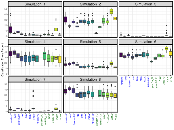
Figure 1: Classification errors for simulations 1 to 8 ($n=100$). Naïve Bayes methods in green.

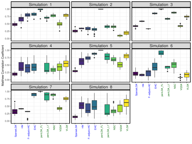
Figure 2: Matthews correlation for simulations 1 to 8 ($n=100$). Naïve Bayes methods in green.

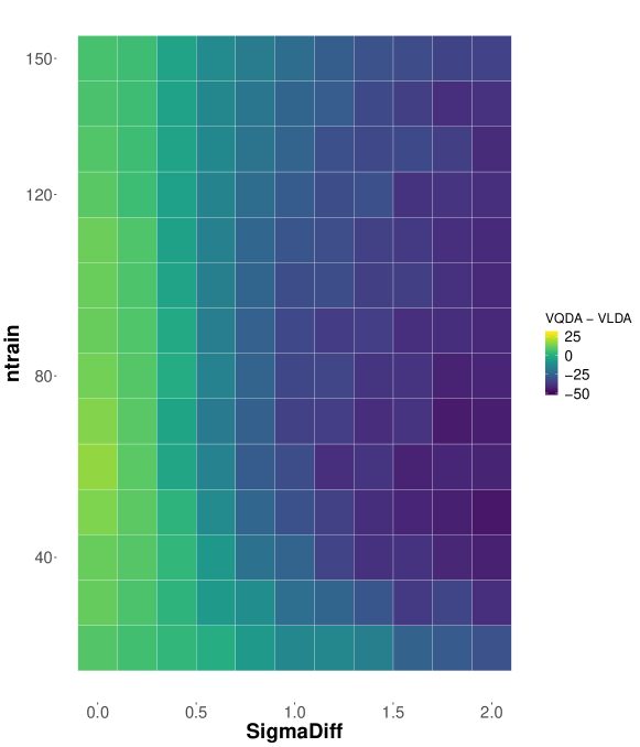
Figure 3: Difference in classification errors (VQDA $-$ VLDA) for varying $n$ and $\Delta_{\sigma}$ over 25 reps. ($p_{1}=25$)

6.4 Simulation results

Boxplots of classification errors and MCCs for simulations 1 to 8 may be found in Figures 1 and 2. Summary statistics of all simulations are provided in Tables 1 to 4 in Electronic Supplementary Material 2. Since penLDA-FL requires the variables to have a linear ordering structure, we have left it out of the comparisons for the simulations setting with randomly drawn means (4, 8, 12 and 16).

VLDA achieved comparatively good classification error performance under the independence (average rank $=6.3$) and local $AR(1)$ correlation structures (average rank $=5.5$). However, the classifier performed rather poorly under the global correlation (average rank $=7.3$) and uniform correlation structure (average rank $=11.5$). Therefore, it is evident that VLDA is robust to a mild violation of the naïve Bayes assumption but is less reliable for classifying data with moderate or strong correlation structure.

Both proposed models also seem to perform relatively better than all other classifiers when the true mean differences is sparse, i.e. $p_{1}/p\leq 10\%$ (simulations 1, 4, 5 and 8) under independent and weak correlation. This is due to the strong global penalty $b_{\gamma}$ imposed on all variable selection probabilities. When the signal strengths are weak (simulations 2 and 6), VLDA did not perform as well in classification error. This may be attributed to the corresponding poor performance in variable selection. Its poor ability to identify weak signals is explained by observing that the cake priors for the mean difference $\mu_{j1}-\mu_{j0}$ is a scale mixture of normals with the log-normal hyperprior on the scale parameter. Although the log-normal distribution is regarded as heavy-tailed in some textbooks, its tail mass is not heavy enough to facilitate the weak signals to overcome the $b_{\gamma}$-global penalty effect. An example of a hyperprior that preserves weak signals from being masked by the global penalty is the half-Cauchy distribution as reported by Carvalho et al. (2010). In contrast, penLDA-L1 performed very well in simulations 2 and 6 due to ability of lasso estimators in picking up weak signals as explained in Fan and Lv (2010).

As for variable selection performance in non-weak signal settings, VLDA performed robustly well even under moderate or strong correlation structure. It is notable that the good performance in variable selection does not translate to good classification performance. This may be in line with the observations made by Mai et al. (2012) that distinguished between signal variables and discriminative variables. Through several examples, the authors showed that it is the identification of discriminative variables, and not signal variables, that lead to better classification performance for LDA models.

By changing the group-conditional variances in each setting to create heterogeneous variance settings, VQDA outperformed VLDA and yielded lower classification error than the other classifiers for independent and weak correlation structure (results omitted from paper). This finding leads us to the follow-up question: how large should the difference in group-conditional variances be for us to choose VQDA over VLDA as our preferred model? We performed further simulations to compare our two proposed models under various regimes of difference in group-conditionals SDs $\Delta_{\sigma}$ and training sample size $n$ over 25 repetitions. Details on the simulation settings and results are summarised in Section 1 of Electronic Supplementary Material 2 and Figure 3 of this manuscript. Based on Figure 3 we found that VLDA performs better than VQDA when $\Delta_{\sigma}\leq 0.4$. However, as $n$ increases, the required $\Delta_{\sigma}$ for VQDA to perform better than VLDA decreases. When $\Delta_{\sigma}\geq 1.6$, VQDA performs better than VLDA even for small $n$ (dark blue patches on the right of each panel). A similar pattern in classification error differences is observed for any $p_{1}\geq 10$. These findings are similar to those reported in Marks and Dunn (1974) and Zavorka and Perrett (2014). Based on this comparison, one should consider the severity of violation in the homogeneity of variance assumption and the training sample size when choosing between VLDA or VQDA.

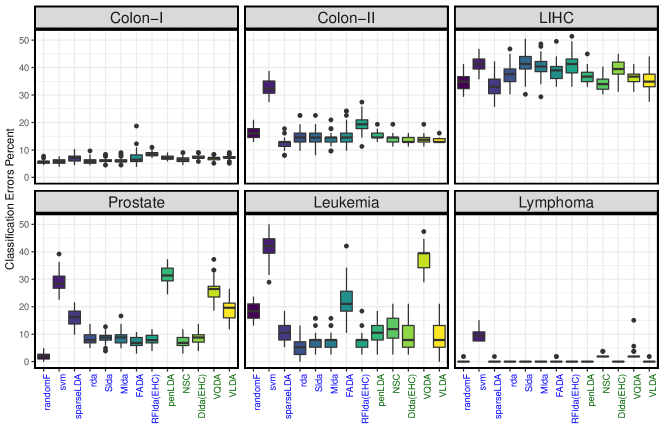
Figure 4: 5-fold CV classification errors for genomics datasets (50 reps). Naïve Bayes methods in green.

6.5 Gene expression datasets

The classifiers are also compared using six gene expression datasets. The description of the datasets may be found in the rest of this subsection. Since the subset of truly discriminative variables are unknown for each dataset, we shall omit the comparison of the variable selection performance. A filtering step is applied to leukemia (Golub et al., 1999), colon I (Jorissen et al., 2008), and TCGA-LIHC (Erickson et al., 2016) datasets to remove genes with mostly $0$ readings. We then standardised each of the six datasets to obtain $z_{ij}=(x_{ij}-\widetilde{\mu}_{j})/s_{j}$ where $x_{ij}$ is the gene $j$ reading for observation $i$, $\widetilde{\mu}_{j}$ is the sample mean of gene $j$ and $s_{j}$ is the sample standard deviation. This standardisation procedure is similar to the one in Dudoit et al. (2002). A 5-fold cross validation over 50 repetitions is performed.

The total number of misclassifications at each iteration is summed across the 5 CV sub-iterations to compare performance between the classifiers. The classification errors and computational time are presented in Figure 4 here and Table 6 of Electronic Supplementary Material 2 respectively.

Colorectal cancer dataset I: This colon cancer dataset is sourced from Bioconductor and has been analysed by Jorissen et al. (2008). The dataset consist of $n=155$ observations of Affymetrix oligonucleotide arrays. The response variable is whether the tumour exhibited microsatellite instability, among which we have 78 microsatellite instable (MSI) tumours and 77 microsatellite stable (MSS) tumours. We implemented a filtering step that excludes genes with within-class outliers that are either 3 IQR above or below the median. This leaves us with $p=8212$ genes.

Colorectal cancer dataset II: This colon cancer dataset is made available by Alon et al. (1999). For convenience, we use the version of the dataset that is found in the rda package. The dataset consist of $n=62$ observations of Affymetrix oligonucleotide arrays. The response variable is cell type, among which we have 40 tumour cells and 22 normal cells. After several pre-filtering steps by Guo et al. (2007), we have $p=2000$ genes that remain for classification.

TCGA-LIHC dataset: The Cancer Genome Atlas Liver Hepatocellular Carcinoma (TCGA-LIHC) dataset is a collection of clinical, genetic and pathological data residing in the Genomic Data Commons (GDC) Data Portal and is made publicly available (Erickson et al., 2016). The data underwent pre-processing to remove genes with IQR $\leq 0.3$ and the $\text{log}_{2}(1+\text{FPKM})$ transformation is taken. Patients whose survival time are lesser the the 20th percentile are considered as poor prognosis ($n_{\text{poor}}=47$) while patients with survival time greater than 80th percentile are labelled as good prognosis ($n_{\text{good}}=62$). Patients who belong to neither survival category were removed from the analysis. This leaves us with $n=109$ observations of $15681$ RNA-seq readings.

Prostate cancer dataset: The prostate cancer dataset is made available by Singh et al. (2002). For convenience, we use the version of the dataset that is found in the sda package. The dataset consist of $n=102$ observations of Affymetrix oligonucleotide arrays. The response variable is cell type, among which we have 52 tumour cells and 50 normal cells from tissue samples obtained from patients treated with radical prostatectomy. After several pre-filtering steps by Ahdesmäki and Strimmer (2010), we have $p=6033$ genes that remain for classification.

Leukemia dataset: The leukemia dataset is made available by Golub et al. (1999). For convenience, we use the version of the dataset that is found in the plsgenomics package. The dataset consist of $n=38$ observations of Affymetrix oligonucleotide arrays. The response variable is leukemia type, among which we have 27 ALL type and 50 AML type leukemia samples. After removing genes with low variation $\leq 0.35$, we have $p=2440$ genes for classification.

Lymphoma dataset: The lymphoma dataset is made available by Alizadeh et al. (2000). For convenience, we use the version of the dataset that is found in the spls package. The dataset consist of 62 samples of 3 variants of lymphoma. Since our proposed model is suitable only for binary classification, we classify a subset of the data consisting of $n=53$ samples of which 42 are DLBCL-type and 11 are CLL-type lymphoma. A total of $p=4026$ genes are used for classification.

6.6 Gene expression dataset results

Though VLDA is not the best performing classifier for any of the datasets in terms of classification accuracy, its classification errors is within a reasonable range from the best performing ones in all datasets except for prostate cancer. In fact, it is ranked among the top 4 classifiers for both colon II and Leukemia datasets, bearing in mind that it achieved this level of classification accuracy at a computational speed of 104 to 867 times faster (based on leukemia dataset) than other the other top classifiers (see Table 4 of Electronic Supplementary Material 2). We acknowledge that the performance of our proposed model is less than satisfactory in the prostate cancer dataset.

VLDA outperformed VQDA in all datasets except for colon I which provides some evidence for the robustness of LDA methods for analysing gene expression datasets.

The performance of the naïve Bayes classifiers are generally close to non-naïve Bayes classifiers. This indicative of the lack of a strong correlation structure in these datasets.

7 Limitations and conclusion

We have proposed a fast classifier that integrates two common objectives in high dimensional data analysis: variable selection and classification. The Bayesian framework of the classifier lends a two fold-advantage to the classifier, provided priors are chosen according to the recommended settings in this paper. Firstly, it leads us to a variable selection rule that aligns with the multiple hypothesis testing paradigm. Although our algorithm may be not asymptotically optimal, we are still able to establish consistency of the variable selection rule under a non-polynomial growth rate for the number of variables. Secondly, the resultant variable selection and classification rules are functions of the their respective frequentist rules, and hence would show high concordance with frequentist results. The classifier is also capable of yielding variable selection and classification results that are comparable to non-naïve Bayes DA models under a weak correlation structure. Furthermore, this is obtained at a very small fraction of the computational cost incurred by these other DA models.

The speed of our proposed classifiers positions them as a useful exploratory analysis tool. In bioinformatics, such high speed algorithms may be deployed to mine through a large number of datasets for the purpose of finding new potential markers.

We made the assumption that the variables are pairwise independent. This assumption is strong and has two implications. First, the classifier may not yield reliable classification results for moderately or strongly correlated dataset. If there is a need to classify highly correlated data with VaDA, one may employ a de-correlation technique that preserves the original dimension of the variable matrix $\mathbf{X}$ such as the latent factor method proposed in Friguet et al. (2009). A study of our classifiers’ performance after an implementation of de-correlation techniques is beyond the scope of our paper. Secondly, we have established our asymptotic results under the condition that the variables are truly independent. A full investigation into the asymptotic behaviour of VLDA under a non-independent correlation structure will be pursued as future research.

Table 3  Iterative scheme for obtaining the parameters in the optimal densities $q\*(\boldsymbol{\gamma},y_{n+1},\ldots,y_{n+m})$ in VQDA
Require: For each $j$, initialise $w_{j}^{(0)}$ with a number in $[0,1]$.
while $||{\bf w}^{(t)}-{\bf w}^{(t-1)}||^{2}$ is greater than $\epsilon$ do
At iteration $t$,
1: $\eta_{j}^{(t)}\leftarrow\log({\bf 1}^{T}{\bf w}_{-j}^{(t-1)}+1)-\log\big{\{}p-{\bf 1}^{T}{\bf w}_{-j}^{(t-1)}-1+b_{\gamma}(r,\kappa)\big{\}}+\tfrac{1}{2}\log(\tfrac{n_{1}n_{0}}{2})$
$\;\;\;\;\;\;\;\;\;\;\;\;\;\;+\xi(\tfrac{n_{1}}{2})+\xi(\tfrac{n_{0}}{2})-\xi(\tfrac{n}{2})-\tfrac{3}{2}\log(n+1)+\tfrac{1}{2}(n+1)\log(\widehat{\sigma}_{j}^{2})-\tfrac{n_{1}}{2}\log(\widehat{\sigma}_{j1}^{2})-\tfrac{n_{0}}{2}\log(\widehat{\sigma}_{j0}^{2})$
2: $w_{j}^{(t)}\leftarrow\text{expit}(\eta_{j}^{(t)})$
Upon convergence of ${\bf w}$, compute for $i=1,\ldots,m$
3: $\widetilde{y}_{i}\leftarrow\text{expit}\bigg{[}\log\big{(}\tfrac{n_{1}}{n_{0}}\big{)}+{\bf 1}^{T}{\bf w}\big{\{}\log\Gamma(\tfrac{n_{1}+1}{2})-\log\Gamma(\tfrac{n_{1}}{2})+\log\Gamma(\tfrac{n_{0}+1}{2})-\log\Gamma(\tfrac{n_{0}}{2})\big{\}}$
$\hskip 59.75095pt+\tfrac{1}{2}{\bf w}^{T}\Big{\{}\log{\boldsymbol{\phi}}({\bf x}_{n+i};\widehat{{\boldsymbol{\mu}}}_{1},\widehat{{\boldsymbol{\sigma}}}_{1}^{2})-\log{\boldsymbol{\phi}}({\bf x}_{n+i};\widehat{{\boldsymbol{\mu}}}_{0},\widehat{{\boldsymbol{\sigma}}}_{0}^{2})\Big{\}}\bigg{]}$

Despite its limitations, we believe that VaDA is a computationally-efficient option for analysing most high dimensional datasets.

Disclosure of potential conflicts of interest

Conflict of Interest: The authors declare that they have no conflict of interest.

Appendix

VQDA derivations

In the VQDA setting ($\sigma_{j1}^{2}\neq\sigma_{j0}^{2}$) the posterior distribution of $\gamma_{j}$ given ${\mathcal{D}}$ and ${\bf x}_{n+1}$ may be expressed as

$$p(\gamma_{j}\;|\;{\mathcal{D}},{\bf x}_{n+1})=\frac{p(\gamma_{j},{\mathcal{D}},{\bf x}_{n+1})}{p({\mathcal{D}},{\bf x}_{n+1})}.$$

By letting $h\rightarrow\infty$, the marginal likelihood of the data in the denominator is of the same form as equation (9)

with the exception that

$${\boldsymbol{\theta}}_{1}=({\boldsymbol{\mu}}_{1},{\boldsymbol{\mu}}_{0},{\boldsymbol{\mu}},{\boldsymbol{\sigma}}_{1}^{2},{\boldsymbol{\sigma}}_{0}^{2},{\boldsymbol{\sigma}}^{2},\rho_{y},\rho_{\gamma}),$$

and

$$\lambda_{\text{LRT}} (\widetilde{{\bf x}}_{j},x_{n+1,j},{\bf y},y_{n+1})$$

$$=(n+1)\log(\widehat{\sigma}_{j}^{2})-(n_{1}+y_{n+1})\log(\widehat{\sigma}_{j1}^{2})$$

$$\hskip 14.22636pt-(n_{0}+1-y_{n+1})\log(\widehat{\sigma}_{j0}^{2}),$$

where

$$\widehat{\sigma}_{j1}^{2}=\tfrac{1}{n_{1}+y_{n+1}}\bigg{[}||{\bf y}^{T}\{\widetilde{{\bf x}}_{j}-\widehat{\mu}_{j1}{\bf 1}\}||^{2}$$

$$\hskip 73.97733pt+y_{n+1}(x_{n+1,j}-\widehat{\mu}_{j1})^{2}\bigg{]},$$

$$\widehat{\sigma}_{j0}^{2}=\tfrac{1}{n_{0}+1-y_{n+1}}\bigg{[}||({\bf 1}-{\bf y})^{T}\{\widetilde{{\bf x}}_{j}-\widehat{\mu}_{j0}{\bf 1}\}||^{2}$$

$$\hskip 76.82234pt+(1-y_{n+1})(x_{n+1,j}-\widehat{\mu}_{j0})^{2}\bigg{]},$$

and the $j^{\mbox{\scriptsize th}}$ entry of ${\boldsymbol{\lambda}}_{\mbox{\scriptsize Bayes}}$ is (as $h\rightarrow\infty$)

$$\lambda_{\mbox{\scriptsize Bayes}}(\widetilde{{\bf x}}_{j},x_{n+1,j},{\bf y},y_{n+1})$$

$$\rightarrow\lambda_{\mbox{\scriptsize LRT}}(\widetilde{{\bf x}}_{j},x_{n+1,j},{\bf y},y_{n+1})+\log(n_{1}+y_{n+1})$$

$$\hskip 11.38092pt+\log(n_{0}+1-y_{n+1})-\log(2)-3\log(n+1)$$

$$\hskip 11.38092pt-2\xi\{(n+1)/2\}+2\xi\{(n_{1}+y_{n+1})/2\}$$

$$\hskip 11.38092pt+2\xi\{(n_{0}+1-y_{n+1})/2\},$$

$$=\lambda_{\mbox{\scriptsize LRT}}(\widetilde{{\bf x}}_{j},x_{n+1,j},{\bf y},y_{n+1})-2\log(n+1)$$

$$\hskip 8.5359pt+O(n_{0}^{-1}+n_{1}^{-1}),$$

where $\xi(x)=\log\Gamma(x)+x-x\log(x)-\tfrac{1}{2}\log(2\pi)$. Since the calculation of the marginal likelihood involves a combinatorial sum over $2^{p+1}$ binary combinations, exact Bayesian inference is also computationally impractical in the VQDA setting.

Similar to VLDA, we will use RCVB to approximate the posterior $p({\boldsymbol{\gamma}},y_{n+1}|{\bf x},{\bf x}_{n+1},{\bf y})$ by

$$q(y_{n+1},{\boldsymbol{\gamma}})=q(y_{n+1})\prod_{j=1}^{p}q_{j}(\gamma_{j}).$$

This yields the approximate posterior for $\gamma_{j}$ as

$$q_{j}(\gamma_{j})\propto\int\exp\big{[}{\mathbb{E}}_{-q_{j}}\{\log p({\mathcal{D}},{\bf x}_{n+1},y_{n+1},{\boldsymbol{\gamma}},{\boldsymbol{\theta}}_{1})\}\big{]}\text{d}{\boldsymbol{\theta}}_{1},$$

$$\propto\exp\bigg{[}{\mathbb{E}}_{-q_{j}}\Big{\{}\log{\mathcal{B}}(a_{\gamma}+{\bf 1}^{T}{\boldsymbol{\gamma}},b_{\gamma}+p-{\bf 1}^{T}{\boldsymbol{\gamma}})\Big{\}}$$

$$\hskip 34.1433pt+\tfrac{\gamma_{j}}{2}{\mathbb{E}}_{-q_{j}}\Big{\{}{\boldsymbol{\lambda}}_{\mbox{\scriptsize Bayes}}(\widetilde{{\bf x}}_{j},x_{n+1,j},{\bf y},y_{n+1})\Big{\}}\bigg{]}.$$

For a sufficiently large $n$, we can avoid the need to evaluate the expectation ${\mathbb{E}}_{-q_{j}}\Big{\{}{\boldsymbol{\lambda}}_{\mbox{\scriptsize Bayes}}(\widetilde{{\bf x}}_{j},x_{n+1,j},{\bf y},y_{n+1})\Big{\}}$ by applying Taylor’s expansion to obtain the approximation

$${\mathbb{E}}_{-q_{j}}\log(a_{\gamma}+{\bf 1}^{T}{\boldsymbol{\gamma}}_{-j})\approx\log(a_{\gamma}+{\bf 1}^{T}{\bf w}_{-j}),$$

$${\mathbb{E}}_{-q_{j}}\log(b_{\gamma}+p-{\bf 1}^{T}{\boldsymbol{\gamma}}_{-j}-1)$$

$$\hskip 22.76219pt\approx\log(b_{\gamma}+p-{\bf 1}^{T}{\bf w}_{-j}-1),$$

$$\widehat{\sigma}_{j1}^{2}\approx\tfrac{1}{n_{1}}||{\bf y}^{T}\{\widetilde{{\bf x}}_{j}-\widehat{\mu}_{j1}{\bf 1}\}||^{2},$$

$$\widehat{\sigma}_{j0}^{2}\approx\tfrac{1}{n_{0}}||({\bf 1}-{\bf y})^{T}\{\widetilde{{\bf x}}_{j}-\widehat{\mu}_{j0}{\bf 1}\}||^{2},$$

$$\widehat{\sigma}_{j}^{2}\approx\tfrac{1}{n}||\widetilde{{\bf x}}_{j}-\widehat{\mu}_{j}{\bf 1}||^{2},$$

$$\widehat{\mu}_{j1}\approx\tfrac{1}{n_{1}}{\bf y}^{T}\widetilde{{\bf x}}_{j},\;\;\widehat{\mu}_{j0}\approx\tfrac{1}{n_{0}}({\bf 1}-{\bf y})^{T}\widetilde{{\bf x}}_{j},\;\;\widehat{\mu}_{j}\approx\tfrac{1}{n}{\bf 1}^{T}\widetilde{{\bf x}}_{j},$$ (16)

and, similar to VLDA, ${\boldsymbol{\lambda}}_{\mbox{\scriptsize Bayes}}$ does not depend on the new observation $({\bf x}_{n+1},y_{n+1})$. By using the approximation in (VQDA derivations), we have

$$w_{j}=\frac{q_{j}(\gamma_{j}=1)}{q_{j}(\gamma_{j}=1)+q_{j}(\gamma_{j}=0)},$$

$$\approx\text{expit}\bigg{[}\log(a_{\gamma}+{\bf 1}^{T}{\bf w}_{-j})-\log(b_{\gamma}+p-{\bf 1}^{T}{\bf w}_{-j}-1)$$

$$\hskip 39.83385pt+\tfrac{1}{2}\log(\tfrac{n_{1}n_{0}}{2})+\xi(\tfrac{n_{1}}{2})+\xi(\tfrac{n_{0}}{2})-\xi(\tfrac{n}{2})$$

$$\hskip 39.83385pt-\tfrac{3}{2}\log(n+1)+\tfrac{1}{2}\lambda_{\mbox{\scriptsize LRT}}(\widetilde{{\bf x}}_{j},y_{n+1})\bigg{]},$$

$$=\text{expit}\bigg{[}\text{penalty}_{QDA,j}+\tfrac{1}{2}\lambda_{\mbox{\scriptsize LRT}}(\widetilde{{\bf x}}_{j},y_{n+1})\bigg{]},$$

To obtain the approximate density for $y_{n+1}$, we integrate analytically over ${\boldsymbol{\theta}}_{1}$ to obtain

$$q(y_{n+1})\propto\int\exp\big{[}{\mathbb{E}}_{-y}\{\log p({\mathcal{D}},{\bf x}_{n+1},y_{n+1},{\boldsymbol{\gamma}},{\boldsymbol{\theta}}_{1})\}\big{]}\text{d}{\boldsymbol{\theta}}_{1},$$

$$\propto\exp\bigg{[}\log{\mathcal{B}}(a_{y}+n_{1}+y_{n+1},b_{y}+n_{0}+1-y_{n+1})$$

$$\hskip 34.1433pt+{\bf 1}^{T}{\bf w}\Big{\{}\log\Gamma(\tfrac{n_{1}+y_{n+1}}{2})+\log\Gamma(\tfrac{n_{0}+1-y_{n+1}}{2})\Big{\}}$$

$$\hskip 8.53581pt+\tfrac{1}{2}{\bf w}^{T}\Big{\{}\log{\boldsymbol{\phi}}({\bf x}_{n+1};\widehat{{\boldsymbol{\mu}}}_{1},\widehat{{\boldsymbol{\sigma}}}_{1}^{2})-\log{\boldsymbol{\phi}}({\bf x}_{n+1};\widehat{{\boldsymbol{\mu}}}_{0},\widehat{{\boldsymbol{\sigma}}}_{0}^{2})\Big{\}}\bigg{]},$$

where the $j^{\mbox{\scriptsize th}}$ element of the $p\times 1$ vector ${\boldsymbol{\phi}}({\bf x}_{n+1};\widehat{{\boldsymbol{\mu}}}_{k},\widehat{{\boldsymbol{\sigma}}}_{k}^{2})$ is the Gaussian density

$$\phi(x_{n+1,j};\widehat{\mu}_{jk},\widehat{\sigma}_{jk}^{2}),$$

and the $\log$ prefix denotes an element-wise $\log$ of a vector.

In the general case with $m$ new observations, we may apply Taylor’s expansion results from (VQDA derivations) to compute the approximate classification probability for $y_{n+i}$ as

$$\widetilde{y}_{i}=\frac{q(y_{n+i}=1)}{q(y_{n+i}=1)+q(y_{n+i}=0)},$$

$$\hskip 8.53581pt\approx\text{expit}\bigg{[}\log\big{(}\tfrac{n_{1}}{n_{0}}\big{)}+{\bf 1}^{T}{\bf w}\big{\{}\log\Gamma(\tfrac{n_{1}+1}{2})-\log\Gamma(\tfrac{n_{1}}{2})$$

$$\hskip 99.58464pt+\log\Gamma(\tfrac{n_{0}+1}{2})-\log\Gamma(\tfrac{n_{0}}{2})\big{\}}$$

$$+\tfrac{1}{2}{\bf w}^{T}\Big{\{}\log{\boldsymbol{\phi}}({\bf x}_{n+i};\widehat{{\boldsymbol{\mu}}}_{1},\widehat{{\boldsymbol{\sigma}}}_{1}^{2})-\log{\boldsymbol{\phi}}({\bf x}_{n+i};\widehat{{\boldsymbol{\mu}}}_{0},\widehat{{\boldsymbol{\sigma}}}_{0}^{2})\Big{\}}\bigg{]}.$$

The RCVB alogrithm for VQDA may be found in Table 3.

References

- Ahdesmäki and Strimmer (2010) Ahdesmäki, M., Strimmer, K.: Feature selection in omics prediction problems using CAT score and false discovery rate control. The Annals of Applied Statistics 4(1), 503–519 (2010)
- Alizadeh et al. (2000) Alizadeh, A., Eisen, M., Davis, R., Ma, C., Lossos, I., Rosenwald, A., Boldrick, J., Sabet, H., Tran, T., Yu, X., Powell, J., Yang, L., Marti, G., Moore, T., Hudson, J.J., Lu, L., Lewis, D., Tibshirani, R., Sherlock, G., Chan, W., Greiner, T., Weisenburger, D., Armitage, J., Warnke, R., Levy, R., Wilson, W., Grever, M., Byrd, J., Botstein, D., Brown, P., Staudt, L.: Distinct types of diffuse large b-cell lymphoma identified by gene expression profiling. Nature 403, 503–511 (2000)
- Alon et al. (1999) Alon, U., Barkai, N., Notterman, D., Gish, K., Ybarra, S., Mack, D., AJ, L.: Broad patterns of gene expression revealed by clustering analysis of tumor and normal colon tissues probed by oligonucleotide arrays. Proceedings of the National Academy of Sciences 96(12), 6745–6750 (1999)
- Benjamini and Daniel (2001) Benjamini, Y., Daniel, Y.: The control of the false discovery rate in multiple testing under dependency. The Annals of Statistics 29(4), 1165––1188 (2001)
- Benjamini and Hochberg (1995) Benjamini, Y., Hochberg, Y.: Controlling the false discovery rate: a practical and powerful approach to multiple testing. Journal of the Royal Statistical Society, Series B 57(1), 289––300 (1995)
- Bickel and Levina (2004) Bickel, P.J., Levina, E.: Some theory for Fisher’s linear discriminant function, ‘naïve Bayes’ and some alternatives when there are many more variables than observations. Bernoulli 10(6), 989–1010 (2004)
- Blei and Jordan (2006) Blei, D.M., Jordan, M.I.: Variational inference for Dirichlet processes. Bayesian Analysis 1(1), 121–144 (2006)
- Blei et al. (2017) Blei, D.M., Kucukelbir, A., McAuliffe, J.D.: Variational inference: A review for statisticians. Journal of American Statistical Association 112(518), 859–877 (2017)
- Bonferroni (1936) Bonferroni, C.E.: Teoria statistica delle classi e calcolo delle probabilità. Pubblicazioni del R Istituto Superiore di Scienze Economiche e Commerciali di Firenze (1936)
- Breiman (2001) Breiman, L.: Random forests. Machine Learning 45(1), 5–32 (2001)
- Cai and Liu (2011) Cai, T., Liu, W.: A direct estimation approach to sparse linear discriminant analysis. Journal of the American Statistical Association 106(496), 1566–1577 (2011)
- Carvalho et al. (2010) Carvalho, C.M., Polson, N.G., Scott, J.G.: The horseshoe estimator for sparse signals. Biometrika 97(2), 465–280 (2010)
- Chen and Feng (2014) Chen, Y., Feng, J.: Efficient method for Moore-Penrose inverse problems involving symmetric structrue based on group theory. Journal of Computing in Civil Engineering 28(2), 182–190 (2014)
- Chicco (2017) Chicco, D.: Ten quick tips for machine learning in computational biology. BioData Mining 10(35), 1–17 (2017)
- Clemmensen (2013) Clemmensen, L.: On discriminant analysis techniques and correlation structures in high dimensions. Kgs. Lyngby: Technical University of Denmark (DTU). Technical Report-2013 (4) (2013)
- Clemmensen and Kuhn (2016) Clemmensen, L., Kuhn, M.: sparseLDA: Sparse Discriminant Analysis (2016). R package version 0.1-9
- Clemmensen et al. (2011) Clemmensen, L., Witten, D., Hastie, T., Ersboll, B.: Sparse discriminant analysis. Technometrics 53(4), 406–413 (2011)
- Cortes and Vapnik (1995) Cortes, C., Vapnik, V.: Support-vector networks. Machine Learning 20(3), 273–297 (1995)
- Courrieu (2005) Courrieu, P.: Fast computation of Moore-Penrose inverse matrices. Neural Information Processing - Letters and Reviews 8(2), 25–29 (2005)
- Craig-Shapiro et al. (2011) Craig-Shapiro, R., Kuhn, M., Xiong, C., Pickering, E.H., Liu, J., Misko, T.P., Perrin, R.J., Bales, K.R., Soares, H., Fagan, A.M., David, M.H.: Multiplexed immunoassay panel identifies novel CSF biomarkers for Alzheimer’s disease diagnosis and prognosis. PLoS ONE p. e18850 (2011)
- Donoho and Jin (2004) Donoho, D., Jin, J.: Higher criticism for detecting sparse heterogeneous mixtures. The Annals of Statistics 32(3), 962––994 (2004)
- Donoho and Jin (2008) Donoho, D., Jin, J.: Higher criticism thresholding. optimal feature selection when useful features are rare and weak. Proceedings of the National Academy of Sciences 105(39), 14790–14795 (2008)
- Duarte Silva (2011) Duarte Silva, P.A.: Two group classification with high-dimensional correlated data: a factor model approach. Computational Statistics and Data Analysis 55(11), 2975–2990 (2011)
- Duarte Silva (2015) Duarte Silva, P.A.: HiDimDA: High dimensional discriminant analysis (2015). R package version 0.2-4
- Dudoit et al. (2002) Dudoit, S., Fridyland, J., Speed, T.P.: Comparison of discrimination methods for classification of tumours using gene expression data. Journal of American Statistical Association 97(457), 77–87 (2002)
- Eddelbuettel (2013) Eddelbuettel, D.: Seamless R and C++ integration with Rcpp. Springer (2013)
- Erickson et al. (2016) Erickson, B.J., Kirk, S., Lee, Y., Bathe, O., Kearns, M., Gerdes, C., Rieger-Christ, K., Lemmerman, J.: Radiology Data from The Cancer Genome Atlas Liver Hepatocellular Carcinoma [TCGA-LIHC] collection. The Cancer Imaging Archive. (2016)
- Fan and Fan (2008) Fan, J., Fan, Y.: High-dimensional classification using features annealed independence rules. The Annals of Statistics 36(6), 2605–2637 (2008)
- Fan and Lv (2010) Fan, J., Lv, J.: A selective overview of variable selection in high dimensional feature space. Statistica Sinica 20(1), 101–148 (2010)
- Fernández-Delgado et al. (2014) Fernández-Delgado, M., Cernadas, E., Barro, S.: Do we need hundreds of classifiers to solve real world classification problems? Journal of Machine Learning 15, 3133–3181 (2014)
- Fisher (1936) Fisher, R.A.: The use of multiple measurements in taxonomic problems. Annals of Eugenics 7(2), 179–188 (1936)
- Fisher and Sun (2011) Fisher, T., Sun, X.: Improved stein-type shrinkage estimators for the high-dimensional multivariate normal covariance matrix. Computational Statistics and Data Analysis 55(1), 1909–1918 (2011)
- Friedman (1989) Friedman, J.H.: Regularized discriminant analysis. Journal of the American Statistical Association 84(405), 165–175 (1989)
- Friguet et al. (2009) Friguet, C., Kloareg, M., Causeur, D.: A factor model approach to multiple testing under dependence. Journal of the American Statistical Association 104(488), 1406–1415 (2009)
- Golub et al. (1999) Golub, T., Slonim, D., Tamayo, P., Huard, C., Gaasenbeek, M., Mesirov, J.: Molecular classification of cancer: Class discovery and class prediction by gene expression monitoring. Science 286(5439), 531–537 (1999)
- Guo et al. (2007) Guo, Y., Hastie, T., Tibshirani, R.: Regularized linear discriminant analysis and its application in microarrays. Biostatistics 8(1), 86–100 (2007)
- Guo et al. (2018) Guo, Y., Hastie, T., Tibshirani, R.: rda: Shrunken Centroids Regularized Discriminant Analysis (2018). R package version 1.0.2-2.1
- Hastie et al. (2014) Hastie, T., Tibshirani, R., Narasimhan, B., Chu, G.: pamr: Prediction analysis for microarrays (2014). R package version 1.55
- Helleputte (2017) Helleputte, T.: LiblineaR: Linear Predictive Models Based on the LIBLINEAR C/C++ Library (2017). R package version 2.10-8
- Jorissen et al. (2008) Jorissen, R.N., Lipton, L., Gibbs, P., Chapman, M., Desai, J., Jones, I.T., Yeatman, T.J., East, P., Tomlinson, I.P., Verspaget, H.W., Aaltonen, L.A., Kruhoffer, M., Orntoft, T.F., Andersen, C.L., Sieber, O.M.: DNA copy-number alterations underlie gene expression differences between microsatellite stable and unstable colorectal cancers. Clinical Cancer Research 14(24), 8061–8069 (2008)
- Kuhn et al. (2019) Kuhn, M., Wing, J., Weston, S., Williams, A., Keefer, C., Engelhardt, A., Cooper, T., Mayer, Z., Kenkel, B., Benesty, M., Lescarbeau, R., Ziem, A., Scrucca, L., Tang, Y., Candan, C., Hunt, T.: caret: Classification and Regression Training (2019). R package version 6.0-84
- Liu et al. (2005) Liu, J.J., Cutler, G., Li, W., Pan, Z., Peng, S., Hoey, T., Chen, L., Ling, X.B.: Multiclass cancer classification and biomarker discovery using GA-based algorithms. Bioinformatics 21(11), 2691––2697 (2005)
- Luts and Ormerod (2014) Luts, J., Ormerod, J.T.: Mean field variational Bayesian inference for support vector machine classification. Computational Statistics and Data Analysis 73, 163–176 (2014)
- Mai et al. (2012) Mai, Q., Zou, H., Yuan, M.: A direct approach to sparse discriminant analysis in ultra-high dimensions. Biometrika 99(1), 29–42 (2012)
- Marks and Dunn (1974) Marks, S., Dunn, O.: Discriminant functions when covariance matrices are unequal. Journal of the American Statistical Association 69(346), 555–559 (1974)
- Matthews (1975) Matthews, B.W.: Comparison of the predicted and observed secondary structure of T4 phage lysozyme. Biochimica et Biophysica Acta (BBA) - Protein Structure 405(2), 442–451 (1975)
- Ormerod et al. (2017) Ormerod, J.T., Stewart, M., Yu, W., Romanes, S.: Bayesian hypothesis test with diffused priors: Can we have our cake and eat it too? ArXiv (2017)
- Ormerod and Wand (2010) Ormerod, J.T., Wand, M.P.: Explaining variational approximations. The American Statistician 64(2), 140–153 (2010)
- Perthame et al. (2016) Perthame, E., Friguet, C., Causeur, D.: Stability of feature selection in classification issues for high-dimensional correlated data. Statistics and Computing 26(4), 783–796 (2016)
- Perthame et al. (2018) Perthame, E., Friguet, C., Causeur, D.: FADA: Variable Selection for Supervised Classification in High Dimension (2018). R package version 1.3.3
- Safo and Ahn (2016) Safo, S.E., Ahn, J.: General sparse multi-class linear discriminant analysis. Computational Statistics and Data Analysis 99, 81–90 (2016)
- Shaffer (1995) Shaffer, J.P.: Multiple hypothesis testing. Annual Review of Psychology 46, 561––584 (1995)
- Shao et al. (2011) Shao, J., Wang, Y., Deng, X., Wang, S.: Sparse linear discriminant analysis with applications to high dimensional data. Annals of Statistics 39(2), 1241–1265 (2011)
- Singh et al. (2002) Singh, D., Febbo, P., Ross, K., Jackson, D., Manola, J., Ladd, C., Tamayo, P., Renshaw, A., DAmico, A., Richie, J., Lander, E., Loda, M., Kantoff, P., Golub, T.: Gene expression correlates of clinical prostate cancer behavior. Cancer cell 1(2), 203–209 (2002)
- Srivastava et al. (2007) Srivastava, S., Gupta, M.R., Frigyik, B.A.: Bayesian quadratic discriminant analysis. Journal of Machine Learning Research 8(Jun), 1277–1305 (2007)
- Storey (2003) Storey, J.D.: The positive false discovery rate: a Bayesian interpretation and the q-value. Annals of Statistics 31(6), 2013––2035 (2003)
- Teh et al. (2007) Teh, Y.W., Newman, D., Welling, M.: A collapsed variational Bayesian inference algorithm for latent Dirichlet allocation. In: Advances in Neural Information Processing Systems, vol. 19, pp. 1353–1360. MIT Press (2007)
- Thomaz et al. (2006) Thomaz, C., Kitani, E., Gillies, D.: A maximum uncertainty lda-based approach for limited sample size problems - with applications to face recognition. Journal of Brazilian Computer Society 12(2), 7–18 (2006)
- Tibshirani et al. (2003) Tibshirani, R., Hastie, T., Narasimhan, B., Chu, G.: Class prediction by nearest shrunken centroids, with applications to DNA microarrays. Statistical Science 18(1), 104–117 (2003)
- van der Maaten and Hinton (2017) van der Maaten, L., Hinton, G.: Visualising data using t-sne. Journal of Machine Learning Research 9, 2579–2605 (2017)
- Wang and Blei (2018) Wang, Y., Blei, D.: Frequentist consistency of variational bayes. Journal of the American Statistical Association 9, 1–15 (2018). doi:10.1080/01621459.2018.1473776
- Witten (2011) Witten, D.: Classification and clustering of sequencing data using a Poisson model. Annals of Applied Statistics 5(4), 2493–2518 (2011)
- Witten (2015) Witten, D.: penalizedLDA: Penalized Classification using Fisher’s Linear Discriminant (2015). R package version 1.1
- Witten and Tibshirani (2011) Witten, D., Tibshirani, R.: Penalized classification using Fisher’s linear discriminant. Journal of Royal Statistical Society Series B 73(5), 754–772 (2011)
- Xu et al. (2009) Xu, P., Brock, G.N., Parrish, R.S.: Modified linear discriminant analysis approaches for classification of high-dimensional microarray data. Computational Statistics and Data Analysis 53, 1674–1687 (2009)
- Zavorka and Perrett (2014) Zavorka, S., Perrett, J.: Minimum sample size considerations for two-group linear and quadratic discriminant analysis with rare populations. Communications in Statistics - Simulation and Computation 43(7), 1726–1739 (2014)
- Zhang and Zhou (2017) Zhang, A., Zhou, H.: Theoretical and computational guarantees of mean field variational inference for community detection. ArXiv (2017)