Gauge-invariant microscopic kinetic theory of superconductivity: application to electromagnetic response of Nambu-Goldstone and Higgs modes

Abstract

We show that the gauge-invariant kinetic equation of superconductivity provides an efficient approach to study the electromagnetic response of the gapless Nambu-Goldstone and gapful Higgs modes on an equal footing. We prove that the Fock energy in the kinetic equation is equivalent to the generalized Ward’s identity. Hence, the gauge invariance directly leads to the charge conservation. Both linear and second-order responses are investigated. The linear response of the Higgs mode vanishes in the long-wave limit. Whereas the linear response of the Nambu-Goldstone mode interacts with the long-range Coulomb interaction, causing the original gapless spectrum lifted up to the plasma frequency as a result of the Anderson-Higgs mechanism, in consistency with the previous works. The second-order response exhibits interesting physics. On one hand, a finite second-order response of the Higgs mode is obtained in the long-wave limit. We reveal that this response, which has been experimentally observed, is attributed solely to the drive effect rather than the widely considered Anderson-pump effect. On the other hand, the second-order response of the Nambu-Goldstone mode, free from the influence of the long-range Coulomb interaction and hence the Anderson-Higgs mechanism, is predicted. We find that both Anderson-pump and drive effects play important role in this response. A tentative scheme to detect this second-order response is proposed.

I Introduction

The collective excitation in the superconducting states has been the focus of study in the field of superconductivity for the past few decades. Two types of collective modes emerge with the generation of the superconducting order parameter $\Delta$: the gapless phase modegi0 ; AK ; Gm1 ; Gm2 ; Ba0 ; pm0 ; pi1 ; pm1 ; pm2 ; pi4 ; gi1 ; Ba9 ; Ba10 ; pm5 and gapful amplitude mode,pm5 ; Am0 ; Am5 ; Am6 ; Am12 ; Am13 which correspond to the fluctuation of phase and amplitude of the order parameter, respectively. Specifically, through the generalized Ward’s identity, Nambu first revealed the existence of a collective gapless excitation in the superconducting states.gi0 It is understood later that this gapless excitation is described as a collective phase mode of the order parameterAK and corresponds to the gapless Goldstone bosons in the field theory by the spontaneous breaking of the continuous $U(1)$ symmetry.Gm1 ; Gm2 After that, the phase mode is further proved by obtaining the effective Lagrangian of the order parameter via the path integral method,pi1 ; pi4 and is now referred to as the Nambu-Goldstone (NG) mode.pm1 ; pm2 ; pi4 ; gi1 ; Ba9 ; Ba10 ; pm5 The counterpart of the phase mode is the amplitude mode,pm5 ; Am0 ; Am6 ; Am12 ; Am13 which is referred to as the Higgs mode due to the similarity of the Higgs bosons in the field theory.Higgs1 ; Higgs2 ; Higgs3 Particularly, a gapful energy spectrum $\omega_{\rm H}=2|\Delta|$ of the Higgs mode in superconductors is predicted in the long-wave limit.pm5 ; Am0 ; Am6 ; Am13

Since the elucidation of the existence of the collective modes in superconductors, a great deal of theoretical efforts have been devoted to their electromagnetic response. Nevertheless, the theoretical studies of the electromagnetic responses of the NG mode and Higgs mode in the literature so far are separated by either fixing the amplitude or overlooking the phase of the order parameter. Moreover, due to the spontaneous breaking of the $U(1)$ symmetry by the generation of the order parameter, it is establishedgi0 ; Ba0 ; gi1 ; Ba9 ; Ba10 that the gauge transformation in the superconducting states contains the superconducting phase $\theta$ of the order parameter, in addition to the standard electromagnetic potential $A_{\mu}=(\phi,{\bf A})$. Nambu pointed outgi0 ; gi1 ; Ba0 via the generalized Ward’s identity that the gauge invariance in the superconducting states is equivalent to the charge conservation. Since the charge conservation is directly related to the electromagnetic properties, the gauge invariance is necessary for the physical description. Nevertheless, a complete gauge-invariant theory for the electromagnetic response of both collective modes is still in progress.

Specifically, with the fixed amplitude of the order parameter, via the Gorkov’s equation,G1 it is first revealed by Ambegaokar and KadanoffAK that the NG mode responds to the electromagnetic field in the linear regime. Nevertheless, this linear response of the NG mode interacts with the long-range Coulomb interaction,AK causing the original gapless energy spectrum lifted up to the high-energy plasma frequency as a result of Anderson-Higgs mechanism.AHM However, for the gauge-invariant approach in Ambegaokar and Kadanoff’s work,AK in order to obtain the NG mode, an additional condition of the charge conservation is required.AKs This seems superfluous since as mentioned above, the presence of the gauge invariance directly implies the charge conservation.gi0 ; gi1 ; Ba0 After that, the Anderson-Higgs mechanism of the NG mode in the linear response is further discussed within the diagrammatic formalism.pm0 ; pm5 ; gi1 ; Ba0 ; Am0 ; gi0 However, due to the difficulty in treating the nonlinear effect in the diagrammatic formalism or the Gorkov’s equation, the nonlinear response of the NG mode is absent in the literature.

The electromagnetic response of the Higgs mode has recently been focused in the second-order regime. This is inspired by the recent experiments,NL7 ; NL8 ; NL9 ; NL10 ; NL11 from which it is realized that the intense THz field can excite the oscillation of the superfluid density in the second-order response. This oscillation so far is attributed to the excitation of the Higgs mode based on the observed resonance when the optical frequency is tuned at the superconducting gap.NL8 ; NL9 ; NL10 Theoretical description for this response has been based on the BlochAm1 ; Am2 ; Am7 ; Am9 ; Am11 ; Am14 ; NL7 ; NL8 ; NL9 ; NL10 ; NL11 or LiouvilleAm3 ; Am4 ; Am8 ; Am10 equation derived in the Anderson pseudospin picture.As The second-order term $A^{2}$ naturally emerges in these descriptions,Am1 ; Am2 ; Am3 ; Am4 ; Am7 ; Am8 ; Am9 ; Am10 ; Am11 ; Am14 ; NL7 ; NL8 ; NL9 ; NL10 ; NL11 causing the pump of the quasiparticle correlation (pump effect) and hence the fluctuation of the order parameter $\Delta$. Then, it is claimed that the Higgs mode is excited. Recently, this description is challenged.symmetry ; GOBE1 ; GOBE2 ; GOBE3 ; GOBE4 Firstly, the symmetry analysissymmetry from the Anderson pseudospin picture implies that with the particle-hole symmetry, the excited fluctuation of the order parameter by the pump effect is the oscillation of its phase. This suggests that the pump effect excites the NG mode rather than the Higgs mode. Secondly, the BlochAm1 ; Am2 ; Am7 ; Am9 ; Am11 ; Am14 ; NL7 ; NL8 ; NL9 ; NL10 ; NL11 or LiouvilleAm3 ; Am4 ; Am8 ; Am10 equation fails in the linear response to describe the optical conductivity since no drive effect (i.e., linear term) is included.GOBE3 ; GOBE4 Thus, these descriptions are insufficient to elucidate the complete physics. Most importantly, with the vector potential alone, the gauge invariance is unsatisfied in the Bloch or Liouville equation in the literature.GOBE1 ; GOBE2 ; GOBE3 ; GOBE4

Very recently, we extend the nonequilibrium $\tau_{0}$-Green-function approach ($\tau_{i}$ are the Pauli matrices in the particle-hole space), which has been very successful in studying the dynamics of the semiconductor opticsGQ2 and spintronics,GQ3 into the dynamics of superconductivity. The equal-time scheme in this approach, corresponding to the instantaneous optical transitionGQ2 in optics and the nonretarded spin precessionGQ3 in spintronics, can naturally be applied into the conventional $s$-wave superconducting states thanks to the BCS equal-time pairing.BCS To retain the gauge invariance, the gauge-invariant $\tau_{0}$-Green function is constructed through the Wilson lineWilson . Then, a gauge-invariant kinetic equation (GIKE) is developed for the electromagnetic response of the superconductivity. As a result of the gauge invariance, both the Anderson-pump and drive effects mentioned above are kept. By following the previous approaches,Am1 ; Am2 ; Am3 ; Am4 ; Am5 ; Am6 ; Am7 ; Am8 ; Am9 ; Am10 ; Am11 ; Am12 ; Am13 ; Am14 ; NL7 ; NL8 ; NL9 ; NL10 ; NL11 i.e., overlooking the NG mode (lifted up to the plasma frequency by the long-range Coulomb interaction), it is shown by the GIKEGOBE1 ; GOBE2 ; GOBE3 ; GOBE4 that instead of the well-studied Anderson-pump effect in the literature,Am1 ; Am2 ; Am7 ; Am9 ; Am11 ; Am14 ; NL7 ; NL8 ; NL9 ; NL10 ; NL11 ; Am3 ; Am4 ; Am8 ; Am10 the second order of the drive effect dominates the second-order response of the Higgs mode. Moreover, in a latest paper,GOBE4 we further show that both superfluid and normal-fluid dynamics are involved in the GIKE, beyond the Boltzmann equation of superconductors in the literatureBa3 ; Bol ; Ba5 which only includes the quasiparticle excitations. Particularly, the equal-time scheme in the GIKE makes it very easy to handle the temporal evolution and microscopic scattering in the superconducting states, in contrast to the conventional Eilenberger transport equation in superconductors which is derived from $\tau_{3}$-Green function and restricted by the normalization condition.Eilen ; Ba7 ; Ba8 ; Ba20 Consequently, in addition to the well-known clean-limit results such as the Ginzburg-Landau equation near $T_{c}$ and the Meissner supercurrent in the magnetic response, from the GIKE, rich physics by the microscopic scattering has been revealed.GOBE4 Specifically, we find there exists a friction between the normal-fluid and superfluid currents and due to this friction, part of the superfluid becomes viscous. Therefore, a three-fluid model with the normal fluid and nonviscous and viscous superfluids is proposed.

In this work, we show that the GIKE developed beforeGOBE1 ; GOBE2 ; GOBE3 ; GOBE4 also provides an efficient approach to study the electromagnetic response of the collective modes in the superconducting states. We first demonstrate that the generalized Ward’s identity by Nambugi0 ; Ba0 is equivalent to the Fock energy in the GIKE. With the complete Fock term, the gauge invariance in the GIKE directly leads to the charge conservation, in contrast to the previous Ambegaokar and Kadanoff’s approachAK where an additional condition of the charge conservation is required to obtain the NG mode. In addition to the Fock term in our previous GIKE,GOBE4 the Hartree one (i.e., the vacuum polarization) is also added in the present work. Then, both linear and second-order responses are investigated. Differing from the previous studies in the literature with either the fixed amplitudeAK ; pi1 ; pm1 ; pm2 ; pi4 ; Ba9 or overlooked phaseAm1 ; Am2 ; Am3 ; Am4 ; Am5 ; Am6 ; Am7 ; Am8 ; Am9 ; Am10 ; Am11 ; Am12 ; Am13 ; Am14 ; NL7 ; NL8 ; NL9 ; NL10 ; NL11 ; GOBE1 ; GOBE2 ; GOBE3 ; GOBE4 of the order parameter, in the present work, the gapless NG and gapful Higgs modes are calculated on an equal footing. Consequently, the contributions from the phase and amplitude modes to the fluctuation of the order parameter, which are ambiguous in the Anderson pseudospin picture as mentioned above, can be directly distinguished in our GIKE approach.

Specifically, the linear response of the NG mode from our GIKE agrees with the previous results in the literature.AK ; Ba0 ; pm0 ; Am0 ; Ba9 ; Ba10 ; pm5 The linear response of the NG mode interacts with the long-range Coulomb interaction, causing the original gapless energy spectrum inside the superconducting gap effectively lifted up to the high-energy plasma frequency far above the gap as a result of Anderson-Higgs mechanism.AHM Consequently, no effective linear response of the NG mode occurs. The origin of the plasma frequency is addressed. The second-order response of the NG mode to the electromagnetic field, which is hard to deal with in the previous approaches in the literature,AK ; Ba0 ; Ba9 ; Ba10 ; pm0 ; pm5 ; Am0 ; pi1 ; pi4 exhibits interesting physics in contrast to the linear one. Specifically, in the second-order regime, we find that the NG mode also responds to the electromagnetic field. Both the Anderson-pump effect and the second order of the drive effect play important role. Particularly, in striking contrast to the linear response above, it is very interesting to find that the second-order response of the NG mode decouples with the long-range Coulomb interaction, and hence maintains the original gapless energy spectrum inside the superconducting gap, free from the influence of the Anderson-Higgs mechanism.AHM The origin of this decoupling is revealed. A tentative scheme to detect the second-order response of the NG mode is also proposed.

As for the Higgs mode, we find that the Higgs mode also responds to the electromagnetic field in the linear regime but this response vanishes in the long-wave limit. A finite response of the Higgs mode in the long-wave limit is obtained in the second-order regime. By further comparing the Anderson-pump and drive effects, we show that the widely considered pump effect in the literatureAm1 ; Am2 ; Am7 ; Am9 ; Am11 ; Am14 ; Am3 ; Am4 ; Am8 ; Am10 ; NL7 ; NL8 ; NL9 ; NL10 ; NL11 ; GOBE1 ; GOBE2 ; GOBE3 ; GOBE4 makes no contribution at all. Only the second order of the drive effect contributes to the second-order response of the Higgs mode, and exhibits a resonance at $2\omega=2\Delta$, in consistency with the experimental findings.NL8 ; NL9 ; NL10 Consequently, the experimentally observed second-order response of the Higgs mode is attributed solely to the drive effect rather than the pump effect widely speculated in the literature.Am1 ; Am2 ; Am7 ; Am9 ; Am11 ; Am14 ; Am3 ; Am4 ; Am8 ; Am10 ; NL7 ; NL8 ; NL9 ; NL10 ; NL11 ; GOBE1 ; GOBE2 ; GOBE3 ; GOBE4 The pump effect only contributes to the second-order response of the NG mode as mentioned above.

This paper is organized as follows. We first present the Hamiltonian and introduce the GIKE of superconductivity in Sec. II A and B, respectively. Then, we show in Sec. II C that the generalized Ward’s identity by Nambu is equivalent to the Fock energy in the GIKE. The demonstration of the charge conservation from the GIKE is addressed in Sec. II C. We perform the analytical analysis for the electromagnetic response of the Higgs and NG modes in the linear and second-order regimes in Sec. III. We summarize in Sec. IV.

II MODEL

In this section, we first present the Hamiltonian of the conventional superconducting states and the corresponding gauge structure revealed by Nambu.gi0 ; gi1 Then, we introduce the GIKE of the superconductivity and prove the charge conservation from the GIKE.

II.1 Hamiltonian

In the presence of the electromagnetic field, the Bogoliubov-de Gennes (BdG) Hamiltonian of the conventional superconducting states is written as

$$H={\int}\frac{d{\bf r}}{2}\psi^{\dagger}(x)\{[\xi_{{{\bf p}}-e{\bf A}(x)\tau_{3}}+e\phi(x)]\tau_{3}+{\hat{\Sigma}}(x)\}\psi(x),$$ (1)

with the Fock energy in the BCS pairing scheme:

$${\hat{\Sigma}}(x)=\left(\begin{array}[]{cc}\mu_{0}+\mu_{F}(x)&|\Delta(x)|e^{i\theta(x)}\\ |\Delta(x)|e^{-i\theta(x)}&\mu_{0}-\mu_{F}(x)\\ \end{array}\right).$$ (2)

Here, $\psi(x)=[\psi_{\uparrow}(x),\psi^{\dagger}_{\downarrow}(x)]^{T}$ is the field operator in the Nambu space; $\xi_{{\bf p}}={{\bf p}^{2}}/({2m})-\mu$ with $m$ and $\mu$ being the effective mass and chemical potential; ${{\bf p}}=-i\hbar{\bm{\nabla}}$; $\mu_{F}$ stands for the Fock field; $|\Delta|$ and $\theta$ represent the amplitude and phase of the order parameter, respectively.

Due to the spontaneous breaking of the $U(1)$ symmetry by the generation of the superconducting order parameter $\Delta$, the gauge transformation in superconductors reads:gi0 ; Ba0 ; Ba9 ; Ba10 ; gi1

$$eA_{\mu} \rightarrow eA_{\mu}-\partial_{\mu}\chi(x),$$ (3)

$$\theta(x) \rightarrow \theta(x)+2\chi(x),$$ (4)

with the four vector $\partial_{\mu}=(\partial_{t},-{\bm{\nabla}})$.

II.2 Gauge-invariant microscopic kinetic theory

By adding the Hartree term (i.e., the vacuum polarization) into our previous GIKE,GOBE4 the new GIKE reads:

$$\partial_{T}\rho^{c}_{\bf k}\!+\!i\Big{[}(\xi_{k}\!+\!e\phi\!+\!\mu_{H})\tau_{3}\!+\!{\hat{\Sigma}}_{F}(R),\rho^{c}_{\bf k}\Big{]}\!+\!i\Big{[}\frac{e^{2}A^{2}}{2m}\tau_{3},\rho^{c}_{\bf k}\Big{]}$$

$$\mbox{}\!+\!\frac{1}{2}\left\{e{\bf E}\tau_{3}\!-\!({\bm{\nabla}}_{\bf R}\!-\!2ie{\bf A}\tau_{3}){\hat{\Delta}}(R),\partial_{\bf k}\rho^{c}_{\bf k}\right\}$$

$$\mbox{}\!-\!\frac{i}{8}\Big{[}({\bm{\nabla}_{\bf R}}\!-\!2ie{\bf A}\tau_{3})({\bm{\nabla}_{\bf R}}\!-\!2ie{\bf A}\tau_{3}){\hat{\Delta}}(R),\partial_{\bf k}\partial_{\bf k}\rho^{c}_{\bf k}\Big{]}$$

$$\mbox{}\!-\!i\Big{[}\frac{1}{8m}\tau_{3},{\bm{\nabla}}^{2}_{\bf R}\rho^{c}_{\bf k}\Big{]}\!+\frac{1}{2}\!\Big{\{}\frac{\bf k}{m}\tau_{3},{\bm{\nabla}}_{\bf R}\rho^{c}_{\bf k}\Big{\}}$$

$$\mbox{}\!-\!e\Big{[}\frac{2{\bf A}\cdot{\bm{\nabla}}_{\bf R}\!+\!{\bm{\nabla}}_{\bf R}\cdot{\bf A}}{4m}\tau_{3},\tau_{3}\rho^{c}_{\bf k}\Big{]}\!=\!\partial_{t}\rho^{c}_{\bf k}\Big{|}_{\rm sc}.$$ (5)

Here, $[~{},~{}]$ and $\{~{},~{}\}$ represent the commutator and anti-commutator, respectively; $R=(T,{\bf R})$ denotes the center-of-mass coordinate; $\rho^{c}_{\bf k}$ stands for the density matrix in the Nambu space; on the right-hand side of Eq. (5), the scattering term $\partial_{t}\rho^{c}_{\bf k}\Big{|}_{\rm sc}$ is added for the completeness, whose explicit expression can be found in Ref. GOBE4, ; $\mu_{H}$ denotes the added gauge-invariant Hartree field, written as

$$\mu_{H}({\bf R})=\sum_{\bf R^{\prime}}V_{{\bf R}-{\bf R^{\prime}}}n({\bf R^{\prime}}),$$ (6)

which is equivalent to the Poisson equation. $n({\bf R})$ is the electron density. $V_{\bf R-R^{\prime}}$ denotes the Coulomb potential whose Fourier component $V_{\bf q}=e^{2}/(q^{2}\epsilon_{0})$. $\epsilon_{0}$ represents the dielectric constant.

The Fock energy in the pairing scheme is written as

where $g$ denotes the effective electron-electron attractive potential in the BCS theory.BCS $\sum^{\prime}_{\bf k}$ here and hereafter represents the summation is restricted in the spherical shell ($|\xi_{k}|<\omega_{D}$) defined by the BCS theory.BCS $\omega_{D}$ is the Debye frequency.

The effective electric field ${\bf E}$ in Eq. (5), as a gauge-invariant measurable quantity, is given by

$$e{\bf E} = -{\bm{\nabla}}_{\bf R}(e\phi+\mu_{H}+\mu_{F})-\partial_{T}e{\bf A}.$$ (8)

We emphasize that with the gauge structure [Eqs. (3) and (4)] revealed by Nambu,gi0 Eq. (5) is gauge invariant. In Eq. (5), the third term provides the Anderson-pump effect. The forth and fifth terms give the drive effect. Both effects are kept here due to the gauge invariance.GOBE1

II.2.1 Fock energy in GIKE

In this part, we show that the Fock energy in our GIKE approach is equivalent to the generalized Ward’s identity by Nambu.gi0 ; Ba0 Specifically, as shown in Fig. 1, the dressed vertex function $\Gamma_{\mu}$ reads:gi0 ; Ba0

$$\Gamma_{\mu}(p+q,p) = \gamma_{\mu}(p+q,p)-ig{\sum_{\bf k}}^{\prime}\int\frac{dk_{0}}{2\pi}[\tau_{3}G(k+q)$$ (9)

$$\mbox{}\times\Gamma_{\mu}(k+q,k)G(k)\tau_{3}],$$

in which $\gamma_{\mu}$ represents the bare vertex function, i.e., four-vector current $\gamma_{\mu}=[\tau_{3},({\bf p}+{\bf q}/2)/{m}]$; $G(p)$ denotes $\tau_{0}$-Green function; $k$, $p$, $q$ are four-vector momenta.

Substituting Eq. (9) into the generalized Ward’s identity $\sum_{\mu}q_{\mu}\Gamma_{\mu}(p+q,p)=\tau_{3}G^{-1}(p)-G^{-1}(p+q)\tau_{3}$, one has

$$\tau_{3}G^{-1}(p)-G^{-1}(p+q)\tau_{3}=\sum_{\mu}q_{\mu}\Gamma_{\mu}(p+q,p)=\sum_{\mu}q_{\mu}\gamma_{\mu}-ig{\sum_{\bf k}}^{\prime}\int\frac{dk_{0}}{2\pi}[\tau_{3}G(k+q)\sum_{\mu}q_{\mu}\Gamma_{\mu}(k+q,k)G(k)\tau_{3}]$$

$$\mbox{}=-q_{0}\tau_{3}+(2{\bf p}+{\bf q})\cdot\frac{\bf q}{2m}-ig{\sum_{\bf k}}^{\prime}\int\frac{dk_{0}}{2\pi}[\tau_{3}G(k+q)-G(k)\tau_{3}]$$

$$\mbox{}=\tau_{3}\Big{[}p_{0}-\xi_{p}\tau_{3}+ig{\sum_{\bf k}}^{\prime}\int\frac{dk_{0}}{2\pi}\tau_{3}G(k)\tau_{3}\Big{]}-\Big{[}p_{0}+q_{0}-\xi_{\bf p+q}\tau_{3}+ig{\sum_{\bf k}}^{\prime}\int\frac{dk_{0}}{2\pi}\tau_{3}G(k)\tau_{3}\Big{]}\tau_{3}.$$ (10)

Therefore, the Green function reads:

$$G^{-1}(p) = p_{0}-\xi_{p}\tau_{3}+ig{\sum_{\bf k}}^{\prime}\int\frac{dk_{0}}{2\pi}\tau_{3}G(k)\tau_{3},$$ (11)

in which the third term on the right-hand side is the Fock energy. In a reverse way of the above derivation, one can also prove the generalized Ward’s identity by including the Fock energy in the Green function. Within the equal-time scheme, the density matrix in the GIKE reads: $\rho^{c}_{\bf k}=-i\int{dk_{0}}{/(2\pi)}[\tau_{3}G(k)\tau_{3}]$. Hence, the Fock term in GIKE [Eq. (7)] is exactly same as that in Eq. (11) above. Therefore, the Fock energy in our GIKE approach is equivalent to the generalized Ward’s identity by Nambu.gi0 ; Ba0

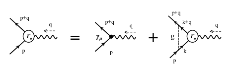
Figure 1: Diagrammatic formalism for the vertex function $\Gamma_{\mu}$. On the right-hand side of the equation, the first diagram corresponds to the bare vertex function (i.e., four-vector current); the second one denotes the vertex correction from the pairing potential.

II.3 Charge conservation

In this part, facilitating with the complete Fock term, we prove the charge conservation from the GIKE. Specifically, we first transform Eq. (5) via a unitary transformation $\rho_{\bf k}(R)={e^{-i\tau_{3}\theta(R)/2}}\rho^{c}_{\bf k}(R)e^{i\tau_{3}\theta(R)/2}$ and obtain

$$\partial_{T}\rho_{\bf k}\!+\!i\left[\left(\xi_{k}\!+\!\mu_{\rm eff}\right)\tau_{3}\!+\!|\Delta|\tau_{1},\rho_{\bf k}\right]\!-\!\Big{[}\frac{i}{8m}\tau_{3},\nabla^{2}_{\bf R}\rho_{\bf k}\Big{]}$$

$$\mbox{}\!-\!\frac{i}{8}\left[({\bm{\nabla}}_{\bf R}\!+\!i{\bf p}_{s}\tau_{3})({\bm{\nabla}}_{\bf R}\!+\!i{\bf p}_{s}\tau_{3})|\Delta|\tau_{1},\partial_{\bf k}\partial_{\bf k}\rho_{\bf k}\right]$$

$$\mbox{}\!-\!\Big{[}\frac{2{\bf p}_{s}\cdot{\bm{\nabla}}_{\bf R}\!+\!{\bm{\nabla}}_{\bf R}\cdot{\bf p}_{s}}{8m}\tau_{3},\tau_{3}\rho_{\bf k}\Big{]}\!+\!\Big{\{}\frac{\bf k}{2m}\tau_{3},{\bm{\nabla}}_{\bf R}\rho_{\bf k}\Big{\}}$$

$$\mbox{}\!+\!\frac{1}{2}\left\{e{\bf E}\tau_{3}\!-\!({\bm{\nabla}}_{\bf R}\!+\!i{\bf p}_{s}\tau_{3})|\Delta|\tau_{1},\partial_{\bf k}\rho_{\bf k}\right\}\!=\!\partial_{t}\rho_{\bf k}\Big{|}_{\rm sc},$$ (12)

with the gauge-invariant measurable superconducting momentum ${\bf p}_{s}$ and effective field $\mu_{\rm eff}$ written as

$${\bf p}_{s} = \nabla_{\bf R}\theta-2e{\bf A},$$ (13)

$$\mu_{\rm eff} = \frac{\partial_{T}\theta}{2}+e\phi+\mu_{H}+\mu_{F}+\frac{p^{2}_{s}}{8m}.$$ (14)

By expanding the density matrix as $\rho_{\bf k}=\sum^{4}_{i=0}\rho_{{\bf k}i}\tau_{i}$, each component of the Fock energy [Eq. (7)] after the unitary transformation $({\hat{\Sigma}_{F}}=g\sum_{\bf k}^{\prime}\tau_{3}\rho_{\bf k}\tau_{3}=\mu_{0}\tau_{0}+\mu_{F}\tau_{3}+|\Delta|\tau_{1})$ reads:

$$g{\sum_{\bf k}}^{\prime}\rho_{{\bf k}3} = \mu_{F},$$ (15)

$$g{\sum_{\bf k}}^{\prime}\rho_{{\bf k}1} = -|\Delta|,$$ (16)

$$g{\sum_{\bf k}}^{\prime}\rho_{{\bf k}2} = 0.$$ (17)

It is noted that Eq. (16) gives the gap equation, from which one can self-consistently obtain the Higgs mode. We show in the following section that from Eq. (17), the NG mode, which has been overlooked in our previous works,GOBE1 ; GOBE2 ; GOBE3 ; GOBE4 can be self-consistently determined.

The gauge-invariant charge density $en$ and current ${\bf j}$ read:GOBE4

$$en = e\sum_{\bf k}\left[1+{\rm Tr}(\rho^{c}_{\bf k}\tau_{3})\right]=e\sum_{\bf k}\left(1+2\rho_{{\bf k}3}\right),$$ (18)

$${\bf j} = \sum_{\bf k}{\rm Tr}\left(\frac{e{\bf k}}{m}\rho^{c}_{\bf k}\right)=2\sum_{\bf k}\left(\frac{e{\bf k}}{m}\rho_{{\bf k}0}\right).~{}~{}~{}$$ (19)

Then, from the $\tau_{3}$ component of the GIKE [Eq. (12)]:

$$\partial_{T}\rho_{{\bf k}3}\!+\!\frac{{\bf k}\cdot{\bm{\nabla}}_{\bf R}\rho_{{\bf k}0}}{m}\!-\!2|\Delta|\rho_{{\bf k}2}\!=\!-(e{\bf E}\cdot{\partial}_{\bf k})\rho_{{\bf k}0}\!-\!\frac{1}{4}$$

$$\mbox{}\!\times\!\{\partial_{\bf k}\partial_{\bf k}\!:\![\rho_{{\bf k}2}({\bm{\nabla}}_{\bf R}{\bm{\nabla}}_{\bf R}\!-\!{\bf p}_{s}{\bf p}_{s})|\Delta|\!-\!\rho_{{\bf k}1}\{{\bm{\nabla}}_{\bf R},{\bf p}_{s}\}|\Delta|]\},$$

(20)

considering the fact that the right-hand side of Eq. (20) vanishes after the summation of ${\bf k}$, one has

$$\partial_{T}\big{(}\sum_{\bf k}\rho_{{\bf k}3}\big{)}+{\bm{\nabla}}_{\bf R}\cdot\big{(}\sum_{\bf k}\frac{{\bf k}}{m}\rho_{{\bf k}0}\big{)}=2|\Delta|{\sum_{\bf k}}^{\prime}\rho_{{\bf k}2},~{}~{}$$ (21)

in which we have used the fact that the gap vanishes outside the spherical shell in the BCS theory,G1 ; BCS $\sum_{\bf k}|\Delta|\rho_{{\bf k}2}={\sum_{\bf k}}^{\prime}|\Delta|\rho_{{\bf k}2}$. Consequently, since the right-hand side of Eq. (21) is zero because of Eq. (17), by looking into the charge density [Eq. (18)] and current [Eq. (19)] expressions, one immediately obtains the charge conservation:

$$\partial_{T}en+{\bm{\nabla}}_{\bf R}\cdot{\bf j}=0.$$ (22)

Therefore, in the GIKE approach, the charge conservation is naturally satisfied with the complete Foch term [Eqs. (16) and (17)], in contrast to the Ambegaokar and Kadanoff’s approachAK where an additional condition of the charge conservation is required to obtain NG mode. This is because that the Fock energy in the GIKE is equivalent to the generalized Ward’s identity by Nambu,gi0 ; Ba0 as proved in Sec. II.2.1, and hence, the gauge invariance in the GIKE directly leads to the charge conservation.

III Analytic Analysis

In this section, we perform the analytical analysis for the electromagnetic response of the collective Higgs and NG modes in the linear and second-order regimes. By assuming the external electromagnetic potential $\phi=\phi_{0}(\omega,{\bf q})e^{i\omega{t}-i{\bf q}\cdot{\bf R}}$ and ${\bf A}={\bf A}_{0}(\omega,{\bf q})e^{i\omega{t}-i{\bf q}\cdot{\bf R}}$, the density matrix $\rho_{\bf k}$ and charge density $en$ read:

$$\rho_{\bf k} = \rho^{0}_{\bf k}+\rho^{\omega}_{\bf k}e^{i\omega{t}-i{\bf q}\cdot{\bf R}}+\rho^{2\omega}_{\bf k}e^{2i\omega{t}-2i{\bf q}\cdot{\bf R}},$$ (23)

$$en = en_{0}+en^{\omega}e^{i\omega{t}-i{\bf q}\cdot{\bf R}}+en^{2\omega}e^{2i\omega{t}-2i{\bf q}\cdot{\bf R}},$$ (24)

whereas the phase $\theta$ and amplitude $|\Delta|$ of the order parameter are written as

$$\theta = \theta^{\omega}e^{i\omega{t}-i{\bf q}\cdot{\bf R}}+\theta^{2\omega}e^{2i\omega{t}-2i{\bf q}\cdot{\bf R}},$$ (25)

$$|\Delta| = \Delta_{0}+\delta|\Delta|^{\omega}e^{i\omega{t}-i{\bf q}\cdot{\bf R}}+\delta|\Delta|^{2\omega}e^{2i\omega{t}-2i{\bf q}\cdot{\bf R}}.~{}~{}~{}~{}$$ (26)

Here, $\rho^{0}_{\bf k}$, $en_{0}$ and $\Delta_{0}$ are the density matrix, charge density and order parameter in equilibrium state, respectively; $\rho^{\omega(2\omega)}_{\bf k}$, $en^{\omega(2\omega)}$, $\theta^{\omega(2\omega)}$ and $\delta|\Delta|^{\omega(2\omega)}$ denote the linear (second-order) responses of the density matrix, charge density, Higgs mode and NG mode, respectively.

The density matrix in equilibrium state is given byGOBE1 ; GOBE4

$$\rho^{0}_{\bf k}=\frac{1}{2}-\frac{f_{k}}{2}\left(\frac{\xi_{k}}{E_{k}}\tau_{3}+\frac{\Delta_{0}}{E_{k}}\tau_{1}\right)$$ (27)

with $f_{k}=1-2n_{F}(E_{k})$ and $E_{k}=\sqrt{\xi_{k}^{2}+\Delta_{0}^{2}}$. Here, $n_{F}(x)$ is the Fermi-distribution function. From Eq. (16), $\Delta_{0}$ is determined by

$$\Delta_{0}=-g{\sum_{\bf k}}^{\prime}\rho^{0}_{{\bf k}1}=g{\sum_{\bf k}}^{\prime}\left(\frac{\Delta_{0}}{2E_{k}}f_{k}\right),$$ (28)

which is exactly the gap equation in the BCS theory.BCS $en_{0}$ from Eq. (18) is written as

$$en_{0}=e\sum_{\bf k}(1+2\rho^{0}_{{\bf k}3})=\sum_{\bf k}\Big{[}2ev^{2}_{k}+2e\frac{\xi_{k}}{E_{k}}n_{F}(E_{k})\Big{]},$$ (29)

consisting of the charge densities of the condensatecn0 ; cn1 ; cn2 ; cn3 $2ev^{2}_{k}=e(1-\frac{\xi_{k}}{E_{k}})$ and Bogoliubov quasiparticlescn0 ; cn1 ; cn2 ; cn3 ; cn4 ; cn5 $2e\frac{\xi_{k}}{E_{k}}n_{F}(E_{k})$.

Then, we show that the GIKE [Eq. (12)] provides an efficient approach to study the electromagnetic responses of the collective NG and Higgs modes.

III.1 Linear response

We first focus on the linear response in this part. From Eqs. (13) and (14), the linear responses of the superconducting momentum ${\bf p}_{s}^{\omega}$ and effective field $\mu_{\rm eff}^{\omega}$ are given by

$${\bf p}^{\omega}_{s} = -i{\bf q}\theta^{\omega}-2e{\bf A}_{0},$$ (30)

$$\mu^{\omega}_{\rm eff} = \frac{i\omega\theta^{\omega}}{2}+e\phi_{0}+\mu^{\omega}_{H}+\mu^{\omega}_{F}.$$ (31)

with the linear responses of the Hartree field $\mu^{\omega}_{H}$ [Eq. (6)] and Fock one $\mu^{\omega}_{F}$ [Eq. (15)] written as

$$\mu^{\omega}_{H} = V_{q}n^{\omega}=2V_{q}\sum_{\bf k}\rho^{\omega}_{{\bf k}3},$$ (32)

$$\mu^{\omega}_{F} = g\sum_{\bf k}\rho^{\omega}_{{\bf k}3}.$$ (33)

We then investigate the linear responses of the NG mode $\theta^{\omega}$ and Higgs mode $\delta|\Delta|^{\omega}$.

III.1.1 NG mode

We address the NG mode in this part. In the long-wave limit, we only keep the lowest two orders of ${\bf q}$. In this situation, the linear response of the density matrix $\rho^{\omega}_{\bf k}$ can be solved from the GIKE. Substituting the linear solution of $\rho^{\omega}_{{\bf k}2}$ into Eq. (17), one has (refer to Appendix A)

$$i\omega\mu^{\omega}_{\rm eff}\left(1+\frac{q^{2}v^{2}_{F}}{3\omega^{2}}g_{\omega}\right)+\frac{i{\bf q}\cdot{\bf p}_{s}^{\omega}}{2}\frac{v_{F}^{2}}{3}s_{\omega}=i\omega\delta|\Delta|^{\omega}b_{\omega},$$ (34)

with the dimensionless factors:

$$s_{\omega} = \frac{{\sum_{\bf k}}^{\prime}\Big{[}\frac{1}{4E_{k}^{2}-\omega^{2}}\big{(}2-{E_{k}^{2}\partial^{2}_{\xi_{k}}}\big{)}\big{(}\frac{\Delta_{0}}{2E_{k}}f_{k}\big{)}\Big{]}}{{\sum_{\bf k}}^{\prime}\big{(}\frac{1}{4E_{k}^{2}-\omega^{2}}\frac{\Delta_{0}}{E_{k}}f_{k}\big{)}},$$ (35)

$$g_{\omega} = \frac{{\sum_{\bf k}}^{\prime}\Big{[}\frac{\Delta_{0}}{4E_{k}^{2}-\omega^{2}}\partial_{\xi_{k}}\big{(}\frac{\xi_{k}}{E_{k}}f_{k}\big{)}\Big{]}}{{\sum_{\bf k}}^{\prime}\big{(}\frac{1}{4E_{k}^{2}-\omega^{2}}\frac{\Delta_{0}}{E_{k}}f_{k}\big{)}},$$ (36)

$$b_{\omega} = \frac{{\sum_{\bf k}}^{\prime}\big{(}\frac{1}{4E_{k}^{2}-\omega^{2}}\frac{\xi_{k}}{E_{k}}f_{k}\big{)}}{{\sum_{\bf k}}^{\prime}\big{(}\frac{1}{4E_{k}^{2}-\omega^{2}}\frac{\Delta_{0}}{E_{k}}f_{k}\big{)}}=0.$$ (37)

Here, we have taken care of the particle-hole symmetry to remove terms with the odd order of $\xi_{k}$ in the summation of ${\bf k}$. Consequently, since $b_{\omega}=0$ [Eq. (37)], it is obvious that the linear response of the NG mode decouples with that of the Higgs mode ($\delta|\Delta|^{\omega}$) due to the particle-hole symmetry, in consistency with the symmetry analysis.symmetry

Further substituting ${\bf p}_{s}^{\omega}$ [Eq. (30)] and $\mu^{\omega}_{\rm eff}$ [Eq. (31)] into Eq. (34), one obtains the linear-response equation of the NG mode:

$$\Big{[}\omega^{2}-\frac{q^{2}v_{F}^{2}}{3}(s_{\omega}-g_{\omega})\Big{]}\frac{\theta^{\omega}}{2}=i\omega{e\phi_{0}}-\frac{v^{2}_{F}}{3}s_{\omega}i{\bf q}\cdot{e{\bf A}_{0}}-\frac{q^{2}v^{2}_{F}}{3}g_{\omega}\frac{e\phi_{0}}{i\omega}+i\omega(\mu^{\omega}_{H}+\mu^{\omega}_{F})\Big{(}1+\frac{q^{2}v^{2}_{F}}{3\omega^{2}}g_{\omega}\Big{)}.$$ (38)

We first discuss the situation without the Hartree and Fock terms. In the low-frequency regime with $\omega\ll 2\Delta_{0}$, one finds $s_{\omega}\approx 1$ and $g_{\omega}\approx 2/3$ (refer to Appendix A). Hence, the linear-response equation of the NG mode [Eq. (38)] becomes

$$\Big{[}\omega^{2}-\Big{(}\frac{qv_{F}}{3}\Big{)}^{2}\Big{]}\frac{\theta^{\omega}}{2}=i\omega{e\phi_{0}}\Big{[}1+2\Big{(}\frac{qv_{F}}{3\omega}\Big{)}^{2}\Big{]}-\frac{v^{2}_{F}}{3}i{\bf q}\cdot{e{\bf A}_{0}}.$$ (39)

Consequently, it is found that the collective NG mode exhibits the gapless linear energy spectrum (i.e., $\omega_{\rm NG}={qv_{F}}/{3}$) inside the superconducting gap, in consistency with the previous worksgi0 ; AK ; Ba0 ; pm0 ; Am0 ; pi1 ; Ba9 ; Ba10 ; gi1 ; pm5 and Goldstone theorem with the spontaneous continuous $U(1)$-symmetry breaking.Gm1 ; Gm2 Additionally, the NG mode responds to the longitudinal electromagnetic field [right-hand side of Eq. (39)] in the linear regime, also in agreement with the previous works.AK ; Ba0 ; Ba9 ; Ba10

III.1.2 Role of Hartree and Fock fields

We next consider the role of the Hartree and Fock fields in the linear response of the NG mode. Specifically, considering $V_{q}\gg{g}$ in the long-wave limit, the Fock field can be neglected. Substituting the solution of $\rho^{\omega}_{{\bf k}3}$ into Eq. (32), the Hartree field reads (refer to Appendix B):

$$\mu^{\omega}_{H}=\frac{V_{q}{\bf q}\cdot{\bf E}^{\omega}}{im\omega^{2}}{\sum_{\bf k}}^{\prime}\frac{k_{F}^{2}}{3m}\Big{[}{\partial_{E_{k}}f_{k}}-\frac{\Delta^{2}_{0}}{E_{k}}\partial_{E_{k}}\Big{(}\frac{f_{k}}{E_{k}}\Big{)}\Big{]}.$$ (40)

It is noted that the first term in the summation of ${\bf k}$ denotes the contribution from the Bogoliubov quasiparticles. The second one exactly corresponds to the Meissner-superfluid density $\rho_{s}=\sum_{\bf k}^{\prime}\frac{k_{F}^{2}}{3m}\big{[}\frac{\Delta^{2}_{0}}{E_{k}}\partial_{E_{k}}\big{(}-\frac{f_{k}}{E_{k}}\big{)}\big{]}$, related to the Meissner supercurrent, as revealed in our previous work.GOBE4

At low temperature, the Bogoliubov quasiparticles vanish, i.e., $n_{F}(E_{k})\approx 0$, leaving solely the Meissner-superfluid density. Then, one has $\mu^{\omega}_{H}=-\frac{i{\bf q}\cdot{e}{\bf E}^{\omega}}{{q^{2}}}\frac{\omega^{2}_{p}}{\omega^{2}}$ with $\omega_{p}=\sqrt{\frac{\rho_{s}e^{2}}{\epsilon_{0}m}}$ being the plasma frequency. Further substituting ${\bf E}^{\omega}$ [Eq. (8)] into $\mu^{\omega}_{H}$, the Hartree field is given by

$$\mu^{\omega}_{H}=-\frac{i{\bf q}{\cdot}e{\bf E}^{\omega}_{0}}{q^{2}}\frac{\omega^{2}_{p}/\omega^{2}}{1-{\omega^{2}_{p}}/{\omega^{2}}},$$ (41)

with $e{\bf E}_{0}=i{\bf q}\phi_{0}-i\omega{\bf A}_{0}$ being the external electric field.

Finally, considering the contribution of the Hartree field [Eq. (41)], the linear-response equation [Eq. (38)] of the NG mode becomes

$$\Big{[}\omega^{2}-\Big{(}\frac{qv_{F}}{3}\Big{)}^{2}\Big{]}\frac{\theta^{\omega}}{2}=\frac{i\omega{e\phi_{0}-\omega^{2}_{p}{i{\bf q}{\cdot}e{\bf A}_{0}}/{q^{2}}}}{1-\omega^{2}_{p}/\omega^{2}}+O(q).~{}~{}$$ (42)

Therefore, as seen from the right-hand side of Eq. (42), as a consequence of the Hartree field (i.e., the vacuum polarization), the longitudinal field experiences the Coulomb screening. In this situation, multiplying by $1-\omega^{2}_{p}/\omega^{2}$ on both sides of Eq. (42), in the long-wave limit, one has

$$(\omega^{2}-\omega_{p}^{2})\frac{\theta^{\omega}}{2}=i\omega{e\phi_{0}}-\omega^{2}_{p}\frac{i{\bf q}{\cdot}e{\bf A}_{0}}{q^{2}},$$ (43)

exactly same as the previous work.AK Consequently, as seen from Eq. (43), the linear response of the NG mode interacts with the long-range Coulomb interaction, causing the original gapless spectrum of the NG mode effectively lifted up to the high-energy plasma frequency as a result of the Anderson-Higgs mechanism.AK ; Ba0 ; pm0 ; pm5 ; Am0 ; AHM

With the high-energy plasma frequency (i.e., $\omega\ll\omega_{p}$), one finds ${\theta^{\omega}}/{2}={i{\bf q}{\cdot}e{\bf A}_{0}}/{q^{2}}$. As pointed out in the previous works,Ba0 ; AK this finite $\theta^{\omega}$ from the unphysical longitudinal vector potential does not provide any measurable effect, especially considering the fact that the longitudinal vector potential does not even exist in either optical response or static magnetic response. Moreover, this finite $\theta^{\omega}$ cancels the unphysical longitudinal vector potential in ${\bf p}^{\omega}_{s}$ [Eq. (30)]:

$$\frac{{\bf p}^{\omega}_{s}}{2}=\frac{{\bf q}({\bf q}{\cdot}e{\bf A}_{0})}{q^{2}}-e{\bf A}_{0}+O\Big{(}\frac{\omega^{2}}{\omega^{2}_{p}}\Big{)}.$$ (44)

As a result, the gauge-invariant superconducting momentum ${\bf p}^{\omega}_{s}$, which appears in the Ginzburg-Landau equation,G1 ; GOBE4 Meissner supercurrentG1 ; GOBE4 and Anderson-pump effect,Am1 ; Am2 ; Am7 ; Am9 ; Am11 ; Am14 ; NL7 ; NL8 ; NL9 ; NL10 ; NL11 ; Am3 ; Am4 ; Am8 ; Am10 ; GOBE1 ; GOBE2 ; GOBE3 ; GOBE4 only involves the physical transverse vector potential.

Interestingly, at low temperature, it is observed above that the emerged plasma frequency $\omega_{p}=\sqrt{\frac{\rho_{s}e^{2}}{\epsilon_{0}m}}$ origins from the Meissner-superfluid density $\rho_{s}=\sum_{\bf k}^{\prime}\frac{k_{F}^{2}}{3m}\frac{\Delta_{0}^{2}}{E^{3}_{k}}$, rather than the condensate $en_{0}=\sum_{\bf k}2ev_{k}^{2}$. This is in consistency with our previous conclusionGOBE4 that only the Meissner-superfluid density, which is related to the charge fluctuation on top of the condensate, is involved in the electromagnetic response in the superconducting states whereas the ground state condensate simply provides a rigid background.

III.1.3 Higgs mode

We next study the linear response of the Higgs mode. Substituting the second-order solution of $\rho^{\omega}_{{\bf k}1}$ into the gap equation [Eq. (16)], one directly obtains (refer to Appendix A)

$${i\omega\delta|\Delta|^{\omega}}\Big{[}\frac{1}{g}-{\sum_{\bf k}}^{\prime}\Big{(}\frac{2\xi^{2}_{k}}{4E^{2}_{k}-\omega^{2}}\frac{f_{k}}{E_{k}}\Big{)}\Big{]}=-\frac{i({\bf q}\cdot{\bf p}^{\omega}_{s})c_{\omega}}{6m}$$

$$\mbox{}+\frac{i{\bf q}}{m}\cdot\frac{e{\bf E}^{\omega}}{i\omega}{\sum_{\bf k}}^{\prime}\Big{[}\frac{4\xi^{2}_{k}}{4E^{2}_{k}-\omega^{2}}\frac{2}{3}\partial_{\xi_{k}}(\xi_{k}\rho^{0}_{{\bf k}1})\Big{]},$$ (45)

where the particle-hole symmetry has been taken care of to remove terms with odd order of $\xi_{k}$ in the summation of ${\bf k}$. $c_{\omega}$ is a dimensionless factor (refer to Appendix A).

The first term on the right-hand side of Eq. (45) vanishes since ${\bf p}^{\omega}_{s}$ only involves the physical transverse vector potential [Eq. (44)]. By using Eq. (28) to replace $g$, the linear response of the Higgs mode is obtained:

$$i\omega\delta|\Delta|^{\omega}\Big{[}1-\Big{(}\frac{\omega}{2\Delta_{0}}\Big{)}^{2}\Big{]}=u_{\omega}\frac{i{\bf q}{\cdot}e{\bf E}^{\omega}}{im\omega},$$ (46)

with $u_{\omega}={{\sum_{\bf k}}^{\prime}\Big{[}\frac{4\xi^{2}_{k}\partial_{\xi_{k}}(\xi_{k}\rho^{0}_{{\bf k}1})}{4E^{2}_{k}-\omega^{2}}\Big{]}}/{{\sum_{\bf k}}^{\prime}\Big{(}\frac{3\Delta_{0}^{2}}{4E^{2}_{k}-\omega^{2}}\frac{f_{k}}{E_{k}}\Big{)}}$.

Consequently, from Eq. (46), it is seen that the Higgs mode exhibits the gapful energy spectrum (i.e., $\omega_{\rm H}=2\Delta_{0}$), in consistency with the previous studies.Am0 ; pm5 Moreover, the Higgs mode also responds to the electromagnetic field in the linear regime [right-hand side of Eq. (46)]. Nevertheless, this linear response vanishes in the long-wave limit, making it hard to be detected in the optical experiment.

III.2 Second-order response

From above analytic investigations, one directly concludes that neither the collective phase (NG) mode nor the amplitude (Higgs) mode is detectable in the linear regime for the optical experiment. In contrast, we show in this section that the second-order response of the collective modes in superconductors exhibits different physics.

Specifically, the second-order responses of the superconducting momentum ${\bf p}_{s}^{2\omega}$ and effective field $\mu_{\rm eff}^{2\omega}$ from Eqs. (13) and (14) are given by

$${\bf p}^{2\omega}_{s} = -2i{\bf q}\theta^{2\omega},$$ (47)

$$\mu^{2\omega}_{\rm eff} = i\omega\theta^{2\omega}+\mu^{2\omega}_{H}+\mu^{2\omega}_{F}+\frac{(p^{\omega}_{s})^{2}}{8m}.$$ (48)

It is noted that the last term on the right-hand side of Eq. (48) is exactly the Anderson-pump effect.

The second-order responses of the Hartree field $\mu^{2\omega}_{H}$ [Eq. (6)] and Fock one $\mu^{2\omega}_{F}$ [Eq. (15)] are written as

$$\mu^{2\omega}_{H} = V_{2q}n^{2\omega}=2V_{2q}\sum_{\bf k}\rho^{2\omega}_{{\bf k}3},$$ (49)

$$\mu^{2\omega}_{F} = g\sum_{\bf k}\rho^{2\omega}_{{\bf k}3}.$$ (50)

Then, we investigate the second-order responses of the NG mode $\theta^{2\omega}$ and Higgs mode $\delta|\Delta|^{2\omega}$.

III.2.1 NG mode

We address the NG mode in this part. The second-order response of the density matrix $\rho^{2\omega}_{\bf k}$ can also be obtained from the GIKE in the long-wave limit. Substituting the solution of $\rho^{2\omega}_{{\bf k}2}$ into Eq. (17), one has (refer to Appendix C)

$$2i\omega\mu^{2\omega}_{\rm eff}\Big{(}1+\frac{q^{2}v^{2}_{F}}{3\omega^{2}}g_{2\omega}\Big{)}+{i{\bf q}\cdot{\bf p}_{s}^{2\omega}}\frac{v^{2}_{F}}{3}s_{2\omega}=\frac{2i\omega}{m}\Big{[}\frac{g_{2\omega}}{3}$$

$$\mbox{}\times\Big{(}\frac{e{\bf E}^{\omega}}{i\omega}-{{\bf p}^{\omega}_{s}}\Big{)}{\cdot}\frac{e{\bf E}^{\omega}}{i\omega}+\frac{l_{\omega}}{2}\Big{(}\frac{e{\bf E}^{\omega}}{i\omega}-\frac{{\bf p}^{\omega}_{s}}{2}\Big{)}^{2}\Big{]},~{}~{}~{}~{}~{}~{}$$ (51)

with dimensionless prefactor:

$$l_{\omega}=\frac{{\sum_{\bf k}}^{\prime}\Big{[}\frac{\Delta_{0}}{E_{k}^{2}-\omega^{2}}(2\xi_{k}\partial^{2}_{\xi_{k}}+\partial_{\xi_{k}})\Big{(}\frac{\xi_{k}}{E_{k}}f_{k}\Big{)}\Big{]}}{3{\sum_{\bf k}}^{\prime}\Big{(}\frac{1}{E_{k}^{2}-\omega^{2}}\frac{\Delta_{0}}{E_{k}}f_{k}\Big{)}}.$$ (52)

Furthermore, with the solution of $\rho^{2\omega}_{{\bf k}3}$, we find that the second-order response of the charge density $en^{2\omega}=e\sum_{\bf k}2\rho^{2\omega}_{{\bf k}3}$ is zero (refer to Appendix C), leading to the vanishing second-order Hartree field $\mu^{2\omega}_{H}$ [Eq. (49)] and Fock one $\mu^{2\omega}_{F}$ [Eq. (50)].

Consequently, substituting ${\bf p}_{s}^{2\omega}$ [Eq. (47)] and $\mu^{2\omega}_{\rm eff}$ [Eq. (48)] into Eq. (51), the second-order response equation of the NG mode reads:

$$\Big{[}\omega^{2}-\frac{q^{2}v_{F}^{2}}{3}(s_{2\omega}-g_{2\omega})\Big{]}\theta^{2\omega}=\frac{i\omega}{m}\Big{[}\frac{({\bf p}_{s}^{\omega})^{2}}{8}-\frac{g_{2\omega}}{3}$$

$$\mbox{}\times\Big{(}\frac{e{\bf E}^{\omega}}{i\omega}-{{\bf p}^{\omega}_{s}}\Big{)}{\cdot}\frac{e{\bf E}^{\omega}}{i\omega}-\frac{l_{\omega}}{2}\Big{(}\frac{e{\bf E}^{\omega}}{i\omega}-\frac{{\bf p}^{\omega}_{s}}{2}\Big{)}^{2}\Big{]},~{}~{}~{}~{}~{}~{}$$ (53)

which exhibits different physics from the linear response.

Particularly, in the low-frequency regime ($\omega\ll{\Delta_{0}}$), one finds that $s_{2\omega}\approx 1/3$, $g_{2\omega}\approx 2/3$, (refer to Appendix A) and $l_{\omega}\approx-2/45$ (refer to Appendix C), and hence, Eq. (53) becomes

$$\Big{(}\omega^{2}-\frac{q^{2}v_{F}^{2}}{9}\Big{)}{\theta^{2\omega}}\approx\frac{i\omega}{m}\frac{({\bf p}_{s}^{\omega})^{2}}{8}+\Big{(}{{\bf p}^{\omega}_{s}}-\frac{e{\bf E}^{\omega}}{i\omega}\Big{)}{\cdot}\frac{e{\bf E}^{\omega}}{5m}.$$ (54)

On the right-hand side of Eq. (54), the first term exactly comes from the Anderson pump effect whereas the last two ones are attributed to the second order of the drive effect. Both effects play important role in the second-order response of the NG mode. Moreover, it is noted that on the right-hand side of in Eq. (53), ${\bf p}^{\omega}_{s}$ only involves the physical transverse vector potential [Eq. (44)]. As for the electric field ${\bf E}^{\omega}={\bf E}^{\omega,\parallel}+{\bf E}^{\omega,\perp}$, by the linear response of the Hartree field $\mu^{\omega}_{H}$ (i.e., the vacuum polarization), the longitudinal electric field ${\bf E}^{\omega,\parallel}$ is suppressed by the strong Coulomb screening whereas the transverse one ${\bf E}^{\omega,\perp}$ is not affected (refer to Appendix B). Therefore, the second-order response of the NG mode at low frequency ($\omega{\ll}\omega_{p}$) is determined by the transverse field.

Consequently, from Eq. (54), it is very interesting to find that due to the vanishing Hartree field, the second-order response of the NG mode maintains the original gapless energy spectrum ($\omega_{\rm NG}=qv_{F}/3$) inside the superconducting gap, in striking contrast to the linear response with the Anderson-Higgs mechanism. This can be understood as follows. In the presence of the inverse symmetry, no second-order current is induced, and hence, due to the charge conservation, no charge density fluctuation $en^{2\omega}$ is excited, effectively ruling out the Hartree field $\mu^{2\omega}_{H}=V_{q}n^{2\omega}$ (i.e., the long-range Coulomb interaction) in the second-order response. In addition, differing from the linear response excited by the longitudinal field solely, the second-order response of the NG mode is determined by the transverse field as mentioned above, free from the influence of the Coulomb screening.

We point out that thanks to the gauge-invariant electric field and superconducting moment on the right-hand side of Eq. (54), the second-order response of the NG mode $\theta^{2\omega}$ is a measurable quantity, differing from the linear response above. This term, which is hard to deal with in the previous approaches,AK ; Ba0 ; Ba9 ; Ba10 ; pm0 ; pm5 ; Am0 ; pi1 ; pi4 has long been overlooked in the literature.

III.2.2 Higgs mode

Substituting the solution of $\rho^{2\omega}_{{\bf k}1}$ into Eq. (16), in the long-wave limit, one has (refer to Appendix C)

$$\frac{\delta|\Delta|^{2\omega}}{g}\!=\!{\sum_{\bf k}}^{\prime}\frac{\xi_{k}\Big{[}\delta|\Delta|^{2\omega}+\big{(}\frac{{\bf p}^{\omega}_{s}}{2}-\frac{e{\bf E}^{\omega}}{i\omega}\big{)}^{2}\frac{\Delta_{0}v^{2}_{F}\partial^{2}_{\xi_{k}}}{6}\Big{]}\rho^{0}_{{\bf k}3}}{\omega^{2}-E^{2}_{k}}.~{}~{}$$ (55)

By using Eq. (28) to replace $g$, the second-order response equation of the Higgs mode in the long-wave limit reads:

$$\delta|\Delta|^{2\omega}\Big{[}1-\Big{(}\frac{2\omega}{2\Delta_{0}}\Big{)}^{2}\Big{]}=\frac{v_{F}^{2}}{6}\Big{(}\frac{{\bf p}^{\omega}_{s}}{2}-\frac{e{\bf E}^{\omega}}{i\omega}\Big{)}^{2}\frac{d_{\omega}}{\Delta_{0}},$$ (56)

with $d_{\omega}={{\sum_{\bf k}}^{\prime}\Big{[}\frac{\xi_{k}\Delta_{0}}{E_{k}^{2}-\omega^{2}}\partial^{2}_{\xi_{k}}\Big{(}\frac{\xi_{k}}{E_{k}}f_{k}\Big{)}\Big{]}}/{{\sum_{\bf k}}^{\prime}\Big{(}\frac{f_{k}}{E_{k}}\frac{\Delta_{0}}{E_{k}^{2}-\omega^{2}}\Big{)}}$.

Therefore, a finite response of the Higgs mode in the long-wave limit is found in the second-order regime, differing from the vanishing linear response above. Furthermore, this second-order response of the Higgs mode, shows a resonance at $2\omega=2\Delta_{0}$, in consistency with the experimental findings.NL8 ; NL9 ; NL10 Particularly, we point out that the right-hand side of Eq. (56) exactly comes from the second-order of drive effect whereas the widely considered pump effect in the literatureAm1 ; Am2 ; Am7 ; Am9 ; Am11 ; Am14 ; NL7 ; NL8 ; NL9 ; NL10 ; NL11 ; Am3 ; Am4 ; Am8 ; Am10 ; GOBE1 ; GOBE2 ; GOBE3 ; GOBE4 makes no contribution at all.

Actually, it is noted that in the previous theoretical studies,Am1 ; Am2 ; Am3 ; Am4 ; Am5 ; Am6 ; Am7 ; Am8 ; Am9 ; Am10 ; Am11 ; Am12 ; Am13 ; Am14 ; NL7 ; NL8 ; NL9 ; NL10 ; NL11 ; GOBE1 ; GOBE2 ; GOBE3 ; GOBE4 the obtained fluctuation of the order parameter $\delta\Delta^{2\omega}$ is directly considered as the amplitude (Higgs) mode $\delta|\Delta|^{2\omega}$ since it is believed that the phase (NG) mode is lifted up to the high-energy plasma frequency. Then, it is considered that the Anderson-pump effect, which can excite the fluctuation of the order parameter $\delta\Delta^{2\omega}$, contributes to the amplitude mode. Nevertheless, this becomes ambiguous when the very recent symmetry analysis by Tsuchiya et al.symmetry implies that the pump effect excites the oscillation of the superconducting phase rather than the amplitude. Even though not clearly stated, the obtained pseudospin susceptibilities $\chi_{yz}\neq 0$ and $\chi_{xz}=0$ [Eq. (25) in Ref. symmetry, ] in their work clearly suggest that the induced pseudo field $H_{z}$ by the pump effect in the Anderson pseudospin pictureAm1 ; Am2 ; Am7 ; Am9 ; Am11 ; Am14 ; NL7 ; NL8 ; NL9 ; NL10 ; NL11 can only generate the fluctuation of the phase-related $S_{y}$, rather than the amplitude-related $S_{x}$. To resolve this puzzle, the contributions from the amplitude and phase modes to $\delta\Delta^{2\omega}$ in the previous worksAm1 ; Am2 ; Am3 ; Am4 ; Am5 ; Am6 ; Am7 ; Am8 ; Am9 ; Am10 ; Am11 ; Am12 ; Am13 ; Am14 ; NL7 ; NL8 ; NL9 ; NL10 ; NL11 ; GOBE1 ; GOBE2 ; GOBE3 ; GOBE4 must be carefully examined.

In contrast, the GIKE provides an efficient approach to calculate the phase and amplitude modes on an equal footing. The results from the GIKE above suggest that the fluctuation of the order parameter in the second-order response actually consists of contributions from both amplitude (Higgs) and phase (NG) modes, i.e., $\delta\Delta^{2\omega}=\delta|\Delta|^{2\omega}+i\theta^{2\omega}\Delta_{0}$. From above analytic analysis, we conclude that the observed second-order response of the amplitude mode $\delta|\Delta|^{2\omega}$ in the recent optical experimentsNL7 ; NL8 ; NL9 ; NL10 ; NL11 is attributed solely to the drive effect rather than the widely considered Anderson-pump effect.Am1 ; Am2 ; Am7 ; Am9 ; Am11 ; Am14 ; NL7 ; NL8 ; NL9 ; NL10 ; NL11 ; Am3 ; Am4 ; Am8 ; Am10 ; GOBE1 ; GOBE2 ; GOBE3 ; GOBE4

In fact, the pump effect only contributes to the second-order response of the NG mode $\theta^{2\omega}$, in which the drive effect also plays an important role, as mentioned in Sec. III.2.1. Consequently, all previous studies of the Anderson-pump effect in the literatureAm1 ; Am2 ; Am3 ; Am4 ; Am5 ; Am6 ; Am7 ; Am8 ; Am9 ; Am10 ; Am11 ; Am12 ; Am13 ; Am14 ; NL7 ; NL8 ; NL9 ; NL10 ; NL11 ; GOBE1 ; GOBE2 ; GOBE3 ; GOBE4 actually calculate only one part of the second-order response of the NG mode $\theta^{2\omega}$ rather than the Higgs mode, supporting the latest symmetry analysis by Tsuchiya et al.symmetry from the Anderson pseudospin picture. Particularly, we have revealed in Sec. III.2.1 that the second-order response of the NG mode decouples with the long-range Coulomb interaction, free from the influence of the Anderson-Higgs mechanism,AHM and is measurable. A tentative scheme to detect this second-order response of the NG mode is proposed in the following section.

III.2.3 Tentative scheme for detection

We propose a tentative scheme to detect the second-order response $\theta^{2\omega}$ through the Josephson junction. Specifically, for the optical experiment, in the long-wave limit, the second-order response of the NG mode from Eq. (54) shows a spatially uniform but temporally oscillating phase $\theta=z_{\omega}e^{2i\omega{t}}$, with $z_{\omega}=|\theta^{2\omega}(q=0)|$ denoting the oscillating amplitude of $\theta$. Therefore, as schematically illustrated in Fig. 2, in a Josephson junction, by separately applying two phase-locked continuous-wave optical fields with frequencies $\omega_{L}$ and $\omega_{R}$ ($\omega_{L}=2\omega_{R}$) to the superconductors on each side of junction, an oscillating phase difference $\theta_{d}=\theta_{L}-\theta_{R}$ between the left and right superconductors is induced, leading to the Josephson current $J=J_{c}\sin\theta_{d}$.Josephson Here, $J_{c}$ is the Josephson critical current. Moreover, through the optical time delay to choose $\pi/2$ phase difference, one has the phase excitations with $\theta_{L}=z^{L}_{\omega_{L}}\cos(2\omega_{L}t)$ and $\theta_{R}=z^{R}_{\omega_{R}}\sin(2\omega_{R}t)$, and then, a dc-current component in $J$ is derived (refer Appendix D):

$$J^{\rm dc}\!=\!2J_{c}\!j_{1}(z^{L}_{\omega_{L}})j_{2}(z^{R}_{\omega_{R}}),$$ (57)

with $j_{n}(x)$ being the $n$-th Bessel function of the first kind.

Consequently, a dc current is induced. Therefore, this dc Josephson current provides a tentative scheme for the detection of the second-order response of the NG (phase) mode, especially considering the fact that the generation of the Josephson current directly implies the phase fluctuation. Moreover, to avoid influence from the optical currents, one can choose the directions of the propagation and polarization of the applied optical fields to be perpendicular to that of the junction, i.e., along $z$ and $y$ directions in Fig. 2, respectively.

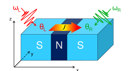
Figure 2: Schematic to detect the second-order response of the phase mode. Two continuous-wave optical fields with frequencies $\omega_{L}$ and $\omega_{R}=\omega_{L}/2$ are applied to the superconductors on the two side of junction, leading to the excited phase $\theta_{L}$ ($\theta_{R}$) of the left (right) superconductor. Then, by the phase difference $\theta_{d}=\theta_{L}-\theta_{R}$, the Josephson current $J=J_{c}\sin\theta_{d}$ is generated.

IV SUMMARY AND DISCUSSION

We have shown that the GIKE provides an efficient approach to study the electromagnetic response of the collective modes in the superconducting states. We prove that the Fock energy is equivalent to the generalized Ward’s identity by Nambu.gi0 ; Ba0 Therefore, with the complete Fock term, the gauge invariance in the GIKE directly leads to the charge conservation, in contrast to the previous Ambegaokar and Kadanoff’s approachAK where an additional condition of the charge conservation is required to obtain the NG mode. Differing from the previous studies in the literature with either the fixed amplitudeAK ; pi1 ; pm1 ; pm2 ; pi4 ; Ba9 or overlooked phaseAm1 ; Am2 ; Am3 ; Am4 ; Am5 ; Am6 ; Am7 ; Am8 ; Am9 ; Am10 ; Am11 ; Am12 ; Am13 ; Am14 ; NL7 ; NL8 ; NL9 ; NL10 ; NL11 ; GOBE1 ; GOBE2 ; GOBE3 ; GOBE4 of the order parameter, in the present work, the gapless NG and gapful Higgs modes are calculated on an equal footing. Moreover, both linear and nonlinear responses are investigated.

In the linear regime, we find that the Higgs mode responds to the electromagnetic field but this linear response vanishes in the long-wave limit. As for the NG mode, the results in the linear response by the GIKE agree with the previous ones in the literature.AK ; Ba0 ; pm0 ; pm5 ; Am0 ; Ba9 ; Ba10 Specifically, the linear response of the NG mode interacts with the long-range Coulomb interaction, causing the original gapless spectrum inside the superconducting gap effectively lifted up to the plasma frequency far above the gap as a result of the Anderson-Higgs mechanism.AHM Consequently, no effective linear response of the NG mode occurs. In addition, we reveal that the emerged plasma frequency at low temperature origins from the Meissner-superfluid density rather than the condensate, in consistency with our previous conclusionGOBE4 that only the Meissner-superfluid density is involved in the electromagnetic response in the superconducting states whereas the ground state condensate simply provides a rigid background. Therefore, neither the collective Higgs mode nor the NG mode is detectable in the linear regime for the optical experiment.

The second-order responses of both collective modes exhibit interesting physics in contrast to the linear ones. Specifically, in the second-order regime, a finite response of the Higgs mode is obtained in the long-wave limit. By looking into the source of the field, we find that the widely considered Anderson-pump effect makes no contribution at all. Instead, only the drive effect contributes. Particularly, this finite second-order response of the Higgs mode from the drive effect exhibits a resonance at $2\omega=2\Delta_{0}$, in consistency with the experimental findings.NL8 ; NL9 ; NL10 Consequently, the experimentally observed second-order response of the Higgs modeNL7 ; NL8 ; NL9 ; NL10 ; NL11 is attributed solely to the drive effect rather than the Anderson-pump effect widely speculated in the literature.Am1 ; Am2 ; Am7 ; Am9 ; Am11 ; Am14 ; NL7 ; NL8 ; NL9 ; NL10 ; NL11 ; Am3 ; Am4 ; Am8 ; Am10 ; GOBE1 ; GOBE2 ; GOBE3 ; GOBE4

In fact, we find that the Anderson-pump effect only contributes to the second-order response of the NG mode, in which the drive effect also plays an important role. In addition, we further point out that in striking contrast to the linear response, the second-order response of the NG mode decouples with the long-range Coulomb interaction, and hence maintains the original gapless energy spectrum inside the superconducting gap, free from the influence of the Anderson-Higgs mechanism.AHM The origin of this decoupling can be understood as follows. On one hand, in the presence of the inverse symmetry, no second-order current is induced in the long-wave limit. Hence, due to the charge conservation, no charge density fluctuation is excited in the second-order response, ruling out the influence of the Poisson equation (i.e., the long-range Coulomb interaction). On the other hand, differing from the linear response excited by the longitudinal field solely, we find that the second-order response of the NG mode at low frequency ($\omega{\ll}\omega_{p}$) is determined by the transverse field, free from the influence of the Coulomb screening. This second-order response, hard to completely deal with in the previous approaches,AK ; Ba0 ; Ba9 ; Ba10 ; pm0 ; pm5 ; Am0 ; pi1 ; pi4 has long been overlooked in the literature. A tentative scheme to detect this second-order response of the NG mode is proposed.

Appendix A Derivation of Eqs. (34) and (45)

In this section, we derive Eqs. (34) and (45). Considering the long-wave limit, we only keep the lowest two orders of ${\bf q}$ in our derivation. Then, the linear order of the GIKE [Eq. (12)] in the clean limit reads:

$$i\omega\rho^{\omega}_{\bf k}+i\left[\xi_{k}\tau_{3}+\Delta_{0}\tau_{1},\rho^{\omega}_{\bf k}\right]-\frac{1}{2}\Big{\{}\frac{i{\bf k}\cdot{\bf q}}{m}\tau_{3},\rho^{\omega}_{\bf k}\Big{\}}$$

$$\mbox{}+i\left[\delta|\Delta|^{\omega}\tau_{1}+\mu^{\omega}_{\rm eff}\tau_{3},\rho^{0}_{\bf k}\right]-\frac{i}{8}[{\bf q}{\bf p}^{\omega}_{s}\Delta_{0}\tau_{3}\tau_{1},\partial_{\bf k}\partial_{\bf k}\rho^{0}_{\bf k}]$$

$$\mbox{}+\frac{1}{2}\left\{e{\bf E}^{\omega}\tau_{3}+(i{\bf q}\delta|\Delta|^{\omega}\tau_{1}-i{\bf p}_{s}^{\omega}\tau_{3}\Delta_{0}\tau_{1}),\partial_{\bf k}\rho^{0}_{\bf k}\right\}$$

$$\mbox{}-i\Big{[}\frac{{\bf q}\cdot{\bf p}_{s}^{\omega}}{8m}\tau_{3},\tau_{3}\rho^{0}_{\bf k}\Big{]}=0,$$ (58)

whose components are written as

$$i\omega\rho^{\omega}_{{\bf k}0}=\frac{i{\bf k}\cdot{\bf q}}{m}\rho^{\omega}_{{\bf k}3}-{\partial_{\bf k}}\cdot(i{\bf q}\delta|\Delta|^{\omega}\rho^{0}_{{\bf k}1}+e{\bf E}^{\omega}\rho^{0}_{{\bf k}3}),~{}~{}~{}~{}~{}~{}$$ (59)

$$i\omega\rho^{\omega}_{{\bf k}3}-2\Delta_{0}\rho^{\omega}_{{\bf k}2}=\frac{i{\bf k}\cdot{\bf q}}{m}\rho^{\omega}_{{\bf k}0}+\frac{i\Delta_{0}}{4}{\bf q}{\bf p}_{s}^{\omega}:\partial_{\bf k}\partial_{\bf k}\rho^{0}_{{\bf k}1},~{}~{}~{}~{}~{}~{}$$ (60)

$$i\omega\rho^{\omega}_{{\bf k}1}+2\xi_{k}\rho^{\omega}_{{\bf k}2}=\frac{i{\bf q}\cdot{\bf p}^{\omega}_{s}}{4m}\rho^{0}_{{\bf k}1}-\frac{i\Delta_{0}}{4}{\bf q}{\bf p}_{s}^{\omega}:\partial_{\bf k}\partial_{\bf k}\rho^{0}_{{\bf k}3},$$ (61)

$$i\omega\rho^{\omega}_{{\bf k}2}+2\Delta_{0}\rho^{\omega}_{{\bf k}3}-2\xi_{k}\rho^{\omega}_{{\bf k}1}=({\xi_{k}}\delta|\Delta|^{\omega}-{\Delta_{0}}\mu^{\omega}_{\rm eff})\frac{f_{k}}{E_{k}}.~{}~{}~{}~{}~{}~{}$$ (62)

Substituting $\rho^{\omega}_{{\bf k}3}$ [Eq. (60)] and $\rho^{\omega}_{{\bf k}1}$ [Eq. (61)] into Eq. (62), one has

$$(4E^{2}_{k}-\omega^{2})\rho^{\omega}_{{\bf k}2}=i\omega({\xi_{k}}\delta|\Delta|^{\omega}-{\Delta_{0}}\mu^{\omega}_{\rm eff})\frac{f_{k}}{E_{k}}+\frac{i{\bf q}\cdot{\bf p}^{\omega}_{s}}{2m}$$

$$\mbox{}\times\xi_{k}\rho^{0}_{{\bf k}1}-\frac{i\Delta^{2}_{0}}{2}{\bf q}{\bf p}_{s}^{\omega}:\partial_{\bf k}\partial_{\bf k}\rho^{0}_{{\bf k}1}-\frac{i\xi_{k}\Delta_{0}}{2}{\bf q}{\bf p}_{s}^{\omega}:\partial_{\bf k}\partial_{\bf k}\rho^{0}_{{\bf k}3}$$

$$\mbox{}+2\Delta_{0}\frac{i{\bf k}\cdot{\bf q}}{m}\frac{e{\bf E}^{\omega}\cdot\partial_{\bf k}}{i\omega}\rho^{0}_{{\bf k}3}+O(q^{2}),~{}~{}~{}~{}~{}~{}$$ (63)

in which Eq. (59) is used for $\rho^{\omega}_{{\bf k}0}$. Considering the fact:

$$\Delta_{0}\partial^{2}_{k}\rho^{0}_{{\bf k}3}=\frac{\rho_{{\bf k}1}^{0}}{m}+\xi_{k}\partial^{2}_{k}\rho_{{\bf k}1}^{0}+2\frac{k}{m}\partial_{k}\rho_{{\bf k}1}^{0},$$ (64)

$$\Delta_{0}\partial_{k}\rho^{0}_{{\bf k}3}=\frac{k}{m}\rho_{{\bf k}1}^{0}+\xi_{k}\partial_{k}\rho_{{\bf k}1}^{0},$$ (65)

Eq. (63) becomes

$$\rho^{\omega}_{{\bf k}2} = \frac{1}{4E^{2}_{k}-\omega^{2}}\Big{\{}i\omega\delta|\Delta|^{\omega}\frac{\xi_{k}}{E_{k}}f_{k}-i\omega\mu^{\omega}_{\rm eff}\frac{\Delta_{0}}{E_{k}}f_{k}$$ (66)

$$\mbox{}-\Big{[}\frac{iE^{2}_{k}}{2}({\bf q}\cdot{\bf e_{k}})({\bf p}_{s}^{\omega}\cdot{\bf e_{k}})\Big{(}\frac{k^{2}\partial^{2}_{\xi_{k}}}{m^{2}}+\frac{\partial_{\xi_{k}}}{m}\Big{)}-2\frac{i{\bf k}\cdot{\bf q}}{m}$$

$$\mbox{}\times\frac{\bf k}{m}\cdot\frac{{e{\bf E}^{\omega}}+\Big{(}{e{\bf E}^{\omega}}-i\omega{{\bf p}^{\omega}_{s}}/{2}\Big{)}\xi_{k}\partial_{\xi_{k}}}{i\omega}$$

$$\mbox{}+\frac{i({\bf q}\cdot{\bf e_{k}})({\bf p}_{s}^{\omega}\cdot{\bf e_{k}})}{2m}\xi_{k}-\frac{i{\bf q}\cdot{\bf p}^{\omega}_{s}}{2m}\xi_{k}\Big{]}\rho^{0}_{{\bf k}1}\Big{\}}.$$

Consequently, with $\sum_{\bf k}^{\prime}\rho^{\omega}_{{\bf k}2}=0$ [Eq. (17)] and $e{\bf E}^{\omega}={i\omega{\bf p}^{\omega}_{s}}/{2}+i{\bf q}\mu^{\omega}_{\rm eff}$, by taking care of the particle-hole symmetry to remove terms with the odd order of $\xi_{k}$ in the summation of ${\bf k}$, Eq. (34) is obtained.

Particularly, at the low-frequency, i.e., $\omega\ll\Delta_{0}$, the dimensionless factor $s_{\omega}$ in Eq. (34) becomes

$$s_{\omega}\approx\frac{\sum_{\bf k}\big{[}\frac{1}{2E_{k}^{2}}(2-{E_{k}^{2}\partial^{2}_{\xi_{k}}})\frac{\Delta_{0}}{E_{k}}f_{k}\big{]}}{\sum_{\bf k}\big{(}\frac{1}{E_{k}^{2}}\frac{\Delta_{0}}{E_{k}}f_{k}\big{)}}=\frac{\sum_{\bf k}\big{(}\frac{\Delta_{0}}{E^{3}_{k}}f_{k}\big{)}}{\sum_{\bf k}\big{(}\frac{\Delta_{0}}{E^{3}_{k}}f_{k}\big{)}}=1.~{}~{}~{}$$ (67)

Similarly, $g_{\omega}$ in Eq. (34) at low frequency ($\omega\ll\Delta_{0}$) and low temperature [$f_{k}=1-2n_{F}(E_{k})\approx 1$] reads:

$$g_{\omega} = \frac{\sum_{\bf k}\Big{[}\frac{\Delta_{0}}{4E_{k}^{2}}\partial_{\xi_{k}}\Big{(}\frac{\xi_{k}}{E_{k}}f_{k}\Big{)}\Big{]}}{\sum_{\bf k}\Big{(}\frac{1}{4E_{k}^{2}}\frac{\Delta_{0}}{E_{k}}f_{k}\Big{)}}\approx\frac{\sum_{\bf k}\Big{(}\frac{\Delta_{0}}{4E_{k}^{2}}\frac{\Delta^{2}_{0}}{E_{k}^{3}}\Big{)}}{\sum_{\bf k}\Big{(}\frac{1}{4E_{k}^{2}}\frac{\Delta_{0}}{E_{k}}\Big{)}}$$ (68)

$$= \frac{\int^{\omega_{D}}_{-\omega_{D}}\frac{dx}{(1+x^{2})^{5/2}}}{\int^{\omega_{D}}_{-\omega_{D}}\frac{dx}{(1+x^{2})^{3/2}}}\approx\frac{\int^{\infty}_{-\infty}\frac{dx}{(1+x^{2})^{5/2}}}{\int^{\infty}_{-\infty}\frac{dx}{(1+x^{2})^{3/2}}}=\frac{2}{3}.$$

After sum over ${\bf k}$ in the BCS spherical shell to Eq. (61), one has

$$-i\omega{\sum_{\bf k}}^{\prime}\rho^{\omega}_{{\bf k}1}={\sum_{\bf k}}^{\prime}2\xi_{k}\rho^{\omega}_{{\bf k}2}-{\sum_{\bf k}}^{\prime}\frac{i{\bf q}\cdot{\bf p}_{s}^{\omega}}{4m}\rho^{0}_{{\bf k}1}.$$ (69)

By further using gap equation [Eq. (16)] and the solution of $\rho^{\omega}_{{\bf k}2}$ [Eq. (66)], one obtains

$$\frac{i\omega\delta|\Delta|^{\omega}}{g}={\sum_{\bf k}}^{\prime}\frac{2\xi_{k}}{4E^{2}_{k}-\omega^{2}}\Big{\{}i\omega\left(\delta|\Delta|^{\omega}{\xi_{k}}-\mu^{\omega}_{\rm eff}{\Delta_{0}}\right)\frac{f_{k}}{E_{k}}$$

$$\mbox{}-\Big{[}\frac{iE^{2}_{k}}{2}({\bf q}\cdot{\bf e_{k}})({\bf p}_{s}^{\omega}\cdot{\bf e_{k}})\Big{(}\frac{k^{2}\partial^{2}_{\xi_{k}}}{m^{2}}+\frac{\partial_{\xi_{k}}}{m}\Big{)}-\frac{i{\bf q}\cdot{\bf p}^{\omega}_{s}\xi_{k}}{3m}$$

$$\mbox{}-2\frac{i{\bf k}\cdot{\bf q}}{m}\frac{\bf k}{m}\cdot\frac{\Big{(}{e{\bf E}^{\omega}}-i\omega{{\bf p}^{\omega}_{s}}/{2}\Big{)}\xi_{k}\partial_{\xi_{k}}+{e{\bf E}^{\omega}}}{i\omega}\Big{]}\rho^{0}_{{\bf k}1}\Big{\}}$$

$$\mbox{}-{\sum_{\bf k}}^{\prime}\frac{i{\bf q}\cdot{\bf p}_{s}^{\omega}}{4m}\rho^{0}_{{\bf k}1}.$$ (70)

Further, by using the particle-hole symmetry to remove terms with the odd order of $\xi_{k}$ in the summation of ${\bf k}$, Eq. (45) is obtained. $c_{\omega}$ in Eq. (45) is given by $c_{\omega}=z_{\omega}-3\Delta_{0}/(2g)$ with

$$z_{\omega}\!=\!\sum_{\bf k}\frac{[4\xi_{k}^{2}(E_{k}^{2}\partial^{2}_{\xi_{k}}-1+2\xi_{k}\partial_{\xi_{k}})+2E_{k}^{2}\xi_{k}\partial_{\xi_{k}}]\rho^{0}_{{\bf k}1}}{4E_{k}^{2}-\omega^{2}}.~{}~{}~{}~{}$$ (71)

Appendix B Derivation of Eq. (40)

We derive the Hartree field [Eq. (40)] in this part. Generally, with the Hartree field (i.e., the vacuum polarization), the plasma oscillation is involved, causing the Coulomb screening to the longitudinal electromagnetic field. Nevertheless, the transverse field is not affected.

By first substituting $\rho^{\omega}_{{\bf k}3}$ [Eq. (60)] and then substituting $\rho^{\omega}_{{\bf k}0}$ [Eq. (59)], into Eq. (32), the Hartree field reads:

$$\mu^{\omega}_{H} \!=\! \frac{2V_{q}}{\omega}\sum_{\bf k}\left[\frac{\left({\bf k}\cdot{\bf q}\right)}{m}\rho^{\omega}_{{\bf k}0}\right]$$ (72)

$$\!=\! -\frac{2V_{q}}{\omega}\sum_{\bf k}\left\{\frac{\left({\bf k}\cdot{\bf q}\right)}{m}\Big{[}\frac{e{\bf E}^{\omega}\cdot{\partial_{\bf k}\rho^{0}_{{\bf k}3}}}{i\omega}\Big{]}+O(q^{2})\right\}$$

$$\!=\! \frac{V_{q}v_{F}^{2}{\bf q}\cdot{\bf E}^{\omega}}{3i\omega^{2}}\Big{[}\sum_{\bf k}{\partial_{E_{k}}f_{k}}-\sum_{\bf k}\frac{\Delta^{2}_{0}}{E_{k}}\partial_{E_{k}}\Big{(}\frac{f_{k}}{E_{k}}\Big{)}\Big{]}.~{}~{}~{}~{}~{}~{}$$

In the superconducting state with $k_{B}T{\ll}\omega_{D}$ ($T$ denotes the temperature), one has $\partial_{E_{k}}f_{k}=-2\partial_{E_{k}}n_{F}(E_{k})\approx 0$ when $|\xi_{k}|>\omega_{D}$. Therefore, the first summation on the right-hand side of Eq. (72) can be restricted inside the spherical shell. Moreover, the second one is also restricted inside the spherical shell, considering the fact that the gap vanishes outside the spherical shell in the BCS theory.BCS ; G1 Then, Eq. (40) is obtained.

With Eq. (40), the linear electric field ${\bf E}^{\omega}$ from Eq. (8) becomes:

$${\bf E}^{\omega}={\bf E}^{\omega}_{0}+\frac{{\bf q}({\bf q}\cdot{{\bf E}^{\omega}_{0}})}{q^{2}}\frac{{\omega^{2}_{p}}/{\omega^{2}}}{1-{\omega^{2}_{p}}/{\omega^{2}}}.$$ (73)

Therefore, it is noted that the longitudinal electric field experiences the Coulomb screening, i.e., ${\bf E}^{\omega,\parallel}=\frac{{\bf E}^{\omega,\parallel}_{0}}{1-{\omega^{2}_{p}}/{\omega^{2}}}$ whereas the transverse one does not (${\bf E}^{\omega,\perp}={\bf E}^{\omega,\perp}_{0}$), as pointed out above.

Appendix C Derivation of $n^{2\omega}$, Eqs. (51) and (55)

We derive Eqs. (51) and (55) in this part. Considering the long-wave limit, we only keep the lowest two orders of ${\bf q}$ in our derivation. Then, the second order of the GIKE [Eq. (12)] in the clean limit reads:

$$2i\omega\rho^{2\omega}_{\bf k}+i\left[\xi_{k}\tau_{3}+\Delta_{0}\tau_{1},\rho^{2\omega}_{\bf k}\right]-i\Big{\{}\frac{{\bf k}\cdot{\bf q}}{m}\tau_{3},\rho^{2\omega}_{\bf k}\Big{\}}$$

$$\mbox{}+i\left[\delta|\Delta|^{2\omega}\tau_{1}+\mu^{2\omega}_{\rm eff}\tau_{3},\rho^{0}_{\bf k}\right]-i\Big{[}\frac{{\bf q}\cdot{\bf p}_{s}^{2\omega}}{4m}\tau_{3},\tau_{3}\rho^{0}_{\bf k}\Big{]}$$

$$\mbox{}+\frac{1}{2}\{e{\bf E}^{2\omega}\tau_{3}+2i{\bf q}\delta|\Delta|^{2\omega}\tau_{1}-i{\bf p}^{2\omega}_{s}\Delta_{0}\tau_{3}\tau_{1},\partial_{\bf k}\rho^{0}_{\bf k}\}$$

$$\mbox{}+\frac{i}{8}[{\bf p}_{s}^{\omega}{\bf p}_{s}^{\omega}\Delta_{0}\tau_{1}-2{\bf q}{\bf p}^{2\omega}_{s}\Delta_{0}\tau_{3}\tau_{1},\partial_{\bf k}\partial_{\bf k}\rho^{0}_{\bf k}]$$

$$\mbox{}+\frac{1}{2}\{e{\bf E}^{\omega}\tau_{3}-i{\bf p}^{\omega}_{s}\Delta_{0}\tau_{3}\tau_{1},\partial_{\bf k}\rho^{\omega}_{\bf k}\}+O(q^{2})=0,$$ (74)

in which we have used the fact that $\delta|\Delta|^{\omega}$ [Eq. (46)], $\mu^{\omega}_{\rm eff}$ [Eq. (34)], $\rho^{\omega}_{{\bf k}2}$ [Eq. (66)], $\rho^{\omega}_{{\bf k}1}$ [Eq. (61)], $\rho^{\omega}_{{\bf k}3}$ [Eq. (60)] are the quantities in the first order of $q$. Components of Eq. (74) can be written as

$$2i\omega\rho^{2\omega}_{{\bf k}0} \!=\! 2\frac{i{\bf k}\!\cdot\!{\bf q}}{m}\rho^{2\omega}_{{\bf k}3}\!-\!{\partial_{\bf k}}\!\cdot\!(e{\bf E}^{\omega}\rho^{\omega}_{{\bf k}3}\!+\!\Delta_{0}{\bf p}_{s}^{\omega}\rho^{\omega}_{{\bf k}2}\!+\!e{\bf E}^{2\omega}\rho^{0}_{{\bf k}3}$$ (75)

$$\mbox{}\!+\!2i{\bf q}\rho^{0}_{{\bf k}1}\delta|\Delta|^{2\omega}),$$

$$2i\omega\rho^{2\omega}_{{\bf k}3} \!=\! 2\Delta_{0}\rho^{2\omega}_{{\bf k}2}\!+\!2\frac{i{\bf k}\cdot{\bf q}}{m}\rho^{2\omega}_{{\bf k}0}\!+\!\frac{i\Delta_{0}{\bf q}{\bf p}_{s}^{2\omega}\!:\!\partial_{\bf k}\partial_{\bf k}\rho^{0}_{{\bf k}1}}{2}$$ (76)

$$\mbox{}\!-\!(e{\bf E}^{\omega}\!\cdot\!{\partial_{\bf k}})\rho^{\omega}_{{\bf k}0},$$

$$2i\omega\rho^{2\omega}_{{\bf k}1} \!=\! \frac{i{\bf q}\cdot{\bf p}^{2\omega}_{s}\rho^{0}_{{\bf k}1}}{2m}\!-\!2\xi_{k}\rho^{2\omega}_{{\bf k}2}\!-\!\frac{i\Delta_{0}{\bf q}{\bf p}_{s}^{2\omega}\!:\!\partial_{\bf k}\partial_{\bf k}\rho^{0}_{{\bf k}3}}{2},~{}~{}~{}~{}~{}~{}$$ (77)

$$2i\omega\rho^{2\omega}_{{\bf k}2} \!=\! 2\xi_{k}\rho^{2\omega}_{{\bf k}1}\!-\!2\Delta_{0}\rho^{2\omega}_{{\bf k}3}\!+\!({\xi_{k}}\delta|\Delta|^{2\omega}\!-\!{\Delta_{0}}\mu^{2\omega}_{\rm eff})\frac{f_{k}}{E_{k}}$$ (78)

$$\mbox{}\!-\!\Delta_{0}({\bf p}_{s}^{\omega}\cdot{\partial_{\bf k}})\rho^{\omega}_{{\bf k}0}\!-\!\frac{\Delta_{0}}{4}{\bf p}_{s}^{\omega}{\bf p}_{s}^{\omega}\!:\!\partial_{\bf k}\partial_{\bf k}\rho^{0}_{{\bf k}3}.$$

Then, by first substituting Eq. (59) and then substituting Eqs. (76) and (77) into Eq. (78), $\rho^{2\omega}_{{\bf k}2}$ can be obtained:

$$\rho^{2\omega}_{{\bf k}2}=\frac{1}{4(E^{2}_{k}-\omega^{2})}\Big{\{}4i\omega(\mu^{2\omega}_{\rm eff}\rho^{0}_{{\bf k}1}-\delta|\Delta|^{2\omega}\rho^{0}_{{\bf k}3})-2i\omega\Delta_{0}$$

$$\mbox{}\times\frac{\big{(}{e{\bf E}^{\omega}}-{i\omega}{\bf p}^{\omega}_{s}\big{)}\cdot{\partial_{\bf k}}}{i\omega}\frac{e{\bf E}^{\omega}\cdot{\partial_{\bf k}}}{i\omega}\rho^{0}_{{\bf k}3}+\frac{i{\bf q}\cdot{\bf p}^{2\omega}_{s}\xi_{k}\rho^{0}_{{\bf k}1}}{m}$$

$$\mbox{}-\Delta_{0}\Big{[}i({\bf q}\cdot{\bf e_{k}})({\bf p}^{2\omega}_{s}\cdot{\bf e_{k}})(\Delta_{0}\partial_{k}^{2}\rho^{0}_{{\bf k}1}+\xi_{k}\partial_{k}^{2}\rho^{0}_{{\bf k}3})+\frac{\partial^{2}_{k}\rho^{0}_{{\bf k}3}}{2}$$

$$\mbox{}\times{i}\omega({\bf p}_{s}^{\omega}\cdot{\bf e}_{\bf k})^{2}-2i\frac{{\bf k}\cdot{\bf q}}{m}\frac{e{\bf E}^{2\omega}\cdot\partial_{\bf k}\rho^{0}_{{\bf k}3}}{i\omega}\Big{]}\Big{\}}+O(q^{2}),$$ (79)

in which Eq. (75) is used for $\rho^{2\omega}_{{\bf k}0}$. With the help of Eqs. (64) and (65), by considering $e{\bf E}^{2\omega}=i\omega{\bf p}^{2\omega}_{s}+2i{\bf q}{\mu^{2\omega}_{\rm eff}}$, Eq. (79) becomes

$$\rho^{2\omega}_{{\bf k}2}=\frac{1}{4(E^{2}_{k}-\omega^{2})}\Big{\{}4i\omega(\mu^{2\omega}_{\rm eff}\rho^{0}_{{\bf k}1}-\delta|\Delta|^{2\omega}\rho^{0}_{{\bf k}3})$$

$$\mbox{}-2i\omega\Delta_{0}\Big{[}\big{(}\frac{e{\bf E}^{\omega}}{i\omega}-{\bf p}^{\omega}_{s}\big{)}\cdot{{\bf e_{k}}}\Big{]}^{2}\Big{(}\frac{k^{2}\partial^{2}_{\xi_{k}}}{m^{2}}+\frac{\partial_{\xi_{k}}}{m}\Big{)}\rho^{0}_{{\bf k}3}$$

$$\mbox{}-2i\omega\Delta_{0}\frac{({e{\bf E}^{\omega}}-i\omega{\bf p}^{\omega}_{s})\cdot{\bf e_{\theta_{k}}}}{i\omega}\frac{e{\bf E}^{\omega}\cdot{\bf e_{\theta_{k}}}}{i\omega}\frac{\partial_{\xi_{k}}\rho^{0}_{{\bf k}3}}{m}$$

$$\mbox{}-4\Big{(}\frac{{\bf k}\cdot{\bf q}}{m}\Big{)}^{2}\frac{\mu^{2\omega}\partial_{\xi_{k}}(\xi_{k}\rho^{0}_{{\bf k}1})}{i\omega}+2i\frac{{\bf k}\cdot{\bf q}}{m}\frac{{\bf k}\cdot{\bf p}_{s}^{2\omega}}{m}\rho^{0}_{{\bf k}1}$$

$$\mbox{}-iE^{2}_{k}({\bf q}\cdot{\bf e_{k}})({\bf p}^{2\omega}_{s}\cdot{\bf e_{k}})\Big{(}\frac{k^{2}\partial^{2}_{\xi_{k}}}{m^{2}}+\frac{\partial_{\xi_{k}}}{m}\Big{)}\rho^{0}_{{\bf k}1}$$

$$\mbox{}+i\Big{[}\frac{{\bf q}\cdot{\bf p}^{2\omega}_{s}}{m}-\frac{({\bf q}\cdot{\bf e_{k}})({\bf p}^{2\omega}_{s}\cdot{\bf e_{k}})}{m}\Big{]}\xi_{k}\rho^{0}_{{\bf k}1}\Big{\}}.$$ (80)

Then, with $\sum_{\bf k}^{\prime}\rho^{2\omega}_{{\bf k}2}=0$ [Eq. (17)], via taking care of the particle-hole symmetry to remove terms with the odd order of $\xi_{k}$ in the summation of ${\bf k}$, Eq. (51) is obtained. Particularly, in Eq. (51), the dimensionless factor $l_{\omega}$ [Eq. (52)] at low frequency and low temperature reads:

$$l_{\omega} \approx \frac{\sum_{\bf k}\Big{[}\frac{\Delta_{0}}{E_{k}^{2}}(2\xi_{k}\partial^{2}_{\xi_{k}}+\partial_{\xi_{k}})\Big{(}\frac{\xi_{k}}{E_{k}}\Big{)}\Big{]}}{3\sum_{\bf k}\Big{(}\frac{1}{E_{k}^{2}}\frac{\Delta_{0}}{E_{k}}\Big{)}}=\frac{\sum_{\bf k}\Big{(}\frac{\Delta^{3}_{0}}{E^{5}_{k}}-6\frac{\xi^{2}_{k}\Delta^{3}_{0}}{E^{6}_{k}}\Big{)}}{3\sum_{\bf k}\frac{\Delta_{0}}{E^{3}_{k}}}$$ (81)

$$\approx \frac{\int^{\omega_{D}}_{-\omega_{D}}dx[\frac{1}{(1+x^{2})^{5/2}}-\frac{6x^{2}}{(1+x^{2})^{7/2}}]}{3\int^{\omega_{D}}_{-\omega_{D}}\frac{dx}{(1+x^{2})^{3/2}}}=-\frac{2}{45}.$$

Following the derivation of the linear $\mu_{H}^{\omega}$ above, by substituting $\rho^{2\omega}_{{\bf k}3}$ [Eq. (76)] into the second-order Hartree and Fock fields [Eqs. (49) and (50)], one has

$$\mu^{2\omega}_{H}+\mu^{2\omega}_{F}\!=\!{(V_{2q}+\frac{g}{2})n^{2\omega}}\!=\!\frac{2V_{2q}+g}{\omega}\sum_{\bf k}\Big{[}\frac{\left({\bf k}\cdot{\bf q}\right)}{m}\rho^{2\omega}_{{\bf k}0}\Big{]}$$

$$\mbox{}\!=\!-\frac{2V_{2q}+g}{2i\omega}\sum_{\bf k}\Big{\{}\frac{({\bf k}\cdot{\bf q})}{m}\Big{[}\frac{e{\bf E}^{2\omega}\cdot{\partial_{\bf k}\rho^{0}_{{\bf k}3}}}{\omega}\Big{]}+O(q^{2})\Big{\}}$$

$$\mbox{}\!=\!\frac{2V_{2q}+g}{2im\omega^{2}}\frac{({\bf q}\cdot{\bf E}^{2\omega})}{2}(\rho_{Q}+\rho_{s}),$$ (82)

with $\rho_{Q}=\frac{k_{F}^{2}}{3m}\sum_{\bf k}{\partial_{E_{k}}f_{k}}$. Further substituting the second-order electric field $e{\bf E}^{2\omega}=2i{\bf q}(\mu^{2\omega}_{H}+\mu_{F}^{2\omega})$ [Eq. (8)] into Eq. (82), one obtains

$$\mu^{2\omega}_{H}+\mu_{F}^{2\omega}=(\mu^{2\omega}_{H}+\mu_{F}^{2\omega})\frac{q^{2}(2V_{2q}+g)(\rho_{Q}+\rho_{s})}{2m\omega^{2}}.$$ (83)

Therefore, one immediately finds the vanishing $\mu^{2\omega}_{H}$, $\mu^{2\omega}_{F}$, $e{\bf E}^{2\omega}$ and $n^{2\omega}$.

After the summation of ${\bf k}$ in the BCS spherical shell to Eq. (77), one comes to

$$-2i\omega{\sum_{\bf k}}^{\prime}\rho^{2\omega}_{{\bf k}1}={\sum_{\bf k}}^{\prime}2\xi_{k}\rho^{2\omega}_{{\bf k}2}-{\sum_{\bf k}}^{\prime}\frac{i{\bf q}\cdot{\bf p}_{s}^{2\omega}}{2m}\rho^{0}_{{\bf k}1}.$$ (84)

Considering the long-wave limit ($q=0$), the second term on the right-hand side of Eq. (84) vanishes. Then, substituting the solution of $\rho^{2\omega}_{{\bf k}2}$ [Eq. (80)] which is simplified at $q=0$ into Eq. (84), one obtains

$$-{\sum_{\bf k}}^{\prime}\rho^{2\omega}_{{\bf k}1}={\sum_{\bf k}}^{\prime}\frac{\xi_{k}}{E^{2}_{k}-\omega^{2}}\Big{\{}\mu^{2\omega}_{\rm eff}\rho^{0}_{{\bf k}1}-\delta|\Delta|^{2\omega}\rho^{0}_{{\bf k}3}$$

$$\mbox{}-\Big{[}\Big{(}\frac{e{\bf E}^{\omega}}{i\omega}-{\bf p}^{\omega}_{s}\Big{)}\cdot{{\bf e_{k}}}\Big{]}^{2}\frac{\Delta_{0}}{2}\Big{(}\frac{k^{2}\partial^{2}_{\xi_{k}}}{m^{2}}+\frac{\partial_{\xi_{k}}}{m}\Big{)}\rho^{0}_{{\bf k}3}$$

$$\mbox{}-\frac{\Delta_{0}}{2}\Big{[}\Big{(}\frac{e{\bf E}^{\omega}}{i\omega}-{\bf p}^{\omega}_{s}\Big{)}\cdot{\bf e_{\theta_{k}}}\Big{]}\Big{(}\frac{e{\bf E}^{\omega}}{i\omega}\cdot{\bf e_{\theta_{k}}}\Big{)}\frac{\partial_{\xi_{k}}\rho^{0}_{{\bf k}3}}{m}\Big{\}}.~{}~{}~{}~{}~{}~{}~{}$$ (85)

By further using the gap equation [Eq. (16)] and taking care of the particle-hole symmetry to remove terms with the odd order of $\xi_{k}$ in the summation of ${\bf k}$, one directly obtains Eq. (55).

Appendix D Derivation of Eq. (57)

For excitation with $\theta_{L}=z^{L}_{\omega_{L}}\cos(2\omega_{L}t)$ and $\theta_{R}=z^{R}_{\omega_{R}}\sin(2\omega_{R}t)$ in Fig. 2, the dc-current component in the induced Josephson current $J=J_{c}\sin(\theta_{L}-\theta_{R})$ can be obtained through a time average:

$$J^{\rm dc} = \frac{1}{T}\int^{T}_{0}J=\frac{1}{T}\int^{T}_{0}J_{c}[\sin(z^{L}_{\omega_{L}}\cos 2\omega_{L}t)\cos(z^{R}_{\omega_{R}}\sin 2\omega_{R}t)-\cos(z^{L}_{\omega_{L}}\cos 2\omega_{L}t)\sin(z^{R}_{\omega_{R}}\sin 2\omega_{R}t)]$$ (86)

$$= \frac{1}{T}\int^{T}_{0}J_{c}\Big{\{}\big{\{}-2\sum^{\infty}_{n=1}(-1)^{n}j_{2n-1}(z^{L}_{\omega_{L}})\cos[(2n-1)2\omega_{L}t]\big{\}}\big{\{}j_{0}(z^{R}_{\omega_{R}})+2\sum^{\infty}_{m=1}j_{2m}(z^{R}_{\omega_{R}})\cos[(2m)2\omega_{R}t]\big{\}}$$

$$\mbox{}-\big{\{}j_{0}(z^{L}_{\omega_{L}})+2\sum^{\infty}_{m=1}(-1)^{m}j_{2m}(z^{L}_{\omega_{L}})\cos[(2m)2\omega_{L}t]\big{\}}\big{\{}2\sum^{\infty}_{n=1}j_{2n-1}(z^{R}_{\omega_{R}})\sin[(2n-1)2\omega_{R}t]\big{\}}\Big{\}}$$

$$= 2J_{c}\sum^{\infty}_{n=1}\sum^{\infty}_{m=1}(-1)^{n+1}\Big{[}j_{2n-1}(z^{L}_{\omega_{L}})j_{2m}(z^{R}_{\omega_{R}})\delta_{(2n-1)\omega_{L},(2m)\omega_{R}}\Big{]}.$$

Particularly, for the weak phase excitation (small $z^{l}$ and $z^{R}$), only the lowest two orders of the Bessel function are important, and then, Eq. (57) is obtained.

References

• (1) Y. Nambu, Phys. Rev. 117, 648 (1960).
• (2) V. Ambegaokar and L. P. Kadanoff, Nuovo Cimento 22, 914 (1961).
• (3) J. Goldstone, Nuovo Cimento 19, 154 (1961).
• (4) J. Goldstone, A. Salam, and S. Weinberg, Phys. Rev. 127, 965 (1962).
• (5) J. R. Schrieffer, Theory of Superconductivity (W. A. Benjamin, New York, 1964).
• (6) H. A. Fertig and S. D. Sarma, Phys. Rev. Lett. 65, 1482 (1990).
• (7) I. J. R. Aitchison, P. Ao, D. J. Thouless, and X. M. Zhu, Phys. Rev. B 51, 6531 (1995).
• (8) K. Kadowaki, I. Kakeya, M. B. Gaifullin, T. Mochiku, S. Takahashi, T. Koyama, and M. Tachiki, Phys. Rev. B 56, 5617 (1997).
• (9) K. Kadowaki, I. Kakeya, and K. Kindo, Europhys. Lett. 42, 203 (1998).
• (10) I. J. R. Aitchison, G. Metikas, and D. J. Lee, Phys. Rev. B 62, 6638 (2000).
• (11) Y. Nambu, Rev. Mod. Phys. 81, 1015 (2009).
• (12) C. Timm, Theory of Superconductivity (Institute of theoretical Physics Dresden, 2012).
• (13) B. V. Svistunov, E. S. Babaev, and N. V. Prokof’ev, Superfluid States of Matter (CRC Press, Boca Raton, 2015).
• (14) T. Yanagisawa, Commun. Comput. Phys. 23, 459 (2017).
• (15) P. B. Littlewood and C. M. Varma, Phys. Rev. Lett. 47, 811 (1981); Phys. Rev. B 26, 4883 (1982).
• (16) A. Moor, P. A. Volkov, A. F. Volkov, and K. B. Efetov, Phys. Rev. B 90, 024511 (2014).
• (17) D. Pekker and C. Varma, Annu. Rev. Condens. Matter Phys. 6, 269 (2015).
• (18) N. Tsuji, Y. Murakami, and H. Aoki, Phys. Rev. B 94, 224519 (2016).
• (19) T. Cea, C. Castellani, and L. Benfatto, Phys. Rev. B 93, 180507(R) (2016).
• (20) F. Englert and R. Brout, Phys. Rev. Lett. 13, 321 (1964).
• (21) P. W. Higgs, Phys. Lett. 12, 132 (1964); Phys. Rev. Lett. 13, 508 (1964).
• (22) G. S. Guralnik, C. R. Hagen, and T. W. B. Kibble, Phys. Rev. Lett. 13, 585 (1964).
• (23) A. A. Abrikosov, L. P. Gor’kov, and I. E. Dzyaloshinski, Methods of Quantum Field Theory in Statistical Physics (Prentice Hall, Englewood Cliffs, 1963).
• (24) In fact, by looking into Ref. AK, , the charge conservation [Eq. (2.12)] is not justified in the superconducting state with the spontaneous breaking of the $U(1)$ symmetry but discussed before the mean-field theory where the $U(1)$ symmetry still holds. In Ref. AK, , to derive the NG mode [Eq. (3.35)] after the mean-field theory, an additional condition of the charge conservation is required besides the Gorkov’s equation.
• (25) R. Matsunaga and R. Shimano, Phys. Rev. Lett. 109, 187002 (2012).
• (26) R. Matsunaga, Y. I. Hamada, K. Makise, Y. Uzawa, H. Terai, Z. Wang, and R. Shimano, Phys. Rev. Lett. 111, 057002 (2013).
• (27) R. Matsunaga, N. Tsuji, H. Fujita, A. Sugioka, K. Makise, Y. Uzawa, H. Terai, Z. Wang, H. Aoki, and R. Shimano, Science 345, 1145 (2014).
• (28) R. Matsunaga, N. Tsuji, K. Makise, H. Terai, H. Aoki, and R. Shimano, Phys. Rev. B 96, 020505 (2017).
• (29) K. Katsumi, N. Tsuji, Y. I. Hamada, R. Matsunaga, J. Schneeloch, R. D. Zhong, G. D. Gu, H. Aoki, Y. Gallais, and R. Shimano, Phys. Rev. Lett. 120, 117001 (2018).
• (30) R. A. Barankov, L. S. Levitov, and B. Z. Spivak, Phys. Rev. Lett. 93, 160401 (2004).
• (31) R. A. Barankov and L. S. Levitov, Phys. Rev. Lett. 96, 230403 (2006).
• (32) N. Tsuji and H. Aoki, Phys. Rev. B 92, 064508 (2015).
• (33) M. Dzero, M. Khodas, and A. Levchenko, Phys. Rev. B 91, 214505 (2015).
• (34) M. Lu, H. W. Liu, P. Wang, and X. C. Xie, Phys. Rev. B 93, 064516 (2016).
• (35) Y. Murotani, N. Tsuji, and H. Aoki, Phys. Rev. B 95, 104503 (2017).
• (36) T. Papenkort, V. M. Axt, and T. Kuhn, Phys. Rev. B 76, 224522 (2007).
• (37) T. Papenkort, T. Kuhn, and V. M. Axt, Phys. Rev. B 78, 132505 (2008).
• (38) A. F. Kemper, M. A. Sentef, B. Moritz, J. K. Freericks, and T. P. Devereaux, Phys. Rev. B 92, 224517 (2015).
• (39) H. Krull, N. Bittner, G. S. Uhrig, D. Manske, and A. P. Schnyder, Nat. Commun. 7, 11921 (2016).
• (40) P. W. Anderson, Phys. Rev. 130, 439 (1963).
• (41) P. W. Anderson, Phys. Rev. 112, 1900 (1958).
• (42) S. Tsuchiya, D. Yamamoto, R. Yoshii, and M. Nitta, Phys. Rev. B 98, 094503 (2018).
• (43) T. Yu and M. W. Wu, Phys. Rev. B 96, 155311 (2017).
• (44) T. Yu and M. W. Wu, Phys. Rev. B 96, 155312 (2017).
• (45) F. Yang, T. Yu, and M. W. Wu, Phys. Rev. B 97, 205301 (2018).
• (46) F. Yang and M. W. Wu, Phys. Rev. B 99, 094507 (2018).
• (47) H. Haug and A. P. Jauho, Quantum Kinetics in Transport and Optics of Semiconductors (Springer, Berlin, 1996).
• (48) M. W. Wu, J. H. Jiang, and M. Q. Weng, Phys. Rep. 493, 61 (2010).
• (49) M. E. Peskin and D. V. Schroeder, An Introduction to Quantum Field Theory (Addison-Wesley, New York, 1995).
• (50) G. Eilenberger, Z. Phys. 214, 195 (1968).
• (51) F. S. Bergeret, A. F. Volkov, and K. B. Efetov, Rev. Mod. Phys. 77, 1321 (2005).
• (52) A. I. Buzdin, Rev. Mod. Phys. 77, 935 (2005).
• (53) T. Kita, Statistical Mechanics of Superconductivity (Springer, Berlin, 2015).
• (54) Non-Equilibrium Superconductivity, edited by D. N. Langenderg and A. I. Larkin (North-Holland, Amsterdam, 1980).
• (55) A. G. Aronov, M. Galperin, V. L. Gurevich, and V. I. Kozub, Adv. Phys. 30, 539 (1981).
• (56) N. Kopnin, Theory of Nonequilibrium Superconductivity (Oxford University Press, New York, 2001).
• (57) J. Bardeen, L. N. Cooper, and J. R. Schrieffer, Phys. Rev. 106, 162 (1957).
• (58) Y. M. Galperin, V. L. Gurevich, V. I. Kozub, and A. L. Shelankov, Phys. Rev. B 65, 064531 (2002).
• (59) S. Takahashi and S. Maekawa, Phys. Rev. Lett. 88, 116601 (2002).
• (60) S. Takahashi and S. Maekawa, J. Phys. Soc. Jpn. 77, 031009 (2008).
• (61) S. Takahashi and S. Maekawa, Jpn. J. Appl. Phys. 51, 010110 (2012).
• (62) H. L. Zhao and S. Hershfield, Phys. Rev. B 52, 3632 (1995).
• (63) S. Li, A. V. Andreev, and B. Z. Spivak, Phys. Rev. B 92, 100506(R) (2015).
• (64) B. D. Josephson, Rev. Mod. Phys. 46, 251 (1974).