Dynamic boundary conditions for membranes whose surface energy depends on the mean and Gaussian curvatures

Abstract

Membranes are an important subject of study in physical chemistry and biology. They can be considered as material surfaces with a surface energy depending on the curvature tensor. Usually, mathematical models developed in the literature consider the dependence of surface energy only on mean curvature with an added linear term for Gauss curvature. Therefore, for closed surfaces the Gauss curvature term can be eliminated because of the Gauss-Bonnet theorem. In virga , the dependence on the mean and Gaussian curvatures was considered in statics and under a restrictive assumption of the membrane inextensibility. The authors derived the shape equation as well as two scalar boundary conditions on the contact line.

In this paper – thanks to the principle of virtual working – the equations of motion and boundary conditions governing the fluid membranes subject to general dynamical bending are derived without the membrane inextensibility assumption. We obtain the dynamic ‘shape equation’ (equation for the membrane surface) and the dynamic conditions on the contact line generalizing the classical Young-Dupré condition.

1 Introduction

The study of equilibrium, for small wetting droplets placed on a curved rigid surface, is an old problem of continuum mechanics. When the droplets’ size is of micron range the droplet volume energy can be neglected. The surface energy of the surface $S$ can be expressed in the form :

$$E=\iint_{S}\sigma\;ds,$$

where $\sigma$ denotes the energy per unit surface. Two types of surfaces are present in physical problems:

• rigid surfaces (only the kinematic boundary condition is imposed)

• free surfaces (both the kinematic and dynamic boundary conditions are imposed)

We will see the difference between the energy variation in the case of rigid and free surfaces.

The simplest case corresponds to a constant surface energy $\sigma$, but in general, $\sigma$ also depends on physical parameters (temperature, surfactant concentrations, etc. Gouin_2014 ; Rocard ; Steigmann1 ) and geometrical parameters (invariants of curvature tensor). The last case is important in biology and, in particular, in the dynamics of vesicles Alberts ; Lipowsky ; seifert . Vesicles are small liquid droplets with a diameter of a few tens of micrometers, bounded by an impermeable lipid membrane of a few nanometers thick. The membranes are homogeneous down to molecular dimensions. Consequently, it is possible to model the boundary of vesicle as a two-dimensional smooth surface whose energy per unit surface $\sigma$ is a function both of the sum (denoted by $H$) and product (denoted by $K$) of principal curvatures of the curvature tensor :

$$\sigma=\sigma(H,K).$$

In mathematical description of biological membranes, one often uses the Helfrich energy Helfrich ; Tu :

$$\sigma(H,K)=\sigma_{0}+\frac{\kappa}{2}(H-H_{0})^{2}+\bar{\kappa}K,$$ (1)

where $\sigma_{0}$, $H_{0}$, $\kappa$ and $\bar{\kappa}$ are dimensional constants. Another purely mathematical example is the Wilmore energy Willmore :

$$\sigma(H,K)=H^{2}-4K.$$

This energy measures the “roundness” of the free surface. For a given volume, this energy is minimal in case of spheres. One can also propose another surface energy in the form :

$$\sigma=\sigma_{0}+h_{0}(H^{2}-H_{0}^{2})^{2}+k_{0}(K-K_{0})^{2},$$

where $\sigma_{0}$, $h_{0}$, $H_{0}$, $k_{0}$ and $K_{0}$ are dimensional constants. This kind of energy is invariant under the change of sign of principal curvatures, (i.e. the change of sign yields $\;H\rightarrow-H,\;K\rightarrow K$). It can thus describe the ‘mirror buckling’ phenomenon : a portion of the membrane inverts to form a cap with equal but opposite principal curvatures. It is also a homogeneous function of degree four with respect to principal curvatures.

The equilibrium for membranes (called “shape equation” by Helfrich) is formulated in numerous papers and references herein Biscari ; Capovilla ; Fournier ; Helfrich ; Napoli ; Helfrich1 . The “edge conditions” (boundary conditions at the contact line) are formulated in few papers and only in statics. In particular, in virga the shape equation and two boundary conditions are formulated for the general dependence $\sigma(H,K)$ under the assumption of the membrane inextensibility. However, the boundary conditions obtained do not contain the classical Young-Dupré condition for the constant surface energy. In the case when the energy depends only on $H$ the generalization of Young-Dupré condition was obtained in Gouin_2014_vesicle .

The aim of our paper is to develop the theory of moving membranes which are in contact with a solid surface. The surface energy of the membrane will be a function both of $H$ and $K$. We obtain a set of boundary conditions on the moving interfaces (membranes) as well as on the moving edges.

The motion of a continuous medium is represented by a diffeomorphism $\boldsymbol{\phi}$ of a three-dimensional reference configuration $D_{0}$ into the physical space. In order to analytically describe the transformation, variables $\mathbf{X}=(X^{1},X^{2},X^{3})^{T}$ single out individual particles corresponding to material or Lagrangian coordinates, subscript “^T” means the transposition. The transformation representing the motion of a continuous medium occupying the material volume $D_{t}$ is :

$$\mathbf{x}={\boldsymbol{\phi}}\left(t,\mathbf{X}\right)\text{ \ or \ }x^{i}=\phi^{i}(t,X^{1},X^{2},X^{3})\,,\ i=\{1,2,3\},$$

where $t$ denotes the time and $\mathbf{x}=(x^{1},x^{2},x^{3})^{T}$ denote the Eulerian coordinates. At $t$ fixed, the transformation possesses an inverse and has continuous derivatives up to the second order (the dependence of the surface energy on the curvature tensor will regularize the solutions, so the cusps and shocks do not appear).

At equilibrium, the unit normal vector to a static surface $\varphi_{0}({\mathbf{x}})=0$ is the gradient of the so-called signed distance function defined as follows. Let

$$d(\mathbf{x})=\left\{\begin{array}[]{l}\ \ {\rm min}\lvert\mathbf{x}-\boldsymbol{\xi}\rvert,\;{\rm if}\;\varphi_{0}>0,\\ \ \ 0,\;{\rm if}\;\varphi_{0}=0,\\ -{\rm min}\lvert\mathbf{x}-\boldsymbol{\xi}\rvert,\;{\rm if}\;\varphi_{0}<0,\\ \end{array}\right.$$ (2)

where the minimum is taken over points $\boldsymbol{\xi}$ at the surface, and $\lvert\ \rvert$ denotes the Euclidien norm. The unit normal vector is :

$$\mathbf{n}=\nabla d(\mathbf{x}).$$

In dynamical problems, the main difficulty in formulating boundary conditions comes from the fact that one cannot assume that for all time $t$ the unit normal vector to the surface is the gradient of the signed distance function.

Indeed, if the material surface is moving, i.e. the surface position depends on time $t$, the surface points of the continuum medium are also moving and they will depend implicitly on $\mathbf{x}$. Let $\varphi(t,\mathbf{x})=0$ be the position of the material surface at time $t$. Its evolution is determined by the equation :

$$\varphi_{t}+\mathbf{u}^{T}\nabla\varphi=0,$$ (3)

where $\mathbf{u}$ is the velocity of particles at the surface. Equation (3) is the classical kinematic condition for material moving interfaces. Let us derive the equation for the norm of $\nabla\varphi$. Taking the gradient of Eq. (3) and multiplying by $\nabla\varphi$, one obtains :

$$\left(\lvert\nabla\varphi\rvert\right)_{t}+\mathbf{n}^{T}\nabla\left(\mathbf{u}^{T}\nabla\varphi\right)=0,$$ (4)

where $\displaystyle\mathbf{n}=\frac{\nabla\varphi}{\lvert\nabla\varphi\rvert}$ is the unit normal vector to surface $\varphi(t,\mathbf{x})=0$. It follows from Eq. (4) that, even if initially $\lvert\nabla\varphi\rvert=1$ (i.e. unit normal $\mathbf{n}$ is defined at $t=0$ as the gradient of the signed distance function), this property is not conserved in time.

The following definitions and notations are used in the paper. For any vectors $\mathbf{a},\mathbf{b}$, we write $\mathbf{a}^{T}\,\mathbf{b}$ for their scalar product (the line vector is multiplied by the column vector), and $\mathbf{a}\,\mathbf{b}^{T}$ for their tensor product (the column vector is multiplied by the line vector). The last product is usually denoted as $\mathbf{a}\otimes\mathbf{b}$. The product of a second order tensor $\mathbf{A}$ by a vector $\mathbf{a}$ is denoted by $\mathbf{A}\,\mathbf{a}$. Notation $\mathbf{b}^{T}\mathbf{A}\,$ means the covector $\mathbf{c}^{T}$ defined by the rule $\mathbf{c}^{T}=(\mathbf{A}^{T}\,\mathbf{b})^{T}$. The identity tensor is denoted by $\mathbf{I}$.
The divergence of $\mathbf{A}$ is covector ${\rm div}\mathbf{A}$ such that, for any constant vector $\mathbf{h}$, one has

$$\left({\rm div}\mathbf{A}\right)\,\mathbf{h}={\rm div}\,(\mathbf{A}\,\mathbf{h}),$$

i.e. the divergence of $\mathbf{A}$ is a row vector, in which each component is the divergence of the corresponding column of $\mathbf{A}$. It implies

$${\rm div}\left(\mathbf{A}\mathbf{v}\right)=\left({\rm div}\mathbf{A}\right)\mathbf{v}+{\rm tr}\left(\mathbf{A}\frac{\partial\mathbf{v}}{\partial\mathbf{x}}\right),$$

for any vector field $\mathbf{v}$. Here ${\rm tr}$ is the trace operator. If $f$ is a real scalar function of $\mathbf{x}$, $\displaystyle\frac{\partial f}{\partial\mathbf{x}}$ is the linear form (line vector) associated with the gradient of $f$ (column vector) : $\displaystyle{\frac{\partial f}{\partial\mathbf{x}}=(\nabla f)^{T}}$.

If $\mathbf{n}$ is the unit normal vector to a surface, $\mathbf{P}=\mathbf{I}-\mathbf{n}\mathbf{n}^{T}$ is the projector on the surface with the classical properties :

$$\mathbf{P}^{2}=\mathbf{P},\quad\mathbf{P}^{T}=\mathbf{P},\quad\mathbf{P}\mathbf{n}=\mathbf{0},\quad\mathbf{n}^{T}\mathbf{P}=\mathbf{0}.$$

For any scalar field $f$, the vector field $\mathbf{v}$ and second order tensor field $\mathbf{A}$, the tangential surface gradient, tangential surface divergence, Beltrami–Laplace operator, and tangent tensors are defined as :

$${\mathbf{v}}_{\rm tg}=\mathbf{P}{\mathbf{v}},\quad\mathbf{A}_{\rm tg}=\mathbf{P}\mathbf{A},\quad\nabla_{\rm tg}f=\mathbf{P}\nabla f,$$

$${\rm div_{tg}}\mathbf{v}_{\rm tg}={\rm tr}\left(\mathbf{P}\frac{\partial\mathbf{v}_{\rm tg}}{\partial\mathbf{x}}\right),\quad\Delta_{\rm tg}f={\rm div_{tg}}\left(\nabla_{\rm tg}f\right),$$

and for any constant vector $\mathbf{h}$,

$${\rm div_{tg}}\left(\mathbf{A}_{\rm tg}{\mathbf{h}}\right)={\rm div_{tg}}\left(\mathbf{A}_{\rm tg}\right){\mathbf{h}}.$$

The following relations between surface operators and classical operators applied to tangential tensors in the sense of previous definitions are valid :

$${\rm div_{tg}}\mathbf{v}_{\rm tg}={\rm div}\mathbf{v}_{\rm tg}+{\mathbf{n}}^{T}\left(\frac{\partial{\mathbf{n}}}{\partial{\mathbf{x}}}\right)^{T}\mathbf{v}_{\rm tg},$$ (5)

$${\rm div_{tg}}\mathbf{v}_{\rm tg}={\mathbf{n}}^{T}{\rm rot}\left({\mathbf{n}}\times{\mathbf{v}}_{\rm tg}\right),$$ (6)

$${\rm div_{tg}}\mathbf{A}_{\rm tg}={\rm div}\mathbf{A}_{\rm tg}+{\mathbf{n}}^{T}\left(\frac{\partial{\mathbf{n}}}{\partial{\mathbf{x}}}\right)^{T}\mathbf{A}_{\rm tg},$$ (7)

$${\rm div_{tg}}\left(f\mathbf{v}_{\rm tg}\right)=f\,{\rm div}_{\rm tg}\mathbf{v}_{\rm tg}+\left(\nabla_{\rm tg}f\right)^{T}\mathbf{v}_{\rm tg},$$ (8)

$${\rm div_{tg}}\left(f\mathbf{A}_{\rm tg}\right)=f\,{\rm div}_{\rm tg}\mathbf{A}_{\rm tg}+\left(\nabla_{\rm tg}f\right)^{T}\mathbf{A}_{\rm tg},$$ (9)

where ${\rm rot}$ denotes the curl operator. The proof is straightforward. Indeed, since

$$\frac{\partial({\mathbf{n}}^{T}{\mathbf{v}}_{\rm tg})}{\partial{\mathbf{x}}}={\mathbf{n}}^{T}\left(\frac{\partial{\mathbf{v}}_{\rm tg}}{\partial{\mathbf{x}}}\right)+{\mathbf{v}}_{\rm tg}^{T}\left(\frac{\partial{\mathbf{n}}}{\partial{\mathbf{x}}}\right)=0,$$

one has

$${\rm div_{tg}}\mathbf{v}_{\rm tg}={\rm tr}\left(\mathbf{P}\,\frac{\partial\mathbf{v}_{\rm tg}}{\partial\mathbf{x}}\right)={\rm div}{\mathbf{v}}_{\rm tg}-{\mathbf{n}}^{T}\left(\frac{\partial{\mathbf{v}}_{\rm tg}}{\partial{\mathbf{x}}}\right)\mathbf{n}={\rm div}{\mathbf{v}}_{\rm tg}+{\mathbf{n}}^{T}\left(\frac{\partial\mathbf{n}}{\partial{\mathbf{x}}}\right)^{T}{\mathbf{v}}_{\rm tg},$$

which proves relation (5). To prove relation (6), one uses the following identity valid for any vector fields ${\mathbf{a}}$ and ${\mathbf{b}}$ :

$${\rm rot}\left({\mathbf{a}}\times{\mathbf{b}}\right)={\mathbf{a}}\,{\rm div{\mathbf{b}}}-{\mathbf{b}}\,{\rm div{\mathbf{a}}}+\frac{\partial{\mathbf{a}}}{\partial{\mathbf{x}}}\,{\mathbf{b}}-\frac{\partial{\mathbf{b}}}{\partial{\mathbf{x}}}\,{\mathbf{a}}.$$

We apply this identity to the vectors ${\mathbf{a}}={\mathbf{n}}$ and ${\mathbf{b}}={\mathbf{v}}_{\rm tg}$. Multiplying on left by ${\mathbf{n}}^{T}$, one obtains relation (6). Relations (7), (8), (9) are direct consequences of relation (5).

2 Curvature tensor

The unit normal vector being prolonged in the surface vicinity, we can directly obtain the expression of its derivative :

$$\frac{\partial\mathbf{n}}{\partial\mathbf{x}}=\mathbf{P}\;\frac{\varphi^{{}^{\prime\prime}}}{|\nabla\varphi|},$$

where $\varphi^{{}^{\prime\prime}}$ is the Hessian matrix of $\varphi$ with respect to $\mathbf{x}$. One obviously has

$$\mathbf{n}^{T}\frac{\partial\mathbf{n}}{\partial\mathbf{x}}=\mathbf{0}.$$

However, since in dynamics $\mathbf{n}$ is not the gradient of the signed distance function, we cannot have the property :

$$\frac{\partial\mathbf{n}}{\partial\mathbf{x}}\mathbf{n}=\mathbf{0}.$$ (10)

The curvature tensor is defined as :

$$\mathbf{R}=-\mathbf{P}\;\frac{\varphi^{{}^{\prime\prime}}}{|\nabla\varphi|}\,\mathbf{P}=-\frac{\partial\mathbf{n}}{\partial\mathbf{x}}\,\mathbf{P}.$$

Hence, in dynamics

$$\mathbf{R}\neq-\frac{\partial\mathbf{n}}{\partial\mathbf{x}}.$$

Let us note that the derivation of the shape equation and boundary conditions in statics always uses property (10) and the curvature tensor coming from the definition of the signed distance function. In dynamics, we cannot use these properties and new tools should be developed.

Tensor $\mathbf{R}$ is symmetric and has zero as an eigenvalue :

$$\mathbf{R}=\mathbf{R}^{T},\quad\mathbf{R}\mathbf{n}=\mathbf{0}.$$

In the eigenbasis, tensor $\mathbf{R}$ is diagonal :

$$\mathbf{R}=\left(\begin{array}[]{ccc}c_{1}&0&0\\ 0&c_{2}&0\\ 0&0&0\end{array}\right),$$

where $c_{1},c_{2}$ are the principal curvatures. The two invariants of curvature tensor $\mathbf{R}$ are :

$$H=c_{1}+c_{2},\quad K=c_{1}c_{2}.$$

Invariant $H$ is the double mean curvature, and invariant $K$ is the Gaussian curvature. They can also be expressed in the form :

$$H={\rm tr}\,\mathbf{R}=-{\rm tr}\left(\frac{\partial\mathbf{n}}{\partial\mathbf{x}}\right),$$

$$2K=\left({\rm tr}\,\mathbf{R}\right)^{2}-{\rm tr}\left(\mathbf{R}^{2}\right)=\left[{\rm tr}\left(\frac{\partial\mathbf{n}}{\partial\mathbf{x}}\right)\right]^{2}-{\rm tr}\left[\left(\frac{\partial\mathbf{n}}{\partial\mathbf{x}}\right)^{2}\right].$$

Lemma 1

The following identities are valid :

$${\rm div_{tg}}\,\mathbf{P}=H\,\mathbf{n}^{T},$$

$${\rm div_{tg}}\,\mathbf{R}={\rm\nabla_{tg}}^{T}\,H+\left(H^{2}-2\,K\right)\mathbf{n}^{T},$$

$$\mathbf{R}^{2}=H\,\mathbf{R}-K\,\mathbf{P}.$$

Proof

: First, let us remark that $\mathbf{P}=\mathbf{P}_{\rm tg}$, $\mathbf{R}=\mathbf{R}_{\rm tg}$. One can apply Eq. (7) to obtain :

$${\rm div_{tg}}\,\mathbf{P} = -{\rm div}\,\left(\mathbf{n\,n}^{T}\right)+{\mathbf{n}}^{T}\left(\frac{\partial{\mathbf{n}}}{\partial{\mathbf{x}}}\right)^{T}\mathbf{P}$$

$$= -\left({\rm div}\,\mathbf{n}\right)\mathbf{n}^{T}-{\mathbf{n}}^{T}\left(\frac{\partial{\mathbf{n}}}{\partial{\mathbf{x}}}\right)^{T}+{\mathbf{n}}^{T}\left(\frac{\partial{\mathbf{n}}}{\partial{\mathbf{x}}}\right)^{T}\left(\mathbf{I-\mathbf{n\,n}^{T}}\right)$$

$$= -\left({\rm div}\,\mathbf{n}\right)\mathbf{n}^{T},$$

which proves the first relation. The proof of the second relation is as follows :

$${\rm div}\,\mathbf{R} = -{\rm div}\,\left(\frac{\partial{\mathbf{n}}}{\partial{\mathbf{x}}}\right)+{\rm div}\,\left(\frac{\partial{\mathbf{n}}}{\partial{\mathbf{x}}}\,\mathbf{n\,n}^{T}\right)$$

$$= -\frac{\partial({\rm div}\,{\mathbf{n}})}{\partial{\mathbf{x}}}+{\rm div}\,\left(\frac{\partial{\mathbf{n}}}{\partial{\mathbf{x}}}\mathbf{n}\right)\,\mathbf{n}^{T}+\mathbf{n}^{T}\left(\left(\frac{\partial{\mathbf{n}}}{\partial{\mathbf{x}}}\right)^{2}\right)^{T}$$

$$= -\frac{\partial{(\rm div}\,{\mathbf{n}})}{\partial{\mathbf{x}}}+{\rm div}\,\left(\frac{\partial{\mathbf{n}}}{\partial{\mathbf{x}}}\right)\,\mathbf{n\,n}^{T}+{\rm tr}\left(\left(\frac{\partial{\mathbf{n}}}{\partial{\mathbf{x}}}\right)^{2}\right)\mathbf{n}^{T}+\mathbf{n}^{T}\left(\left(\frac{\partial{\mathbf{n}}}{\partial{\mathbf{x}}}\right)^{2}\right)^{T}$$

$$= \frac{\partial H}{\partial\mathbf{x}}\,\mathbf{P}+{\rm tr}\left(\left(\frac{\partial{\mathbf{n}}}{\partial{\mathbf{x}}}\right)^{2}\right)\mathbf{n}^{T}-\mathbf{n}^{T}\left(\frac{\partial{\mathbf{n}}}{\partial{\mathbf{x}}}\right)^{T}\mathbf{R}.$$

Consequently,

$${\rm div_{tg}}\,\mathbf{R}=\frac{\partial H}{\partial\mathbf{x}}\,\mathbf{P}+{\rm tr}\left(\left(\frac{\partial{\mathbf{n}}}{\partial{\mathbf{x}}}\right)^{2}\right)\mathbf{n}^{T}.$$

Using $\displaystyle{\rm tr}\left(\left(\frac{\partial{\mathbf{n}}}{\partial{\mathbf{x}}}\right)^{2}\right)={\rm tr}\left({\mathbf{R}}^{2}\right)=H^{2}-2\,K$, we obtain the second relation of the lemma.
Now, the curvature tensor satisfies the Cayley-Hamilton theorem :

$${\mathbf{R}}^{3}-H\,{\mathbf{R}}^{2}+K\,{\mathbf{R}}=0.$$

The minimal polynomial is :

$${\mathbf{R}}^{2}-H\,{\mathbf{R}}+K\,{\mathbf{P}}=0,$$

which proves the third relation.

3 Virtual motion

Let a one-parameter family of virtual motions

$$\mathbf{x}=\mathbf{\Phi}\left(t,\mathbf{X},\lambda\right)$$

with scalar $\lambda\in O$, where $O$ is an open real interval containing zero and such that $\mathbf{\Phi}\left(t,\mathbf{X},0\right)=\boldsymbol{\phi}\left(t,\mathbf{X}\right)$ (the motion of the continuous medium is obtained for $\lambda=0$). The virtual displacement of particle $\mathbf{X}$ is defined as Gavrilyuk ; Serrin :

$$\delta\mathbf{x}(t,\mathbf{X})=\frac{\partial{\mathbf{\Phi}}(t,\mathbf{X},\lambda)}{\partial\lambda}|_{\lambda=0}.$$

In the following, symbol $\delta$ means the derivative with respect to $\lambda$ at fixed Lagrangian coordinates $\mathbf{X}$ and $t$, for $\lambda=0$. We will also denote by $\boldsymbol{\zeta}(t,{\mathbf{x}})$ the virtual displacement expressed as a function of Eulerian coordinates :

$$\boldsymbol{\zeta}(t,\mathbf{x})=\boldsymbol{\zeta}\left(t,{\boldsymbol{\phi}}(t,\mathbf{X})\right)=\delta{\mathbf{x}}\left(t,\mathbf{X}\right).$$

4 Variational tools

We assume that $D_{t}$ has a smooth boundary $S_{t}$ with edge $C_{t}$. We respectively denote $D_{0}$, $S_{0}$ and $C_{0}$ the images of $D_{t}$, $S_{t}$ and $C_{t}$ in the reference space (of Lagrangian coordinates). The unit vector $\mathbf{n}$ and its image $\mathbf{n}_{0}$ are the oriented normal vectors to $S_{t}$ and $S_{0}$; the vector $\mathbf{t}$ is the oriented unit tangent vector to $C_{t}$ and $\mathbf{n}^{\prime}=\mathbf{t}\times\mathbf{n}$ is the unit binormal vector (see Fig. 1). $\mathbf{F}=\partial{{\boldsymbol{\phi}}(t,\mathbf{X})}/\partial\mathbf{X}\equiv\partial\mathbf{x}/\partial\mathbf{X}$ is the deformation gradient. For the sake of simplicity, we will use the same notations for quantities as $\mathbf{F}$, $\mathbf{n}$, etc. both in Eulerian and Lagrangian coordinates.

Lemma 2

We have the relations :

$$\delta\det\mathbf{F} = \det\mathbf{F}\,\rm{div}\,\boldsymbol{\zeta}\,,$$ (11)

$$\delta\mathbf{n} = -\mathbf{P}\,\left(\frac{\partial\boldsymbol{\zeta}}{\partial\mathbf{x}}\right)^{T}\mathbf{n}\,,$$ (12)

$$\delta\left(\mathbf{F}^{-1}\mathbf{n}\right) = -\mathbf{F}^{-1}\ \frac{\partial\boldsymbol{\zeta}}{\partial\mathbf{x}}\,\mathbf{n}+\mathbf{F}^{-1}\delta\mathbf{n}\,,$$ (13)

$$\delta\left(\frac{\partial\mathbf{n}}{\partial\mathbf{x}}\right) = \frac{\partial\delta\mathbf{n}}{\partial\mathbf{x}}-{\frac{\partial\mathbf{n}}{\partial\mathbf{x}}\frac{\partial\boldsymbol{\zeta}}{\partial\mathbf{x}}}\,.$$ (14)

Proof of Rel. (11):
The Jacobi formula for determinant is :

$$\delta(\det\mathbf{F})=\det\mathbf{F}\,{\rm tr}\left(\mathbf{F}^{-1}\delta\mathbf{F}\right).$$

Also,

$$\delta\mathbf{F}=\delta\left(\frac{\partial\mathbf{x}}{\partial\mathbf{X}}\right)=\frac{\partial\delta{\mathbf{x}}}{\partial\mathbf{X}}.$$

Then

$${\rm tr}\left(\mathbf{F}^{-1}\delta\mathbf{F}\right)={\rm tr}\left(\frac{\partial\mathbf{X}}{\partial\mathbf{x}}\,\frac{\partial\delta{\mathbf{x}}}{\partial\mathbf{X}}\right)={\rm tr}\left(\frac{\partial\delta{\mathbf{x}}}{\partial\mathbf{X}}\,\frac{\partial\mathbf{X}}{\partial\mathbf{x}}\right)={\rm tr}\left(\frac{\partial\boldsymbol{\zeta}}{\partial\mathbf{x}}\right)=\mathrm{div}\,{\boldsymbol{\zeta}}.$$

Proof of Rel. (12):
Surface $\varphi(t,\mathbf{x})=0$ is a material surface. It can be represented in the Lagrangian coordinates as $\varphi(t,\mathbf{x})=\varphi_{0}(\mathbf{X})$ which implies that $\delta\varphi=0$. Also,

$$\delta\left(\frac{\partial\varphi}{\partial\mathbf{x}}\right)=\delta\left(\frac{\partial\varphi}{\partial\mathbf{X}}\mathbf{F}^{-1}\right)=\frac{\partial\delta\varphi}{\partial\mathbf{x}}-\frac{\partial\varphi}{\partial\mathbf{x}}\frac{\partial\boldsymbol{\zeta}}{\partial\mathbf{x}}=-\frac{\partial\varphi}{\partial\mathbf{x}}\frac{\partial\boldsymbol{\zeta}}{\partial\mathbf{x}}.$$

Here we used the following expression for the variation of $\mathbf{F}^{-1}$ coming from the relation $\mathbf{F}^{-1}\mathbf{F}=\mathbf{I}$ :

$$\delta\mathbf{F}^{-1}=-\mathbf{F}^{-1}\frac{\partial\boldsymbol{\zeta}}{\partial\mathbf{x}}.$$

One also has :

$$\delta|\nabla\varphi|=\frac{\left(\nabla\varphi\right)^{T}\delta\nabla\varphi}{|\nabla\varphi|}.$$

Finally, taking the variation of   $\displaystyle\mathbf{n}=\frac{\nabla\varphi}{|\nabla\varphi|},$ one can obtain

$$\delta\mathbf{n}=\left(\mathbf{n}^{T}\mathbf{n}-\mathbf{I}\right)\left(\frac{\partial\boldsymbol{\zeta}}{\partial\mathbf{x}}\right)^{T}\mathbf{n}=-\mathbf{P}\left(\frac{\partial\boldsymbol{\zeta}}{\partial\mathbf{x}}\right)^{T}\mathbf{n}.$$

Proof of Rel. (13):

$$\delta\left(\mathbf{F}^{-1}\mathbf{n}\right)=\delta\left(\mathbf{F}^{-1}\right)\mathbf{n}+\mathbf{F}^{-1}\delta\mathbf{n}=-\mathbf{F}^{-1}\ \frac{\partial\boldsymbol{\zeta}}{\partial\mathbf{x}}\,\mathbf{n}+\mathbf{F}^{-1}\delta\mathbf{n}.$$

Proof of Rel. (14):

$$\delta\left(\frac{\partial\mathbf{n}}{\partial\mathbf{x}}\right)=\delta\left(\frac{\partial\mathbf{n}}{\partial\mathbf{X}}\mathbf{F}^{-1}\right)=\frac{\partial\delta\mathbf{n}}{\partial\mathbf{X}}\mathbf{F}^{-1}+\frac{\partial\mathbf{n}}{\partial\mathbf{X}}\delta\mathbf{F}^{-1}=\frac{\partial\delta\mathbf{n}}{\partial\mathbf{x}}-{\frac{\partial\mathbf{n}}{\partial\mathbf{x}}\frac{\partial\boldsymbol{\zeta}}{\partial\mathbf{x}}}.$$

We denote by $\sigma$ the energy per unit area of surface $S_{t}$. The variation of $\sigma$ is $\delta\sigma$. This variation depends on the physical problem through the dependence of $\sigma$ on geometrical and thermodynamical parameters. For now, we do not need to know this variation in explicit form, the variation will be given further. The next lemma gives the variation of the surface potential energy Gouin_2014 ; Gouin_2014_vesicle .

Lemma 3

Let us consider a material surface $S_{t}$ of boundary edge $C_{t}$. The variation of surface energy

$$E=\iint_{S_{t}}\sigma\,ds$$

is

$$\delta E=\iint_{S_{t}}\left[\delta\sigma-\left(\boldsymbol{\nabla}_{\rm tg}^{T}\sigma+\sigma H\,\mathbf{n}^{T}\right)\boldsymbol{\zeta}\right]ds+\int_{C_{t}}\sigma\,\mathbf{n^{\prime}}^{T}\boldsymbol{\zeta}~{}dl,$$

where $ds$, $dl$ are the surface and line measures, respectively .

Proof

: We suppose that the unit normal vector field is locally extended in the vicinity of $S_{t}$. For any vector field ${\mathbf{w}}$ one has :

$$\mathrm{rot}({\mathbf{n}}\times{\mathbf{w}})={\mathbf{n}}\,\mathrm{div}\,{\mathbf{w}}-{\mathbf{w}}\,\mathrm{div}\,{\mathbf{n}}+\frac{\partial{\mathbf{n}}}{\partial{\mathbf{x}}}\,{\mathbf{w}}-\frac{\partial{\mathbf{w}}}{\partial{\mathbf{x}}}\,{\mathbf{n}}.$$

From relation ${\mathbf{n}}^{T}{\mathbf{n}}=1$, we obtain $\displaystyle{\mathbf{n}}^{T}\frac{\partial{\mathbf{n}}}{\partial{\mathbf{x}}}=0$. Using the definition of $H$,  ($\displaystyle H=-\mathrm{div}\,{\mathbf{n}}$), we deduce on $S_{t}$ :

$${\mathbf{n}^{T}}\mathrm{rot}({\mathbf{n}}\times{\mathbf{w}})=\mathrm{div}\,{\mathbf{w}}+H\;{\mathbf{n}^{T}}{\mathbf{w}}-{\mathbf{n}^{T}}\frac{\partial{\mathbf{w}}}{\partial{\mathbf{x}}}\,{\mathbf{n}}.$$ (15)

The surface energy is given by :

$$E=\iint_{S_{t}}\sigma\;|d_{1}{\mathbf{x}}\wedge d_{2}{\mathbf{x}}|,$$

where $\displaystyle{d_{i}{\mathbf{x}}=\frac{\partial\mathbf{x}}{\partial s_{i}}ds_{i}}\;(i=1,2)$ and $s_{i}$ are curvilinear coordinates on $S_{t}$. This integral can also be written as :

$$E=\iint_{S_{t}}\sigma\ \det\,({\mathbf{n}},d_{1}{\mathbf{x}},d_{2}{\mathbf{x}})=\iint_{S_{0}}\sigma\,\hbox{det}(\mathbf{F}\mathbf{F}^{-1}{\mathbf{n}},\mathbf{F}d_{10}{\mathbf{X}},\mathbf{F}d_{20}{\mathbf{X}}).$$

Here $\displaystyle{d_{i0}\mathbf{X}=\frac{\partial\mathbf{X}}{\partial s_{i0}}ds_{i0}}$ and $s_{i0}$ are the corresponding curvilinear coordinates on $S_{0}$. Finally,

$$E=\iint_{S_{0}}\sigma\;(\hbox{det}\mathbf{F})\;\hbox{det}(\mathbf{F}^{-1}{\mathbf{n}},d_{10}{\mathbf{X}},d_{20}{\mathbf{X}})=\iint_{S_{0}}\sigma\;\hbox{det}((\hbox{det}\mathbf{F})\;\mathbf{F}^{-1}{\mathbf{n}},d_{10}{\mathbf{X}},d_{20}{\mathbf{X}}).$$

Let us remark that $\displaystyle{(\hbox{det}\mathbf{F})\;\mathbf{F}^{-1}{\mathbf{n}}}$ is the image of $\mathbf{n}$ and is not the normal vector to $S_{0}$ because $\mathbf{F}$ is not an orthogonal transformation.

One has :

$$\begin{array}[]{cc}\displaystyle\delta E=\iint_{S_{0}}\delta\sigma\ \det\mathbf{F}\ \hbox{det}\,(\mathbf{F}^{-1}{\mathbf{n}},d_{10}{\mathbf{X}},d_{20}{\mathbf{X}})\\ \displaystyle+\iint_{S_{0}}\sigma\,\delta\big{(}\det\mathbf{F}\ \hbox{det}\,(\mathbf{F}^{-1}{\mathbf{n}},d_{10}{\mathbf{X}},d_{20}{\mathbf{X}})\big{)}.\end{array}$$

Using Lemma 2, one gets :

$$\begin{array}[]{cc}\displaystyle\iint_{S_{0}}\sigma\,\delta\big{(}\det\mathbf{F}\ \hbox{det}\,(\mathbf{F}^{-1}{\mathbf{n}},d_{10}{\mathbf{X}},d_{20}{\mathbf{X}})\big{)}=&\\ \displaystyle\iint_{S_{t}}\sigma\ \mathrm{div}\,{\boldsymbol{\zeta}}\ \det({\mathbf{n}},d_{1}{\mathbf{x}},d_{2}{\mathbf{x}})+\sigma\,\det\left(\displaystyle\delta\mathbf{n},d_{1}{\mathbf{x}},d_{2}{\mathbf{x}}\right)&\displaystyle-\sigma\det\left(\displaystyle\frac{\partial{\boldsymbol{\zeta}}}{\partial{\mathbf{x}}}\,{\mathbf{n}},d_{1}{\mathbf{x}},d_{2}{\mathbf{x}}\right)\\ =\displaystyle\iint_{S_{t}}\left(\mathrm{div}(\sigma\,{\boldsymbol{\zeta}})-(\boldsymbol{\nabla}^{T}\sigma)\,{\boldsymbol{\zeta}}-\sigma{\mathbf{n}}^{T}\frac{\partial{\boldsymbol{\zeta}}}{\partial{\mathbf{x}}}\,{\mathbf{n}}\right)ds.&\end{array}$$

Relation (15) yields

$$\mathrm{div}\,(\sigma\,{\boldsymbol{\zeta}})+\sigma H\,{\mathbf{n}}^{T}{\boldsymbol{\zeta}}-{\mathbf{n}}^{T}\frac{\partial(\sigma\,{\boldsymbol{\zeta}})}{\partial{\mathbf{x}}}\,{\mathbf{n}}={\mathbf{n}}^{T}\,\mathrm{rot}\,(\sigma\,{\mathbf{n}}\times{\boldsymbol{\zeta}}).$$

It implies

$$\begin{array}[]{cc}\displaystyle\iint_{S_{0}}\sigma\,\delta\big{(}\det\mathbf{F}\,\hbox{det}\,(\mathbf{F}^{-1}{\mathbf{n}},d_{10}{\mathbf{X}},d_{20}{\mathbf{X}})\big{)}=&\\ \displaystyle\ \iint_{S_{t}}-\left(\sigma{H}\,\mathbf{n}^{T}+(\boldsymbol{\nabla}^{T}\sigma)\,\mathbf{P}\right){\boldsymbol{\zeta}}\,ds+\iint_{S_{t}}{\mathbf{n}}^{T}\ \mathrm{rot}\,(\sigma\,{\mathbf{n}}\times\boldsymbol{\zeta})\,ds.&\end{array}$$

Since $\mathbf{P}\,\boldsymbol{\nabla}\sigma\equiv\boldsymbol{\nabla}_{\rm tg}\sigma$, one has

$$\iint_{S_{t}}{\mathbf{n}}^{T}\ \mathrm{rot}\,(\sigma\,{\mathbf{n}}\times{\boldsymbol{\zeta}})\,ds=\int_{C_{t}}{\rm det}(\mathbf{t},\sigma\,{\mathbf{n}},\boldsymbol{\zeta})\,dl=\int_{C_{t}}\sigma\,\mathbf{n^{\prime}}^{T}\boldsymbol{\zeta}~{}dl,$$

and we obtain Lemma 3.

Lemma 4

Let $\sigma$ be a function of curvature tensor $\mathbf{R}$, or equivalently, a function of $H$ and $K$. Then,

$$\frac{\partial\sigma}{\partial\mathbf{R}}=a\;\mathbf{I}+b\;\mathbf{R}\quad{\rm with}\quad a=\frac{\partial\sigma}{\partial H}+H\frac{\partial\sigma}{\partial K}\quad{\rm and}\quad b=-\frac{\partial\sigma}{\partial K},$$ (16)

where for the sake of simplicity, we indifferently write $\sigma(\mathbf{R})$ or $\sigma(H,K)$. In particular, this implies :

$$\mathbf{n}^{T}\frac{\partial\sigma}{\partial\mathbf{R}}\;\frac{\partial\mathbf{n}}{\partial\mathbf{x}}=\mathbf{0}.$$ (17)

Proof

: Since $H={\rm tr}\,\mathbf{R}$, $2K=\left({\rm tr}\,\mathbf{R}\right)^{2}-{\rm tr}\left(\mathbf{R}^{2}\right)$, and

$$\frac{\partial{\rm tr}\left(\mathbf{R}^{k}\right)}{\partial\mathbf{R}}=k\;\mathbf{R}^{k-1},$$

one gets

$$\frac{\partial\sigma}{\partial\mathbf{R}}=\left(\frac{\partial\sigma}{\partial H}+H\frac{\partial\sigma}{\partial K}\right)\mathbf{I}-\frac{\partial\sigma}{\partial K}\mathbf{R}.$$

Since

$$\mathbf{R}=-\frac{\partial\mathbf{n}}{\partial\mathbf{x}}\,\mathbf{P}\quad{\rm and}\quad\frac{\partial\sigma}{\partial\mathbf{R}}=a\;\mathbf{I}+b\mathbf{R},$$ (18)

we obtain

$$\mathbf{n}^{T}\frac{\partial\sigma}{\partial\mathbf{R}}\;\frac{\partial\mathbf{n}}{\partial\mathbf{x}}=a\;\mathbf{n}^{T}\frac{\partial\mathbf{n}}{\partial\mathbf{x}}-b\;\mathbf{n}^{T}\left(\frac{\partial\mathbf{n}}{\partial\mathbf{x}}\right)^{2}=\mathbf{0}.$$

5 Variation of $\sigma$

This is a key part of the paper. The variation of the surface energy per unit area is obtained in the general case $\sigma=\sigma(H,K)$. The membrane is determined by a surface $S_{t}$ having a closed contact line $C_{t}$ on a rigid surface $\mathcal{S}=S_{1}\cup S_{2}$ (see Fig. 1). The dependence on other parameters such as concentrations of surfactants on the membranes can further be taken into account as in Gouin_2014 ; Steigmann1 .

Lemma 5

The variation of surface energy $\sigma(\mathbf{R})$ is given by the relation :

$$\delta\sigma=-{\rm div_{tg}}\,\left(\frac{\partial\sigma}{\partial\mathbf{R}}\mathbf{R}\,\boldsymbol{\zeta}+\mathbf{P}\frac{\partial\sigma}{\partial\mathbf{R}}\,\delta\mathbf{n}\right)+{\rm div_{tg}}\left(\frac{\partial\sigma}{\partial\mathbf{R}}\mathbf{R}\right)\boldsymbol{\zeta}+{\rm div_{tg}}\left(\mathbf{P}\frac{\partial\sigma}{\partial\mathbf{R}}\right)\delta\mathbf{n}.$$ (19)

Proof

: Using Lemma 2, we have :

$$\delta\mathbf{R}=-\delta\left(\frac{\partial\mathbf{n}}{\partial\mathbf{x}}\,\mathbf{P}\right)=-\left(\frac{\partial\delta\mathbf{n}}{\partial\mathbf{x}}-\frac{\partial\mathbf{n}}{\partial\mathbf{x}}\frac{\partial\boldsymbol{\zeta}}{\partial\mathbf{x}}\right)\mathbf{P}+\frac{\partial\mathbf{n}}{\partial\mathbf{x}}\,\delta\left(\mathbf{n}\mathbf{n}^{T}\right).$$

By taking account of Eq. (12) and $\delta\left(\mathbf{n}\mathbf{n}^{T}\right)=\delta\mathbf{n}\,\mathbf{n}^{T}+\mathbf{n}\,\delta\mathbf{n}^{T},$ we get :

$$\delta\mathbf{R}=-\frac{\partial\delta\mathbf{n}}{\partial\mathbf{x}}\,\mathbf{P}+\frac{\partial\mathbf{n}}{\partial\mathbf{x}}\frac{\partial\boldsymbol{\zeta}}{\partial\mathbf{x}}\,\mathbf{P}-\frac{\partial\mathbf{n}}{\partial\mathbf{x}}\,\mathbf{P}\,\left(\frac{\partial\boldsymbol{\zeta}}{\partial\mathbf{x}}\right)^{T}\mathbf{n}\mathbf{n}^{T}-\frac{\partial\mathbf{n}}{\partial\mathbf{x}}\,\mathbf{n}\mathbf{n}^{T}\frac{\partial\boldsymbol{\zeta}}{\partial\mathbf{x}}\,\mathbf{P}.$$

We deduce :

$$\delta\sigma = {\rm tr}\left(\frac{\partial\sigma}{\partial\mathbf{R}}\delta\mathbf{R}\right)$$

$$= {\rm tr}\left[\frac{\partial\sigma}{\partial\mathbf{R}}\left(-\frac{\partial\delta\mathbf{n}}{\partial\mathbf{x}}\mathbf{P}+\frac{\partial\mathbf{n}}{\partial\mathbf{x}}\frac{\partial\boldsymbol{\zeta}}{\partial\mathbf{x}}\mathbf{P}-\frac{\partial\mathbf{n}}{\partial\mathbf{x}}\,\mathbf{P}\,\left(\frac{\partial\boldsymbol{\zeta}}{\partial\mathbf{x}}\right)^{T}\mathbf{n}\mathbf{n}^{T}-\frac{\partial\mathbf{n}}{\partial\mathbf{x}}\,\mathbf{n}\mathbf{n}^{T}\frac{\partial\boldsymbol{\zeta}}{\partial\mathbf{x}}\,\mathbf{P}\right)\right].$$

From Eq. (17), we get $\displaystyle\mathbf{n}\mathbf{n}^{T}\frac{\partial\sigma}{\partial\mathbf{R}}\frac{\partial\mathbf{n}}{\partial\mathbf{x}}\,\frac{\partial\boldsymbol{\zeta}}{\partial\mathbf{x}}=0$ and $\displaystyle\mathbf{n}\mathbf{n}^{T}\frac{\partial\sigma}{\partial\mathbf{R}}\frac{\partial\mathbf{n}}{\partial\mathbf{x}}\,\mathbf{n}\mathbf{n}^{T}\frac{\partial\boldsymbol{\zeta}}{\partial\mathbf{x}}=0$.

Consequently, $\displaystyle\frac{\partial{\sigma}}{\partial\mathbf{R}}\,\frac{\partial\mathbf{n}}{\partial\mathbf{x}}\,\mathbf{P}\,\frac{\partial\boldsymbol{\zeta}}{\partial\mathbf{x}}=-\frac{\partial{\sigma}}{\partial\mathbf{R}}\,\mathbf{R}\,\frac{\partial\boldsymbol{\zeta}}{\partial\mathbf{x}}$, which implies :

$$\delta\sigma = -{\rm tr}\left[\mathbf{P}\frac{\partial\sigma}{\partial\mathbf{R}}\frac{\partial\delta\mathbf{n}}{\partial\mathbf{x}}+\frac{\partial{\sigma}}{\partial\mathbf{R}}\,\mathbf{R}\,\frac{\partial\boldsymbol{\zeta}}{\partial\mathbf{x}}\right]$$

$$= -{\rm div\left(\mathbf{P}\frac{\partial\sigma}{\partial\mathbf{R}}\delta\mathbf{n}\right)}+{\rm div\left(\mathbf{P}\frac{\partial\sigma}{\partial\mathbf{R}}\right)}\delta\mathbf{n}-{\rm div\left(\frac{\partial\sigma}{\partial\mathbf{R}}\mathbf{R}\,\boldsymbol{\zeta}\right)}+{\rm div\left(\frac{\partial\sigma}{\partial\mathbf{R}}\,\mathbf{R}\right)}\boldsymbol{\zeta}.$$

By taking account of Eq. (5), we get :

$$\delta\sigma = -{\rm div_{tg}\left(\mathbf{P}\frac{\partial\sigma}{\partial\mathbf{R}}\delta\mathbf{n}\right)}+{\rm div_{tg}\left(\mathbf{P}\frac{\partial\sigma}{\partial\mathbf{R}}\right)}\delta\mathbf{n}-{\rm div_{tg}}\left(\frac{\partial\sigma}{\partial\mathbf{R}}\,\mathbf{R}\boldsymbol{\zeta}\right)+{\rm div_{tg}}\left(\frac{\partial\sigma}{\partial\mathbf{R}}\,\mathbf{R}\right)\boldsymbol{\zeta},$$

and relation (19) is proven.

Now, we have to study term $\displaystyle{{\rm div_{tg}\left(\mathbf{P}\frac{\partial\sigma}{\partial\mathbf{R}}\right)}\delta\mathbf{n}}$.

Lemma 6

$${\rm div_{tg}\left(\mathbf{P}\,\frac{\partial\sigma}{\partial\mathbf{R}}\right)}\delta\mathbf{n} = -\,{\rm div_{tg}}\left[\mathbf{P}\,{\rm div_{tg}}^{T}\left(\mathbf{P}\,\frac{\partial\sigma}{\partial\mathbf{R}}\right)\mathbf{n}^{T}\boldsymbol{\zeta}\right]$$

$$+ {\rm div_{tg}}\left[\mathbf{P}\,{\rm div_{tg}}^{T}\left(\mathbf{P}\,\frac{\partial\sigma}{\partial\mathbf{R}}\right)\right]\mathbf{n}^{T}\boldsymbol{\zeta}-\,{\rm div_{tg}}\left(\mathbf{P}\,\frac{\partial\sigma}{\partial\mathbf{R}}\right)\mathbf{R}\,\boldsymbol{\zeta}.$$

Proof

: Using relation (12), one obtains :

$${\rm div_{tg}\left(\mathbf{P}\frac{\partial\sigma}{\partial\mathbf{R}}\right)}\delta\mathbf{n} = -{\rm div}_{\rm tg}\left(\mathbf{P}\,\frac{\partial\sigma}{\partial\mathbf{R}}\right)\mathbf{P}\,\left(\frac{\partial\boldsymbol{\zeta}}{\partial\mathbf{x}}\right)^{T}\mathbf{n}$$

$$= -{\rm div_{\rm tg}}\left(\mathbf{P}\,\frac{\partial\sigma}{\partial\mathbf{R}}\right)\mathbf{P}\left[\left(\frac{\partial\left(\mathbf{n}^{T}\boldsymbol{\zeta}\right)}{\partial\mathbf{x}}\right)^{T}-\left(\frac{\partial\mathbf{n}}{\partial\mathbf{x}}\right)^{T}\boldsymbol{\zeta}\right]$$

$$= -{\rm div_{tg}\left(\mathbf{P}\frac{\partial\sigma}{\partial\mathbf{R}}\right)}\nabla_{\rm tg}\left(\mathbf{n}^{T}\boldsymbol{\zeta}\right)-{\rm div_{tg}\left(\mathbf{P}\frac{\partial\sigma}{\partial\mathbf{R}}\right)}\mathbf{R}\,\boldsymbol{\zeta}$$

$$= {\rm div_{tg}}\left[\mathbf{P}{\rm div_{tg}}^{T}\left(\mathbf{P}\frac{\partial\sigma}{\partial\mathbf{R}}\right)\right]\mathbf{n}^{T}\boldsymbol{\zeta}-\,{\rm div_{tg}}\left(\mathbf{P}\frac{\partial\sigma}{\partial\mathbf{R}}\right)\mathbf{R}\boldsymbol{\zeta}$$

$$- {\rm div_{tg}}\left[\mathbf{P}{\rm div_{tg}}^{T}\left(\mathbf{P}\frac{\partial\sigma}{\partial\mathbf{R}}\right)\mathbf{n}^{T}\boldsymbol{\zeta}\right].$$

Now, from Lemma 3 and formula (19), we obtain the following fundamental lemma.

Lemma 7

The variation of surface energy $\displaystyle E=\iint_{S_{t}}\sigma\,ds$, where $S_{t}$ has an oriented boundary line $C_{t}$ with tangent unit vector $\mathbf{t}$ and binormal unit vector $\mathbf{n}^{\prime}=\mathbf{t}\times\mathbf{n}$, is given by the relation :

$$\delta E = \iint_{S_{t}}\Big{[}\,{\rm div_{tg}}\left(\frac{\partial\sigma}{\partial\mathbf{R}}\mathbf{R}\right)-{\rm div_{tg}}\left(\mathbf{P}\frac{\partial\sigma}{\partial\mathbf{R}}\right)\mathbf{R}+{\rm div_{tg}}\left(\mathbf{P}\,{\rm div_{tg}^{\it T}}\left(\mathbf{P}\frac{\partial\sigma}{\partial\mathbf{R}}\right)\right)\mathbf{n}^{T}$$

$$\qquad-\,\sigma\,H\,\mathbf{n}^{T}-\nabla_{\rm tg}^{T}\,\sigma\,\Big{]}{\boldsymbol{\zeta}}\;ds$$

$$+ \int_{C_{t}}\mathbf{n}^{\prime T}\left\{\left[\sigma\mathbf{I}-\frac{\partial\sigma}{\partial\mathbf{R}}\mathbf{R}-{\rm div_{tg}^{\it T}}\left(\mathbf{P}\frac{\partial\sigma}{\partial\mathbf{R}}\right){\mathbf{n}}^{T}\right]\boldsymbol{\zeta}+\frac{\partial\sigma}{\partial\mathbf{R}}\mathbf{P}\left(\frac{\partial\boldsymbol{\zeta}}{\partial\mathbf{x}}\right)^{T}\mathbf{n}\right\}dl.$$

Proof

: By taking account of Lemma 5 and Lemma 6, we get

$$\delta\sigma = -{\rm div_{tg}}\,\left[\frac{\partial\sigma}{\partial\mathbf{R}}\mathbf{R}\,\boldsymbol{\zeta}+\mathbf{P}\frac{\partial\sigma}{\partial\mathbf{R}}\,\delta\mathbf{n}+\mathbf{P}\,{\rm div_{tg}}^{T}\left(\mathbf{P}\frac{\partial\sigma}{\partial\mathbf{R}}\right)\mathbf{n}^{T}\boldsymbol{\zeta}\right]$$

$$+ \left[{\rm div_{tg}}\left(\frac{\partial\sigma}{\partial\mathbf{R}}\mathbf{R}\right)-\,{\rm div_{tg}}\left(\mathbf{P}\frac{\partial\sigma}{\partial\mathbf{R}}\right)\mathbf{R}+{\rm div_{tg}}\left(\mathbf{P}{\rm div_{tg}}^{T}\left(\mathbf{P}\frac{\partial\sigma}{\partial\mathbf{R}}\right)\right)\mathbf{n}^{T}\right]\boldsymbol{\zeta}.$$

By using Eq. (6) and Lemma 3 associated with the Stokes formula, and property $\mathbf{n}^{\prime T}\mathbf{P}=\mathbf{n}^{\prime T}$, we obtain :

$$\delta E = \iint_{S_{t}}\Big{[}\,{\rm div_{tg}}\left(\frac{\partial\sigma}{\partial\mathbf{R}}\mathbf{R}\right)-{\rm div_{tg}}\left(\mathbf{P}\frac{\partial\sigma}{\partial\mathbf{R}}\right)\mathbf{R}+{\rm div_{tg}}\left(\mathbf{P}\,{\rm div_{tg}^{\it T}}\left(\mathbf{P}\frac{\partial\sigma}{\partial\mathbf{R}}\right)\right)\mathbf{n}^{T}$$

$$\qquad-\,\sigma\,H\,\mathbf{n}^{T}-\nabla_{\rm tg}^{T}\,\sigma\,\Big{]}{\boldsymbol{\zeta}}\;ds$$

$$+ \int_{C_{t}}\mathbf{n}^{\prime T}\left\{\left[\sigma\mathbf{I}-\frac{\partial\sigma}{\partial\mathbf{R}}\mathbf{R}-{\rm div_{tg}^{\it T}}\left(\mathbf{P}\frac{\partial\sigma}{\partial\mathbf{R}}\right){\mathbf{n}}^{T}\right]\boldsymbol{\zeta}-\frac{\partial\sigma}{\partial\mathbf{R}}\,\delta\mathbf{n}\right\}dl.$$

From Lemma 2 we deduce :

$$-\mathbf{n}^{\prime T}\frac{\partial\sigma}{\partial\mathbf{R}}\,\delta\mathbf{n}=\mathbf{n}^{\prime T}\frac{\partial\sigma}{\partial\mathbf{R}}\mathbf{P}\left(\frac{\partial\boldsymbol{\zeta}}{\partial\mathbf{x}}\right)^{T}\mathbf{n},$$

which proves Lemma 7.

6 Equations of motion and shape equation

The vesicle occupies domain ${D_{t}}$ with a free boundary $S_{t}$ which is the membrane surface, and $S_{1}$ which belongs to the rigid surface $\mathcal{S}=S_{1}\cup S_{2}$. $S_{1}$ denotes the footprint of $D_{t}$ on $\mathcal{S}$, and $C_{t}$ is the closed edge (contact line) between $S_{1}$ and $S_{2}$ (see Fig. 1).
We denote $\mathbf{n}_{1}$ the external unit normal to $S_{1}$ along contact line $C_{t}$. Then denoting $\mathbf{t}_{1}=-\mathbf{t}$, one has :

$$\mathbf{n}^{\prime}_{1}=\mathbf{t}_{1}\times\mathbf{n}_{1}=\mathbf{n}_{1}\times\mathbf{t}.$$

The surface energy of membrane $S_{t}$ is denoted $\sigma$. Solid surfaces $S_{1}$ and $S_{2}$ have constant surface energies denoted $\sigma_{1}$ and $\sigma_{2}$. The geometrical notations are shown in Fig. 1.

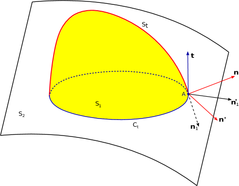
Figure 1: A drop lies on solid surface $\mathcal{S}=S_{1}\cup S_{2}$ ; $S_{t}$ is a free surface; $\mathbf{n}_{1}$ and $\mathbf{n}$ are the external unit normal vectors to $S_{1}$ and $S_{t}$, respectively. Contact line $C_{t}$ separates $S_{1}$ and $S_{2}$, $\mathbf{t}$ is the unit tangent vector to $C_{t}$ on $\mathcal{S}$. Vectors $\mathbf{n}^{\prime}_{1}=\mathbf{n}_{1}\times\mathbf{t}$ and $\mathbf{n}^{\prime}=\mathbf{t}\times\boldsymbol{n}$ are the binormals to $C_{t}$ relatively to $\mathcal{S}$ and $S_{t}$ at point $A$ of $C_{t}$, respectively.

One can formulate the virtual work principle in the form Germain_1973 ; Gouin_2007 :

$$\delta{\cal A}_{e}+\delta{\cal A}_{i}-\delta{\cal E}=0,$$

where $\delta{\cal A}_{e}$ is the virtual work of external forces, $\delta{\cal A}_{i}$ is the virtual work of inertial forces, and $\delta{\cal E}$ is the variation of the total energy. The energy ${\cal E}$ is taken in the form :

$${\cal E}=\iiint_{D_{t}}\rho\,\varepsilon\,dv+\iint_{S_{t}}\sigma\,ds+\iint_{S_{1}}\sigma_{1}\,ds,$$

where specific internal energy $\varepsilon$ is a function of density $\rho$. As we mentioned before, one can also include in this dependence several scalar quantities which are transported by the flow (specific entropy, mass fractions of surfactants, etc.). From Lemma 2, Eq. (11) and the mass conservation law :

$$\rho\,{\rm det}\,\mathbf{F}=\rho_{0}(\mathbf{X}),$$

we obtain the variation of the specific energy and density at fixed Lagrangian coordinates in the form :

$$\delta\varepsilon=\frac{p}{\rho^{2}}\,\delta\rho\quad{\rm with}\quad\delta\rho=-\rho\,{\rm div}{\boldsymbol{\zeta}},$$

where $p$ is the thermodynamical pressure. Consequently, the variation of the first term is Berdichevsky ; Gavrilyuk ; Serrin :

$$\delta\iiint_{D_{t}}\rho\,\varepsilon\,dv = \delta\iiint_{D_{0}}\rho_{0}\,\varepsilon\,dv_{0}=\iiint_{D_{0}}\rho_{0}\,\delta\varepsilon\,dv_{0}$$

$$= \iiint_{D_{t}}\rho\,\delta\varepsilon\,dv=-\iiint_{D_{t}}p\ {\rm div}\,{\boldsymbol{\zeta}}\,dv.$$

The variation of the surface energy is given in Lemma 3. The third term is the surface energy of $S_{1}$ with energy $\sigma_{1}$ per unit surface. The virtual work of the external forces is given in the form :

$$\delta{\cal A}_{e}=\iiint_{D_{t}}\rho\,\mathbf{f}^{T}{\boldsymbol{\zeta}}dv+\iint_{S_{t}}\mathbf{T}^{T}{\boldsymbol{\zeta}}ds+\int_{C_{t}}\sigma_{2}{\mathbf{n}_{1}^{\prime T}}\boldsymbol{\zeta}ds,$$

where $\rho\,\mathbf{f}$ is the volume external force in $D_{t}$, $\mathbf{T}$ is the external stress vector at the free surface $S_{t}$, and $\sigma_{2}\,{\mathbf{n}_{1}^{\prime}}$ is the line tension vector exerted on $C_{t}$. The last term on the right-hand side comes from Lemma 3 which can be also applied for rigid surfaces. Finally,

$$\delta{\cal A}_{i}=-\iiint_{D_{t}}\rho\,\mathbf{a}^{T}{\boldsymbol{\zeta}}dv$$

is the virtual work of inertial force, where $\mathbf{a}$ is the acceleration. The virtual work of forces $\delta\mathcal{T}$ applied to the material volume $D_{t}$ is defined as :

$$\delta\mathcal{T} = \displaystyle\iiint_{D_{t}}\left(-\rho\,\mathbf{a}^{T}+\rho\,\mathbf{f}^{T}-\mathbf{}\boldsymbol{\nabla}^{T}p\right)\boldsymbol{\zeta\ }dv+\iint_{S_{1}}\left(p+H_{1}\sigma_{1}\right)\mathbf{n}_{1}^{T}\boldsymbol{\zeta}\,ds$$

$$+ \iint_{S_{t}}\bigg{[}\,-{\rm div_{tg}}\left(\frac{\partial\sigma}{\partial\mathbf{R}}\mathbf{R}\right)+{\rm div_{tg}}\left(\mathbf{P}\frac{\partial\sigma}{\partial\mathbf{R}}\right)\mathbf{R}$$

$$- \,{\rm div_{tg}}\left(\mathbf{P}\,{\rm div_{tg}^{\it T}}\left(\mathbf{P}\frac{\partial\sigma}{\partial\mathbf{R}}\right)\right)\mathbf{n}^{T}+\left(p+H\sigma\right)\mathbf{n}^{T}+\boldsymbol{\nabla}_{\rm tg}^{T}\sigma+\mathbf{T}^{T}\bigg{]}\boldsymbol{\zeta}\,ds$$

$$- \int_{C_{t}}\left\{\left[\left(\sigma_{1}-\sigma_{2}\right)\mathbf{n}_{1}^{\prime T}+\sigma\,\mathbf{n}^{\prime T}-\mathbf{n}^{\prime T}{\rm div}_{\rm tg}^{T}\left(\mathbf{P}\frac{\partial\sigma}{\partial\mathbf{R}}\right)\mathbf{n}^{T}-\mathbf{n}^{\prime T}\frac{\partial\sigma}{\partial\mathbf{R}}{\mathbf{R}}\right]\boldsymbol{\zeta}\right.$$

$$\qquad\ \ +\left.\mathbf{n}^{\prime T}\frac{\partial\sigma}{\partial\mathbf{R}}\,\mathbf{P}\left(\frac{\partial\boldsymbol{\zeta}}{\partial\mathbf{x}}\right)^{T}\mathbf{n}\right\}dl.$$

As usually, $H_{1}$ and $H$ are the sum of principle curvatures of surfaces $S_{1}$ and $S_{t}$, respectively. Terms on $D_{t}$, $S_{1}$, $S_{t}$ are in separable form with respect to the field $\boldsymbol{\zeta}$. Expression (6) implies the equation of motion in $D_{t}$ and boundary conditions on surfaces $S_{1}$, $S_{t}$ Schwartz . Virtual displacement $\boldsymbol{\zeta}$ must be compatible with conditions of the problem; for example, $S_{1}$ is an external surface to domain $D_{t}$ and consequently $\boldsymbol{\zeta}$ must be tangent to $S_{1}$. This notion is developed in Berdichevsky . They are presented below.

6.1 Equation of motion

We consider virtual displacements $\boldsymbol{\zeta}$ which vanish on the boundary of $D_{t}$. The fundamental lemma of virtual displacements yields :

$$\rho\,\mathbf{a}+{\nabla}p=\rho\,\mathbf{f},\$$ (21)

which is the classical Newton law in continuum mechanics.

6.2 Condition on surface $S_{1}$

Due to the fact that the surface $S_{1}$ is - a priori - given, the virtual displacements must be compatible with the geometry of $S_{1}$. This means that the non-penetration condition (slip condition) is verified :

$$\mathbf{n}_{1}^{T}\boldsymbol{\zeta}=0.$$ (22)

Constraint (22) is equivalent to the introduction of a Lagrange multiplier $\mathcal{P}_{1}$ into (6) where $\boldsymbol{\zeta}$ is now a virtual displacement without constraint. The corresponding term on $S_{1}$ will be modified into

$$\iint_{S_{1}}\left(p+H_{1}\sigma_{1}-\mathcal{P}_{1}\right)\mathbf{n}_{1}^{T}\boldsymbol{\zeta}\,ds.$$

Since the variation of $\boldsymbol{\zeta}$ on $S_{1}$ is independent, Eq. (6) implies :

$$\mathcal{P}_{1}=p+H_{1}\sigma_{1}.$$ (23)

This is the classical Laplace condition allowing us to obtain the normal stress component $\mathcal{P}_{1}\mathbf{n}_{1}$ exerted by surface $S_{1}$.

6.3 Extended shape equation

Taking account of Eqs. (21) and (23), for all displacement $\boldsymbol{\zeta}$ on moving membrane $S_{t}$, one has from Eq. (6) :

$$\iint_{S_{t}}\bigg{[}\,-{\rm div_{tg}}\left(\frac{\partial\sigma}{\partial\mathbf{R}}\,\mathbf{R}\right)+{\rm div_{tg}}\left(\mathbf{P}\,\frac{\partial\sigma}{\partial\mathbf{R}}\right)\mathbf{R}$$

$$- \,{\rm div_{tg}}\left(\mathbf{P}\,{\rm div_{tg}^{\it T}}\left(\mathbf{P}\frac{\partial\sigma}{\partial\mathbf{R}}\right)\right)\mathbf{n}^{T}+\left(p+H\sigma\right)\mathbf{n}^{T}+\boldsymbol{\nabla}_{\rm tg}^{T}\sigma+\mathbf{T}^{T}\bigg{]}\boldsymbol{\zeta}\,ds=0.$$

It implies :

$$\left\{p+H\sigma-{\rm div_{tg}}\left[\mathbf{P}\,{\rm div_{tg}^{\it T}}\left(\mathbf{P}\frac{\partial\sigma}{\partial\mathbf{R}}\right)\right]\right\}\mathbf{n}$$

$$+{\nabla}_{\rm tg}\sigma-\,{\rm div_{tg}^{\it T}}\left(\frac{\partial\sigma}{\partial\mathbf{R}}\mathbf{R}\right)+\mathbf{R}\,{\rm div_{tg}^{\it T}}\left(\mathbf{P}\frac{\partial\sigma}{\partial\mathbf{R}}\right)+\mathbf{T}=0.$$ (24)

Equation (24) is the most general form of the dynamical boundary condition on $S_{t}$. Due to the fact that surface energy $\sigma$ must be an isotropic function of curvature tensor $\mathbf{R}$, i.e. a function of two invariants $H$ and $K$, we obtain (for proof, see Appendix) that the following vector

$${\nabla}_{\rm tg}\sigma-{\rm div_{tg}^{\it T}}\left(\frac{\partial\sigma}{\partial\mathbf{R}}\mathbf{R}\right)+\mathbf{R}\,{\rm div_{tg}^{\it T}}\left(\mathbf{P}\frac{\partial\sigma}{\partial\mathbf{R}}\right)$$

is normal to $S_{t}$ and consequently $\mathbf{T}$ writes in the form :

$$\mathbf{T}=-\mathcal{P}\,\mathbf{n}.$$

Here scalar $\mathcal{P}$ has the dimension of pressure.
One obtains from Eq. (44) (see Appendix) :

$$\displaystyle H\sigma-\Delta_{\mathrm{tg}}a - b\,\Delta_{\mathrm{tg}}H-\nabla_{\mathrm{tg}}^{T}b\,\nabla_{\mathrm{tg}}H-\mathrm{div_{tg}}\left(\mathbf{R}\,\nabla_{\mathrm{tg}}b\right)$$ (25)

$$+ \left(2K-H^{2}\right)\frac{\partial\sigma}{\partial H}-HK\frac{\partial\sigma}{\partial K}=\mathcal{P}-p.$$

Relation (25) is the normal component of Eq. (24).
It is important to underline that equation (24) is only expressed in the normal direction to $S_{t}$. This is not the case when surface energy $\sigma$ also depends on physico-chemical characteristics of $S_{t}$, as temperature or surfactants. In this last case, Marangoni effects can appear producing additive tangential terms to $S_{t}$.
Using Lemma 1 (second equation) and expressions of scalars $a$ and $b$ given by Eq. (16), we get the extended shape equation:

$$H \left(\sigma-K\frac{\partial\sigma}{\partial K}\right)+\left(2K-H^{2}\right)\frac{\partial\sigma}{\partial H}-\Delta_{\rm tg}\frac{\partial\sigma}{\partial H}-H\,\Delta_{\rm tg}\frac{\partial\sigma}{\partial K}$$ (26)

$$- \nabla_{\mathrm{tg}}^{T}H\,\nabla_{\mathrm{tg}}\frac{\partial\sigma}{\partial K}\,+\mathrm{div_{tg}}\left(\mathbf{R}\,\nabla_{\mathrm{tg}}\frac{\partial\sigma}{\partial K}\right)=\mathcal{P}-p.$$

Equation (26) was also derived in virga under the hypothesis (10) and the assumption of inextensibility of the membrane. Our derivation does not use these hypotheses. For example, the inextensibility property is not natural even in the case of incompressible fluids (at fixed volume, the surface of a 3D body may vary).

6.4 Helfrich’s shape equation

The Helfrich energy is given by Eq. (1). The shape equation (26) immediately writes in the form :

$$\sigma_{0}\,H+\frac{\kappa}{2}\left(H-H_{0}\right)\left[4K-H\left(H+H_{0}\right)\right]-\kappa\,\Delta_{\rm tg}\,H=\mathcal{P}-p\,,$$ (27)

which is the classical form obtained by Helfrich .

7 Extended Young-Dupré condition on contact line $C_{t}$

Let us denote by $\theta=\left\langle\mathbf{n}^{\prime},\mathbf{n}^{\prime}_{1}\right\rangle=\pi+\left\langle\mathbf{n},\mathbf{n}_{1}\right\rangle[{\rm mod}\,2\pi]$ the Young angle between $S_{1}$ and $S_{t}$ (see Fig. 2).

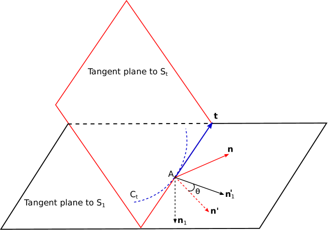
Figure 2: Tangent planes to membrane $S_{t}$ and solid surface $S_{1}$ : $\mathbf{n}_{1}$ and $\mathbf{n}$ are the unit normal vectors to $\mathcal{S}$ and $S_{t}$, external to the domain of the vesicle; contact line $C_{t}$ is shared between $\mathcal{S}$ and $S_{t}$ and $\mathbf{t}$ is the unit tangent vector to $C_{t}$ relatively to $\mathbf{n}$; $\mathbf{n}^{\prime}_{1}=\mathbf{n}_{1}\times\mathbf{t}$ and $\mathbf{n}^{\prime}=\mathbf{t}\times\boldsymbol{n}$ are binormals to $C_{t}$ relatively to $\mathcal{S}$ and $S_{t}$ at point $A$, respectively. Angle $\theta=\left\langle\mathbf{n}^{\prime},\mathbf{n}^{\prime}_{1}\right\rangle$. The normal plane to $C_{t}$ at A contains vectors $\mathbf{n},\mathbf{n}^{\prime},\mathbf{n}_{1},\mathbf{n}_{1}^{\prime}$.

Due to the fact that $C_{t}$ belongs to $S_{1}$, the virtual displacement on $C_{t}$ is in the form :

$$\boldsymbol{\zeta}=\alpha\mathbf{t}+\beta\mathbf{n}^{\prime}_{1},$$ (28)

where $\alpha$ and $\beta$ are two scalar fields defined on $S_{1}$. Let us remark that condition (28) expresses the non-penetration condition (22) on $S_{1}$. Moreover, since $\mathbf{n}$, $\mathbf{n}_{1}$, $\mathbf{n}_{1}^{\prime}$ belong to the normal plane to $C_{t}$ at $A$ (see Fig. 2), one has :

$$\boldsymbol{n}=\boldsymbol{n}_{1}^{\prime}\sin\;\theta-\boldsymbol{n}_{1}\cos\;\theta.$$ (29)

But relation $\boldsymbol{\zeta}^{T}\boldsymbol{n}_{1}=0$ implies

$$\mathbf{P}\left(\frac{\partial\boldsymbol{\zeta}}{\partial\mathbf{x}}\right)^{T}\mathbf{n}_{1}+\mathbf{P}\left(\frac{\partial\mathbf{n}_{1}}{\partial\mathbf{x}}\right)^{T}\boldsymbol{\zeta}=0.$$

Replacing (29) into (6) one has :

$$\displaystyle\delta\mathcal{T}=-\int_{C_{t}}\left\{\left[\left(\sigma_{1}-\sigma_{2}\right)\mathbf{n}_{1}^{\prime T}+\sigma\,\mathbf{n}^{\prime T}-\mathbf{n}^{\prime T}{\rm div}_{\rm tg}^{T}\left(\mathbf{P}\frac{\partial\sigma}{\partial\mathbf{R}}\right)\mathbf{n}^{T}-\mathbf{n}^{\prime T}\frac{\partial\sigma}{\partial\mathbf{R}}{\mathbf{R}}\right]\boldsymbol{\zeta}\right.$$

$$\qquad\ \ +\left.\mathbf{n}^{\prime T}\frac{\partial\sigma}{\partial\mathbf{R}}\,\mathbf{P}\left(\frac{\partial\boldsymbol{\zeta}}{\partial\mathbf{x}}\right)^{T}\mathbf{n}\right\}dl=$$

$$-\int_{C_{t}}\left\{\left[\left(\sigma_{1}-\sigma_{2}\right)\mathbf{n}_{1}^{\prime T}+\sigma\,\mathbf{n}^{\prime T}-\mathbf{n}^{\prime T}{\rm div}_{\rm tg}^{T}\left(\mathbf{P}\frac{\partial\sigma}{\partial\mathbf{R}}\right)\mathbf{n}^{T}-\mathbf{n}^{\prime T}\frac{\partial\sigma}{\partial\mathbf{R}}{\mathbf{R}}+{\color[rgb]{0,0,0}\cos}\,\theta\,\mathbf{n}^{\prime T}\frac{\partial\sigma}{\partial\mathbf{R}}{\mathbf{P}}\,\left(\frac{\partial\mathbf{n}_{1}}{\partial\mathbf{x}}\right)^{T}\right]\boldsymbol{\zeta}\right.$$

$$\qquad\ \ +\ {\sin}\,\theta\,\left.\mathbf{n}^{\prime T}\frac{\partial\sigma}{\partial\mathbf{R}}\,\mathbf{P}\left(\frac{\partial\boldsymbol{\zeta}}{\partial\mathbf{x}}\right)^{T}\mathbf{n}_{1}^{\prime}\right\}dl=0.$$ (30)

We choose now the virtual displacement in the form $\boldsymbol{\zeta}=\beta\;{\mathbf{n}}_{1}^{\prime}$. One has :

$$\frac{\partial\boldsymbol{\zeta}}{\partial\mathbf{x}}={\mathbf{n}}_{1}^{\prime}\;(\nabla\beta)^{T}+\beta\;\frac{\partial{\mathbf{n}}_{1}^{\prime}}{\partial\mathbf{x}},\quad\left(\frac{\partial\boldsymbol{\zeta}}{\partial\mathbf{x}}\right)^{T}=\nabla\beta\;{\mathbf{n}}_{1}^{\prime T}+\beta\;\left(\frac{\partial{\mathbf{n}}_{1}^{\prime}}{\partial\mathbf{x}}\right)^{T}.$$

Since $\displaystyle{\left(\frac{\partial{\mathbf{n}}_{1}^{\prime}}{\partial\mathbf{x}}\right)^{T}{\mathbf{n}}_{1}^{\prime}}=0$, it implies :

$$\left(\frac{\partial\boldsymbol{\zeta}}{\partial\mathbf{x}}\right)^{T}{\mathbf{n}}_{1}^{\prime}=\nabla\beta.$$

The integral (30) becomes :

$$\displaystyle\displaystyle\int_{C_{t}}\left\{\left[\left(\sigma_{1}-\sigma_{2}\right)\mathbf{n}_{1}^{\prime T}+\sigma\,\mathbf{n}^{\prime T}-\mathbf{n}^{\prime T}{\rm div}_{\rm tg}^{T}\left(\mathbf{P}\frac{\partial\sigma}{\partial\mathbf{R}}\right)\mathbf{n}^{T}-\mathbf{n}^{\prime T}\frac{\partial\sigma}{\partial\mathbf{R}}{\mathbf{R}}+{\color[rgb]{0,0,0}\cos}\,\theta\,\mathbf{n}^{\prime T}\frac{\partial\sigma}{\partial\mathbf{R}}{\mathbf{P}}\,\left(\frac{\partial\mathbf{n}_{1}}{\partial\mathbf{x}}\right)^{T}\right]\mathbf{n}_{1}^{\prime}\;\beta\right.$$

$$\qquad\ \ +\ {\sin}\,\theta\,\left.\mathbf{n}^{\prime T}\frac{\partial\sigma}{\partial\mathbf{R}}\,\mathbf{P}\;\nabla\beta\right\}dl=0.$$ (31)

Since $\beta$ and the components of $\nabla\beta$ can be choosen as independent, relation (31) implies two boundary conditions. The first condition on line $C_{t}$ is :

$${\rm sin}\,\theta\,\mathbf{n}^{\prime T}\frac{\partial\sigma}{\partial\mathbf{R}}\,\mathbf{P}=0.$$ (32)

The second condition is :

$$\left[\left(\sigma_{1}-\sigma_{2}\right)\mathbf{n}_{1}^{\prime T}+\sigma\,\mathbf{n}^{\prime T}-\mathbf{n}^{\prime T}{\rm div}_{\rm tg}^{T}\left(\mathbf{P}\frac{\partial\sigma}{\partial\mathbf{R}}\right)\mathbf{n}^{T}-\mathbf{n}^{\prime T}\frac{\partial\sigma}{\partial\mathbf{R}}{\mathbf{R}}+{\color[rgb]{0,0,0}\cos}\,\theta\,\mathbf{n}^{\prime T}\frac{\partial\sigma}{\partial\mathbf{R}}{\mathbf{P}}\,\left(\frac{\partial\mathbf{n}_{1}}{\partial\mathbf{x}}\right)^{T}\right]\mathbf{n}_{1}^{\prime}=0.$$ (33)

The case ${\rm sin}\,\theta=0$ all along $C_{t}$ is degenerate. If $\theta=0$, this corresponds to a hydrophobic surface (the contact line is absent). If $\theta=\pi$, this corresponds to a complete wetting. In the last case ${\mathbf{n}}_{1}^{\prime}=-{\mathbf{n}}^{\prime}$, ${\mathbf{n}}_{1}={\mathbf{n}}$, and the condition (33) becomes trivial : $\sigma_{1}-\sigma_{2}-\sigma=0$.

The general case corresponds to the partial wetting ($\sin\;\theta\neq 0$). Due to Eq. (18),

$$\mathbf{n}^{\prime T}\frac{\partial\sigma}{\partial\mathbf{R}}\,\mathbf{P}\equiv\mathbf{n}^{\prime T}(a\;\mathbf{I}+b\,\mathbf{R})\mathbf{P}\equiv a\,\mathbf{n}^{\prime T}+b\,\mathbf{n}^{\prime T}\mathbf{R}\equiv\mathbf{n}^{\prime T}\frac{\partial\sigma}{\partial\mathbf{R}}.$$

Hence, Eq. (32) yields

$$\mathbf{n}^{\prime T}\frac{\partial\sigma}{\partial\mathbf{R}}=0.$$ (34)

Equation (34) implies (see Lemma 4) :

$$\mathbf{n}^{\prime T}\left[\left(\frac{\partial\sigma}{\partial H}+H\frac{\partial\sigma}{\partial K}\right)\mathbf{I}-\frac{\partial\sigma}{\partial K}\mathbf{R}\right]=0.$$

Consequently, $\mathbf{n}^{\prime}$ is an eigenvector of $\mathbf{R}$. We denote $c_{n^{\prime}}$ the associated eigenvalue $c_{2}$. Then

$$\frac{\partial\sigma}{\partial H}+H\frac{\partial\sigma}{\partial K}=c_{n^{\prime}}\frac{\partial\sigma}{\partial K}.$$ (35)

Due to the fact that $\mathbf{t}$ is also eigenvector of $\mathbf{R}$ with eigenvalue $c_{t}=c_{1}$ ($\mathbf{t}$ and $\mathbf{n}^{\prime}$ form the eigenbasis of $\mathbf{R}$ along $C_{t}$), we get $H=c_{t}+c_{n^{\prime}}$ and the equivalent to the boundary condition (35) in the form :

$$\frac{\partial\sigma}{\partial H}+c_{t}\frac{\partial\sigma}{\partial K}=0.$$ (36)

From Lemma 4, Eq. (16), we immediately deduce :

$${\rm div_{tg}}\left(\mathbf{P}\frac{\partial\sigma}{\partial\mathbf{R}}\right)=\nabla_{\rm tg}^{T}a+\left(a\,H+b\,H^{2}-2\,b\,K\right)\mathbf{n}^{T}+\nabla_{\rm tg}^{T}b\ \mathbf{R}+b\,\nabla_{\rm tg}^{T}H.$$ (37)

Due to the fact that $\mathbf{n}^{\prime T}\mathbf{n}=0$, we obtain :

$$\mathbf{n}^{\prime T}\,{\rm div}_{\rm tg}^{T}\left(\mathbf{P}\frac{\partial\sigma}{\partial\mathbf{R}}\right)=\mathbf{n}^{\prime T}\left[\nabla_{\rm tg}a+\mathbf{R}\,\nabla_{\rm tg}b+b\,\nabla_{\rm tg}H\right]=\mathbf{n}^{\prime T}\left[\nabla a+\mathbf{R}\,\nabla b+b\,\nabla H\right]$$

Consequently, one obtains the second condition on $C_{t}$ in the form :

$$\sigma_{1}-\sigma_{2}+\sigma\,{\rm cos}\,\theta{\color[rgb]{0,0,0}-}{\rm sin}\,\theta\,\mathbf{n}^{\prime T}\left(\nabla a+b\,\nabla H+\mathbf{R}\,\nabla b\right)=0.$$ (38)

This is the extended Young-Dupré condition along contact line $C_{t}$ between membrane $S_{t}$ and solid surface $\mathcal{S}$ ().
In the case of Helfrich’s energy given by relation (1), we obtain the extended Young-Dupré condition (38) in the form :

$$\sigma_{1}-\sigma_{2}+\sigma\,{\rm cos}\,\theta{\color[rgb]{0,0,0}-}\kappa\,{\rm sin}\,\theta\,\mathbf{n}^{\prime T}\nabla H=0.$$ (39)

This last condition was previously obtained in Gouin_2014_vesicle .

8 Surfaces of revolution

8.1 Shape equation for the surfaces of revolution

Along a revolution surface, the invariants of the curvature tensor depend only on $s$ which is the curvilinear abscissa of meridian curve denoted by $\Gamma$ Aleksandrov :

$$H=H(s),\quad K=K(s).$$

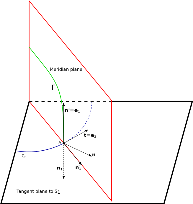
Figure 3: The case of a revolution domain. The line $C_{t}$ (contact edge between $S_{t}$ and $S_{1}$) is a circle with an axis which is the revolution axis collinear to ${\mathbf{n}}_{1}$. The meridian curve is denoted $\Gamma$; normal vector ${\mathbf{n}}$ and binormal vector ${\mathbf{n}}^{\prime}$ are in the meridian plane of revolution surface $S_{t}$. We have $\mathbf{n}^{\prime}=\mathbf{e}_{1}$ and $\mathbf{t}=\mathbf{e}_{2}$, corresponding to the eigenvectors of the curvature tensor $\mathbf{R}$ at $A$.

One of the eigenvectors, denoted ${\mathbf{e}}_{1}$, of the curvature tensor $\mathbf{R}$ is tangent to meridian curve $\Gamma$ (see Fig. 3). Let us remark that for any function $f(s)$, one has :

$$\nabla_{\mathrm{tg}}\,f=\frac{df}{ds}\,\mathbf{e}_{1},\quad\Delta_{\mathrm{tg}}\,f=\frac{d^{2}f}{ds^{2}}.$$

Indeed, the first equation is the definition of the tangential gradient. The second equality is obtained as follows :

$${\rm div}_{\mathrm{tg}}\left(\frac{df}{ds}{\mathbf{e}}_{1}\right)={\rm tr}\left({\mathbf{P}}\frac{\partial}{\partial{\mathbf{x}}}\left(\frac{df}{ds}{\mathbf{e}}_{1}\right)\right)={\rm tr}\left({\mathbf{P}}\frac{d}{ds}\left(\frac{df}{ds}{\mathbf{e}}_{1}\right)\otimes{\mathbf{e}}_{1}\right)$$

$$={\rm tr}\left(\frac{d^{2}f}{ds^{2}}{\mathbf{P}}{\mathbf{e}}_{1}\otimes{\mathbf{e}}_{1}+c_{1}(s)\frac{df}{ds}{\mathbf{n}}\otimes{\mathbf{e}}_{1}\right)=\frac{d^{2}f}{ds^{2}}.$$

The Frénet formula was used here :

$$\frac{d{\mathbf{e}}_{1}}{ds}=c_{1}{\mathbf{n}}.$$

Also,

$${\rm div}_{\mathrm{tg}}\left(\mathbf{R}\nabla_{\mathrm{tg}}\,f\right)={\rm div}_{\mathrm{tg}}\left(\frac{df}{ds}\mathbf{R}{\mathbf{e}}_{1}\right)={\rm div}_{\mathrm{tg}}\left(\frac{df}{ds}c_{1}{\mathbf{e}}_{1}\right)=\frac{d}{ds}\left(c_{1}\displaystyle{\frac{df}{ds}}\right).$$

For surfaces of revolution the shape equation (26) becomes :

$$H \left(\sigma-K\frac{\partial\sigma}{\partial K}\right)+\left(2K-H^{2}\right)\frac{\partial\sigma}{\partial H}-\frac{d^{2}}{ds^{2}}\left(\frac{\partial\sigma}{\partial H}\right)-H\,\frac{d^{2}}{ds^{2}}\left(\frac{\partial\sigma}{\partial K}\right)$$

$$- \frac{dH}{ds}\frac{d}{ds}\left(\frac{\partial\sigma}{\partial K}\right)+\frac{d}{ds}\left(c_{1}\frac{d}{ds}\left(\frac{\partial\sigma}{\partial K}\right)\right)=\mathcal{P}-p.$$

8.2 Extended Young–Dupré condition for surfaces of revolution

One has along $C_{t}$, ${\mathbf{t}}={\mathbf{e}}_{2}$, ${\mathbf{n}}^{\prime}={\mathbf{e}}_{1}$. It implies ${\mathbf{n}}^{\prime T}\mathbf{R}\,{\mathbf{t}}=0$. Also, one has :

$$\mathbf{n}^{\prime T}\left(\nabla a+b\,\nabla H+\mathbf{R}\,\nabla b\right)=\frac{da}{ds}+b\,\frac{dH}{ds}+c_{1}\,\frac{db}{ds}.$$

The Young – Dupré condition (38) becomes :

$$\sigma_{1}-\sigma_{2}\,{\rm cos}\,\theta{\color[rgb]{0,0,0}-}{\rm sin}\,\theta\left(\frac{da}{ds}+b\,\frac{dH}{ds}+c_{t}\,\frac{db}{ds}\right)=0.$$

Since

$$a=\frac{\partial\sigma}{\partial H}+H\frac{\partial\sigma}{\partial K},\quad b=-\frac{\partial\sigma}{\partial K},$$

one finally obtains :

$$\sigma_{1}-\sigma_{2}\,{\rm cos}\,\theta{\color[rgb]{0,0,0}-}{\rm sin}\,\theta\left[\frac{d}{ds}\left(\frac{\partial\sigma}{\partial H}\right)+c_{n^{\prime}}\frac{d}{ds}\left(\frac{\partial\sigma}{\partial K}\right)\right]=0.$$

For the Helfrich energy (1) this expression yields :

$$\sigma_{1}-\sigma_{2}\,{\rm cos}\,\theta{\color[rgb]{0,0,0}-}\kappa\frac{dH}{ds}\,{\rm sin}\,\theta=0.$$

9 Conclusion

Membranes can be considered as material surfaces endowed with a surface energy density depending on the invariants of the curvature tensor : $\sigma=\sigma(H,K)$. By using the principle of virtual working, we derived the boundary conditions on the moving membranes (“shape equation”) as well as two boundary conditions on the contact line. In limit cases, we recover classical boundary conditions. The “shape equation” and the boundary conditions are summarized below in the non-degenerate case (see (26), (36), (38)) as

• the equation for the moving surface $S_{t}$ :
  

  $\bullet\quad\displaystyle H\left(\sigma-K\frac{\partial\sigma}{\partial K}\right)+\left(2K-H^{2}\right)\frac{\partial\sigma}{\partial H}-\Delta_{\rm tg}\frac{\partial\sigma}{\partial H}-H\,\Delta_{\rm tg}\frac{\partial\sigma}{\partial K}$
  

  $\quad\ \ \displaystyle-\,\nabla_{\mathrm{tg}}^{T}H\,\nabla_{\mathrm{tg}}\frac{\partial\sigma}{\partial K}\,+\mathrm{div_{tg}}\left(\mathbf{R}\,\nabla_{\mathrm{tg}}\frac{\partial\sigma}{\partial K}\right)=\mathcal{P}-p.$
  

• the clamping condition on the moving line $C_{t}$ :
  

  $\bullet\quad\displaystyle\frac{\partial\sigma}{\partial H}+c_{t}\frac{\partial\sigma}{\partial K}=0,$
  

  Also, ($\mathbf{t}$, $\mathbf{n}$, $\mathbf{n}^{\prime}$) - which is the Darboux frame - are the eigenvectors of curvature tensor ${\mathbf{R}}$.

• dynamic generalization of the Young-Dupré condition on $C_{t}$ :
  

  $\bullet\quad\sigma_{1}-\sigma_{2}+\sigma\,{\rm cos}\,\theta{\color[rgb]{0,0,0}-}{\rm sin}\,\theta\,\mathbf{n}^{\prime T}\left(\nabla_{\rm tg}\left(\displaystyle\frac{\partial\sigma}{\partial H}\right)+\left(H{\mathbf{P}}-{\mathbf{R}}\right)\nabla_{\rm tg}\displaystyle\left(\frac{\partial\sigma}{\partial K}\right)\right)=0.$

In the case of Helfrich’s energy the generalization of Young-Dupré condition is reduced to equation (39):

$$\sigma_{1}-\sigma_{2}+\sigma\,{\rm cos}\,\theta{\color[rgb]{0,0,0}-}\kappa\;{\rm sin}\,\theta\;\mathbf{n}^{\prime T}\nabla_{\rm tg}H=0.$$

The last term, corresponding to the variation of the mean curvature of $S_{t}$ in the binormal direction at the contact line, can dominate the other terms. It could be interpreted as a line tension term usually added in the models with constant surface energy (cf. Babak ). It should also be noted that the droplet volume has no effect in the classical Young-Dupré condition. This is not the case for the generalized Young-Dupré condition since the curvatures can become very large for very small droplets (they are inversely proportional to the droplet size). The clamping condition for the Helfrich energy fixes the value of $H$ on the contact line :

$$H=H_{0}-c_{t}\frac{\bar{\kappa}}{\kappa}.$$

The new shape equation and boundary conditions can be used for solving dynamic problems. This could be, for example, the study of the “fingering” phenomenon appearing as a result of the non-linear instability of a moving contact line. This complicated problem will be studied in the future.

Acknowledgments. The authors thank the anonymous referees for their noteworthy and helpful remarks that greatly contributed to improve the final version of the paper.

10 Appendix

Since $\sigma=\sigma(H,K)$, we get :

$$\nabla_{\rm tg}\sigma=\frac{\partial\sigma}{\partial H}\nabla_{\rm tg}H+\frac{\partial\sigma}{\partial K}\nabla_{\rm tg}K.$$ (40)

From Eq. (16), we obtain :

$${\rm div_{tg}}\left(\mathbf{P}\frac{\partial\sigma}{\partial\mathbf{R}}\right)=\nabla_{\rm tg}^{T}a+\left(a\,H+b\,H^{2}-2\,b\,K\right)\mathbf{n}^{T}+\nabla_{\rm tg}^{T}b\ \mathbf{R}+b\,\nabla_{\rm tg}^{T}H.$$ (41)

Also, one has :

$${\rm div_{tg}}\left(\frac{\partial\sigma}{\partial\mathbf{R}}\,\mathbf{R}\right)={\rm div_{tg}}\left(a\,\mathbf{R}\right)+{\rm div_{tg}}\left(b\,\mathbf{R}^{2}\right).$$

Due to (9), one has :

$${\rm div_{tg}}\left(a\,\mathbf{R}\right)=(\nabla_{\rm tg}^{T}a)\ \mathbf{R}+a\,\nabla_{\rm tg}^{T}H+a\left(H^{2}-2\,K\right)\mathbf{n}^{T},$$

$${\rm div_{tg}}\left(b\,\mathbf{R}^{2}\right)={\rm div_{tg}}[b\left(H\mathbf{R}-K\mathbf{P}\right)]$$

$$=\nabla_{\rm tg}^{T}(bH)\ \mathbf{R}+b\,H\left[\nabla_{\rm tg}^{T}H+\left(H^{2}-2\,K\right)\mathbf{n}^{T}\right]-\nabla_{\rm tg}^{T}(bK)-b\,KH\mathbf{n}^{T}.$$

Consequently,

$${\rm div_{tg}}\left(\frac{\partial\sigma}{\partial\mathbf{R}}\,\mathbf{R}\right) = \left(\nabla_{\rm tg}^{T}(a+b\,H)\right)\,\mathbf{R}$$

$$+ (a+b\,H)\,\nabla_{\rm tg}^{T}H-\nabla_{\rm tg}^{T}(bK)+(aH^{2}+bH^{3}-2aK-3bHK)\mathbf{n}^{T}.$$

From relations (40), (41), (10), we deduce :

$${\nabla}_{\rm tg}\sigma-{\rm div_{tg}^{\it T}}\left(\frac{\partial\sigma}{\partial\mathbf{R}}\mathbf{R}\right)+\mathbf{R}\,{\rm div_{tg}^{\it T}}\left(\mathbf{P}\frac{\partial\sigma}{\partial\mathbf{R}}\right)=\left(2\,aK+3\,bHK-a\,H^{2}-b\,H^{3}\right)\mathbf{n}.$$

Using (41), one obtains :

$$\mathbf{P}\,{\rm div_{tg}^{\it T}}\left(\mathbf{P}\frac{\partial\sigma}{\partial\mathbf{R}}\right)=\nabla_{\rm tg}\,a+\mathbf{R}\,\nabla_{\rm tg}\,b+b\,\nabla_{\rm tg}\,H.$$

One deduces :

$${\rm div_{tg}}\left[\mathbf{P}\,{\rm div_{tg}^{\it T}}\left(\mathbf{P}\frac{\partial\sigma}{\partial\mathbf{R}}\right)\right]=\Delta_{\rm tg}a\,+{\rm div_{tg}}\left({\mathbf{R}\,\nabla_{\rm tg}b}\right)+\,b\,\Delta_{\rm tg}H+{\nabla_{\rm tg}^{T}}b\,\nabla_{\rm tg}H.$$ (43)

From relations (40), (41), (10), we deduce :

$${\nabla}_{\rm tg}\sigma-{\rm div_{tg}^{\it T}}\left(\frac{\partial\sigma}{\partial\mathbf{R}}\mathbf{R}\right)+\mathbf{R}\,{\rm div_{tg}^{\it T}}\left(\mathbf{P}\frac{\partial\sigma}{\partial\mathbf{R}}\right)=$$

$$\left(2\,a\,K+3\,b\,H\,K-a\,H^{2}-b\,H^{3}\right)\mathbf{n}$$

$$+\frac{\partial\sigma}{\partial H}\,\nabla_{\rm tg}H+\frac{\partial\sigma}{\partial K}\,\nabla_{\rm tg}K-\mathbf{R}\,\nabla_{tg}\left(a+b\,H\right)-\left(a+b\,H\right)\,\nabla_{\rm tg}H+\,\nabla_{\rm tg}(b\,K)$$

$$+\mathbf{R}\,\nabla_{tg}a+\left(a\,H+b\,H^{2}-2\,b\,K\right)\mathbf{R}\,\mathbf{n}+\mathbf{R}^{2}\,\nabla_{tg}b+b\,\mathbf{R}\,\nabla_{tg}H+\mathbf{T}={\mathbf{0}}.$$

Using relations $\mathbf{R}\,\mathbf{n}=\mathbf{0}$, Eq. (1)₃ and expressions of $a$ and $b$ given by Eq. (16), we obtain :

$$\frac{\partial\sigma}{\partial H}\,\nabla_{\rm tg}H+\frac{\partial\sigma}{\partial K}\,\nabla_{\rm tg}K-\mathbf{R}\,\nabla_{tg}\left(a+b\,H\right)-\left(a+b\,H\right)\,\nabla_{\rm tg}H+\,\nabla_{\rm tg}(b\,K)$$

$$+\mathbf{R}\,\nabla_{tg}a+\left(a\,H+b\,H^{2}-2\,b\,K\right)\mathbf{R}\,\mathbf{n}+\mathbf{R}^{2}\,\nabla_{tg}b+b\,\mathbf{R}\,\nabla_{tg}H=\mathbf{0}.$$

Consequently,

$${\nabla}_{\rm tg}\sigma-{\rm div_{tg}^{\it T}}\left(\frac{\partial\sigma}{\partial\mathbf{R}}\mathbf{R}\right)+\mathbf{R}\,{\rm div_{tg}^{\it T}}\left(\mathbf{P}\frac{\partial\sigma}{\partial\mathbf{R}}\right)=\left(2\,aK+3\,bHK-a\,H^{2}-b\,H^{3}\right)\mathbf{n}.$$

Finally, using (43), one obtains :

$$\quad\left[p+H\sigma-\Delta_{\rm tg}a-b\,\Delta_{\rm tg}H-\nabla_{\rm tg}^{T}b\ \nabla_{\rm tg}H-{\rm div_{tg}}\left(\mathbf{R}\,\nabla_{tg}b\right)\right.$$

$$\left.+\left(2\,a\,K+3\,b\,H\,K-a\,H^{2}-b\,H^{3}\right)\right]\mathbf{n}+\mathbf{T}={\mathbf{0}},$$ (44)

where all tangential terms disappear in the boundary condition on $S_{t}$.

References

(1) Alberts, B., Johnson, A., Lewis, J., Raff, M., Roberts, K., Walter, P. : Molecular biology of the cell, 4th edn. Garland Science, New York (2002).
(2) Aleksandrov, A.D., Zalgaller, V.A. : Intrinsic Geometry of Surfaces, AMS, coll. Translations of Mathematical Monographs no 15 (1967).
(3) Babak, V. G.: Stability of the lenslike liquid thickening (the drop) on a solid substrate, J. Adhesion, 80, 685–703 (2007).
(4) Berdichevsky, V. L. : Variational Principles of Continuum Mechanics: I. Fundamentals. Springer, New York (2009).
(5) Biscari, P., Canavese, S.M., Napoli, G. : Impermeability effects in three-dimensional vesicles, J. Phys. A: Math. Gen. 37, 6859–6874 (2004).
(6) Capovilla, R. Guven, J. : Stresses in lipid membranes, J. Physics A: Mathematics and General, 35, 6233-6247 (2002).
(7) Fournier, J.B. : On the stress and torque tensors in fluid membranes, Soft Matter 3, 883–888 (2007).
(8) Gavrilyuk, S., Gouin H. : A new form of governing equations of fluids arising from Hamilton’s principle, int. J. Eng. Sci. 37, 1495–1520 (1999) & arXiv:0801.2333.
(9) Gavrilyuk, S. : Multiphase Flow Modeling via Hamilton’s principle. In : Variational Models and Methods in Solid and Fluid Mechanics, CISM Courses and Lectures, v. 535 (Eds. F. dell’Isola and S. Gavrilyuk), Springer, Berlin (2011).
(10) Germain, P. : The method of the virtual power in continuum mechanics. - Part 2: microstructure, SIAM J. Appl. Math. 25, 556–575 (1973).
(11) Gouin, H. : The d’Alembert-Lagrange principle for
gradient theories and boundary conditions, in: Ruggeri, T., Sammartino, M.
(eds.), Asymptotic Methods in Nonlinear Wave Phenomena, p.p. 79-95, World Scientific, Singapore (2007) & arXiv:0801.2098.
(12) Gouin, H.: Interfaces endowed with non-constant surface energies revisited with the d’Alembert-Lagrange principle, Mathematics and Mechanics of Complex Systems, 2, 23-43 (2014) & arXiv:1311.1140.
(13) Gouin, H. : Vesicle Model with Bending Energy Revisited, Acta Appl. Math. 132, 347-358 (2014) & arXiv:1510.04824.
(14) Helfrich, W. : Elastic properties of lipid bilayers:
theory and possible experiments, Z. Naturforsch. C 28, 693–703 (1973).
(15) Lipowsky, R., Sackmann, E. (eds.) : Structure and dynamics of membranes, Handbook of Biological Physics. Vol. 1A and Vol. 1B, Elsevier, Amsterdam (1995).
(16) Napoli, G., Vergori, L. : Equilibrium of nematics vesicles, J. Phys. A: Math. Theo. 43, 445207 (2010).
(17) Ou-Yang Zhong Can, Helfrich, W. : Bending energy of vesicle membranes: General expressions for the first, second, and third variation of the shape energy and applications to spheres and cylinders, Physical Review A 39, 5280–5288 (1989).
(18) Rocard, Y. : Thermodynamique, Masson, Paris (1952).
(19) Rosso R., Virga E.G. : Adhesive borders of lipid membranes. Proceedings of the Royal Society of London A455, 41454168, (1999).
(20) Schwartz, L. : Théorie des distributions. Ch. 3,
Hermann, Paris (1966).
(21)Seifert U. : Configurations of fluid membranes and vesicles. Advances in Physics, 46, 13-137, (1997).
(22) Serrin, J. : Mathematical principles of classical fluid
mechanics, in Encyclopedia of Physics VIII/1, S. Flügge (ed.), p.p. 125-263,
Springer, Berlin (1960).
(23) Steigmann, D.J., Li, D. : Energy minimizing states of capillary systems with bulk, surface and line phases, IMA J. Appl. Math. 55, 1-17 (1995).
(24) Tu, Z. C. : Geometry of membranes, J. Geom. Symm. Phys. 24, 45-75 (2011).
(25) Willmore, T. J. : Riemannian Geometry, Clarendon Press, Oxford (1996).