Study of the effect of newly calculated phase space factor on $\beta$-decay half-lives

Abstract

We present results for $\beta$-decay half-lives based on a new recipe for calculation of phase space factors recently introduced. Our study includes $fp$-shell and heavier nuclei of experimental and astrophysical interests. The investigation of the kinematics of some $\beta$-decay half-lives is presented, and new phase space factor values are compared with those obtained with previous theoretical approximations. Accurate calculation of nuclear matrix elements is a pre-requisite for reliable computation of $\beta$-decay half-lives and is not the subject of this paper. This paper explores if improvements in calculating the $\beta$-decay half-lives can be obtained when using a given set of nuclear matrix elements and employing the new values of the phase space factors. Although the largest uncertainty in half-lives computations come from the nuclear matrix elements, introduction of the new values of the phase space factors may improve the comparison with experiment. The new half-lives are systematically larger than previous calculations and may have interesting consequences for calculation of stellar rates.

PACS numbers

23.40.Bw; 23.40.-s; 26.30.Jk

I INTRODUCTION

The precise knowledge of the $\beta$-decay rates represents an important ingredient for understanding the nuclear structure as well as the astrophysical processes like presupernova evolution of massive stars, nucleosynthesis (s-, p-, r-, rp-) processes, etc. Mol03 ; Ni14 ; Ren14 ). That is why the calculation of the $\beta$-decay half-lives in agreement with experimental results has been a challenging problem for nuclear theorists Zhi13 ; Niu13 ; Mar07 ; Hir93 ; Sta90 . Theoretically, the half-life formulas for $\beta$-decay can be expressed as a product of nuclear matrix elements (NMEs), involving the nuclear structure of the decaying parent and of the daughter nuclei, and the phase space factors (PSFs) that take into account the distortion of the electron wave function by the nuclear Coulomb field. Hence, for a precise calculation of the $\beta$-decay half-lives, an accurate computation of both these quantities is needed. The largest uncertainties come from the NME computation. In literature one can find different calculations of the NMEs for $\beta$-decays, realized for different types of transitions and final states, and with different theoretical models (e.g. based on gross theory Tak75 , QRPA approaches Sta90 ; Hir93 ; Nab99 ; Wan16 ; Ni14 ; Nik05 ; Mar07 ; Lia08 ; Niu13 ; Tan17 and shell model Mar99 ). We would not be discussing calculation of NMEs in this paper. Until recently the PSFs were considered to be calculated with enough precision and, consequently, not much attention was paid to a more rigorous calculation of them. However, recently we recomputed the PSFs for positron decay and electron capture (EC) processes for 28 nuclei of astrophysical interest, using a numerical approach Sab16 . We solved the Dirac equation (getting exact electron wave functions) with a nuclear potential derived from a realistic proton density distribution in the nucleus. We also included the screening effects. The new recipe for calculation can easily be extended to any arbitrarily heavy nuclei.

Accurate estimates of half-lives of neutron-rich nuclei have gained much interest in the recent past. This is primarily because of their key role in $r$-process nucleosynthesis. Similarly, precise value of $\beta$-decay half-lives of proton-rich nuclei is a pre-requisite for solving many astrophysical problems. In this paper, we study the effect of introducing the new PSF values, obtained with our recently introduced recipe Sab16 on the calculation of $\beta$-decay half-lives. We also extend here our previous PSF calculations (of positron decay and EC reactions) to include $\beta$-decay reactions. In order to complete the calculation of $\beta$-decay half-lives, we calculate the set of NMEs using the proton-neutron quasi-particle random phase approximation model in deformed basis and a schematic separable potential both in particle-particle and particle-hole channels. Other nuclear models and a set of improved input parameters may result in a better calculation of NMEs. However this improvement is not under the scope of current paper. We calculate both Gamow-Teller and Fermi transitions to ground and excited states, for medium and heavy nuclei of interest. We present first an investigation of the kinematics of $\beta$-decay half-lives and our PSF values are compared with those obtained with previous theoretical approximations. Later the newly computed half-lives are compared with other previous theoretical predictions and experimental data. We investigate if our new PSF values lead to any improvement in the calculated $\beta$-decay half-life values. Our present study may be extended to investigate the effect of the new PSF values on stellar decay rates, which we take as a future assignment.

This paper is organized in the following format. Section II describes the essential formalism for the calculation of PSFs and $\beta$-decay half-lives. We present our results in Section III where we also make a comparison of the current calculations with experimental data and previous calculation Gov71 . We conclude finally in Section IV.

II FORMALISM

II.1 Half Life Calculation

$\beta$-decay half-lives can be calculated as a sum over all transition probabilities to the daughter nucleus states through excitation energies lying within the Q_β value

$$T_{1/2}=(\sum_{0\leq E_{f}\leq Q_{\beta}}1/t_{f})^{-1},$$ (1)

where the partial half-lives (PHL), $t_{f}$, can be calculated using

$$t_{f}=\frac{C}{(g_{A}/g_{v})^{2}F_{A}(Z,A,E)B_{GT}(E_{f})+F_{V}(Z,A,E)B_{F}(E_{f})}.$$ (2)

In Eq. (2) value of C was taken as 6143 s Har09 , $g_{A}$, $g_{v}$ are axial-vector and vector coupling constants of the weak interaction, respectively, having $g_{A}$/$g_{v}$= -1.2694 Nak10 , while $E_{f}$ is the final state energy. $E=Q_{\beta}-E_{f}$ where $Q_{\beta}$ is the window accessible to either $\beta^{+}$-, $\beta^{-}$- or EC decay. $F_{A/V}$ are the PSFs. $B_{GT}$ and $B_{F}$ are the reduced transition probabilities for Gamow-Teller and Fermi transitions, respectively, and expressed as

$$B_{F}(E_{f})=\frac{1}{2I_{i}+1}\mid<f\parallel M_{F}\parallel i>\mid^{2},$$ (3)

$$B_{GT}(E_{f})=\frac{1}{2I_{i}+1}\mid<f\parallel M_{GT}\parallel i>\mid^{2}$$ (4)

In Eq. (3) and Eq. (4), $I_{i}$ denotes the spin of the parent state, $M_{F}$ and $M_{GT}$ are the Fermi and Gamow-Teller transition operators, respectively. Detailed calculation of the NMEs within the proton-neutron quasi-particle random phase approximation (pn-QRPA) formalism may be found in Refs. Hir93 ; Sta90 .

In this paper the NMEs calculation was performed using the pn-QRPA model. We used the Nilsson model Nil55 to calculate single particle energies and wave functions which takes into account the nuclear deformation. Pairing correlations were tackled using the BCS approach. We considered proton-neutron residual interaction in two channels, namely the particle-particle and the particle-hole interactions. Separable forms were chosen for these interactions and were characterized by interaction constants $\chi$ for particle-particle and $\kappa$ for particle-hole interactions. Here, we used the same range for $\chi$ and $\kappa$ as was discussed in Hir93 ; Sta90 . Deformation parameter values $\beta_{2}$ for all cases were taken from Ref. Ram01 . For pairing gaps we used a global approach $\Delta_{n}$ = $\Delta_{p}$ = 12/$\sqrt{A}$ [MeV]. A large model space up to 7$\hbar\omega$ was incorporated in our model to perform half-lives calculations for heavy nuclei considered in this paper.

II.2 Phase Space Factors Calculation

II.2.1 Phase space factors for $\beta^{+}/\beta^{-}$ transitions

The formalism for the PSF calculation for $\beta^{+}/\beta^{-}$ allowed transitions was discussed in detail in our previous paper Sab16 . Here, we reproduce the main features of the formalism for the sake of completion. The probability per unit time that a nucleus with atomic mass A and charge Z decays for an allowed $\beta$-branch is given by

$$\lambda_{0}=G_{\beta}^{2}/2\pi^{3}\int_{1}^{W_{0}}pW(W_{0}-W)^{2}S_{0}(Z,W)dW,$$ (5)

where $G_{\beta}$ is the weak interaction coupling constant, $p$ is the momentum of $\beta$-particle, $W$ = $\sqrt{{p^{2}+1}}$ is the total energy of $\beta$-particle and $W_{0}$ is the maximum $\beta$-particle energy. $W_{0}$ = $Q-1$ ($Q+1$) in $\beta^{+}$ ($\beta^{-}$) decay. $Q$ is the mass difference between initial and final states of neutral atoms. Eq. (5) is written in natural units ( $\hbar=m=c=1$ ), so that the unit of momentum is $mc$, the unit of energy is $mc^{2}$, and the unit of time is $\hbar$ /$mc^{2}$. The shape factors $S_{0}(Z,W)$ for allowed transitions which appear in Eq. (5) are defined as

$$S_{0}(Z,W)=\lambda_{1}(Z,W)|M_{0,1}|^{2},$$ (6)

where $M_{0,1}$ are the NMEs related to the Fermi and Gamow-Teller reduced transition probabilities as

$$|M_{0,1}|^{2}=\frac{1}{\sqrt{2I_{i}+1}}B_{F,GT},$$ (7)

and $\lambda_{1}(Z,W)$ stands for Fermi functions. For the calculation of the $\beta$-decay rates, one needs to calculate the NMEs and the PSFs that can be defined as

$$F_{\beta^{+}/\beta^{-}}=\int_{1}^{W_{0}}pW(W_{0}-W)^{2}\lambda_{1}(W)dW.$$ (8)

The above formula determines the PSFs for both the Fermi and Gamow-Teller allowed transitions, by substituting $F_{V}$ or $F_{A}$ in Eq. (2), respectively. For the allowed $\beta$-decays the Fermi functions can be expressed as

$$\lambda_{1}(Z,W)={g^{2}_{-1}+f^{2}_{1}\over 2p^{2}},$$ (9)

which is just the definition used in Ref. Gov71 (Eq. (3)), for our particular case $k=1$. We note that in the above formula a coefficient $1/(2p^{2})$ appears. Usually, this coefficient is included in the proper normalization of the wave functions, as we did. The functions $g_{-1}(Z,W)$ and $f_{1}(Z,W)$ are the large and small radial components of the positron (or electron) radial wave functions evaluated at the nuclear radius $R$. They are solutions of the coupled set of differential equations Gov71

$$\left(\frac{d}{dr}+\frac{\kappa+1}{r}\right)g_{\kappa}(W,r)=(W+V(r)+1)f_{\kappa}(W,r)$$

$$\left(\frac{d}{dr}+\frac{\kappa-1}{r}\right)f_{\kappa}(W,r)=-(W+V(r)-1)g_{\kappa}(W,r)$$ (10)

where $V(r)$ is the central potential for the positron (or the electron) and $\kappa=(l-j)(2j+1)$ is the relativistic quantum number.

Ideally, the central potential $V(r)$ from Eq. (II.2.1) should include the effects of the extended nuclear charge distribution and of the screening by orbital electrons. Unlike the recipe of Gove and Martin Gov71 , where these screening effects were treated as corrections to the wave functions, in our recipe they are included directly in the potential. This was done by deriving the potential $V(r)$ from a realistic proton density distribution in the nucleus. The charge density can be written as

$$\rho_{e}(\vec{r})=\sum_{i}(2j_{i}+1)v^{2}_{i}\left|\psi_{i}(\vec{r})\right|^{2},$$ (11)

where $\psi_{i}$ is the proton wave function of the spherical single particle state $i$ and $v_{i}$ is its occupation amplitude. The wave functions ${\psi_{i}}$, were found by solving Schrödinger equation with a Wood-Saxon potential. The $(2j_{i}+1)$ term in Eq. (11) reflects the spin degeneracy. As an example, we depict the realistic proton density for ¹²⁰Xe in cylindrical coordinates in Fig. 1(a). The profile of this proton density for the daughter nucleus ¹²⁰Xe (thick line) is compared with a constant density (dot-dashed line) in Fig. 1(b).

Figure 1: (a) Realistic proton density for ¹²⁰Xe represented in cylindrical coordinates. (b) Profile of the realistic proton density for ¹²⁰Xe (thick line) compared with that given by a constant density approximation (dot-dashed line).

Figure 2: The effective screening function $\phi_{eff}=V_{\beta^{\mp}}/V$ as function of the dimensionless distance $x$ for $Z$=54. The dashed and the dot-dashed lines correspond to $\beta^{-}$ and $\beta^{+}$ decays, respectively. The full line gives the behavior of the screening function with the boundaries $\phi(0)$=1 and $\phi(\infty)$=0, as given in Ref. Esp02 .

We integrated the realistic charge distribution over the volume of nucleus, in order to find the Coulomb potential

$$V(Z,r)=\alpha\hbar c\int\frac{\rho_{e}(\vec{r^{\prime}})}{|\vec{r}-\vec{r^{\prime}}|}d\vec{r^{\prime}}.$$ (12)

Moreover, we included the screening effect by multiplying the expression of $V(r)$ with a function $\phi(r)$, which is solution of the Thomas-Fermi equation

$$\frac{d^{2}\phi}{dx^{2}}=\frac{\phi^{3/2}}{\sqrt{x}},$$ (13)

with $x=r/b$, $b\approx 0.8853a_{0}Z^{-1/3}$ and $a_{0}$ is the Bohr radius. The solution $\phi(r)$ was calculated within the Majorana method Esp02 . In the case of $\beta^{-}/\beta^{+}$, the effective potential $V_{\beta^{\mp}}$ was modified by the screening function $\phi(r)$ as

$$rV_{\beta^{\mp}}(Z,r)=(rV(Z,r)+1)\times\phi(r)-1.$$ (14)

So, asymptotically we returned the interaction between an ion of charge $\pm 1$ of the residual nucleus, and the emitted electron/proton. The Coulomb potential in atomic units is $Z/r$ and is negative/positive for $\beta^{-}/\beta^{+}$ decays. As mentioned in Ref. Esp02 , the Thomas-Fermi equation (13) is a universal equation which does not depend on $Z$ or other physical constants. The boundaries of the screening function are $\phi(0)=1$ and $\phi(\infty)$=0. Then, the effective potential is $V_{\beta^{\mp}}(r)=V(r)$ for $r$=0, and is suppressed according to the variation of the universal screening function when $r$ increases in order to reach the asymptotic behavior $V_{\beta^{\mp}}(r)=-1/r$ for $r\rightarrow\infty$. The effective screening function is displayed in Fig. 2. Such a procedure of including the screening effect was also used previously in the computation of PSFs for double-beta decays KI13 -MPS15 and a similar behavior for the effective screening function was obtained. Essentially, effective Coulomb interactions obtained in the present work manifest the same asymptotic behavior as those obtained in Refs. KI13 ; KI12 where the Thomas-Fermi equation with a fixed boundary at infinity is solved.

We solved Eq. (II.2.1) in a screened Coulomb potential, with an accurate numerical method presented in Refs. Sal91 ; Sal95 . The method allows control of truncation errors of the solutions and the only remaining uncertainties were due to unavoidable round-off errors and due to the distortion of the potential introduced by the interpolating spline. Detailed information about this method can be found in our previous article Sab16 . Further, the integration of the PSF values was performed accurately with Gauss-Legendre quadrature in 32 points.

Because we compare our results with those of Gove and Martin Gov71 we mention selected features of their method of calculation of the PSFs. They obtained the radial electron functions ($f$, $g$) as solutions of Dirac equations for a point-nucleus and with an unscreened Coulomb spherical potential. The obtained functions were approximate, expressed in terms of $\Gamma$ functions. According to their prescriptions Gov71 , the finite nuclear size and screening effects were treated as corrections to these approximate functions.

Table 1: Comparison of PSF results calculated with our recipe (TW) and Gove and Martin recipe ($GM$), for $\beta^{+}$ decay of three virtual nuclei.

Z	A	$Q_{\beta^{+}}(MeV)$	Log($F^{(GM)}_{\beta^{+}}$)Gov71	Log($F^{(TW)}_{\beta^{+}}$)
10	20	0.05	-4.643	-4.646
		0.50	-0.700	-0.702
		5.00	3.575	3.574
50	120	0.05	-6.117	-6.195
		0.50	-1.152	-1.175
		5.00	3.319	3.311
90	230	0.05	-7.088	-7.272
		0.50	-1.330	-1.388
		5.00	3.236	3.206

Table 2: Comparison of PSF results calculated with our recipe (TW) and ($GM$), for $\beta^{-}$ decay of three virtual nuclei.

Z	A	$Q_{\beta^{-}}(MeV)$	Log($F^{(GM)}_{\beta^{-}}$)Gov71	Log($F^{(TW)}_{\beta^{-}}$)
10	20	0.05	-3.755	-3.793
		0.50	-0.366	-0.369
		5.00	3.776	3.774
50	120	0.05	-2.776	-2.978
		0.50	0.389	0.307
		5.00	4.304	4.282
90	230	0.05	-1.857	-2.026
		0.50	1.269	1.106
		5.00	4.929	4.904

In order to illustrate the differences that appears between our calculation and the approximate method of $GM$ Gov71 , we compare the PSF results for three virtual cases as discussed in Ref. Gov71 . As seen from Table 1 for $\beta^{+}$, and Table 2 for $\beta^{-}$, the differences between the two sets of PSF values may not be so obvious in the decimal logarithm scale, but in half-lives calculation where the absolute PSF values are used, the differences may be relevant as we will see in the next section.

II.2.2 Phase space factors for electron capture (EC)

Electron capture is a process which competes with positron decay. It is an alternate decay mode for the $\beta^{+}$ unstable nuclei that do not have enough energy to decay by positron emission. Considering the fact that the electron capture from the M-, N- and higher shells have negligible contributions in comparison with the K- and L- ones, we can write the PSF expression of electron capture for an allowed transition as

$$F_{EC}^{K,L_{1}}={\pi\over 2}\left(q^{2}_{K}g^{2}_{K}B_{K}+q^{2}_{L_{1}}g^{2}_{L_{1}}B_{L_{1}}\right).$$ (15)

For the $q_{K/L_{1}}$ quantities we used the expression

$$q_{K/L_{1}}=W_{EC}-\epsilon_{K/L_{1}},$$ (16)

were, $W_{EC}$ is the Q value of the $\beta^{+}$ decay in $m_{e}c^{2}$ units, $\epsilon_{i}$ are the binding energies of the 1s_1/2 and 2s_1/2 electron orbitals of the parent nucleus, $g_{i}$ their radial densities on the nuclear surface. $B_{i}\approx 1$ represent the values of the exchange correction. In our method we consider these exchange corrections to be unity, for the nuclei considered, the estimated error in doing that being under 1%. The relation $W_{0}=W_{EC}-1$ holds.

The $g_{K/L_{1}}$ are the electron bound states, solutions of the Dirac equation (II.2.1), and correspond to the eigenvalues $\epsilon_{n}$ ($n$ is the radial quantum number). The quantum number $\kappa$ is related to the total angular momentum $j_{\kappa}=\mid\kappa\mid-1/2$. These wave functions are normalized such that

$$\int_{0}^{\infty}[g^{2}_{n,\kappa}(r)+f^{2}_{n,\kappa}(r)]dr=1.$$ (17)

For the $EC$ processes, the potential used to obtain the electron wave functions reads

$$rV_{EC}(Z,r)=rV(Z,r)\phi(r),$$ (18)

and the charge number $Z=Z_{0}$ corresponds to the parent nucleus. $V(Z,r)$ is negative. More details about the numerical procedure can be found in Sab16 .

III RESULTS AND DISCUSSION

Half-lives were computed using Eq. (1) and Eq. (2). The NMEs were calculated using Eq. (3) (for Fermi transitions) and Eq. (4) (for GT transitions) within the pn-QRPA formalism. For the PSF calculation we used two different recipes. One is our newly calculation recipe Sab16 and the other one is the conventional computation using the prescription of $GM$ Gov71 . We again state that the same set of NMEs were used in both types of half-life calculations. For the $GM$ bound states, the Dirac equation is solved by assuming a Hartree self consistent Coulomb field. The finite size effect is introduced within a nuclear charge distribution of a Woods-Saxon form. In the $GM$ model, the screening is implicitly taken into account. In the calculations of this work, the Coulomb field is obtained by considering a nuclear charge distribution obtained within a shell model and a screening effect is introduced by modifying the potential. Therefore, some differences in the electron binding energies and in the wave functions arise between the two recipes. The electron energies and their radial densities on the nuclear surface for $K$ and $L_{1}$ orbitals recalculated in this work with recently improved numerical codes following the recipe of Ref. Sab16 are listed in Table 3 and compared with those of Mar70 .

The differences between the results obtained for a Coulomb field obtained from a constant charge density inside a spherical nucleus and those obtained with a field constructed with a more realistic charge density corrected with a screening function can offer an estimation of the role played by the ingredients of our model. The radial distributions of the electron $(g_{k}^{2}+f_{k}^{2})r^{2}$ are displayed in Fig. 3 for these two treatments in the case the parent nucleus ³⁸Ca. The radial distributions in the case of a pure Coulomb field, plotted with thin lines, are more confined in the vicinity of the nucleus, therefore the amplitudes of the wave function are larger. These differences are translated in the values $g^{2}_{i}$ and of the electron binding energies $\epsilon_{i}$, as it can be seen in Table 4. Adding the screening effect in our calculations makes our results very close to those of $GM$.

Figure 3: The radial distributions $(g_{k}^{2}+f_{k}^{2})r^{2}$ are plotted for the $K$ and $L_{1}$ shells as function of the distance $r$ in term of atomic units $a_{0}$ for ³⁸Ca. The thick lines are obtained with the treatment used in this work. The thin curve is used for the potential without screening and with a constant proton density inside the nucleus. The full line is used for the $K$ shell while the dashed one corresponds to the $L_{1}$ orbital.

Table 5 presents a comparison between the measured and calculated half-lives for $\beta^{+}$/EC-decay of twenty medium and heavy nuclei of interest. Entries in third column are calculated using the pn-QRPA method for the NMEs, while the PSFs are calculated by the by $(GM)$ method Gov71 . The fourth column shows the calculated half-lives using our new recipe of PSFs Sab16 and labeled $(TW)$ (this work). Most of the nuclei shown in this table are the same as those presented in Table 2 of Ref. Sab16 . All half-lives are given in units of seconds. Q-values for the reaction were taken from Aud12 . It is seen from Table 5 that the newly calculated half-lives are systematically larger than those computed using the PSFs of $(GM)$ Gov71 . The last column displays the percentage deviation (PD) of the two calculated half-lives. We calculated the PD between the two computed half-lives using the formula

$$PD=\frac{T_{1/2}^{(TW)}-T_{1/2}^{(GM)}}{T_{1/2}^{(TW)}}\times 100(\%)$$ (19)

Table 5 shows that the PD increases to a maximum value of 4.05 $\%$ for the ⁵⁶Ni nucleus. The case of EC on ²⁰⁵Bi requires special mention. For this nucleus the pn-QRPA predicts couple of high excited transitions to the daughter nucleus and the available Q-value of these two transitions is lower than the binding energy of the K-shell electron. Using calculation, after the EC process of a K-shell electron, the neutrino may have a negative energy which is not physical. Accordingly we only calculate L-shell EC in this case. In the calculated $\beta^{+}$/EC-decay half-lives, the smallest difference was noted for ⁵²Fe. In Table 6 we show the state-by-state transitions for two cases: ⁵²Fe and ⁵⁶Ni. Shown are also the adopted NMEs using the pn-QRPA model, the calculated PSFs (separately for both EC and $\beta^{+}$-decay reactions), partial half-lives (PHL), Q-values and branching ratios I${}_{(\beta^{+}/EC)}$. The branching ratio ’$I$’ for each transition was calculated using the formula

$$I=\frac{T_{1/2}}{t_{f}}\times 100(\%),$$ (20)

where T_1/2 is the total $\beta$ decay half-life and t_f is the calculated partial half-life of the corresponding transition. For the nucleus ⁵⁶Ni we note calculation of much smaller PSF for EC decay to daughter energies using our recipe. The PSFs calculated from $(GM)$ recipe is on average within 3 % smaller. This in turn led to a 4 % larger calculated half-life value for ⁵⁶Ni using our recipe.

We would like to comment further on the entries in the first two columns of Table 6. These entries are model dependent. The excited states in daughter nuclei (shown in the first column) and NMEs (presented in the second column) were calculated using the pn-QRPA model. The computed excited states satisfied the selection criteria for allowed transitions within the chosen model. A different nuclear model can change the entries in the first two columns and, as stated earlier, is not the focus of current study. Q-values are presented in the third and the sixth columns of Table 6 using following relation

$$Q_{EC}=m_{p}-m_{d}-E_{f},$$ (21)

and

$$Q_{BP}=m_{p}-m_{d}-E_{f}-2m_{e}c^{2}.$$ (22)

Here $m_{p}$ and $m_{d}$ are masses of parent and daughter nuclei, respectively whereas $E_{f}$ is the calculated energy levels in the daughter nucleus (model dependent).

Table 7 shows the comparison of measured and calculated half-lives for $\beta^{-}$ decay cases. The Q-values were taken from Aud12 . The comparison between the two calculations is much better for the $\beta^{-}$ decay half-lives than those correponding to $\beta^{+}$. Table 8 shows the state-by-state calculation of PHL for ¹⁰⁰Sr (largest PD=3.82 %) and ¹⁵²Nd (PD=2.04 %). The values of $Q_{\beta^{-}}$ (calculated as in Eq. (21)), PSF, NME and branching ratios I${}_{(\beta^{-})}$ are also given in Table 8. We note an overall agreement between our calculated PSF values and those using the $(GM)$ recipe in the case of of both analyzed nuclei.

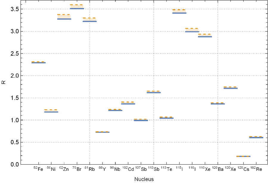
Figure 4: Ratios $R$ between experimental Aud12 and calculated half-lives undergoing $\beta^{+}$ decay for selected cases. Full lines: theoretical half-lives calculated within the $(TW)$ recipe. Dotted lines: theoretical half-lives calculated with the $(GM)$ recipe of Ref. Gov71 .

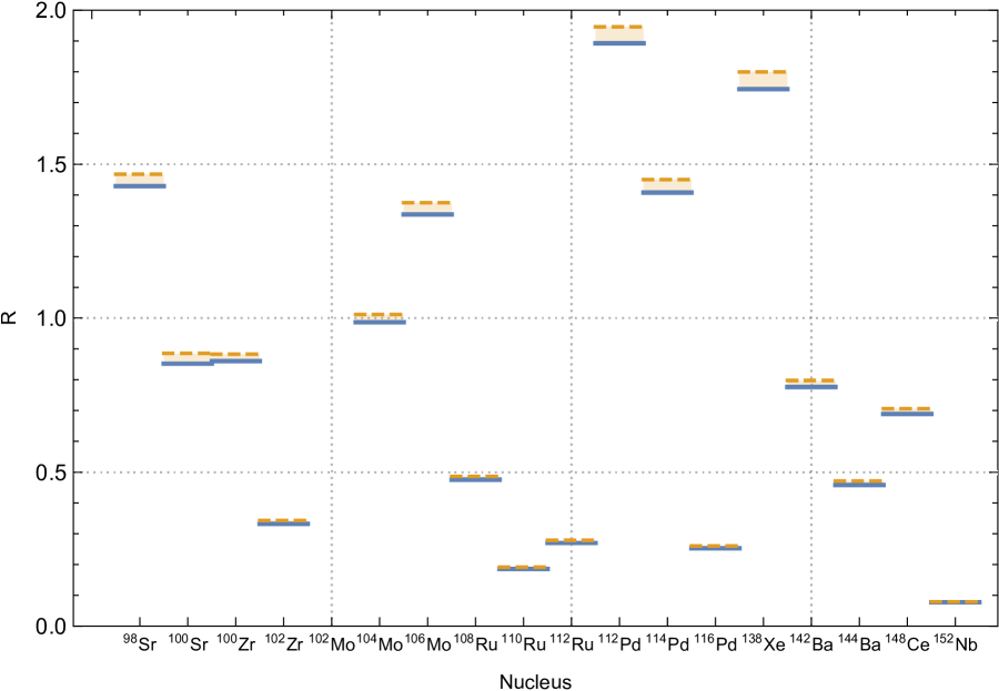
Figure 5: Same as Fig. 4 but for selected $\beta^{-}$ decay cases.

The difference between the two calculated half-lives as well as their mutual comparison with the experimental data, is done intuitively in a graphical way in Fig. 4 for few selected $\beta^{+}$ decay cases. We display the ratio between the experimental half-lives and the theoretical ones, $R=T_{1/2}^{(exp)}/T_{1/2}^{(X)}$, where $(X)$ stands for the calculation recipe, $(GM)$ or $(TW)$. With solid lines the ratios calculated with $(TW)$ recipe are represented, while with dotted lines the conventional $(GM)$ computations are displayed. We note that systematically our half-lives are larger that the $GM$, improving the agreement with the measured data for most of the cases. From Fig. 4 it can be remarked that the $(TW)$ ratios are in general closer to the value 1 than the $(GM)$ ones. This effect is highlighted in Fig. 4 by the link between the dotted line and the solid line. In Fig. 5, the ratios corresponding to $\beta^{-}$ decays are displayed in the same manner as in Fig. 4. It is noted that no appreciable improvement is brought in calculation of $\beta^{-}$ decay half-lives except for a few cases in which the experimental data are undervalued by calculations, as also evident from Table 7. Overall, we note a good agreement of the new theoretical half-lives with the experimental ones. It is again remarked that this comparison could have improved further with a more reliable set of NMEs or choice of better model parameters for the calculation of NMEs (not the subject of current paper).

The differences between the $(GM)$ and the present results can be explained by the use of a more rigorous approach in our case for the free states in the PSF computation, but also are due to the differences between our potential and the one used by $(GM)$. Regarding only the free states, in the $(GM)$ method the screening correction was introduced empirically, by modifying the solutions of the Dirac equation with a function evaluated at the nuclear surface. This function depends on the difference between the effective potential and the point like nucleus Coulomb interaction. On the other hand, in our calculation the screening is introduced by considering an effective Coulomb potential. The Dirac equation is solved numerically for this effective Coulomb potential up to large values of $r$, where the wave functions are well approximated by its asymptotic form. Later, the wave functions are normalized by comparing their value with the asymptotic forms. This normalization determines the value of each wave function on the surface of the nucleus. Further, in the $(GM)$ calculation, the nuclear finite size of the nucleus is simulated by additional corrections to the Fermi functions, while in our calculation, the effective Coulomb field is built up from the proton density of the nucleus, as also mentioned before. Regarding the bound states, the $(GM)$ method uses tabulated values of the energies and of the radial densities that are obtained by solving the Dirac equation within a more sophisticated self-consistent Coulomb potential.

IV Summary and Conclusion

The aim of present work was to investigate the effect of the incorporation of new PSF values, computed with a more precise and rigorous method, on the theoretical half-lives for $\beta^{\pm}$ and EC decays of unstable nuclei. The newly calculated $\beta$-decay half-lives were systematically larger than those given in the previous calculations. The mean percentage deviation is larger for the $\beta^{-}$ decay ($2.73\%$) as compared to the $\beta^{+}$/EC decay rates ($2.35\%$). For the adopted set of NMEs, in general the half-lives computed with newly PSFs are closer to the measured ones than the half-lives calculated with PSFs with approximate method (i.e., using approximate electron wave functions) Gov71 for free states. Although the largest uncertainty in the computation of $\beta$-decay half-lives comes from the NMEs, introduction of the newly PSF values may improve the comparison with experiment and should be taken into account for accurate predictions.

In near future we would be presenting the effect of calculation of newly computed PSF on stellar beta decay rates and comment on its astrophysical implications.

Acknowledgments

J.-U. Nabi would like to acknowledge the support of the Higher Education Commission Pakistan through project numbers 5557/KPK/NRPU/R$\&$D/HEC/2016, 9-5(Ph-1-MG-7)/PAK-TURK/R$\&$D/HEC/2017 and Pakistan Science Foundation through project number PSF-TUBITAK/KP-GIKI (02). M. Ishfaq wishes to acknowledge the support provided by Scientific and Technological Research Council of Turkey (TUBITAK), Department of Science Fellowships and Grant Programs (BIDEB) 2216 Research Fellowship Program For International Researchers (21514107-115.02-124287).

S. Stoica, M. Mirea and O. Niţescu would like to acknowledge the support of the Romanian Ministry of Research and Innovation, CNCS-UEFISCDI, through projects PN-III-P4-ID-PCE-2016-0078 and PN-5N/2018.

Table 3: The first four columns give the electron binding energies $\epsilon_{i}$ for the shells $K$ and $L_{1}$ and their radial wave function densities $g_{i}$ at the nuclear surface calculated in this work for different nuclei. The last two columns give the values of Ref. Mar70 .

Nucleus	$\epsilon_{K}$ (keV)	$\epsilon_{L_{1}}$ (keV)	$g_{K}^{2}$ ($[\hbar/mc]^{-3}$)	$g_{L_{1}}^{2}/g^{2}_{K}$	$g_{K}^{2}$ ($[\hbar/mc]^{-3}$) Mar70	$g_{L_{1}}^{2}/g^{2}_{K}$ Mar70
52Fe	6.63991	0.7451126	0.0327063	0.0898416	0.0328	0.0950
56Ni	7.95277	0.9181003	0.0411267	0.0943036	0.0423	0.0974
62Zn	9.20973	1.1092315	0.0530401	0.0953901	0.0538	0.0995
76Br	13.0121	1.6760343	0.0917936	0.1019465	0.0935	0.1035
81Rb	14.6718	1.9336296	0.1136202	0.1042520	0.1149	0.1063
88Y	16.4688	2.0221700	0.1389702	0.1272602	0.1402	0.1080
90Nb	18.3994	2.4889101	0.1686632	0.1121010	0.170	0.1098
102Cd	26.1177	3.9008765	0.3182812	0.1109908	0.319	0.1159
105Ag	24.95904	3.558919	0.2900978	0.1193451	0.293	0.1150
107Sb	29.99173	4.140248	0.4109690	0.1416423	0.413	0.1187
113Sb	29.99173	4.140248	0.4101592	0.1416413	0.413	0.1187
113Te	31.18294	4.70109	0.4488353	0.12019908	0.449	0.1196
115I	32.50419	4.937340	0.4894928	0.1210013	0.488	0.1205
116I	32.50419	4.937340	0.4893257	0.1210012	0.488	0.1205
116Xe	33.95443	5.055330	0.5289785	0.1300301	0.529	0.1215
120Ba	36.81175	4.975840	0.6244052	0.1662902	0.623	0.1234
120Xe	33.95440	5.055328	0.5280176	0.1300293	0.529	0.1215
126Cs	35.30411	5.151703	0.5764054	0.1394027	0.574	0.1224
182Re	71.29588	12.23093	2.7488862	0.1490819	2.69	0.1448
205Bi	90.39904	16.18943	5.0324494	0.1587003	4.88	0.1561

Table 4: The results $GM$ obtained in Ref. Mar70 are compared with the results $TW$ of this work and those obtained without a realistic charge density and without screening correction in the case of ³⁸Ca. The $K$ and $L_{1}$ shells are illustrated. The binding energies are denoted $\epsilon_{i}$ and the radial densities on the surface of the nucleus are denoted $g_{i}^{2}$.

Method	$\epsilon_{K}$ (keV)	$\epsilon_{L1}$ (keV)	$g_{K}^{2}$ ($[\hbar/mc]^{-3}$)	$g_{L1}^{2}/g_{K}^{2}$
Ref. Mar70	3.60740	0.37710	0.01367	0.08620
$TW$	3.762904	0.357179	0.01308474	0.0825267
No screening	5.454032	1.198887	0.01434885	0.1877057

Table 5: Comparison of measured, calculated half-lives and percentage deviation (PD) for $\beta^{+}$/EC-decay of selected nuclei. For the case of ²⁰⁵Bi we calculate only L-shell EC.

Nucleus	$T_{1/2}^{(EXP)}$ (s) Aud12	$T_{1/2}^{(GM)}$ (s) Gov71	$T_{1/2}^{(TW)}$ (s)	PD (%)
52Fe	2.98E+04	1.29E+04	1.30E+04	0.77
56Ni	5.25E+05	4.26E+05	4.44E+05	4.05
62Zn	3.31E+04	9.80E+03	1.01E+04	2.97
76Br	5.83E+04	1.62E+04	1.66E+04	2.41
81Rb	1.65E+04	5.00E+03	5.12E+03	2.34
88Y	9.21E+06	1.25E+07	1.27E+07	1.57
90Nb	5.26E+04	4.25E+04	4.32E+04	1.62
102Cd	3.30E+02	2.35E+02	2.42E+02	2.89
105Ag	3.57E+06	2.45E+04	2.52E+04	2.78
107Sb	4.00E+00	3.92E+00	4.04E+00	2.97
113Sb	4.00E+02	2.42E+02	2.47E+02	2.02
113Te	1.02E+02	9.55E+01	9.77E+01	2.25
115I	3.48E+02	9.98E+01	1.02E+02	2.16
116I	2.91E+00	9.49E-01	9.73E-01	2.47
116Xe	5.90E+01	2.01E+01	2.05E+01	1.95
120Ba	2.40E+01	1.73E+01	1.76E+01	1.70
120Xe	2.76E+03	1.58E+03	1.61E+03	1.86
126Cs	9.84E+01	5.35E+02	5.42E+02	1.29
182Re	2.30E+05	3.67E+05	3.80E+05	3.42
205Bi	1.32E+06	1.47E+06	1.52E+06	3.46

Table 6: State-by-state comparison of calculated PSF (for $\beta^{+}$/EC-decay) using recipe of Gov71 and current prescription (TW). Shown also are the daughter energy levels, nuclear matrix elements NME, $Q$ values, partial half-lives (PHL) for $\beta^{+}$/EC-decay and branching ratio I${}_{(\beta^{+}/EC)}$ of the selected nuclei.

52Fe
Ex(MeV)	NME	$Q_{EC}$ (MeV)	$F^{(GM)}_{EC}$Gov71	$F^{(TW)}_{EC}$	$Q_{\beta^{+}}$ (MeV)	$F^{(GM)}_{\beta^{+}}$Gov71	$F^{(TW)}_{\beta^{+}}$	PHL(GM)Gov71	PHL(TW)	I${}^{(GM)}_{(\beta^{+}/EC)}$ Gov71	I${}^{(TW)}_{(\beta^{+}/EC)}$
0.000	0.02768	2.3733	1.22206	1.20150	1.3512	8.41032	8.31627	1.50147E+04	1.51955E+04	85.701	85.713
0.004	0.00170	2.3693	1.21794	1.19744	1.3472	8.30402	8.21074	2.46699E+05	2.49683E+05	5.2160	5.2160
0.196	0.00325	2.1773	1.02771	1.01077	1.1552	4.29193	4.24688	2.31350E+05	2.34078E+05	5.5620	5.5640
0.291	0.00134	2.0823	0.94007	0.92425	1.0602	2.98166	2.94390	7.60563E+05	7.71098E+05	1.6920	1.6890
0.720	0.00253	1.6533	0.59198	0.58175	0.6312	0.33565	0.32942	1.70770E+06	1.73853E+06	0.7540	0.7490
0.939	0.00087	1.4343	0.44543	0.43734	0.4122	5.69E-02	5.53E-02	9.20851E+06	9.39057E+06	0.1400	0.1390
1.011	0.00350	1.3623	0.40124	0.39435	0.3402	2.53E-02	2.47E-02	2.67938E+06	2.72749E+06	0.4800	0.4780
1.362	0.00255	1.0113	0.22076	0.21663	-0.0107	-	-	7.10887E+06	7.24422E+06	0.1810	0.1800
1.467	0.00052	0.9063	0.17691	0.17374	-0.1157	-	-	4.36772E+07	4.44742E+07	0.0290	0.0290
1.685	0.00017	0.6883	1.01706E-01	9.97773E-02	-0.3371	-	-	2.35223E+08	2.39771E+08	0.0050	0.0050
1.754	0.00009	0.6193	8.22094E-02	8.06130E-02	-0.4027	-	-	5.31896E+08	5.42429E+08	0.0020	0.0020
1.821	0.00972	0.5523	6.54251E-02	6.39581E-02	-0.4697	-	-	6.29314E+06	6.43748E+06	0.2040	0.2020
2.119	0.00282	0.2543	1.35835E-02	1.32041E-02	-0.7677	-	-	1.04562E+08	1.07568E+08	0.0120	0.0120
2.143	0.00572	0.2303	1.10469E-02	1.07735E-02	-0.7917	-	-	6.33834E+07	6.49917E+07	0.0200	0.0200
56Ni
1.196	0.00038	0.9357	0.24313	0.23335	-0.0862	-	-	4.31594E+07	4.49676E+07	0.986	0.988
1.247	0.00019	0.8847	0.21729	0.20842	-0.1372	-	-	9.85234E+07	1.02717E+08	0.432	0.432
1.252	0.00034	0.8797	0.21476	0.20605	-0.1422	-	-	5.55046E+07	5.78528E+07	0.767	0.768
1.288	0.00009	0.8437	0.19721	0.18939	-0.1782	-	-	2.13703E+08	2.22525E+08	0.199	0.200
1.289	0.00009	0.8427	0.19676	0.18894	-0.1792	-	-	2.31551E+08	2.41134E+08	0.184	0.184
1.299	0.00008	0.8327	0.19227	0.18444	-0.1892	-	-	2.69031E+08	2.80450E+08	0.158	0.158
1.309	0.00001	0.8227	0.18754	0.18000	-0.1992	-	-	1.73974E+09	1.81258E+09	0.024	0.024
1.313	0.00002	0.8187	0.18593	0.17824	-0.2032	-	-	1.22606E+09	1.27894E+09	0.035	0.035
1.318	0.00001	0.8137	0.18344	0.17605	-0.2082	-	-	1.76475E+09	1.83885E+09	0.024	0.024
1.363	0.00000	0.7687	0.16374	0.15695	-0.2532	-	-	4.34936E+10	4.53747E+10	0.001	0.001
1.363	0.00000	0.7687	0.16372	0.15695	-0.2532	-	-	2.36127E+10	2.46320E+10	0.002	0.002
1.373	0.00000	0.7587	0.15927	0.15285	-0.2632	-	-	7.54380E+10	7.86020E+10	0.001	0.001
1.471	0.00000	0.6607	0.12034	0.11558	-0.3612	-	-	1.51481E+10	1.57716E+10	0.003	0.003
1.482	0.00001	0.6497	0.11645	0.11172	-0.3722	-	-	3.31503E+09	3.45531E+09	0.013	0.013
1.503	0.00001	0.6287	0.10904	0.10454	-0.3932	-	-	3.72258E+09	3.88306E+09	0.011	0.011
1.711	0.07180	0.4207	4.82788E-02	4.62700E-02	-0.6012	-	-	1.15477E+06	1.20491E+06	36.85	36.85
1.742	0.13730	0.3897	4.13076E-02	3.95910E-02	-0.6322	-	-	7.05812E+05	7.36415E+05	60.30	60.30

Table 7: Same as Table. 5 but for $\beta^{-}$-decaying nuclei.

Nucleus	$T_{1/2}^{EXP}$ (s) Aud12	$T_{1/2}^{(GM)}$ (s) Gov71	$T_{1/2}^{(TW)}$ (s)	PD (%)
98Sr	6.53E-01	4.45E-01	4.57E-01	2.63
100Sr	2.02E-01	2.28E-01	2.37E-01	3.82
100Zr	7.10E+00	8.04E+00	8.25E+00	2.55
102Zr	2.90E+00	8.45E+00	8.73E+00	3.21
102Mo	6.78E+02	1.90E+02	1.94E+02	2.06
104Mo	6.00E+00	5.93E+00	6.08E+00	2.47
106Mo	8.73E+00	6.35E+00	6.53E+00	2.76
108Ru	2.73E+02	5.61E+02	5.74E+02	2.26
110Ru	1.20E+01	6.27E+01	6.46E+01	2.94
112Ru	1.75E+00	6.27E+00	6.47E+00	3.09
112Pd	7.57E+04	3.89E+04	4.00E+04	2.75
114Pd	1.45E+02	1.00E+02	1.03E+02	2.91
116Pd	1.18E+01	4.53E+01	4.67E+01	3.00
138Xe	8.44E+02	4.69E+02	4.84E+02	3.10
140Xe	1.36E+01	1.36E+00	1.40E+00	2.86
142Ba	6.36E+02	7.97E+02	8.19E+02	2.69
144Ba	1.15E+01	2.44E+01	2.51E+01	2.79
146Ce	8.11E+02	4.74E+01	4.85E+01	2.27
148Ce	5.60E+01	7.93E+01	8.13E+01	2.46
152Nd	6.84E+02	8.64E+03	8.82E+03	2.04

Table 8: State-by-state comparison of calculated PSF (for $\beta$-decay) using recipe of Gov71 and current prescription (TW). Shown also are the daughter energy levels, nuclear matrix elements NME, $Q$ values, partial half-lives (PHL) and branching ratio I${}_{(\beta^{-})}$ for $\beta^{-}$-decay of the selected nuclei.

100Sr
Ex(MeV)	NME	$Q_{\beta^{-}}$ (MeV)	$F^{(GM)}_{\beta^{-}}$Gov71	$F^{(TW)}_{\beta^{-}}$	PHL(GM)Gov71	PHL(TW)	I${}^{(GM)}_{(\beta^{-})}$ Gov71	I${}^{(TW)}_{(\beta^{-})}$
0.13300	0.01473	7.50300	86906.3	72966.7	3.12798E+00	3.72554E+00	7.2730	6.3720
0.35700	0.00115	7.14579	69557.1	64334.6	4.99967E+01	5.40553E+01	0.4550	0.4390
0.86400	0.00510	6.63935	49775.9	47317.7	1.57827E+01	1.66026E+01	1.4410	1.4300
1.00300	0.00322	6.50023	45212.0	43184.3	2.75281E+01	2.88207E+01	0.8260	0.8240
1.06300	0.00429	6.44024	43349.3	41485.6	2.15140E+01	2.24805E+01	1.0570	1.0560
1.10400	0.00278	6.39893	42102.4	40346.8	3.42401E+01	3.57299E+01	0.6640	0.6640
1.35000	0.26502	6.15278	35247.6	33999.4	4.28548E-01	4.44280E-01	53.084	53.434
1.41900	0.01521	6.08400	33499.6	32359.0	7.85740E+00	8.13437E+00	2.8950	2.9180
1.62000	0.00002	5.88283	28778.0	27883.9	7.89102E+03	8.14407E+03	0.0030	0.0030
1.64200	0.00000	5.86112	28301.8	27429.7	2.05672E+05	2.12210E+05	0.0000	0.0000
1.66900	0.00080	5.83372	27709.5	26864.9	1.81631E+02	1.87341E+02	0.1250	0.1270
2.03600	0.03084	5.46720	20688.6	20109.3	6.27339E+00	6.45412E+00	3.6260	3.6780
2.19100	0.00096	5.31207	18180.4	17678.5	2.30158E+02	2.36693E+02	0.0990	0.1000
2.21100	0.00002	5.29152	17867.1	17374.4	1.26201E+04	1.29779E+04	0.0020	0.0020
2.21700	0.00126	5.28623	17787.1	17296.8	1.79065E+02	1.84140E+02	0.1270	0.1290
2.33500	0.01496	5.16812	16074.2	15633.6	1.66481E+01	1.71173E+01	1.3660	1.3870
2.40500	0.00704	5.09834	15125.2	14712.6	3.75885E+01	3.86428E+01	0.6050	0.6140
2.48600	0.05959	5.01712	14077.3	13695.1	4.77186E+00	4.90505E+00	4.7670	4.8400
2.55600	0.00015	4.94728	13222.8	12865.6	2.04511E+03	2.10190E+03	0.0110	0.0110
2.59700	0.00001	4.90586	12735.9	12392.7	3.58668E+04	3.68600E+04	0.0010	0.0010
2.71000	0.00051	4.79275	11477.9	11170.8	6.88307E+02	7.07229E+02	0.0330	0.0340
2.73300	0.04131	4.76967	11233.8	10933.7	8.62714E+00	8.86390E+00	2.6370	2.6780
2.92100	0.00092	4.58202	9397.47	9150.19	4.64906E+02	4.77470E+02	0.0490	0.0500
3.04900	0.00007	4.45378	8285.68	8069.38	7.37202E+03	7.56963E+03	0.0030	0.0030
3.19200	0.00721	4.31146	7176.38	6990.87	7.73167E+01	7.93683E+01	0.2940	0.2990
3.29000	0.00845	4.21307	6480.88	6314.67	7.30755E+01	7.49989E+01	0.3110	0.3170
3.29600	0.01583	4.20677	6438.24	6273.21	3.92753E+01	4.03085E+01	0.5790	0.5890
3.36400	0.00058	4.13861	5990.84	5838.16	1.15661E+03	1.18685E+03	0.0200	0.0200
3.43900	0.00029	4.06433	5531.71	5391.47	2.52582E+03	2.59152E+03	0.0090	0.0090
3.45000	0.01045	4.05281	5463.09	5324.69	7.01033E+01	7.19255E+01	0.3250	0.3300
3.47100	0.00612	4.03206	5341.13	5205.96	1.22440E+02	1.25619E+02	0.1860	0.1890
3.49600	0.00482	4.00734	5198.67	5067.29	1.59594E+02	1.63732E+02	0.1430	0.1450
3.56900	0.00134	3.93407	4794.07	4673.52	6.24537E+02	6.40647E+02	0.0360	0.0370
3.68200	0.11627	3.82086	4218.21	4112.92	8.16217E+00	8.37111E+00	2.7870	2.8360
3.88800	0.00006	3.61534	3313.42	3232.01	2.10528E+04	2.15831E+04	0.0010	0.0010
4.05100	0.01897	3.45234	2711.28	2645.88	7.78203E+01	7.97437E+01	0.2920	0.2980
4.08800	0.37148	3.41515	2586.91	2524.78	4.16561E+00	4.26810E+00	5.4610	5.5620
4.12800	0.20740	3.37510	2458.04	2399.32	7.85229E+00	8.04448E+00	2.8970	2.9510
4.16900	0.00354	3.33446	2332.50	2277.04	4.84389E+02	4.96188E+02	0.0470	0.0480
4.22200	0.00034	3.28135	2176.15	2124.70	5.47159E+03	5.60410E+03	0.0040	0.0040
4.30800	0.00556	3.19476	1939.11	1893.63	3.71131E+02	3.80044E+02	0.0610	0.0620
4.31100	0.00722	3.19210	1932.17	1886.87	2.87049E+02	2.93941E+02	0.0790	0.0810
4.40800	0.00101	3.09502	1691.86	1652.46	2.33941E+03	2.39520E+03	0.010	0.010
4.43400	0.00003	3.06860	1630.72	1592.78	8.24004E+04	8.43631E+04	0.000	0.000
4.53600	0.00007	2.96655	1410.81	1378.03	4.15176E+04	4.25053E+04	0.001	0.001
4.56000	0.00318	2.94261	1362.77	1331.13	9.23619E+02	9.45568E+02	0.025	0.025
4.62800	0.00284	2.87494	1233.96	1205.44	1.14035E+03	1.16733E+03	0.020	0.020
4.63100	0.03599	2.87213	1228.83	1200.43	9.05090E+01	9.26499E+01	0.251	0.256
4.68800	0.00938	2.81463	1127.45	1101.55	3.78490E+02	3.87390E+02	0.060	0.061
4.70300	0.01517	2.79959	1102.05	1076.78	2.39492E+02	2.45112E+02	0.095	0.097
4.78400	0.00317	2.71946	974.255	952.119	1.29597E+03	1.32610E+03	0.018	0.018
4.86000	0.33212	2.64278	863.180	843.718	1.39636E+01	1.42857E+01	1.629	1.662
4.87900	0.15890	2.62366	837.107	818.264	3.00956E+01	3.07887E+01	0.756	0.771
4.98800	0.04141	2.51538	700.916	685.342	1.37918E+02	1.41052E+02	0.165	0.168
4.99400	0.00028	2.50876	693.199	677.809	2.02785E+04	2.07390E+04	0.001	0.001
5.02400	0.00000	2.47918	659.521	644.946	2.18678E+06	2.23620E+06	0.000	0.000
5.02400	0.00000	2.47907	659.398	644.827	3.04674E+06	3.11559E+06	0.000	0.000
5.07300	0.00072	2.42998	606.361	593.032	9.17207E+03	9.37823E+03	0.002	0.003
5.07800	0.06105	2.41548	601.620	588.399	1.08997E+02	1.11446E+02	0.209	0.213
5.08800	0.00814	2.41543	591.359	578.371	8.31303E+02	8.49970E+02	0.027	0.028
5.14500	0.00755	2.35801	534.741	523.045	9.90972E+02	1.01313E+03	0.023	0.023
5.18900	0.00337	2.31408	494.418	483.653	2.40044E+03	2.45387E+03	0.009	0.010
5.22000	0.02056	2.28304	467.396	457.267	4.16606E+02	4.25834E+02	0.055	0.056
5.24100	0.01309	2.26217	449.896	440.172	6.79596E+02	6.94608E+02	0.033	0.034
5.31000	0.00883	2.19284	395.410	386.919	1.14639E+03	1.17155E+03	0.020	0.020
5.32100	0.00091	2.18167	387.143	378.840	1.14066E+04	1.16566E+04	0.002	0.002
5.33200	0.00363	2.17111	379.456	371.325	2.90418E+03	2.96777E+03	0.008	0.008
5.38200	0.19989	2.12061	344.315	336.988	5.81626E+01	5.94271E+01	0.391	0.399
5.42200	0.29697	2.08095	318.556	311.801	4.23152E+01	4.32320E+01	0.538	0.549
5.43600	0.00100	2.06672	309.690	303.131	1.28840E+04	1.31628E+04	0.002	0.002
5.44100	0.01497	2.06191	306.737	300.243	8.71971E+02	8.90832E+02	0.026	0.027
5.47800	0.02798	2.02462	284.592	278.578	5.02652E+02	5.13504E+02	0.045	0.046
5.51600	0.00603	1.98731	263.713	258.144	2.51817E+03	2.57250E+03	0.009	0.009
5.58100	0.00030	1.92248	230.309	225.470	5.86286E+04	5.98869E+04	0.000	0.000
5.58200	0.00028	1.92101	229.593	224.770	6.27505E+04	6.40971E+04	0.000	0.000
5.68100	0.00107	1.82168	185.048	181.209	2.02077E+04	2.06358E+04	0.001	0.001
5.68800	0.00137	1.81513	182.369	178.592	1.60203E+04	1.63591E+04	0.001	0.001
5.77800	0.00050	1.72493	148.469	145.430	5.40763E+04	5.52065E+04	0.000	0.000
5.83100	0.34429	1.67201	131.012	128.381	8.87476E+01	9.05664E+01	0.256	0.262
6.01400	0.87770	1.48870	82.5496	80.9479	5.52508E+01	5.63440E+01	0.412	0.421
6.03600	0.00558	1.46719	77.9438	76.4297	9.19758E+03	9.37979E+03	0.002	0.003
6.08500	0.00058	1.41812	68.1847	66.8508	1.01248E+05	1.03268E+05	0.000	0.000
6.21900	0.65507	1.28368	46.2444	45.3545	1.32146E+02	1.34739E+02	0.172	0.176
6.31900	0.15270	1.18405	33.8740	33.2233	7.73910E+02	6.90755E+06	0.029	0.030
6.33400	0.00002	1.16928	32.2838	31.6656	6.77527E+06	6.90755E+06	0.000	0.000
6.42900	0.01233	1.07429	23.3854	22.9594	1.38889E+04	1.41466E+04	0.002	0.002
6.51300	0.01217	0.98992	17.1872	16.8828	1.91431E+04	1.94883E+04	0.001	0.001
6.51600	0.00006	0.98675	16.9821	16.6819	3.95940E+06	4.03065E+06	0.000	0.000

100Sr
Ex(MeV)	NME	$Q_{\beta^{-}}$ (MeV)	$F^{(GM)}_{\beta^{-}}$Gov71	$F^{(TW)}_{\beta^{-}}$	PHL(GM)Gov71	PHL(TW)	I${}^{(GM)}_{(\beta^{-})}$ Gov71	I${}^{(TW)}_{(\beta^{-})}$
6.57300	0.00003	0.93005	13.6192	13.3789	9.25172E+06	9.41784E+06	0.000	0.000
6.58400	0.00331	0.91930	13.0440	12.8128	9.25986E+04	9.42691E+04	0.000	0.000
6.70900	0.00618	0.79391	7.61027	7.47817	8.50784E+04	8.65813E+04	0.000	0.000
6.72200	0.11568	0.78109	7.17285	7.04917	4.82458E+03	4.90923E+03	0.005	0.005
6.77000	0.01393	0.73306	5.70097	5.60592	5.04157E+04	5.12705E+04	0.000	0.000
6.89500	0.03451	0.60845	2.93440	2.88738	3.95262E+04	4.01699E+04	0.001	0.001
7.08500	0.00065	0.41782	0.80160	0.78904	7.62566E+06	7.74711E+06	0.000	0.000
7.10800	0.28661	0.39513	0.66388	0.65345	2.10383E+04	2.13742E+04	0.000	0.001
7.25000	0.05443	0.25270	0.15179	0.14949	4.84551E+05	4.92007E+05	0.000	0.000
7.30300	0.00180	0.19970	7.12037E-02	7.01109E-02	3.12973E+07	3.17851E+07	0.000	0.000
7.34900	0.20453	0.15433	3.14666E-02	3.09831E-03	6.21998E+05	6.31705E+05	0.000	0.000
7.43700	0.00053	6.55474E-02	2.22245E-03	2.19039E-03	3.40802E+09	3.45789E+09	0.000	0.000
7.50100	0.00000	2.44828E-03	1.11208E-07	1.39749E-07	1.78361E+18	1.41935E+18	0.000	0.000
152Nd
0.00700	0.00023	1.10500	64.4753	63.0324	2.69504E+05	2.75673E+05	3.206	3.201
0.04300	0.00018	1.06233	57.1811	55.9198	3.98034E+05	4.07012E+05	2.170	2.168
0.04800	0.00034	1.05678	56.0922	54.8558	2.12257E+05	2.17040E+05	4.070	4.066
0.08500	0.00021	1.01958	49.1965	48.1182	3.85716E+05	3.94359E+05	2.240	2.238
0.16100	0.00075	0.94396	37.1767	36.3803	1.42898E+05	1.46027E+05	6.046	6.043
0.16100	0.00142	0.94376	37.1486	36.3528	7.57971E+04	7.74564E+04	11.39	11.39
0.17200	0.00001	0.93269	35.5966	34.8310	9.15658E+06	9.35783E+06	0.094	0.094
0.17500	0.00053	0.93033	35.2726	34.5135	2.13186E+05	2.17876E+05	4.052	4.050
0.19900	0.00037	0.90628	32.0940	31.3982	3.39245E+05	3.46763E+05	2.547	2.545
0.22900	0.00042	0.87600	28.4051	27.7849	3.34891E+05	3.42366E+05	2.580	2.578
0.27400	0.00278	0.83105	23.5294	23.0191	6.12332E+04	6.25907E+04	14.10	14.09
0.32400	0.00006	0.78073	18.8524	18.4532	3.53330E+06	3.60975E+06	0.245	0.244
0.32500	0.00058	0.77950	18.7474	18.3506	3.70394E+05	3.78405E+05	2.332	2.332
0.33100	0.00025	0.77444	18.3211	17.9336	8.65513E+05	8.84212E+05	0.998	0.998
0.33300	0.00003	0.77208	18.1243	17.7411	7.84943E+06	8.01899E+06	0.110	0.110
0.33400	0.00036	0.77115	18.0476	17.6660	6.17153E+05	6.30484E+05	1.400	1.400
0.33500	0.00000	0.77037	17.9829	17.6027	8.69619E+08	8.88405E+08	0.001	0.001
0.34200	0.00008	0.76308	17.3901	17.0228	2.78870E+06	2.84887E+06	0.310	0.310
0.35000	0.00121	0.75540	16.7806	16.4280	1.97513E+05	2.01752E+05	4.374	4.374
0.36800	0.00002	0.73716	15.3978	15.0799	1.05188E+07	1.07405E+07	0.082	0.082
0.37400	0.00000	0.73059	14.9209	14.6152	1.47159E+08	1.50237E+08	0.006	0.006
0.39700	0.00000	0.70821	13.3799	13.1094	2.66595E+08	2.72097E+08	0.003	0.003
0.40200	0.00000	0.70320	13.0521	12.7882	3.55337E+09	3.62670E+09	0.000	0.000
0.45200	0.00003	0.65259	10.0639	9.85865	1.33142E+07	1.35914E+07	0.065	0.065
0.47600	0.00005	0.62948	8.88352	8.70489	9.68863E+06	9.88744E+06	0.089	0.089
0.48800	0.00349	0.61732	8.30575	8.13928	1.38175E+05	1.41001E+05	6.252	6.259
0.51100	0.00796	0.59432	7.29006	7.14343	6.90199E+04	7.04367E+04	12.51	12.529
0.54600	0.00061	0.55945	5.92805	5.80563	1.10052E+06	1.12373E+06	0.785	0.785
0.55500	0.00137	0.54988	5.58944	5.47456	5.23679E+05	5.34669E+05	1.650	1.651
0.60100	0.00004	0.50426	4.16753	4.08228	2.47689E+07	2.52862E+07	0.035	0.035
0.60200	0.00299	0.50322	4.13846	4.05387	3.23348E+05	3.30095E+05	2.672	2.673
0.64600	0.00150	0.45851	3.02789	2.97763	8.84107E+05	9.02058E+05	0.977	0.978
0.65000	0.00629	0.45524	2.95622	2.89755	2.15336E+05	2.19696E+05	4.012	4.017
0.69600	0.00589	0.40853	2.06216	2.02139	3.29366E+05	3.36009E+05	2.623	2.626
0.72000	0.00739	0.38524	1.69907	1.66403	3.18926E+05	3.25589E+05	2.709	2.710
0.74100	0.00000	0.36417	1.41219	1.38322	1.21197E+09	1.23735E+09	0.001	0.001
0.74700	0.00029	0.35817	1.33734	1.31027	1.02657E+07	1.04794E+07	0.084	0.084
0.76400	0.00047	0.34126	1.14121	1.11921	7.42169E+06	7.57038E+06	0.116	0.117
0.78500	0.00071	0.31972	0.92353	0.90484	6.12158E+06	6.24805E+06	0.141	0.141
0.80600	0.00082	0.29870	0.74084	0.72553	6.59923E+06	6.73842E+06	0.131	0.131
0.81200	0.00282	0.29257	0.69283	0.67836	2.04836E+06	2.09207E+06	0.422	0.422
0.82100	0.00469	0.28442	0.63250	0.61922	1.34848E+06	1.37739E+06	0.641	0.641
0.85100	0.01661	0.25449	0.44274	0.43351	5.44359E+05	5.55942E+05	1.587	1.587
0.91700	0.00059	0.18846	0.17078	0.16689	3.99157E+07	4.08462E+07	0.022	0.022
0.92400	0.00261	0.18069	0.14965	0.14621	1.02513E+07	1.04925E+07	0.084	0.084
0.96800	0.00007	0.13735	6.3563E-02	6.1968E-02	9.47034E+08	9.71424E+08	0.001	0.001
0.96800	0.00093	0.13673	6.2679E-02	6.1101E-02	6.89166E+07	7.06975E+07	0.013	0.012
1.00300	0.00039	1.0210E-01	2.5429E-02	2.4708E-02	4.00310E+08	4.11999E+08	0.002	0.002

References

- (1) P. Möller, B. Pfeiffer and K. L. Kratz, Phys. Rev. C, 67, 055802 (2003).
- (2) D. Ni and Z. Ren, J. Phys. G: Nucl. Part. Phys, 41, 025107 (2014).
- (3) Y. Ren and Z. Ren, Phys. Rev. C, 89, 064603 (2014)
- (4) Q. Zhi, E. Caurier, J. J. Cuenca-García, K. Langanke, G. Martínez-Pinedo and K. Sieja, Phys. Rev. C, 87, 025803 (2013).
- (5) Z. M. Niu, Y. F. Niu, H. Z. Liang, W. H. Long, T. Niksic, D. Vretenar and J. Meng, Phys. Lett. B, 723, 172 (2013).
- (6) T. Marketin, D. Vretenar and P. Ring, Phys. Rev. C, 75, 024304 (2007).
- (7) M. Hirsch, A. Staudt and H. V. Klapdor-Kleingrothaus, At. Data. Nucl. Data. Tables, 53(2), 166-193 (1993).
- (8) A. Staudt, E. Bender, K. Muto and H. V. Klapdor- Kleingrothaus, At. Data. Nucl. Data. Tables, 44, 79 (1990).
- (9) K. Takahashi, M. Yamada and T. Kondoh, At. Data Nucl. Data Tables, 12, 101 (1975).
- (10) J. -U. Nabi, and H. V. Klapdor- Kleingrothaus, Eur. Phys. J. A, 5, 337 (1999).
- (11) Z. Y. Wang, Y. F. Niu, Z. M. Niu and J. Y. Guo, J. Phys. G: Nucl. Part. Phys, 43, 045108 (2016).
- (12) T. Niksic, T. Marketin, D. Vretenar, N. Paar and P. Ring, Phys. Rev. C, 71, 014308 (2005).
- (13) H. Z. Liang, N. Van Giai and J. Meng, Phys. Rev. Lett, 101, 122502, (2008).
- (14) W. Tan, D. Ni and Z. Ren, Chinese Phys. C, 41, 054103 (2017).
- (15) G. Martinez-Pinedo and K. Langanke, Phys. Rev. Lett, 83, 4502 (1999).
- (16) S. Stoica, M. Mirea, O. Nitescu, J. -U. Nabi and M. Ishfaq, Adv. High Energy Phys, 2016 ID 8729893 (2016).
- (17) N. B. Gove and M. J. Martin, Nucl. Data. Tables, 10 205 (1971).
- (18) J. C. Hardy and I. S. Towner, Phys. Rev. C, 79(5), 055502 (2009).
- (19) K. Nakamura, Particle Data Group, J. Phys. G: Nucl. Part. Phys, 37(7A), 075021 (2010).
- (20) S. G. Nilsson, Mat. Fys. Medd. Dan. Vid. Selsk, 29, 16 (1955).
- (21) S. Raman, C. W. Nestor and J. P. Tikkanen, At. Data Nucl. Data. Tables, 78, 1-128 (2001).
- (22) S. Esposito, Am. J. Phys, 70, 852 (2002).
- (23) J. Kotila and F. Iachello, Phys. Rev. C, 87, 024313 (2013).
- (24) J. Kotila and F. Iachello, Phys. Rev. C, 85, 034316 (2012).
- (25) M. Mirea, T. Pahomi and S. Stoica, Rom. Rep. Phys, 67, 872 (2015).
- (26) F. Salvat and R. Mayol, Comp. Phys. Commun, 62, 65 (1991).
- (27) F. Salvat, J. M. Fernandez-Varea and W. Jr. Williamson, Comp. Phys. Commun, 90, 151 (1995).
- (28) M. J. Martin and P. H. Blichert-Toft, Nucl. Data Tables A8, 1 (1970).
- (29) G. Audi, M. Wang, A. H. Wapstra, F. G. Kondev, M. MacCormick, X. Xu and B. Pfeiffer, Chin. Phys. C, 36, 1287 (2012); M. Wang, G. Audi, A. H. Wapstra, F. G. Kondev, M. MacCormick, X. Xu and B. Pfeiffer, Chin. Phys. C, 36, 1603 (2012).
- (30) V. Kumar, P. C. Srivastava and H. Li, J. Phys. G: Nucl. Part. Phys, 43, 105104 (2016).