Numerical construction of Wannier functions through homotopy

Abstract

We provide a mathematically proven, simple and efficient algorithm to build localised Wannier functions, with the only requirement that the system has vanishing Chern numbers. Our algorithm is able to build localised Wannier for topological insulators such as the Kane-Mele model. It is based on an explicit and constructive proof of homotopies for the unitary group. We provide numerical tests validating the methods for several systems, including the Kane-Mele model.

1 Introduction

The occupied states of a periodic model of independent electrons are described by Bloch waves, which are (delocalised) modulated plane waves. Wannier functions are localised combinations of Bloch waves that span the occupied space. Due to the gauge freedom for the Bloch waves, Wannier functions are non-unique, and their localisation properties depend strongly on the choice of gauge. A specific gauge choice ensuring localisation was made in [MV97]. These maximally-localised Wannier functions (MLWF) are useful as a conceptual tool, to interpret bonding and polarisation in crystals [KSV93], as well as a numerical tool, to construct effective tight-binding models [MV97] and compute exact exchange terms [WSC09]. Methods to construct these MLWFs enable their routine use as a post-processing of density functional theory computations in solids. We refer to [MMY⁺12] for a review on applications.

The existence of localised Wannier functions for insulators is not guaranteed. Through the Bloch transform, it is equivalent to the following problem: given a smooth family of rank-$N$ projectors $P(k)$ defined on the $d$-dimensional torus $\mathds{T}^{d}$, can we find a smooth Bloch frame representing the range of $P(k)$, i.e. a set of $N$ orthogonal smooth functions $u(k):=\left(u_{1}(k),\ldots,u_{N}(k)\right)$ on $\mathds{T}^{d}$ such that ${\rm Ran}\,P(k)={\rm Vect}\,u(k)$ for all $k\in\mathds{T}^{d}$. If it is indeed possible, then the inverse Bloch transform of $u(\cdot,x)$ yields localised Wannier functions.

In dimensions $d\geq 2$, such problems involve a competition between local smoothness and global periodicity. This is because the space ${\rm Ran}\,P(k)$ might twist with $k$, analogous to the twisting of the tangent space of a Möbius strip. Accordingly, there might be topological obstructions to finding such a Bloch frame. These obstructions are characterised by Chern numbers (one number in $d=2$, three numbers in $d=3$). In dimension $2$ and $3$, it is possible to construct localised Wannier functions if and only if the Chern numbers vanish [BPC⁺07, Pan07]. In systems with time-reversal symmetry, one has the additional property that

(TRS)   $P(-k)=\theta P(k)\theta^{-1}$, where $\theta$ is an anti-unitary operator.

This implies that all Chern numbers vanish, and it is therefore possible to construct Wannier functions for such systems. By constrast, Chern insulators (a simple model of which is the Haldane model [Hal88]), characterised by a broken time-reversal symmetry and non-trivial Chern invariants, can not support localised Wannier functions.

A further distinction appears depending on the type of time-reversal symmetry: bosonic (BTRS, occuring for instance in electrons whose spin degrees of freedom are neglected) or fermionic (FTRS, when spin-orbit coupling is present). Mathematically, these different types are characterised by $\theta^{2}=1$ (BTRS) or $\theta^{2}=-1$ (FTRS). In the FTRS case, but not in the BTRS case, a further topological obstruction appears when trying to find Wannier functions respecting the natural symmetry of the problem [FMP16b]. In $d=2$, there are two classes of systems: those for which one can find localised symmetric Wannier functions and those for which this is not possible. This is reflected by the $\mathbb{Z}_{2}$-valued Fu-Kane-Mele invariant [FKM07]. Physically, this appears as symmetry-protected edge states.

In the common case of BTRS (when spin-orbit coupling is ignored and electrons pairs can be considered as spinless particles), several algorithms exist to compute localised Wannier functions. The most popular one was introduced by Marzari and Vanderbilt [MV97]. This optimises the locality of Wannier functions, starting from an initial guess. This algorithm is able to yield exponentially localised Wannier functions [PP13], but depends strongly on the choice of the initial guess. Recent advances, based on the use of matrix logarithms [CLPS17], selected columns of the density matrix (SCDM [DLY15, DLY17]) or an extended set of projections [MCCL15], provide ways to automatically construct initial projections, without any specific physical input.

However, in the topologically non-trivial FTRS case, such as the Kane-Mele model of topological insulators, substantial difficulties appear. Since no symmetric Bloch frame can exist, algorithms that do not explicitly break this symmetry fail. This means that the initial guess for the method of [MV97] has to break this symmetry manually, which often proves challenging in practice. In the method of [CLPS17], this manifests as a crossing of eigenvalues, making the logarithm ill-defined (see Appendix of [CLPS17]). In the SCDM method, this appears as a loss of rank, unless a system-specific choice of columns is imposed [Lin18].

The goal of this paper is to provide an automatic method that constructs localised Wannier functions even in the FTRS case. Our method is based on a standard reduction of the problem of finding Wannier functions to that of finding homotopies in the unitary group ${\rm U}(N)$. This problem was solved using matrix logarithms in [CLPS17], and using a multi-step logarithm based on a perturbation argument in [CHN16, CM17]. In this paper, we instead use a iterative method where the columns of the unitaries are contracted one by one. This method, which is natural and robust, implements an idea hinted at, but not detailed, in [FMP16a, p.81]. Unlike the similar method of [CHN16, CM17], it does not exploit the eigenstructure, which proves unstable in practice.

We emphasise that methods to construct Wannier functions specifically for the case of $\mathbb{Z}_{2}$ insulators were proposed in [SV11], [SV12], [WST16] and [MCCL16]. These methods however require model-specific information, while our method is completely automatic.

The paper is organised as follows. We present in Section 2 the definition of Wannier functions, and the equivalence between localised Wannier functions and smooth Bloch frames. Then, we recall in Section 3 the standard reduction from the problem of finding smooth Bloch frames to that of finding homotopies of unitary matrices. We explain in Section 4 the difficulties of this problem and our solution, which we illustrate numerically in Section 5.

2 From Wannier functions to Bloch frames

2.1 The Schrödinger equation in crystals

The goal of Wannier functions is to represent the subspace of occupied orbitals of a $d$-dimensional periodic Hamiltonian $H$ with localised functions. More specifically, we consider a $d$-dimensional periodic crystal described by a lattice $\mathcal{R}\sim(2\pi{\mathbb{Z}})^{d}$. We denote by $\mathcal{A}\sim{\mathbb{R}}^{d}/(2\pi{\mathbb{Z}})^{d}$ its unit cell, by $\mathcal{R}^{*}\sim{\mathbb{Z}}^{d}$ its reciprocal lattice, and by $\mathcal{B}\sim{\mathbb{R}}^{d}/{\mathbb{Z}}^{d}$ the reciprocal unit cell, also called the Brillouin zone. The behaviour of independent electrons (or electrons in mean-field approaches such as Kohn-Sham density functional theory) is described by the linear Schrödinger operator $H$, given by

$$H=-\frac{1}{2}\Delta+V,\quad\text{acting on}\quad L^{2}({\mathbb{R}}^{d},\mathbb{C}),$$

where $V$ is a (sufficiently well-behaved) $\mathcal{R}$-periodic potential modelling the external (mean-field) potential. Here, we dropped the spin variable for simplicity, as it plays no role in the argument.

As $H$ commutes with ${\mathcal{R}}$-translations, it follows from Bloch-Floquet theory [RS78] that $H$ is described with its fibers $H(k)$, which, in our case, are operators acting on ${\mathcal{R}}$-periodic functions, and given by

$$H(k)=\frac{1}{2}(-{\mathrm{i}}\nabla+{k})^{2}+V\quad\text{acting on}\quad L^{2}({\mathcal{A}},{\mathbb{C}}).$$

For all $k\in{\mathcal{B}}$ and $K\in{\mathcal{R}}^{\prime}$, the operators $H(k)$ and $H(k+K)$ are unitarily equivalent:

$$H(k+K)=\tau_{K}H(k)\tau_{K}^{*}\quad\text{with}\quad\tau_{K}(u)(x):={\mathrm{e}}^{-{\mathrm{i}}K\cdot x}u(x).$$ (1)

The operators $H_{k}$ have a compact resolvent, with eigenvalues $\varepsilon_{1,k}\leq\varepsilon_{2,k}\leq\cdots$ going to infinity. The functions $k\mapsto\varepsilon_{n,k}$ are continuous and ${\mathcal{R}}^{\prime}$-periodic. We assume in the sequel that there is a gap $g>0$ such that

$${\forall k\in{\mathcal{B}},\quad\varepsilon_{N+1,k}-\varepsilon_{N,k}\geq g}$$

where $N\in{\mathbb{N}}^{*}$ is the number of electrons per unit cell. In this case, the operators $H(k)$ have a spectral gap, and we can define the projector $P(k):={\mathds{1}}(H(k)\leq\varepsilon_{N,k}+g/2)$. This projector is of rank $N$, it is smooth with respect to $k$ and satisfies the quasi-periodic conditions

$$P(k+K)=\tau_{K}P(k)\tau_{K}^{*}.$$

The projector on the occupied states $P$ is the operator acting on $L^{2}({\mathbb{C}}^{d},{\mathbb{C}})$, whose Bloch fibers are $P(k)$.

2.2 Bloch frames and localisation of Wannier functions

We say that $u(k):=(u_{1}(k),\cdots,u_{N}(k))\in\left(L^{2}({\mathcal{A}},{\mathbb{C}})\right)^{N}$ is a Bloch frame for $P(k)$ if, for all $k\in{\mathbb{R}}^{d}$, $u(k)$ is an orthonormal family spanning the range of $P(k)$, and if $u(k+K)=\tau_{K}u(k)$ for all $K\in{\mathcal{R}}^{*}$. The Wannier functions are then defined for $1\leq n\leq N$ and $R\in{\mathcal{R}}$ as

$$w_{n,R}(x):=\dfrac{1}{|{\mathcal{B}}|}\int_{\mathcal{B}}{\mathrm{e}}^{{\mathrm{i}}k\cdot(x-R)}u_{n}(k,x){\mathrm{d}}k.$$ (2)

We have $w_{n,R}(x)=w_{n,0}(x-R)$. Moreover, as the family $\{u_{n}(k)\}_{1\leq n\leq N}$ is an orthonormal basis of ${\rm Ran}\,P(k)$, the family $\{w_{n,R}\}_{1\leq n\leq N,R\in{\mathcal{R}}}$ is orthonormal in $L^{2}({\mathbb{R}}^{d},{\mathbb{C}})$, and spans the range of $P$. Finally, if furthermore the map $k\mapsto u_{n}(k)$ is smooth, then the functions $w_{n,R}$ are localised, as can be seen by integrating by part (2).

We deduce that the existence of localised Wannier functions is equivalent to the existence of a smooth frame $u$ for $P$. In other words, we have reduced the problem of constructing localised Wannier functions to that of the following problem: given a smooth map of rank-$N$ projectors $k\in{\mathbb{R}}^{d}\mapsto P(k)$ satisfying $P(k+K)=\tau_{K}P(k)\tau_{K}^{*}$ for $K\in{\mathcal{R}}^{*}$, can we find a smooth frame $u(k)$ for $P(k)$ which satisfies $u(k+K)=\tau_{K}u(k)$?

2.3 Symmetries and topology

The existence of smooth Bloch frames (and therefore, of localised Wannier functions) in dimension $d\geq 2$ is not automatic, and depends on the topological properties of the Bloch bundle [BPC⁺07]. In dimension 2 and 3, the existence of localised Wannier functions is equivalent to the vanishing of topological invariants known as Chern numbers (one number in dimension $d=2$, and three numbers in dimension $d=3$).

In the important case where the map $k\mapsto P(k)$ satisfies the extra time-reversal symmetry (TRS), that is

$$P(-k)=\theta P(k)\theta^{-1},\quad\text{with}\quad\theta\ {\rm antiunitary},$$ (3)

then these Chern numbers always vanish, and a smooth frame, together with its corresponding localised Wannier functions, always exists [Nen83, Pan07].

In the context of Schrödinger operators, condition (3) is satisfied with $\theta u:=\overline{u}$ the complex conjugation operator. This operator is of bosonic type, squaring to $1$. If we start instead of $H=-\frac{1}{2}\Delta+V$ with a Hamiltonian including spin-orbit coupling, we obtain a TRS of fermionic type, with an operator $\theta$ squaring to $-1$. In the case of FTRS, it is not always possible to build localised Wannier functions that additionally respect a natural symmetry condition [FMP16b], causing many natural algorithms to fail.

Remark 1.

The existence of a smooth and quasi-periodic Bloch frame is a topological property. A consequence of the topological nature of the problem for our purposes is that, provided sufficient regularity on $k\mapsto H(k)$, if a continuous and quasi-periodic Bloch frame exists, then it can be lifted to a smooth and quasi-periodic one. Hence, in what follows, we will restrict ourselves to constructing continuous frames, as this can be regularised later, theoretically by the arguments in [FMP16a] and numerically by using the Marzari-Vanderbilt procedure [MMY⁺12].

3 From Bloch frames to homotopies

3.1 Parallel transport

An important notion that we use throughout the proof is parallel transport. We recall in this section the main properties of parallel transport, and explain how to solve it numerically.

Consider a smooth family of orthogonal projectors $[0,1]\ni t\mapsto{P}(t)$, where $P(t)$ is a rank-$N$ projector acting on some Hilbert space ${\mathcal{H}}$. Let $u(0)=(u_{1}(0),\ldots,u_{m}(0))\in{\mathcal{H}}^{m}$ be any set of $m$ vectors in ${\rm Ran}\,P(0)$, with $m\leq N$. Then the solution to the ordinary differential equation

$$u^{\prime}(t)=\left[P^{\prime}(t),P(t)\right]u(t),\quad\text{with}\quad u(t=0)=u(0)$$ (4)

satisfies

$$(u^{*}u)^{\prime}(t)=(u^{*})^{\prime}(t)u(t)+u^{*}(t)u^{\prime}(t)=u^{*}\left(-\left[P^{\prime}(t),P(t)\right]+\left[P^{\prime}(t),P(t)\right]\right)u=0$$

and

$$\left(u^{*}Pu\right)^{\prime}(t) =u^{*}(t)\left(-\left[P^{\prime}(t),P(t)\right]P(t)+P^{\prime}(t)+P(t)\left[P^{\prime}(t),P(t)\right]\right)u(t)$$

$$=u^{*}(t)\left(-P^{\prime}(t)P+P(t)P^{\prime}(t)P(t)+P^{\prime}(t)+P(t)P^{\prime}(t)P(t)-P(t)P^{\prime}(t)\right)u(t)$$

$$=0,$$

where we used the fact that $P^{2}(t)=P(t)$, which first leads to $P(t)P^{\prime}(t)+P^{\prime}(t)P(t)=P^{\prime}(t)$, then to $P(t)P^{\prime}(t)P(t)=0$. It follows that $u(t)$ is an orthonormal set of vectors in ${\rm Ran}\,P(t)$ for all $t\in[0,1]$. In particular, one can simplify (4) with

$$u^{\prime}(t)=P^{\prime}(t)P(t)u(t)-P(t)P^{\prime}(t)u(t)=P^{\prime}(t)u(t)-P(t)P^{\prime}(t)P(t)u(t)=P^{\prime}(t)u(t),$$

where we used the fact that $P(t)u(t)=u(t)$, and again the equality $P(t)P^{\prime}(t)P(t)=0$. This gives the following orthogonality-preserving discretisation scheme. We assume that we are given $P(t_{i})$ for $0=t_{0}\leq t_{1}\leq\cdots\leq t_{I}=1$, and $u(0)$ an orthonormal family in the range of $P(0)$. Then we set

$$\begin{cases}\widetilde{u}_{t_{i+1}}&=P(t_{i+1})u_{t_{i}},\\ u_{t_{i+1}}&=\widetilde{u}_{t_{i+1}}\left[\widetilde{u}_{t_{i+1}}^{*}\widetilde{u}_{t_{i+1}}\right]^{-1/2}.\end{cases}$$ (5)

This is a convergent discretisation of (4), in the sense that when the spacing $\sup_{i}t_{i+1}-t_{i}$ converges to zero, $u_{t_{i}}$ converges to $u(t_{i})$.

3.2 Obstruction matrices and homotopy

In this section, we explain how to reduce the problem of constructing a smooth Bloch frame in $d$ dimensions to that of finding a $(d-1)$-homotopy of unitary matrices in $U(N)$. This is a standard construction that was used in several articles (for instance, [CLPS17, SV12] and references therein). We proceed by induction on the dimension $d=1,2,3$.

3.2.1 Construction for $d=1$

In dimension $d=1$, we are given a smooth family of projectors $P(k_{1})$ with $k_{1}\in[0,1]$, which satisfies the quasi-periodic condition $P(1)=\tau_{1}P(0)\tau_{1}^{*}$. We choose an arbitrary orthonormal basis $\widetilde{u}(0)$ of ${\rm Ran}\,P(0)$. We then use parallel transport (4) to construct a smooth frame $\widetilde{u}(k_{1})$ for $P(k_{1})$, for all $k_{1}\in[0,1]$. The problem is that $\widetilde{u}(1)$ is not equal to $\tau_{1}\widetilde{u}(0)$ a priori. Still, they both form an orthonormal basis of ${\rm Ran}\,P(1)={\rm Ran}\,P(0)$, and therefore are related by a unitary matrix $V_{\rm obs}\in{\rm U}(N)$, called the obstruction matrix:

$$\widetilde{u}(1)=(\tau_{1}\widetilde{u}(0))V_{\rm obs}$$

Since $V_{\rm obs}\in U(N)$, there is a anti-hermitian matrix $L$ such that $V_{\rm obs}=\exp(L)$. We then set

$$u(k_{1}):=\widetilde{u}(k_{1})\exp(-k_{1}L).$$

By construction, $k_{1}\mapsto u(k_{1})$ is smooth on $[0,1]$, and satisfies $u(1)=\tau_{1}u(0)$ as wanted. The continuous map $k_{1}\mapsto u(k_{1})$ can be smoothed out following Remark 1. This gives the desired Bloch frame for $d=1$.

3.2.2 Construction for $d=2$

The construction in two dimensions relies on the previous one-dimensional construction. We assume that we are given a smooth family $[0,1]^{2}\ni(k_{1},k_{2})\to P(k_{1},k_{2})$ of operators satisfying $P(k+K)=\tau_{K}P(k)\tau_{K}^{*}$ for all $K\in{\mathcal{R}}^{*}$.

First, we use the previous $d=1$ construction on the segment $k_{2}=0$, and get a smooth and quasi-periodic frame $\widetilde{u}(k_{1},0)$ for the family of projectors $[0,1]\ni k_{1}\to P(k_{1},0)$. Now for every $k_{1}\in[0,1]$, we parallel transport the frame $u(k_{1},0)$ along the second direction, to produce a frame $\widetilde{u}(k_{1},k_{2})$ on $[0,1]^{2}$. The frame is continuous, and satisfies $\widetilde{u}(1,k_{2})=\tau_{(1,0)}\widetilde{u}(0,k_{2})$ for all $k_{2}\in[0,1]$. However, there may be a mismatch on the $k_{2}$-boundary: for all $k_{1}\in[0,1]$, there is $V_{\rm obs}(k_{1})$ so that

$$\widetilde{u}(k_{1},1)=(\tau_{(0,1)}\widetilde{u}(k_{1},0))V_{\rm obs}(k_{1})$$

In addition, since $\widetilde{u}(1,0)=\tau_{(1,0)}\widetilde{u}(0,0)$ and $=\widetilde{u}(1,1)=\tau_{(1,0)}\widetilde{u}(0,1)$, we have $V_{{\rm obs}}(0)=V_{\rm obs}(1)$. The map $k\mapsto V_{{\rm obs}}(k)$ is periodic, continuous and piecewise smooth on ${\mathbb{R}}$, and can be seen as a loop $\mathbb{T}^{1}\to{\rm U}(N)$. We recall the following well-known fact.

Proposition 1.

Let $\mathbb{T}^{1}\ni k\mapsto V(k)\in{\rm U}(N)$ be a continuous and piecewise smooth loop in ${\rm U}(N)$. The two following assertions are equivalent:

1. The winding number $W(\det V)$ of the determinant of $V$ vanishes, where

   $$W(\det V):=\dfrac{1}{2\pi}\int_{0}^{1}\dfrac{1}{\det(V(k))}\det(V(k))^{\prime}{\mathrm{d}}k=\dfrac{1}{2\pi}\int_{0}^{1}\Tr(V^{*}(k)V^{\prime}(k)){\mathrm{d}}k.$$ (6)

2. There is a homotopy from $V(\cdot)$ to ${\mathbb{I}}_{N}$, that is a piecewise smooth map ${\mathbb{T}}^{1}\times[0,1]\ni(k,t)\mapsto V(k,t)\in{\rm U}(N)$ which satisfies

   $$\forall k\in{\mathbb{T}}^{1},\quad V(k,0)=V(k)\quad\text{and}\quad V(k,1)={\mathbb{I}}_{N}.$$

In the next section, we give a constructive proof of this fact, in the sense that if the winding number vanishes, we construct algorithmically the homotopy $V$. In our case, it can be further shown (see [FMP16a]) that $W(\det V_{\rm obs})$ equals the Chern number of $P(k_{1},k_{2})$. According to this proposition, and assuming that $W(\det V_{\rm obs})=0$, there is a homotopy $V_{{\rm obs}}(k_{1},t)$ from $V_{\rm obs}$ to ${\mathbb{I}}_{N}$. We finally set

$$u(k_{1},k_{2}):=\widetilde{u}(k_{1},k_{2})V_{\rm obs}(k_{1},k_{2}).$$

By construction, this Bloch frame is continuous and satisfies the quasi-periodic boundary condition. It can be smoothed out following Remark 1.

3.2.3 Construction for $d=3$

The extension to the third dimension is identical. First, use the $d=2$ procedure on the face $k_{3}=0$, i.e. on $\{(k_{1},k_{2},0)\;,\;(k_{1},k_{2})\in[0,1]^{2}\}$, to obtain a Bloch frame $\widetilde{u}(k_{1},k_{2},0)$ on this face. According to the previous section, this is possible if and only if the winding number of the obstruction on this face vanishes. Then, we parallel transport this frame along the third dimension and get $\widetilde{u}(k_{1},k_{2},k_{3})$. We obtain another obstruction matrix $V_{\rm obs}(k_{1},k_{2})\in{\rm U}(N)$, such that

$$\forall k_{1},k_{2}\in[0,1]^{2},\quad\widetilde{u}(k_{1},k_{2},1)=(\tau_{(0,0,1)}\widetilde{u}(k_{1},k_{2},0))V_{\rm obs}(k_{1},k_{2}).$$

As before, we have $V_{\rm obs}(0,k_{2})=V_{\rm obs}(1,k_{2})$ and $V_{\rm obs}(k_{1},0)=V_{\rm obs}(k_{1},1)$, and so $V_{\rm obs}$ can be seen as a map from ${\mathbb{T}}^{2}$ to ${\rm U}(N)$. In the sequel, we prove the following classical result, which is the $2$-dimensional counterpart of Proposition 1

Proposition 2.

Let $\mathbb{T}^{2}\ni(k_{1},k_{2})\mapsto V(k_{1},k_{2})\in{\rm U}(N)$ be a continuous and piecewise smooth surface in ${\rm U}(N)$. The two following assertions are equivalent:

1. The winding numbers $W(\det V(\cdot,0))$ and $W(\det V(0,\cdot))$ both vanish;

2. There is a $2$-homotopy from $V$ to ${\mathbb{I}}_{N}$, that is a smooth map ${\mathbb{T}}^{2}\times[0,1]\ni(k_{1},k_{2},t)\mapsto V(k_{1},k_{2},t)\in{\rm U}(N)$ which satisfies

   $$\forall k_{1},k_{2}\in{\mathbb{T}}^{2},\quad V(k_{1},k_{2},0)=V(k_{1},k_{2})\quad\text{and}\quad V(k_{1},k_{2},1)={\mathbb{I}}_{N}.$$

If the assertions are satisfied for our map $V_{\rm obs}(k_{1},k_{2})$, there is a $2$-homotopy $V_{{\rm obs}}(k_{1},k_{2},t)$ that contracts $V_{\rm obs}$ to ${\mathbb{I}}_{N}$, and we set

$$u(k_{1},k_{2},k_{3}):=\widetilde{u}(k_{1},k_{2},k_{3})V_{{\rm obs}}(k_{1},k_{2},k_{3})$$

to obtain the final Bloch frame.

As in the $d=2$ case, the three winding numbers appearing in the construction correspond to the three Chern numbers.

Remark 2.

This construction process extends trivially to dimensions $d>3$, but the analogue of Propositions 1 and 2 are no longer true, and an additional obstruction (the second Chern class) appears.

It remains to explain our constructive proof of Propositions 1 and 2. This is the topic of the next section.

4 Constructive homotopies in the unitary group

In this section, we describe a simple and efficient algorithm to construct $1$-homotopies and $2$-homotopies in ${\rm U}(N)$. We first examine how the logarithm algorithm in [CLPS17] fails for simple systems such as the Kane-Mele model. We then explain our algorithm in the context of $1$-homotopies, and then extend our result for $2$-homotopies.

4.1 Logarithm algorithm

Let ${\mathbb{T}}^{1}\ni k\mapsto V(k)\in{\rm U}(N)$ be a smooth loop. A very natural approach, that was used in [CLPS17], is to find a global logarithm for $V(k)$, that is a smooth loop $L(k)$ of anti-hermitian matrices such that

$$V(k)=\exp\left({L}(k)\right),\quad\forall k\in[0,1].$$

If such a logarithm exists, then a homotopy from $V(k)$ to ${\mathbb{I}}_{N}$ is given by

$$\forall k\in{\mathbb{T}}^{1},\forall t\in[0,1],\quad V(k,t)=\exp\left((1-t){L}(k)\right).$$

The authors of [CLPS17] then proposed to work with the eigenvalues of ${U}(k)$, to find a continuous phase for each on. However, even if the winding number $W(\det V)$ vanishes, this approach can fail, as shown by this simple example

Example 1.

Consider the analytic and periodic matrix path

$$V(k)=\begin{pmatrix}\exp(2{\mathrm{i}}\pi k)&0\\ 0&\exp(-2{\mathrm{i}}\pi k)\end{pmatrix}$$

Here, it is impossible to find a logarithm of the path that is continuous and periodic on $[0,1]$, since each eigenvalue has a winding number, hence receives a phase increment of $\pm 2\pi$ respectively when going from $0$ to $1$.

The case of eigenvalues having a winding number appears in practice for systems with fermionic time-reversal symmetry such as the Kane-Mele model in its QSH phase (see Section 5.1). In Figure 1, we display the eigenvalues of the obstruction matrix for a representative set of parameters. Here, the determinant is identically $1$. Hence, we know that a homotopy does exist, but the logarithm method fails to construct it.

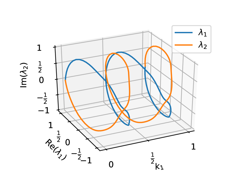
(a) Eigenvalues winding in opposite directions

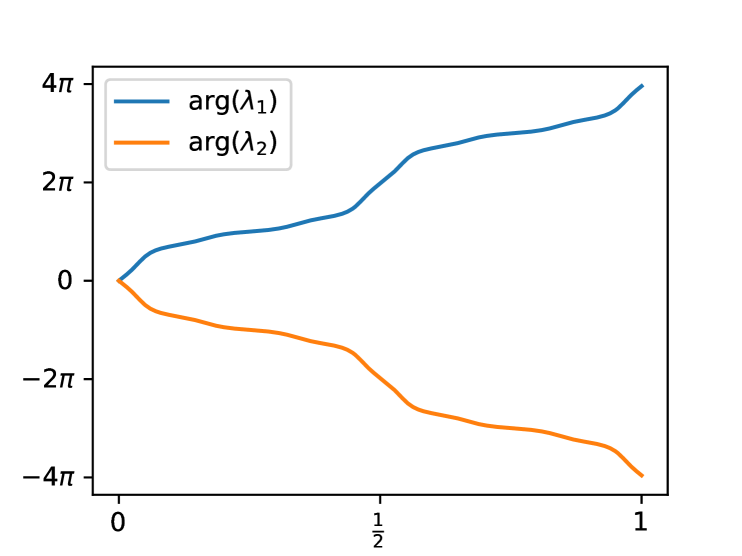
(b) Phase of the eigenvalues, corrected for continuity

Figure 1: Eigenvalues of the obstruction for the Kane-Mele model

A similar method, proposed in [CM17], is to introduce a small perturbation in order to avoid eigenvalue crossings, which makes each winding number trivial, and look for a family of logarithms satisfying

$${V}(k)=\mathrm{e}^{{L}_{1}(k)}\mathrm{e}^{{L}_{2}(k)}\dots\mathrm{e}^{{L}_{N}(k)},$$

where ${L}_{i}(s),\;i\in 1\dots N$ are anti-Hermitian. However, small perturbations of eigenvalues can introduce large changes in the eigenvectors, and hence produce a continuous but irregular path, which makes this method algorithmically difficult to implement.

4.2 Column interpolation method

From the counter-example given in Example 1, we see that constructing a homotopy of unitary matrices based from their eigenvalues may fail, as these can wind. In our method, instead of contracting eigenvalues, we rather contract the columns of $V(k)$ one by one. Algebraically, this corresponds to exploiting the fibration

$${\rm U}(N-1)\to{\rm U}(N)\to\SS^{2N-1},$$

which was suggested (but not explored further) in [FMP16a, p.81].

let ${\mathbb{T}}^{1}\ni k\mapsto V(k)\in{\rm U}(N)$ be a smooth map. We write $V(k)=(v_{1}(k),\ldots,v_{N}(k))$ where $v_{n}(k)\in\SS^{2N-1}$ is the $n$-th column of $V(k)$. Our strategy is to first contract the columns $v_{n}(k)$ iteratively to a fixed column $\underline{v_{n}}$, ensuring that they stay orthonormal, and then homotopise $\underline{V}=(\underline{v_{1}},\ldots,\underline{v_{N}})$ to the identity.

Let us assume that at step $1\leq n\leq N$, we have found how to contract the first $n-1$ columns to some fixed vectors: we have constructed $n-1$ smooth maps of orthonormal vectors $v_{1}(k,t),\ldots,v_{n-1}(k,t)$ such that $v_{j}(k,t=0)=v_{j}(k)$ and $v_{j}(k,t=1)=\underline{v_{j}}$. We denote by

$$P_{n-1}(k,t):=\mathbb{I}_{N}-\sum_{j=1}^{n-1}|v_{j}(k,t)\rangle\langle v_{j}(k,t)|,$$

the projection on the orthogonal of this family, of rank $N-n+1$. By hypothesis, at $t=1$, the projectors $P_{n-1}(k,t=1)$ are equal to a constant projector $\underline{P_{n-1}}$.

We now contract the $n$-th column $v_{n}(k,t)$ to a fixed column $\underline{v_{n}}\in{\rm Ran}\,\underline{P_{n-1}}$ while satisfying $v_{n}(k,t)\in{\rm Ran}\,P_{n-1}(k,t)$ for all $k,t\in{\mathbb{T}}^{1}\cup[0,1]$. This ensures that the constructed map for the $n$-th column is orthogonal to the previously constructed ones. First, for all fixed $k\in{\mathbb{T}}^{1}$, we parallel transport the orthogonal family $(v_{n}(k),\cdots,v_{N}(k))$ with respect to $P_{n-1}(k,\cdot)$, and obtain a smooth family of orthonormal frames $(\widetilde{v_{n}}(k,t),\cdots,\widetilde{v_{N}}(k,t))$ for $k,t\in{\mathbb{T}}^{1}\times[0,1]$. At this point, $\widetilde{v_{n}}(k,t=1)$ forms a non-trivial loop in ${\rm Ran}\,\underline{P_{n-1}}$. We now contract this to a single vector $\underline{v_{n}}$, distinguishing two cases, depending on whether $\widetilde{v_{n}}(k,t=1)$ can or cannot cover the whole of the unit sphere in ${\rm Ran}\,\underline{P_{n-1}}$.

Case $n<N$.

When $n<N$, the unit sphere in ${\rm Ran}\,\underline{P_{n-1}}$ is a manifold of real dimension $2(N-n)+1\geq 3$. The family $\left\{\widetilde{v_{n}}(k,t=1)\right\}_{k\in{\mathbb{T}}^{1}}$ describes a piecewise smooth loop on that manifold, and from Sard’s lemma it follows that there exists a vector $\underline{v_{n}}\in\SS^{2N-1}\cap{\rm Ran}\,\underline{P_{n-1}}$ such that $-\underline{v_{n}}$ does not belong to the loop $\left\{\widetilde{v_{n}}(k,t=1)\right\}_{k\in{\mathbb{T}}^{1}}$ (see Remark 3).

For all $k\in{\mathbb{T}}^{1}$, the family $(\widetilde{v_{n}}(k,1),\cdots,\widetilde{v_{N}}(k,1))$ is a basis of $\underline{P_{n-1}}$, so there exist (smooth) coefficients $c(k):=(c_{n}(k),\ldots,c_{N}(k))\in{\mathbb{C}}^{N-n+1}$ with $|c(k)|=1$ such that

$$\forall k\in{\mathbb{T}}^{1},\quad\underline{v_{n}}=\sum_{j=n}^{N}c_{j}(k)\widetilde{v_{j}}(k,1).$$

The map ${\mathbb{T}}^{1}\ni k\mapsto c(k)$ is a loop on the sphere $\SS^{2(N-n)+1}$. In addition, since $-\underline{v_{n}}$ never touches the loop $\left\{\widetilde{v_{n}}(k,t=1)\right\}_{k\in{\mathbb{T}}^{1}}$, $c(k)$ never touches the vector $-e_{1}:=(-1,0,\cdots,0)$. We can therefore contract the loop $c(k)$ to $e_{1}$ on $\SS^{2(N-n)+1}$ with the explicit contraction

$$c(k,t):=\dfrac{(1-t)c(k)+te_{1}}{\|(1-s)c(k)+te_{1}\|},$$ (7)

which is a well-defined smooth map from ${\mathbb{T}}^{1}\times[0,1]$ to $\SS^{2(N-n)+1}$. This contraction of coefficients directly translates into a contraction of $v_{n}(k)$ to $\underline{v_{n}}$ by setting

$$v_{n}(k,t):=\sum_{j=n}^{N}c_{j}(k,t)\widetilde{v_{j}}(k,t).$$

By construction, $v_{n}(k,t)$ is a normalised vector which is orthogonal to $(v_{1}(k,t),\ldots,v_{n-1}(k,t))$ for all $k,t\in{\mathbb{T}}^{1}\times[0,1]$. This concludes the construction in this case.

Remark 3.

In practice, in order to find numerically $\underline{v_{n}}$, we draw several random or well-chosen points $p_{j}\in\SS^{2N-1}$, which we project on $\underline{P_{n-1}}$ and normalise. We then pick

$$\underline{v_{n}}:=\operatorname*{arg\,max}_{j}\min_{k\in{\mathbb{T}}^{1}}\|\widetilde{v_{n}}(k,1)+p_{j}\|.$$

This ensures that the denominator in (7) is not too close to zero.

Case $n=N$.

For the last vector, i.e. when $n=N$, the previous construction can fail because $\widetilde{v_{N}}(k,t=1)$ can cover the whole of the unit sphere in ${\rm Ran}\,\underline{P_{n-1}}$. We therefore follow a different route. For all $k\in{\mathbb{T}}^{1}$, the vector $\widetilde{v_{N}}(k,t=1)$ always lies in the same one-dimensional subspace. In particular, there is a smooth phase $\phi:[0,1]\to{\mathbb{R}}$ so that

$$\forall k\in[0,1],\quad\widetilde{v_{N}}(k)=\underline{v_{N}}{\mathrm{e}}^{{\mathrm{i}}\phi(k)}\quad\text{with}\quad\underline{v_{N}}:=\widetilde{v_{N}}(0)\quad\text{(for instance)}.$$

By periodicity, one must have $\phi(1)=\phi(0)+2\pi m$ with $m\in{\mathbb{Z}}$. This gives

$$m =\frac{1}{2\pi}\left(\phi(1)-\phi(0)\right)=\dfrac{1}{2\pi}\int_{0}^{1}\phi^{\prime}(k){\mathrm{d}}k=\dfrac{1}{2\pi{\mathrm{i}}}\int_{0}^{1}\left\langle\widetilde{v_{N}}(k),\frac{{\mathrm{d}}}{{\mathrm{d}}k}\widetilde{v_{N}}(k)\right\rangle{\mathrm{d}}k.$$

We set $\widetilde{V}(k,t):=(v_{1}(k,t),\ldots v_{N-1}(k,t),\widetilde{v_{N}}(k,t))\in{\rm U}(N)$. This is a smooth deformation between $V(k)$ at $t=0$ and $\widetilde{V}(k,1)=(\underline{v_{1}},\ldots\underline{v_{N-1}},\widetilde{v_{N}}(k,1))$ at $t=1$. Also, we have

$$\left\langle\widetilde{v_{N}}(k),\frac{{\mathrm{d}}}{{\mathrm{d}}k}\widetilde{v_{N}}(k)\right\rangle=\Tr\left(\widetilde{V}(k,1)^{*}\frac{{\mathrm{d}}}{{\mathrm{d}}k}\widetilde{V}(k,1)\right){\mathrm{d}}k.$$

This leads to

$$m=\dfrac{1}{2\pi{\mathrm{i}}}\int_{0}^{1}\Tr\left(\widetilde{V}(k,1)^{*}\frac{{\mathrm{d}}}{{\mathrm{d}}k}\widetilde{V}(k,1)\right){\mathrm{d}}k=W\left(\det\widetilde{V}(\cdot,1)\right)=W(\det V(\cdot)),$$ (8)

where we recall that $W(\cdot)$ was defined in (6), and where we used the fact that the winding number is not affected by a smooth deformation: $W\left(\widetilde{V}(\cdot,t)\right)$ does not depend on $t$. We conclude that can contract the vector $\widetilde{v_{N}}$ to $\underline{v_{N}}$ if and only if $m=0$, or equivalently if $W(\det V)=0$. In this case, an explicit contraction is given by

$$v_{N}(k,t)=\widetilde{v_{N}}(k,t){\mathrm{e}}^{-{\mathrm{i}}t\phi(k)}.$$

Last step.

At this point, we have algorithmically constructed a smooth map ${\mathbb{T}}^{1}\times[0,1]\ni(k,t)\mapsto V(k,t)\in{\rm U}(N)$ such that $V(k,t=0)=V(k)$ and $V(k,t=1)=\underline{V}:=(\underline{v_{1}},\cdots,\underline{v_{N}})$. To get a contraction to the identity matrix ${\mathbb{I}}_{N}$, we write $\underline{V}=\exp(\underline{L})$, where $\underline{L}$ is anti-hermitian, and we take as our final homotopy

$$(k,t)\mapsto V(k,t){\mathrm{e}}^{-t\underline{L}}.$$

This concludes our constructive proof for Proposition 1.

Remark 4.

In our algorithm, we have tried to make the homotopy as smooth as possible. This means that we avoid composing homotopies sequentially, which is inefficient numerically, and that we wish that the method reduces to the logarithm method in the case where $V(k)$ is constant (where we know that the logarithm gives the geodesic in ${\rm U}(N)$ and therefore the most efficient path). If that is not a concern, then a simpler version of the algorithm can be given. After the first column is homotopised to a column $\underline{v_{1}}$, this vector can further be deformed to $e_{1}$, and therefore we can assume that $\underline{v_{1}}=e_{1}$. This implies that the homotopy $\widetilde{V}(k,t):=(v_{1}(k,t),\widetilde{v_{2}}(k,t),\ldots,\widetilde{v_{N}}(k,t)))$ satisfies $V(k,0)=V(k)$ and

$$\widetilde{V}(k,1)=\begin{pmatrix}1&\widetilde{v_{1,2}}(k,1)&\cdots&\widetilde{v_{1,N}}(k,1)\\ 0&\widetilde{v_{2,2}}(k,1)&\cdots&\widetilde{v_{2,N}}(k,1)\\ \vdots&\vdots&\cdots&\vdots\\ 0&\widetilde{v_{2,N}}(k,1)&\cdots&\widetilde{v_{N,N}}(k,1)\end{pmatrix}=:\begin{pmatrix}1&0\\ 0&V_{1}(k)\end{pmatrix},$$

where we used the fact that $\widetilde{V}(k,1)$ is unitary, so that $\widetilde{v_{1,2}}(k,1)=\cdots=\widetilde{v_{1,N}}(k,1)=0$. We have reduced the homotopy problem in ${\rm U}(N)$ to the homotopy problem in ${\rm U}(N-1)$, and therefore solve the problem by induction on $N$, using the case $n=N$ above to treat the base step.

Remark 5 (Parallelisability of the sphere).

In the case $N=2$, we can use the identification of ${\rm SU}(2)$ with $\SS(3)$ given by

$$\begin{pmatrix}a&-b^{*}\\ b&a^{*}\end{pmatrix}\mapsto\begin{pmatrix}a\\ b\end{pmatrix}$$

to simplify the algorithm, as done in [FMP16a]. More generally, if given a vector $x\in\{z\in{\mathbb{C}}^{N},|z|=1\}$ we had a systematic way to build an orthogonal basis of the (complex-)orthogonal $x^{\perp}$ in a way that is smooth with respect to $x$, we could exploit that in our algorithm. This is easily achieved in dimension $2$ by the mapping $(a,b)\mapsto(-b^{*},a^{*})$. However, this is impossible when $N=3$ (because this would imply the parallelisability of the $5$-dimensional sphere, which is false). We therefore have to follow a different route, using parallel transport to build this basis incrementally.

4.2.1 Extension for $2$-homotopies

We now consider the case of $2$-homotopies, and we want to contract a map ${\mathbb{T}}^{2}\ni(k_{1},k_{2})\mapsto V(k_{1},k_{2})\in{\rm U}(N)$. Following the same iterations as in the previous section, we see that at step $n<N$, the $n$-th column $\widetilde{v}(k_{1},k_{2},t=1)$ defines a $2$-dimensional sub-manifold on $\SS^{2N-1}\cap{\rm Ran}\,\underline{P_{n-1}}$ of dimension $2(N-n)+1\geq 3$, and we can find $\underline{v_{n}}$ so that $\underline{v_{n}}$ does not belong to this sub-manifold. We then follow the same steps.

For the last step $n=N$, there is a smooth phase function ${\mathbb{T}}^{2}\ni(k_{1},k_{2})\mapsto\phi(k_{1},k_{2})$ such that

$$\forall k_{1},k_{2}\in[0,1]^{2},\quad\widetilde{v_{N}}(k_{1},k_{2},1)=\underline{v_{N}}\exp({\mathrm{i}}\phi(k_{1},k_{2}))\quad\text{with}\quad\underline{v_{N}}:=\widetilde{v_{N}}(0,0,1)\quad\text{for instance}.$$

By periodicity and continuity, there is $m_{1},m_{2}\in{\mathbb{Z}}$ such that $\phi(k_{1}+1,k_{2})=\phi(k_{1},k_{2})+2\pi m_{1}$ and $\phi(k_{1},k_{2}+1)=\phi(k_{1},k_{2})+2\pi m_{2}$. As in (8), we find

$$\forall k_{2}\in{\mathbb{T}}^{1},\quad m_{1}=W(\det V(\cdot,k_{2}))\quad\text{and}\quad\forall k_{2}\in{\mathbb{T}}^{1},\quad m_{2}=W(\det V(k_{1},\cdot)).$$

If both number vanish, then a contraction is given by $v_{n}(k_{1},k_{2},t):=\widetilde{v_{n}}(k_{1},k_{2},t)\exp(-{\mathrm{i}}t\phi(k_{1},k_{2}))$. The constructive proof of Proposition 2 follows.

Remark 6.

This proof fails for $3$-homotopies. The reason is that with $N=2$, the first vector of ${\mathbb{T}}^{3}\ni(k_{1},k_{2},t_{3})\mapsto V(k_{1},k_{2},t_{3})\in{\rm U}(2)$ is now a $3$-dimensional sub-manifold in $\SS^{3}$, hence can wrap the whole sphere $\SS^{3}$. This is a manifestation of the second Chern class.

5 Numerical results

In this section, we apply the constructive method outlined above to the case of the Kane-Mele model ($d=2$), and silicon ($d=3$). We discretise the Brillouin zone with equispaced points (the Monkhorst-Pack grid). At each discrete point $k$, we diagonalise $H(k)$ and obtain the eigenvectors $(u_{n,k})_{1\leq n\leq N}$ corresponding to the $N$ lowest eigenvalues of $H(k)$. We then seek a unitary matrix $U_{m,n}(k)$ that makes $u^{\prime}_{n}(k)=\sum_{1\leq m\leq N}u_{mk}U_{mn}(k)$ as smooth as possible. The quantities needed by our algorithm are the overlaps $\langle u_{mk},u_{n,k+b}\rangle$ between neighbouring points $k$ and $k+b$, similar to other methods such as Wannier90 [MYP⁺14]. More information on this methodology can be found in [CLPS17].

5.1 The Kane-Mele model

The Kane-Mele model, first proposed in [KM05], is a toy model of a $\mathbb{Z}^{2}$ topological insulator. It is a tight-binding model on a 2D hexagonal lattice, with four degrees of freedom per site (two orbitals and two spins), two of which are occupied ($H(k)$ is a $4\times 4$ matrix, and $N=2$).

5.1.1 Description of the model

The Bloch representation of this model can be written as follows.

$$H_{k}=\sum_{a=1}^{5}d_{a}({k})\Gamma^{a}+\sum_{a,b=1\atop a<b}^{5}d_{ab}({k})\Gamma^{ab},$$ (9)

where $\Gamma^{ab}:=\frac{1}{2{\mathrm{i}}}[\Gamma^{a},\Gamma^{b}]$, and $\Gamma^{a}$ are the Dirac matrices $(\sigma^{x}\otimes{\mathbb{I}}_{N},\sigma^{z}\otimes{\mathbb{I}}_{N},\sigma^{y}\otimes{s}^{x},\sigma^{y}\otimes{s}^{y},\sigma^{y}\otimes{s}^{z})$, $\sigma^{j}$ and ${s}^{j}$ being the Pauli matrices of sublattice and spin respectively.

The functions $d_{a}(k)$ and $d_{ab}(k)$ in (9) are chosen as in [KM05]. In particular, $d_{a}$ is even and $d_{ab}$ odd, and the model satisfies a fermionic time-reversal symmetry. The model has $4$ free parameters: $t$, $\lambda_{S0}$, $\lambda_{\nu}$ and $\lambda_{R}$. Here, we fix the parameters $t=1,\lambda_{SO}=1$, and only vary $\lambda_{\nu}$ and $\lambda_{R}<2\sqrt{3}$. For every value of $\lambda_{R}<2\sqrt{3}$, the system undergoes a phase transition at the critical value $\lambda_{\nu}=3\sqrt{3}\approx 5.2$:

• For $\lambda_{\nu}>3\sqrt{3}$, the material is in a regular insulating phase.

• For $\lambda_{\nu}=3\sqrt{3}$, the material is in a transitional metallic phase: the gap closes, which means that the material is conducting.

• For $\lambda_{\nu}<3\sqrt{3}$, the material is in the Quantum Spin Hall (QSH) phase.

5.1.2 Numerical construction of Wannier functions for the Kane-Mele model

In order to construct localised Wannier functions for the Kane-Mele model, one needs to provide a Bloch frame that is regular enough on the Brillouin zone. In the QSH phase, no continuous and symmetric frame exists, but since the Chern number is trivial for any time-reversal symmetric Bloch bundle, there exists a non-symmetric continuous frame. Moreover, in this case, the eigenvalues of the obstruction have a non-trivial winding number, so the logarithm method of [CLPS17] cannot provide a homotopy of the obstruction.

In this section, we use the algorithm described above to construct a continuous initial guess of the Bloch frame, which can then be refined to a more regular one by a smoothing method, thus providing a well-localised Wannier function. The Brillouin zone was discretised with a $200\times 200$ grid. In the topologically trivial case, both methods produce a reasonable output (Figures 2(a) and 2(b)).

In order to measure localisation, we follow [MV97], and measure the spread of the Wannier functions $\Omega$. We also measure the quantity $\|\nabla_{k}u_{k}\|$, estimated using finite differences. Localised Wannier functions correspond to smooth gauge, and singularities in this quantity is therefore a sign of delocalisation.

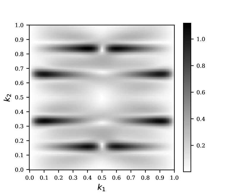
(a) Logarithm interpolation

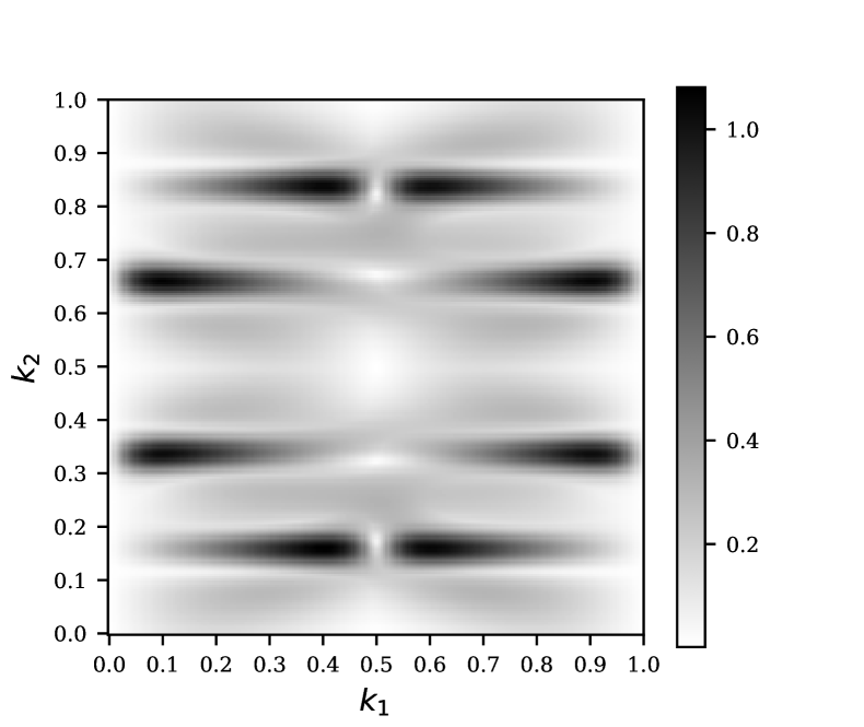
(b) Column interpolation

Figure 2: Local regularity $\|\nabla_{k}{u}\|$, $\lambda_{\nu}=6$ and $\lambda_{R}=1$ (regular insulating phase).

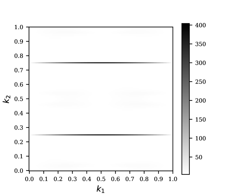
(a) Logarithm interpolation

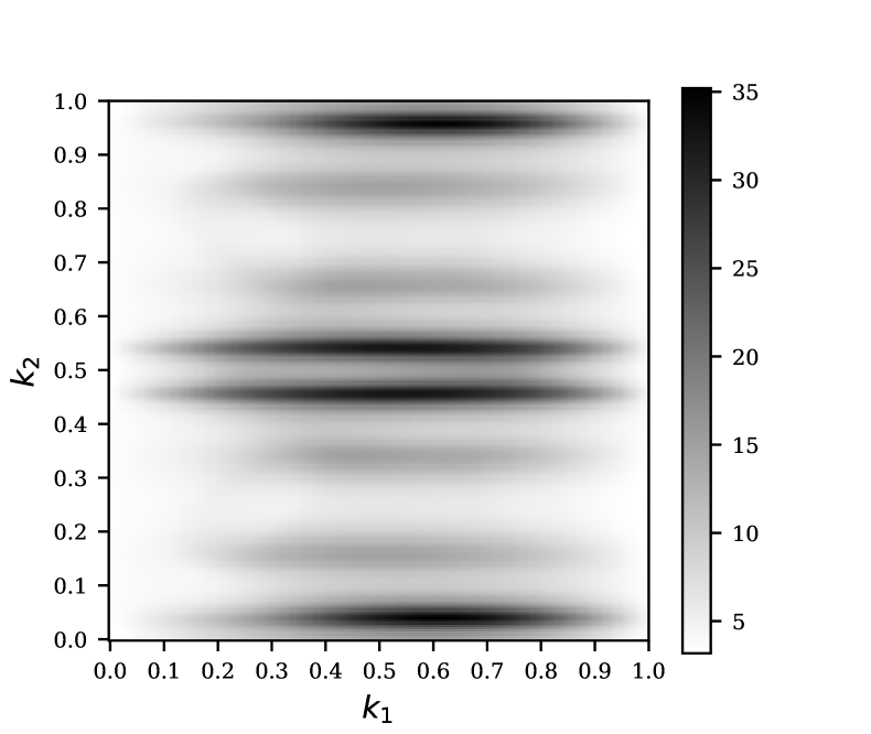
(b) Column interpolation

Figure 3: Local regularity $\|\nabla_{k}{u}\|$, $\lambda_{\nu}=0$ and $\lambda_{R}=1$ (QSH phase).

In Figure 3(a), the log interpolation method fails at constructing a continuous map in the topologically non-trivial QSH phase, as the measure of regularity $\|\nabla_{k}{u}\|$ exhibits lines of discontinuity, with very high maximal values. In contrast, in Figure 3(b), the column interpolation produces a smoother output, which also yields a lower maximal value of the regularity $\|\nabla_{k}{u}\|$.

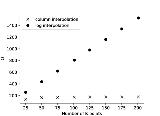
Figure 4: Convergence of $\Omega$ obtained by both methods, in the QSH phase ($\lambda_{\nu}=0,\lambda_{R}=1$)

The (dis)continuity of the resulting Bloch frame after each method is further demonstrated by the convergence with respect to ${k}$ point discretisation, displayed in Figure 4. In the log interpolation method, the discrete Bloch frames converge to a discontinuous one, as we see from the divergence of the norm of the gradient (estimated with finite differences). In contrast, the column interpolation produces a frame that has a smooth limit.

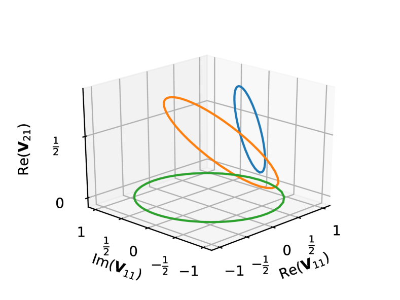
(a) $\lambda_{\nu}=1,\lambda_{R}=0$

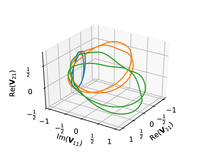
(b) $\lambda_{\nu}=1,\lambda_{R}=1$

Figure 5: Contraction of the first column of the obstruction, with the initial path in green ($k_{2}=1$) being deformed to a single point (yellow at $k_{2}=\frac{2}{3}$ then blue at $k_{2}=\frac{1}{3}$).

Figures 5(a) and 5(b) display selected components of $k_{1}\mapsto{V}_{\rm obs}(k_{1},k_{2})$ for $k_{2}=1,\frac{2}{3},\frac{1}{3}$. In Figure 5(a), we see how the obstruction path is contracted into the null path by our algorithm, in the QSH phase, with no Rashba term. In this case, the system decomposes into two independent copies of the Haldane model, one for each spin, which implies that the obstruction matrix is diagonal. This explains that the obstruction (the largest path in the plot) is horizontal, since ${V}_{21}=0$. Notice also that the diagonality of the obstruction, as well as time reversal symmetry, implying that ${k}\mapsto{\rm Re}\,V_{21}({k})$ is odd (which is verified up to rounding errors in the horizontal path), is broken by the method, as expected.

In Figure 5(b), for a Rashba term $\lambda_{R}=1$, the obstruction (the largest path, in green) is no longer diagonal (it has non-zero off-diagonal elements), but it still satisfies time-reversal symmetry, since ${k}\mapsto{\rm Re}\,V_{21}({k})$ is odd. The method breaks time-reversal symmetry to construct the continuous interpolation to the trivial path.

5.2 Numerical results for Silicon

Using Quantum Espresso, [GSB⁺09], the Bloch waves of Silicon for various discretisations of the Brillouin zone were provided to the homotopy constructing methods, in order to compare the numerical results of our column interpolation algorithm with the ones provided by the logarithm method of [CLPS17].

Table 1: Value of the Marzari-Vanderbilt localisation functional $\Omega$ (in Bohr²) for frames on various discretisations of the Brillouin zone

Discretisation of the BZ	$5\times 5\times 5$	$10\times 10\times 10$	$15\times 15\times 15$	$20\times 20\times 20$
After logarithm method	25.72	29.70	30.62	30.94
After column interpolation	40.88	35.31	53.68	46.80
After MV optimisation
(log initial guess)	19.30	22.06	22.71	22.95
After MV optimisation
(col initial guess)	19.30	22.06	22.71	22.95

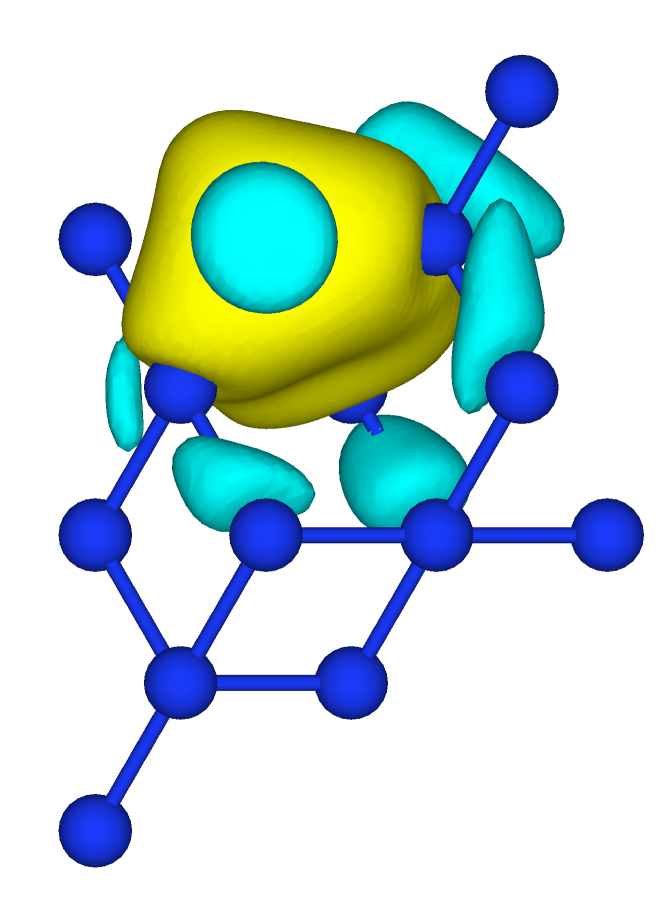
(a) Logarithm method

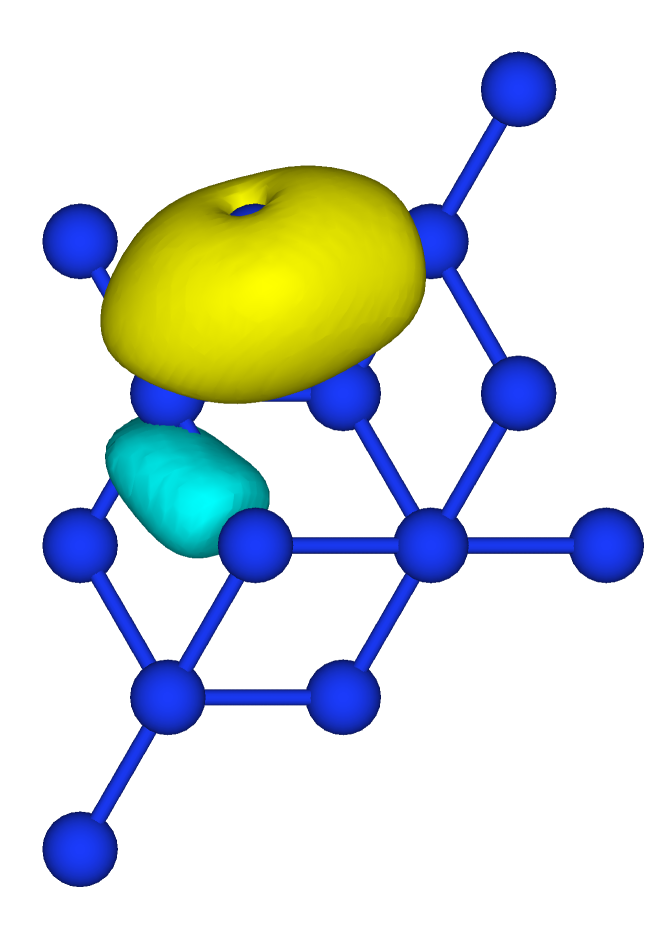
(b) Column interpolation method

Figure 6: One of the four Wannier functions of silicon, isosurface plot at $20\%$ of maximal value.

In Table 1, we can see that the value of the localisation functional $\Omega$ is better for the logarithm method than for ours, but, after optimisation of the Marzari-Vanderbilt procedure [MMY⁺12], both methods agree.

In Figure 6, we display some Wannier functions computed by both methods, before optimisation. The representation was done through Wannier90 [MYP⁺14] and VESTA [MI11]. The localisation of both is not optimal, which is expected, but the Wannier functions are still localised, and physically relevant.

Conclusion

We presented a new method to construct localised Wannier functions. It is proven to work even in the case of topological insulators which causes most published algorithms to fail. In the “easy” cases, it works similarly to the method of [CLPS17]. As that method, it only localises Wannier functions across unit cells, and does not attempt to localise the functions inside the unit cell. This is problematic in the case of large unit cells, which is the case of many real topological insulators. The efficient numerical construction of Wannier functions in these cases remains therefore an open problem.

(D. Gontier)	Université Paris-Dauphine, PSL Research University, CEREMADE
	75775 Paris, France
	E-mail address: gontier@ceremade.dauphine.fr
(A. Levitt)	Inria Paris and Université Paris-Est, CERMICS (ENPC)
	F-75589 Paris Cedex 12, France
	E-mail address: antoine.levitt@inria.fr
(S. Siraj-Dine)	Université Paris-Est, CERMICS (ENPC) and Inria Paris
	F-77455 Marne-la-Vallée, France
	E-mail address: sami.siraj-dine@enpc.fr

The PhD of Sami Siraj-Dine is supported by the Labex Bézout.

References

- [BPC+07] C. Brouder, G. Panati, M. Calandra, C. Mourougane, and N. Marzari. Exponential Localization of Wannier Functions in Insulators. Phys. Rev. Lett., 98(4), 2007.
- [CHN16] H.D. Cornean, I. Herbst, and Gh. Nenciu. On the construction of composite Wannier functions. Ann. Henri Poincaré, 17(12):3361–3398, 2016.
- [CLPS17] É. Cancès, A. Levitt, G. Panati, and G. Stoltz. Robust determination of maximally localized Wannier functions. Phys. Rev. B, 95(7):075114, 2017.
- [CM17] H.D. Cornean and D. Monaco. On the construction of Wannier functions in topological insulators: the 3D case. Ann. Henri Poincaré, 18:3863–3902, 2017.
- [DLY15] A. Damle, L. Lin, and L. Ying. Compressed representation of kohn–sham orbitals via selected columns of the density matrix. J. Chem. Theory Comput., 11(4):1463–1469, 2015.
- [DLY17] A. Damle, L. Lin, and L. Ying. Scdm-k: Localized orbitals for solids via selected columns of the density matrix. J. Comput. Phys., 334:1–15, 2017.
- [FKM07] L. Fu, Ch.L. Kane, and E.J. Mele. Topological insulators in three dimensions. Phys. Rev. Lett., 98(10):106803, 2007.
- [FMP16a] D. Fiorenza, D. Monaco, and G. Panati. Construction of real-valued localized composite Wannier functions for insulators. Ann. Henri Poincaré, 17(1):63–97, 2016.
- [FMP16b] D. Fiorenza, D. Monaco, and G. Panati. invariants of topological insulators as geometric obstructions. Comm. Math. Phys., 343(3):1115–1157, 2016.
- [GSB+09] P. Giannozzi, Baroni S., S. Bonini, Matteo Calandra, Roberto Car, Carlo Cavazzoni, Davide Ceresoli, Guido L Chiarotti, Matteo Cococcioni, Ismaila Dabo, Andrea Dal Corso, Stefano de Gironcoli, Stefano Fabris, Guido Fratesi, Ralph Gebauer, Uwe Gerstmann, Christos Gougoussis, Anton Kokalj, Michele Lazzeri, Layla Martin-Samos, Nicola Marzari, Francesco Mauri, Riccardo Mazzarello, Stefano Paolini, Alfredo Pasquarello, Lorenzo Paulatto, Carlo Sbraccia, Sandro Scandolo, Gabriele Sclauzero, Ari P Seitsonen, Alexander Smogunov, Paolo Umari, and Renata M Wentzcovitch. Quantum espresso: a modular and open-source software project for quantum simulations of materials. J. Phys. Condens. Matter, 21(39):395502, 2009.
- [Hal88] F.D.M. Haldane. Model for a quantum hall effect without landau levels: Condensed-matter realization of the” parity anomaly”. Phys. Rev. Lett., 61(18):2015, 1988.
- [KM05] C.L. Kane and E.J. Mele. topological order and the quantum spin Hall effect. Phys. Rev. Lett., 95:146802, 2005.
- [KSV93] R.D. King-Smith and D. Vanderbilt. Theory of polarization of crystalline solids. Phys. Rev. B, 47(3):1651, 1993.
- [Lin18] L. Lin. Private communication, 2018.
- [MCCL15] J.I. Mustafa, S. Coh, M.L. Cohen, and S.G. Louie. Automated construction of maximally localized wannier functions: Optimized projection functions method. Phys. Rev. B, 92(16):165134, 2015.
- [MCCL16] J.I. Mustafa, S. Coh, M.L Cohen, and S.G. Louie. Automated construction of maximally localized Wannier functions for bands with nontrivial topology. Physical Review B, 94(12):125151, 2016.
- [MI11] K. Momma and F. Izumi. VESTA3 for three-dimensional visualization of crystal, volumetric and morphology data. J. Appl. Crystallogr., 44(6):1272–1276, 2011.
- [MMY+12] N. Marzari, A.A. Mostofi, J.R. Yates, I. Souza, and D. Vanderbilt. Maximally localized Wannier functions: Theory and applications. Rev. Mod. Phys., 84(4):1419, 2012.
- [MV97] N. Marzari and D. Vanderbilt. Maximally localized generalized wannier functions for composite energy bands. Phys. Rev. B, 56:12847–12865, 1997.
- [MYP+14] A.A. Mostofi, J.R. Yates, Giovanni Pizzi, Young-Su Lee, Ivo Souza, David Vanderbilt, and Nicola Marzari. An updated version of wannier90: A tool for obtaining maximally-localised wannier functions. Comput. Phys. Commun., 185(8):2309–2310, 2014.
- [Nen83] G. Nenciu. Existence of the exponentially localised Wannier functions. Comm. Math. Phys., 91(1):81–85, 1983.
- [Pan07] G. Panati. Triviality of Bloch and Bloch–Dirac bundles. Ann. Henri Poincaré, 8(5):995–1011, 2007.
- [PP13] G. Panati and A. Pisante. Bloch bundles, Marzari-Vanderbilt functional and maximally localized Wannier functions. Comm. Math. Phys., 322:835–875, 2013.
- [RS78] M. Reed and B. Simon. IV: Analysis of Operators. Elsevier, 1978.
- [SV11] A.A. Soluyanov and D. Vanderbilt. Wannier representation of topological insulators. Phys. Rev. B, 83:035108, 2011.
- [SV12] A.A. Soluyanov and D. Vanderbilt. Smooth gauge for topological insulators. Phys. Rev. B, 85:115415, 2012.
- [WSC09] X. Wu, A. Selloni, and R. Car. Order-n implementation of exact exchange in extended insulating systems. Phys. Rev. B, 79(8):085102, 2009.
- [WST16] G.W. Winkler, A.A. Soluyanov, and M. Troyer. Smooth gauge and wannier functions for topological band structures in arbitrary dimensions. Phys. Rev. B, 93:035453, 2016.