KEK Preprint 2018-81 CHIBA-EP-229 Confinement/deconfinement phase transition in SU(3) Yang-Mills theory and non-Abelian dual Meissner effect

Abstract:

The dual superconductivity is a promising mechanism of quark confinement. In the preceding works, we have given a non-Abelian dual superconductivity picture for quark confinement, and demonstrated the numerical evidences on the lattice.
In this talk, we focus on the the confinement and deconfinement phase transition at finite temperature in view of the dual superconductivity. By using our new formulation of lattice Yang-Mills theory and numerical simulations on the lattice, we extract the dominant mode for confinement by decomposing the Yang-Mills field, and we investigate the Polyakov loop average, static quark potential, chromoelectric flux, and induced monopole current for both Yang-Mills field and decomposed restricted field in both confinement and deconfinement phase at finite temperature. We further discuss the role of the chromomagnetic monopole in the confinement/deconfinement phase transition.

1 Introduction

The dual superconductivity is a promising mechanism for quark confinement [1]. To establish the dual superconductivity picture, we must show that magnetic monopoles play a dominant role in quark confinement. For this purpose, we have constructed a new framework for the $SU(N)$ Yang-Mills theory on the lattice, called the decomposition method, which gives the decomposition of a gauge link variable $U_{x,\mu}=X_{x,\mu}V_{x,\mu}$ to extract a variable $V_{x,\mu}$ called the restricted field as the dominant mode for quark confinement in the gauge independent way. (See [2] for a review.) This formulation can overcome criticism raised for the Abelian projection method [3] for extracting Abelian magnetic monopoles, i.e., the magnetic monopole is obtained only in special Abelian gauges such as the maximal Abelian (MA) gauge [4]. The Abelian projection is nothing but a gauge fixing to break the gauge symmetry, which breaks also the color symmetry (global symmetry).

In the new framework, the $SU(3)$ Yang-Mills theory has two options for choosing the fundamental field variables: the minimal and maximal options. These two options are discriminated by the maximal stability subgroup $\tilde{H}$ of the gauge group $SU(3)$. In the minimal option, the maximal stability group is a non-Abelian group $\tilde{H}=U(2)$ and the restricted field is used to extract non-Abelian magnetic monopoles. The minimal option is suggested from the non-Abelian Stokes theorem for the Wilson loop operator in the fundamental representation. In the preceding works, we have provided numerical evidences of the non-Abelian dual superconductivity using the minimal option for the $SU(3)$ Yang-Mills theory on a lattice. In the maximal option, the maximal stability group is an Abelian group $\tilde{H}=U(1)\times U(1)$, the maximal torus subgroup of $SU(3)$. This decomposition was first constructed by Cho and Faddeev and Niemi [5] by extending the Cho-Duan-Ge-Faddeev-Niemi (CDGFN) decomposition for the $SU(2)$ case [6], and is nothing but the gauge invariant extension of the Abelian projection in the maximal Abelian gauge. Therefore, the restricted field in the maximal option involves only the Abelian magnetic monopole.

In this talk, we investigate the confinement/deconfinement phase transition at finite temperature from a viewpoint of the dual superconductivity in the both minimal and maximal options. The preliminary results are given by preceding works [9][10]. For this purpose, we examine several quantities constructed by the restricted fields in both options as well as the original Yang-Mills field at finite temperature, e.g., the distribution and average of the Polyakov loops, the static potential from the Wilson loop, the dual Meissner effects, and so on. The the dual Meissner effects at finite temperature can be examined by measuring the distribution of the chromo-electric field strength (or chromo flux) generated from a pair of the static quark and antiquark and the associated magnetic-monopole current induced around it. In particular, we discuss the role of the non-Abelian magnetic monopole in confinement/deconfinement phase transition.

2 Gauge link decompositions

In this section, we give a brief review of the decomposition method, which enables one to extract the dominant mode for quark confinement in the $SU(N)$ Yang-Mills theory (see [2] in detail). We decompose the gauge link variable $U_{x,\mu}$ into the product of the two variables, $V_{x,\mu}$ and $X_{x,\mu}$, in such a way that the new variable $V_{x,\mu}$ is transformed by the full $SU(N)$ gauge transformation $\Omega_{x}$ as the gauge link variable $U_{x,\mu}$, while $X_{x,\mu}$ transforms as the site variable:

$$U_{x,\mu} =X_{x,\mu}V_{x,\mu}\in G=SU(N),$$ (1a)

$$U_{x,\mu} \longrightarrow U_{x,\nu}^{\prime}=\Omega_{x}U_{x,\mu}\Omega_{x+\mu}^{{\dagger}},V_{x,\mu}\longrightarrow V_{x,\nu}^{\prime}=\Omega_{x}V_{x,\mu}\Omega_{x+\mu}^{{\dagger}},\text{ \ }X_{x,\mu}\longrightarrow X_{x,\nu}^{\prime}=\Omega_{x}X_{x,\mu}\Omega_{x}^{{\dagger}}.$$ (1b)

From the physical point of view, $$V_{x,\mu} X_{x,\mu} SU(3)$$ could be the dominant mode for quark confinement, while is the remainder part. For the Yang-Mills theory, we have two possible options discriminated by the stability subgroup of the gauge group, which we call the minimal and maximal options.

2.1 Minimal option

The minimal option is obtained for the stability subgroup $\tilde{H}=U(2)=SU(2)\times U(1)$. By introducing a single color field, $\bm{h}_{x}=\xi_{x}\frac{\lambda^{8}}{2}\xi_{x}^{{\dagger}}\in Lie[SU(3)/U(2)]$, with $\lambda^{8}$ being the last diagonal Gell-Mann matrix and $\xi_{x}$ an $SU(3)$ group element, the decomposition is obtained by solving the defining equations:

$$D_{\mu}^{\epsilon}[V]\bm{h}_{x}:=\frac{1}{\epsilon}\left[V_{x,\mu}\bm{h}_{x+\mu}-\bm{h}_{x}V_{x,\mu}\right]=0\text{ }.$$ (2)

The defining equation can be solved exactly, and the solution is given by

$$X_{x,\mu} =\widehat{L}_{x,\mu}^{{\dagger}}\det(\widehat{L}_{x,\mu})^{1/3}g_{x}^{-1},\text{ \ }V_{x,\mu}=X_{x,\mu}^{{\dagger}}U_{x,\mu}=g_{x}\widehat{L}_{x,\mu}U_{x,\mu},$$ (3a)

$$\widehat{L}_{x,\mu} :=\left(L_{x,\mu}L_{x,\mu}^{{\dagger}}\right)^{-1/2}L_{x,\mu},\text{ \ \ }L_{x,\mu}:=\frac{5}{3}\mathbf{1}+\frac{2}{\sqrt{3}}(\bm{h}_{x}+U_{x,\mu}\bm{h}_{x+\mu}U_{x,\mu}^{{\dagger}})+8\bm{h}_{x}U_{x,\mu}\bm{h}_{x+\mu}U_{x,\mu}^{{\dagger}}.$$ (3b)

Here, the variable $$g_{x}:=e^{i2\pi q/3}\exp(-ia_{x}^{0}\bm{h}_{x}-i\sum\nolimits_{j=1}^{3}a_{x}^{(j)}\mathbf{u}_{x}^{(j)}) U(2) \mathbf{u}_{x}^{(j)} su(2) q g_{x}=\mathbf{1} D_{\mu}[\bm{V}]\bm{h}(x)=0 \mathrm{tr}(\bm{X}_{\mu}(x)\bm{h}(x)) =0$$ is the part which is undetermined from eq(2) alone, ’s are -Lie algebra valued, and   is an integer. Note that the above defining equation with corresponds to the continuum version: and . In the continuum limit, indeed, the decomposition in the continuum theory is reproduced.

The decomposition is uniquely obtained as the solution of the defining equation, once a set of color fields $\ \{\bm{h}_{x}\}$ are given. To determine the configuration of color fields, we use the reduction condition of minimizing the functional:

$$F_{\text{red}}[\bm{n}_{x}^{(8)}]=\sum_{x,\mu}\mathrm{tr}\left\{(D_{\mu}^{\epsilon}[U_{x,\mu}]\bm{h}_{x})^{{\dagger}}(D_{\mu}^{\epsilon}[U_{x,\mu}]\bm{h}_{x})\right\}.$$ (4)

2.2 Maximal option

The maximal option is obtained for the stability subgroup of the maximal torus subgroup of $G$: $\tilde{H}=U(1)\times U(1)$. By introducing the color field, $\bm{n}_{x}^{(3)}=\xi_{x}\frac{\lambda^{3}}{2}\xi_{x}^{{\dagger}}\in Lie[SU(3)/U(1)\times U(1)],\quad\ \bm{n}_{x}^{(8)}=\xi_{x}\frac{\lambda^{8}}{2}\xi_{x}^{{\dagger}}\in Lie[SU(3)/U(2)],$ with $\lambda^{3}$, $\lambda^{8}$ being the two diagonal Gell-Mann matrices and $\xi$ an $SU(3)$ group element, the decomposition is obtained by solving the defining equations:

$$D_{\mu}^{\epsilon}[V]\bm{n}_{x}^{(j)}:=\frac{1}{\epsilon}\left[V_{x,\mu}\bm{n}_{x+\mu}^{(j)}-\bm{n}_{x}^{(j)}V_{x,\mu}\right]=0\quad(j=3,8)\text{ .}$$ (5)

The defining equation can be solved exactly, and the solution is given by

$$X_{x,\mu} =\widehat{K}_{x,\mu}^{{\dagger}}\det(\widehat{K}_{x,\mu})^{1/3}g_{x}^{-1},\text{\ \ }V_{x,\mu}=X_{x,\mu}^{{\dagger}}U_{x,\mu},$$ (6a)

$$\widehat{K}_{x,\mu} :=\left(K_{x,\mu}K_{x,\mu}^{{\dagger}}\right)^{-1/2}K_{x,\mu},\text{ \ \ }K_{x,\mu}:=\mathbf{1}+6(\bm{n}_{x}^{(3)}U_{x,\mu}\bm{n}_{x+\mu}^{(3)}U_{x,\mu}^{{\dagger}})+6(\bm{n}_{x}^{(8)}U_{x,\mu}\bm{n}_{x+\mu}^{(8)}U_{x,\mu}^{{\dagger}}).$$ (6b)

Here, the variable $$g_{x}:=e^{i2\pi q/3}\exp(-ia_{x}^{3}\bm{n}_{x}^{(3)}-ia_{x}^{(8)}\bm{n}_{x}^{(8)}) q U(1)\times U(1) g_{x}=\mathbf{1} D_{\mu}[\bm{V}]\bm{n}^{(j)}(x)=0 \mathrm{tr}(\bm{X}_{\mu}(x)\bm{n}^{(j)}(x)) =0$$ with integer is the part which is undetermined from eq(5) alone. Note that the above defining equation with corresponds to the continuum version: and . In the continuum limit, we can reproduce the decomposition in the continuum theory.

The decomposition is uniquely obtained as the solution (7) of the defining equations, once a set of color fields $\left\{\bm{n}_{x}^{(3)},\bm{n}_{x}^{(8)}\right\}$ are given. To determine the configuration $\left\{\bm{n}_{x}^{(3)},\bm{n}_{x}^{(8)}\right\}$ of color fields, we use the reduction condition of minimizing the functional:

$$F_{\text{red}}[\bm{n}_{x}^{(3)},\bm{n}_{x}^{(8)}]=\sum_{x,\mu}\sum_{j=3,8}\mathrm{tr}\left\{(D_{\mu}^{\epsilon}[U_{x,\mu}]\bm{n}_{x}^{(j)})^{{\dagger}}(D_{\mu}^{\epsilon}[U_{x,\mu}]\bm{n}_{x}^{(j)})\right\}.$$ (7)

Note that, the resulting decomposition is the gauge-invariant extension of the Abelian projection in the maximal Abelian (MA) gauge.

3 Numerical simulations on the lattice

We set up the numerical simulations at finite temperature adopting the standard Wilson action with the inverse gauge coupling constant $\beta=2N_{c}/g^{2}$ ($N_{c}=3)$ and using the pseudo heat-bath algorithm and the over-relaxation algorithm to generate the gauge field configurations (link variables) $\{U_{x,\mu}\}$ on the lattice of size $N_{s}^{3}\times N_{T}$ . We prepare 1000 gauge configurations every 100 seeps with 8 over relaxations after 8000 thermalization sweeps with cold start for the fixed spatial size $N_{s}$ and the temporal size $N_{T}$: $N_{s}=24$, $N_{T}=6$, where the temperature varies by changing the coupling $\beta$ ($5.75\leq\beta\leq 6.50$).

We obtain the color field configurations for the minimal and maximal options by solving the reduction conditions, and then we perform the decomposition of the gauge link variable $U_{x,\mu}=X_{x,\mu}V_{x,\mu}$ by using the formula given in the previous section, i.e., for the minimal option eq(3)  with the color field$\ \{\bm{h}_{x}\}$ by minimizing eq(4), for the maximal option eq(6) and the color field $\left\{\bm{n}_{x}^{(3)},\bm{n}_{x}^{(8)}\right\}$ by minimizing eq(7). In the measurement of the Polyakov loop average and the Wilson loop average defined below, we apply the APE smearing technique [7] to reduce noises .

3.1 Polyakov-loop average at the confinement/deconfinement transition

First, we investigate the distribution of single Polyakov loops. For a set of the original gauge field configurations $\{U_{x,\mu}\}$ and the restricted gauge field configurations $\{V_{x,\mu}\}$ in the minimal and maximal options, we define the respective Polyakov loops by

$$P_{U}^{\mathrm{YM}}(\mathbf{x}):=\frac{1}{3}\text{{tr}}\left(P\prod\limits_{t=1}^{N_{T}}U_{(\mathbf{x},t),4}\right),\ P_{V}^{\min}(\mathbf{x}):=\frac{1}{3}\text{{tr}}\left(P\prod\limits_{t=1}^{N_{T}}V_{(\mathbf{x},t),4}^{(\min)}\right),\ P_{V}^{\max}(\mathbf{x}):=\frac{1}{3}\text{{tr}}\left(P\prod\limits_{t=1}^{N_{T}}V_{(\mathbf{x},t),4}^{(\max)}\right)\text{ ,}$$ (8)

and the space-averaged Polyakov loops by

$$P_{YM}:=\frac{1}{L^{3}}\sum_{\mathbf{x}}P_{U}^{\mathrm{YM}}(\mathbf{x}),\ \ \ P_{\min}:=\frac{1}{L^{3}}\sum_{\mathbf{x}}P_{V}^{\min}(\mathbf{x}),\ P_{\max}:=\frac{1}{L^{3}}\sum_{\mathbf{x}}P_{V}^{\max}(\mathbf{x}),$$ (9)

where the value of the Polyakov loop is averaged over the space volume for each configuration.

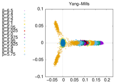
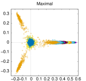
Figure 1: The distribution of the space-averaged Polyakov loop on the complex plane: (Left) Yang-Mills field (Middlel) restricted field in minimal option (Right) restricted field in maximal option.

Figure 1 shows the plots of and $\{P_{U}^{\mathrm{YM}}(\mathbf{x})\}$, $\{P_{V}^{\min}(\mathbf{x})\}$ and $\{P_{V}^{\max}(\mathbf{x})\}$ on the complex plane measured from a set of the original Yang-Mills field configurations and a set of the restricted field configurations in the minimal and maximal options, respectively. We find that the value of the space-averaged Polyakov loops are different option by option, but all the distributions on the complex plane equally reflect the expected center symmetry $Z(3)$ of the $SU(3)$ gauge group.

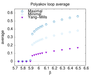
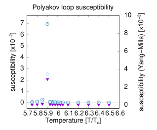
Figure 2: (Left) Polyakov-loop averages for the original field and the restricted field in the minimal and maximal options from bottom to top. (Right) The susceptibility of the Polyakov loop for the original field and the restricted field in the minimal and maximal options from bottom to top.

The left panel of Figure 2 shows the comparison of  three Polyakov-loop averages, i.e., $\left\langle P_{YM}\right\rangle$, $\left\langle P_{\min}\right\rangle$, and $\left\langle P_{\max}\right\rangle$, for various temperature ($\beta$), where the symbol $\left\langle\mathcal{O}\right\rangle$ denotes the average of the operator $\mathcal{O}$ over the ensemble of the configurations. The right panel of Fig. 2 shows their susceptibilities, $\chi:=\left\langle P_{\ast}^{2}\right\rangle-\left\langle P_{\ast}\right\rangle^{2}$, with $P_{\ast}$ being one of $P_{YM}$, $P_{\min}$, and $P_{\max}$. These panels clearly show that both the minimal and maximal options reproduce the critical point of the original Yang-Mills field theory. Thus, these three Polyakov-loop averages give the identical critical temperature, i.e., $\beta=5.9$.

3.2 Static quark–antiquark potential at finite temperature

Next, we investigate the static quark–antiquark potential at finite temperature. To obtain the static potential at finite temperature, we adopt the Wilson loop operator, (see the left panels of Fig.3), which is defined for the rectangular loop $C$ with the spatial length $R$ and the temporal length $\tau$ which is maximally extended in the temporal direction, i.e., $\tau=1/T$. According to the standard argument, for large $\tau$ i.e., small $T$, the static potential is obtained from the original gauge field $U$ and the restricted gauge field $V$:

$$V(R;U):=-\frac{1}{\tau}\log\left\langle W_{U}\right\rangle=-T\log\left\langle W_{U}\right\rangle,\quad V(R;V):=-\frac{1}{\tau}\log\left\langle W_{V}\right\rangle=-T\log\left\langle W_{V}\right\rangle.$$ (10)

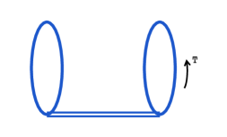
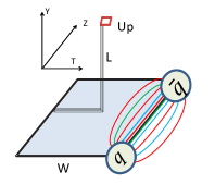
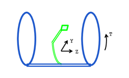
Figure 3: The set up for the measurement of the static quark-antiquark potential at finite temperature. (Left) the Wilson loop (Middle) The gauge-invariant operator $tr(WLU_{p}L)$ between a plaquette $U_{p}$ and the Wilson loop $W$. (Right) Measurement of the chromo-flux at finite temperature.

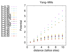
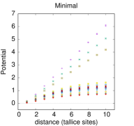
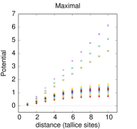
Figure 4: The static quark potential obtained using the maximally extended Wilson loop from the data set (II) at various temperatures $N_{T}=6$ and $5.75\leq\beta\leq 6.5$ (Left) original gauge field, (Middle) restricted field in the minimal option, (Right) restricted field in the maximal option. (applying APE smearing 8 times with weight 0.2)

Figure 4 shows the static potentials at various temperatures ($\beta$) calculated according to the definition (10). By comparing these results, we find that the potential is reproduced by the restricted field alone in both options. Therefore, we have shown the restricted $V$-field dominance for both options in the static potential at finite temperature.

3.3 Chromo-flux tube at finite temperature

We proceed to investigate the non-Abelian dual Meissner effect at finite temperature. For this purpose, we measure the chromo-flux created by a quark-antiquark pair, which is represented by the maximally extended Wilson loop $W$ as given in the middle and right panel of Fig.3. The chromo-field strength, i.e., the field strength of the chromo-flux created by the Wilson loop $W$ as the source, is measured by using a plaquette variable $U_{p}$ as the probe operator for the field strength. We use the gauge-invariant correlation function which is the same as that used at zero temperature [8]:

$$F_{\mu\nu}^{q\bar{q}}=\sqrt{\frac{\beta}{6}}\rho_{{}_{U_{P}}}\text{, \ \ \ }\rho_{{}_{U_{P}}}:=\frac{\left\langle\mathrm{tr}\left(WLU_{p}L^{{\dagger}}\right)\right\rangle}{\left\langle\mathrm{tr}\left(W\right)\right\rangle}-\frac{1}{N_{c}}\frac{\left\langle\mathrm{tr}\left(U_{p}\right)\mathrm{tr}\left(W\right)\right\rangle}{\left\langle\mathrm{tr}\left(W\right)\right\rangle}\text{ },$$ (11)

where $L$ is the Wilson line connecting the source $W$ and the probe $U_{p}$ to guarantee the gauge-invariance. Indeed, in the naive continuum limit, the connected correlator $\rho_{{}_{U_{P}}}$ reduces to $\rho_{{}_{U_{P}}}\overset{\varepsilon\rightarrow 0}{\simeq}g\epsilon^{2}\left\langle\mathcal{F}_{\mu\nu}\right\rangle_{q\bar{q}}:=\frac{\left\langle\mathrm{tr}\left(g\epsilon^{2}\mathcal{F}_{\mu\nu}L^{{\dagger}}WL\right)\right\rangle}{\left\langle\mathrm{tr}\left(W\right)\right\rangle}+O(\epsilon^{4})$.

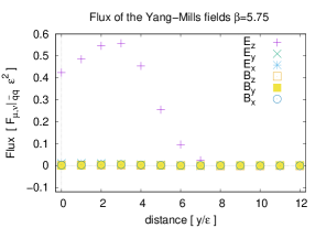
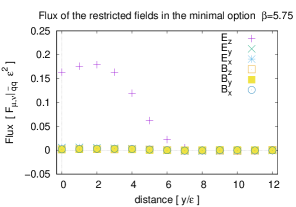
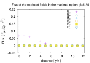
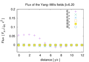
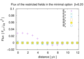
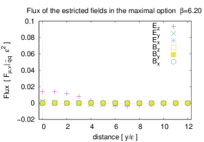
Figure 5: Measurement of chromo flux: $E_{x}=F^{q\bar{q}}_{14}$, $E_{y}=F^{q\bar{q}}_{24}$, $E_{Z}=F^{q\bar{q}}_{34}$, $B_{x}=F^{q\bar{q}}_{23}$, $B_{y}=F^{q\bar{q}}_{31}$, $B_{z}=F^{q\bar{q}}_{12}$ . The upper panels show the plots of chromo fluxes at a low temperature in the confiment phase ($T<T_{c}$), and the lower panels show those at a high temperature in the deconfinement phase .($T_{c}<T$). The left-column panels show the chromo flux for Yang-Mills field, and the middle- and right-column panels show the cheomo flux for the restricted field in the minimal and mxaimal options, respectively .

Figure 5 shows the chromo flux measured by using eq(11). At a low-temperature in the confinement phase, $T<T_{c}$, we observe that only the component $E_{z}$ of the chromoelectric flux tube in the direction connecting a quark and antiquark pair is non-vanishing, while the other components take vanishing values. (See the upper panels of Fig. 5. ) At a high-temperature in the deconfinement phase, $T>T_{c}$, we observe the non-vanishing component $E_{y}$ orthogonal to the chromoelectric flux, which means no more squeezing of the chromoelectric flux tube. (See the lower panels of Fig. 5 .) This is a numerical evidence for the disappearance of the dual Meissner effect in the high-temperature deconfinement phase.

3.4 Magnetic–monopole current and dual Meissner effect at finite temperature

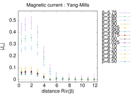
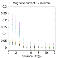
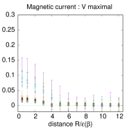
Figure 6: The magnitude $\sqrt{k_{\mu}k_{\mu}}$ of the induced magnetic current $k_{\mu}$ around the flux tube connecting the quark-antiquark pair as a function of the distance y from the z axis for various values of $\beta$ i.e., temperature. (Left) Yang-Mills filed (Middle) minimal option, (Right) maximal option.

Finally, we investigate the dual Meissner effect by measuring the magnetic–monopole current $k$ induced around the chromo-flux tube created by the quark-antiquark pair. We use the magnetic–monopole current $k$ defined by

$$k_{\mu}(x)=\frac{1}{2}\epsilon_{\mu\nu\alpha\beta}\left(F_{\alpha\beta}^{q\bar{q}}[V](x+\hat{\nu})-F_{\alpha\beta}^{q\bar{q}}[V](x)\right),$$ (12)

where $F[V]$ is the field strength of the restricted field $V$.  This definition satisfies the conserved current, i.e., $\partial_{\mu}k_{\mu}(x):=\sum_{\mu}\left(k_{\mu}(x+\hat{\mu})-k_{\mu}(x)\right)\equiv 0$. Note that the magnetic–monopole current (12) must vanish due to the Bianchi identity as far as there exists no singularity in the gauge potential, since the field strength is written by using differential forms as $F[V]=dV,$ and then the magnetic–monopole current vanishes, i.e., $k:={}^{\ast}dF={}^{\ast}ddV=0$. We show that the magnetic–monopole current defined in this way can be the order parameter for the confinement/deconfinement phase transition, as suggested from the dual superconductivity hypothesis. Fig. 6 shows the result of the measurements of the magnitude $\sqrt{k_{\mu}k_{\mu}}$ of the induced magnetic current $k_{\mu}$ obtained according to (12) for various temperatures ($\beta$). The current decreases as the temperature becomes higher and eventually vanishes above the critical temperature for both options. We observe the appearance and disappearance of the magnetic monopole current in the low temperature phase and high temperature phase, respectively.

4 Summary and outlook

By using a new formulation of Yang-Mills theory, we have investigated two possible options of the dual superconductivity at finite temperature in the $SU(3)$ Yang-Mills theory, i.e., the Non-Abelian dual superconductivity in the minimal and the maximal options which are to be compared with the conventional Abelian dual superconductivity. In the measurement for both maximal and minimal options as well as for the original Yang-Mills field at finite temperature, we found the restricted $V$-field dominance in the string tensions for both options. Then, we have investigated the dual Meissner effect and found that the chromoelectric flux tube appears in both options in the confining phase, but it disappears in the deconfinement phase. Thus both options can be adopted as the low-energy effective description of the original Yang-Mills theory. The detailed analysis will be appear in the subsequent paper [11].

Acknowledgement

This work is supported by Grant-in-Aid for Scientific Research (C) 24540252 and (C) 15K05042 from Japan Society for the Promotion Science (JSPS), and also in part by JSPS Grant-in-Aid for Scientific Research (S) 22224003. The numerical calculations are supported by the Large Scale Simulation Program of High Energy Accelerator Research Organization (KEK): No.12-13(FY2012), No.12/13-20(FY2012-13), No.13/14-23(FY2013-14), No.14/15-24(FY2014-15) and No.16/17-20(FY2016-17) .

References

- [1] Y. Nambu, Phys. Rev. D10, 4262–4268 (1974) ; G. ’t Hooft, in: High Energy Physics, edited by A. Zichichi (Editorice Compositori, Bologna, 1975); S. Mandelstam, Phys. Report 23, 245–249 (1976).
- [2] K.-I. Kondo, S. Kato, A. Shibata and T. Shinohara, Phys. Rep. 579, 1–226 (2015).
- [3] G. ’t Hooft, Nucl.Phys. B190 [FS3], 455–478 (1981).
- [4] A. Kronfeld, M. Laursen, G. Schierholz and U.-J. Wiese, Phys. Lett. B198, 516–520 (1987).
- [5] Y.M. Cho, Unpublished preprint, MPI-PAE/PTh 14/80 (1980); Y.M. Cho, Phys. Rev. Lett. 44, 1115–1118 (1980); L. Faddeev and A.J. Niemi, Phys. Lett. B449, 214–218 (1999). [hep-th/9812090]; L. Faddeev and A.J. Niemi, Phys. Lett. B464, 90–93 (1999). [hep-th/9907180]; T.A. Bolokhov and L.D. Faddeev, Theoretical and Mathematical Physics, 139, 679–692 (2004).
- [6] Y.M. Cho, Phys. Rev. D 21, 1080 (1980). Phys. Rev. D 23, 2415 (1981); Y.S. Duan and M.L. Ge, Sinica Sci., 11, 1072(1979); L. Faddeev and A.J. Niemi, Phys. Rev. Lett. 82, 1624 (1999); S.V. Shabanov, Phys. Lett. B 458, 322 (1999). Phys. Lett. B 463, 263 (1999)..
- [7] M. Albanese et al. (APE Collaboration), Phys. Lett. B192, 163–169 (1987).
- [8] A. Di Giacomo, M. Maggiore and S. Olejnik, Nucl. Phys. B347, 441–460 (1990); A. Di Giacomo, M. Maggiore and S. Olejnik, Phys. Lett. B236, 199–202 (1990)
- [9] A. Shibata, K.-I. Kondo, S. Kato, T.Shinohara, PoS LATTICE2013 (2014); A. Shibata, K.-I. Kondo, S. Kato, T.Shinohara, PoS LATTICE2014 (2015) 340; A. Shibata, K.-I. Kondo, S. Kato, T.Shinohara, PoS LATTICE2015 (2016) 179; A. Shibata, K.-I. Kondo, S. Kato, and T. Shinohara, PoS LATTICE2016 (2017) 345
- [10] A. Shibata, K.-I. Kondo, S. Kato, and T. Shinohara, Proceedings, Sakata Memorial KMI Workshop on Origin of Mass and Strong Coupling Gauge Theories (SCGT15) : Nagoya, Japan, March 3-6, 2015
- [11] A. Shibata, K.-I. Kondo and S. Kato (in preparation).