LPD-Net: 3D Point Cloud Learning for Large-Scale Place Recognition and Environment Analysis

Abstract

Point cloud based place recognition is still an open issue due to the difficulty in extracting local features from the raw 3D point cloud and generating the global descriptor, and it’s even harder in the large-scale dynamic environments. In this paper, we develop a novel deep neural network, named LPD-Net (Large-scale Place Description Network), which can extract discriminative and generalizable global descriptors from the raw 3D point cloud. Two modules, the adaptive local feature extraction module and the graph-based neighborhood aggregation module, are proposed, which contribute to extract the local structures and reveal the spatial distribution of local features in the large-scale point cloud, with an end-to-end manner. We implement the proposed global descriptor in solving point cloud based retrieval tasks to achieve the large-scale place recognition. Comparison results show that our LPD-Net is much better than PointNetVLAD and reaches the state-of-the-art. We also compare our LPD-Net with the vision-based solutions to show the robustness of our approach to different weather and light conditions.

1 Introduction

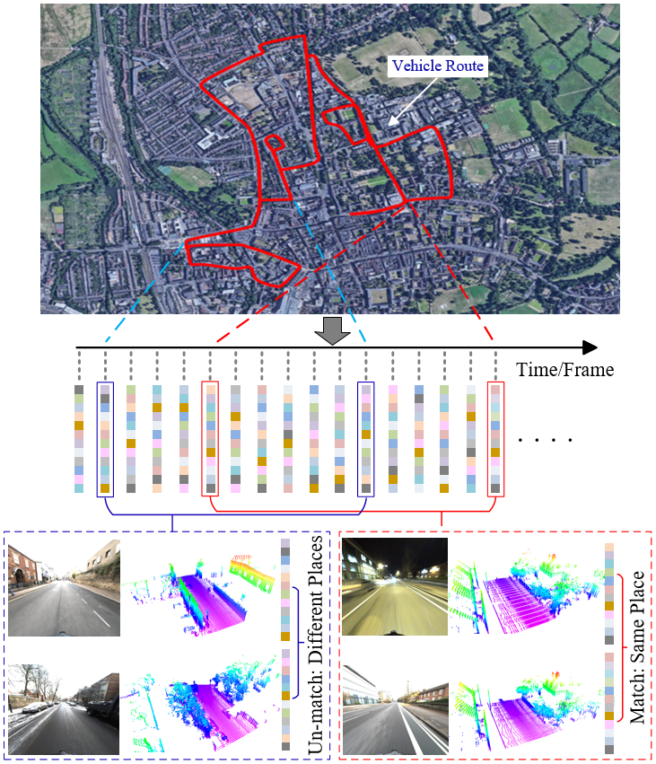
Figure 1: Place recognition in large-scale environments. We use global feature descriptors generated from the raw 3D point cloud data to accomplish place recognition tasks. The lower side shows two examples with different weather and light conditions.

Large-scale place recognition is of great importance in robotic applications, such as helping self-driving vehicles to obtain loop-closure candidates, achieve accurate localization and build drift-free globally consistent maps. Vision-based place recognition has been investigated for a long time and lots of successful solutions were presented. Thanks to the feasibility of extracting visual feature descriptors from a query image of a local scene, vision-based approaches have achieved good retrieval performance for place recognitions with respect to the reference map [19, 9]. However, vision-based solutions are not robust to season, illumination and viewpoint variations, and also suffer from performance degradations in the place recognition task with bad weather conditions. Taking into account the above limitations of the vision-based approach, 3D point cloud-based approach provides an alternative option, which is much more robust to season and illumination variations [22]. By directly using the 3D positions of each point as the network input, PointNet [11] provides a simple and efficient point cloud feature learning framework, but fails to capture fine-grained patterns of the point cloud due to the ignored point local structure information. Inspired by PointNet, different networks have been proposed [13, 23, 17, 5] and achieved advanced point cloud classification and segmentation results with the consideration of well-learned local features. However, it is hard to directly implement these networks to extract discriminative and generalizable global descriptors of the point cloud in large scenes. On the other hand, PointNetVLAD [22] is presented to solve the point cloud description problem in large-scale scenes, but it ignores the spatial distribution of similar local features, which is of great importance in extracting the static structure information in large-scale dynamic environments.

Attempting to address the above issues, we present LPD-Net to extracting discriminative and generalizable global features from large-scale point clouds. As depicted in Fig. 1, based on the generated global descriptor, we solve the point cloud retrieval task for large-scale place recognitions. Our contributions include: $1)$ We introduce local features in an adaptive manner as the network input instead of only considering the position of each isolated point, which helps to adequately learn the local structures of the input point cloud. $2)$ We propose a graph-based aggregation module in both Feature space and Cartesian space to further reveal the spatial distribution of local features and inductively learn the structure information of the whole point cloud. This contributes to learn a discriminative and generalizable global descriptors for large-scale environments. $3)$ We utilize the global descriptor for point cloud-based retrieval tasks to achieve large-scale place recognitions. Our LPD-Net outperforms PointNetVLAD in the point cloud based retrieval task and reaches the state-of-the-art. What’s more, compared with vision-based solutions, our LPD-Net shows comparable performance and is more robust to different weather and light conditions.

2 Related Work

Handcrafted local features, such as the histogram feature [14], the inner-distance-based descriptor [8] and the heat kernel signatures [21], are widely used for point cloud-based recognition tasks, but they are usually designed for specific applications and have a poor generalization ability. In order to solve these problems, deep learning based methods was presented for point cloud feature descriptions. Convolution neural network (CNN) has achieved amazing feature learning results for regular 2D image data. However, it is hard to extend the current CNN-based method to 3D point clouds due to their orderless. Some researches attempt to solve this problem by describing the raw point cloud by a regular 3D volume representation, such as the 3D ShapeNets [26], VoxNet [10], volumetric CNNs [12], VoxelNet [28] and 3D-GAN [25]. Some other methods, such as the DeepPano [18] and Multiview CNNs [20], project 3D point clouds into 2D images and use the 2D CNN to learn features. However, these approaches usually introduce quantization errors and high computational cost, hence hard to capture high-resolution features with high update rate.

PointNet [11] achieves the feature learning directly from the raw 3D point cloud data for the first time. As an enhanced version, PointNet++ [13] introduces the hierarchical feature learning to learn local features with increasing scales, but it still only operates each point independently during the learning process. Ignoring the relationship between local points leads to the limitation ability of revealing local structures of the input point cloud. To solve this, DG-CNN [23] and KC-Net [17] mine the neighborhood relations through the dynamic graph network and the kernel correlation respectively. Moreover, [5] captures local features by performing the kNN algorithm in the feature space and the k-means algorithm in the initial word space simultaneously. However, they obtain fine-grained features at the expense of ignoring the feature distribution information. What’s more, the performance of these approaches in large-scale place recognition tasks have not been validated.

Traditional point cloud-based large-scale place recognition algorithms [6] usually rely on a global, off-line, and high-resolution map, and can achieve centimeter-level localization, but at the cost of time-consuming off-line map registration and data storage requirements. SegMatch [4] presents a place matching method based on local segment descriptions, but they need to build a dense local map by accumulating a stream of original point clouds to solve the local sparsity problem. PointNetVLAD [22] achieves the state-of-the-art place recognition results. However, as mentioned before, it does not consider the local structure information and ignores the spatial distribution of local features. These factors, however, is proved in our ablation studies that will greatly improve the place recognition results.

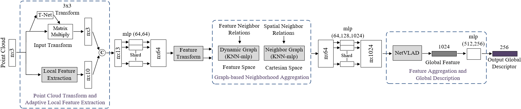
Figure 2: LPD-Net Architecture. The network takes the raw point cloud data as input, applies Adaptive Local Feature Extraction to obtain the point cloud distribution and the enhanced local features, which are aggregated both in the Feature Space and the Cartesian Space through the graph neural network. The resulted feature vectors are then utilized by NetVLAD [1] to generate a global descriptor.

3 Network Design

The objective of our LPD-Net is to extract discriminative and generalizable global descriptors from the raw 3D point cloud directly, and based on which, to solve the point cloud retrieval problems. Using the extracted global descriptor, the computational and storage complexity will be greatly reduced, thus enabling the real-time place recognition tasks. We believe that the obtained place recognition results will greatly facilitate the loop closure detection, localization and mapping tasks in robotics and self-driving applications.

3.1 The Network Architecture

As we mentioned above, most of the existing work is done on the small-scale object point cloud data (e.g. ModelNet [26] and ShapeNet [27]), but this is not the case for large-scale environments, since such point clouds are mainly composed of different objects in the scene and with unknown relationships between the objects. In contrast, we have customized for large-scale environments and proposed a network with three main modules, $1)$ Feature Network (FN), $2)$ Graph-based Neighborhood Aggregation, and $3)$ NetVLAD [1]. The complete network architecture of LPD-Net is shown in Fig. 2. The NetVLAD is designed to aggregate local feature descriptors and generate the global descriptor vector for the input data. Similar to [22], the loss function of the network uses lazy quadruplet loss based on metric learning, so that the positive sample distance is reduced during the training process and the negative sample distance is enlarged to obtain a unique scene description vector. In addition, it has been proven to be permutation invariant, thus suitable for 3D point cloud.

3.2 Feature Network

Existing networks [11, 13, 22] only use the point position as the network input, local structures and point distributions have not been considered. This limits the feature learning ability [7]. Local features usually represent the generalized information in the local neighborhood of each point, and it has been successfully applied to different scene interpretation applications [24, 4]. Inspired by this, our FN introduces local features to capture the local structure around each point.

3.2.1 Feature Network Structure

The raw point cloud data is simultaneously input to the Input Transformation Net [11] and the Adaptive Local Feature Extractor (as will be introduced in Section 3.2.2), the former aims to ensure the rotational translation invariance [11] of the input point coordinates, and the latter aims to fully consider the statistical local distribution characteristics. It should be noted that, the point cloud acquired in large-scale scenes often has uneven local point distributions, which may affect the network accuracy. To handle this, the adaptive neighborhood structure is considered to select the appropriate neighborhood size according to different situations to fuse the neighborhood information of each point. We then map the above two kinds of features (with the concatenation operation) to the high-dimensional space, and finally make the output of FN invariant to the spatial transformation through the Feature Transformation Net.

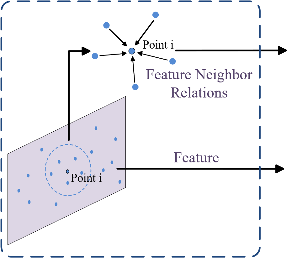
(a) FN-Original structure (O)

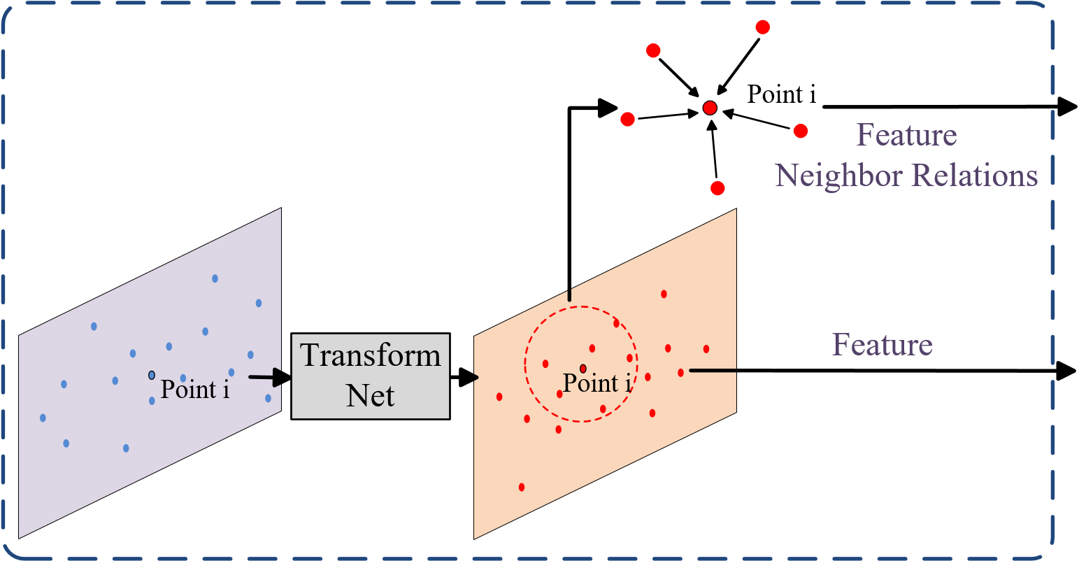
(b) FN-Series structure (S)

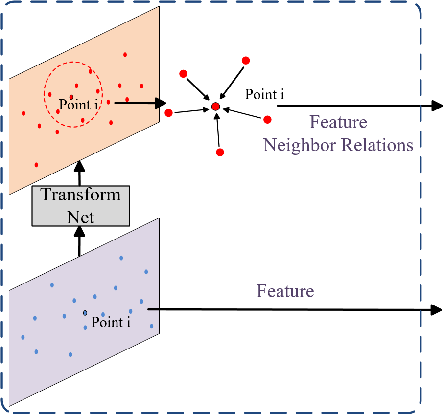
(c) FN-Parallel structure (P)

Figure 3: Different network structures for feature transformation and relation extraction.

3.2.2 Adaptive Local Feature Extraction

We introduce local distribution features by considering the local 3D structure around each point $i$. $k$ nearest neighboring points are counted and the respective local 3D position covariance matrix is considered as the local structure tensor. Without loss of generality, we assume that $\lambda^{i}_{1}\geq\lambda^{i}_{2}\geq\lambda^{i}_{3}\geq 0$ represent the eigenvalues of the symmetric positive-define covariance matrix. According to [24], the following measurement can be used to describe the unpredictability of the local structure from the aspect of the Shannon information entropy theory,

$$E_{i}=-L_{i}\ln{L_{i}}-P_{i}\ln{P_{i}}-S_{i}\ln{S_{i}},$$ (1)

where $L_{i}=\frac{\lambda^{i}_{1}-\lambda^{i}_{2}}{\lambda^{i}_{1}}$, $P_{i}=\frac{\lambda^{i}_{2}-\lambda^{i}_{3}}{\lambda^{i}_{1}}$ and $S_{i}=\frac{\lambda^{i}_{3}}{\lambda^{i}_{1}}$ represent the linearity, planarity and scattering features of the local neighborhood of each point respectively. These features describe the 1D, 2D and 3D local structures around each point [24]. Since the point distribution in a point cloud is typically uniform, we adaptively choose the neighborhood of each point $i$ by minimizing $E_{i}$ across different $k$ values and the optimal neighbor size is determined as

$$k^{i}_{opt}=\arg\min_{k}E_{i}(k).$$ (2)

Local features suitable for describing large-scale scenes can be classified into four classes: eigenvalue-based 3D features ($F_{3D}$), features arising from the projection of the 3D point onto the horizontal plane ($F_{2D}$), normal vector-based features ($F_{V}$), and features based on Z-axis statistics ($F_{Z}$). Existing researches have validated that $F_{3D}$, $F_{V}$ and $F_{Z}$ are effective in solving the large-scale 3D scene analysis problem [24], and $F_{2D}$ and $F_{Z}$ are effective in solving the large-scale localization problem in self-driving tasks[3, 4]. Considering the feature redundancy and discriminability, we select the following ten local features to describe the local distribution and structure information around each point $i$:

• $F_{3D}$ features: Change of curvature $C_{i}=\frac{\lambda^{i}_{3}}{\sum_{j=1}^{3}\lambda^{i}_{j}}$, Omni-variance $O_{i}=\frac{\sqrt[3]{\prod_{j=1}^{3}\lambda^{i}_{j}}}{\sum_{j=1}^{3}\lambda^{i}_{j}}$, Linearity $L_{i}=\frac{\lambda^{i}_{1}-\lambda^{i}_{2}}{\lambda^{i}_{1}}$, Eigenvalue-entropy $A_{i}=-\sum_{j=1}^{3}(\lambda^{i}_{j}\ln\lambda^{i}_{j})$, and Local point density $D_{i}=\frac{k^{i}_{opt}}{\frac{4}{3}\prod_{j=1}^{3}\lambda^{i}_{j}}$.

• $F_{2D}$ features: 2D scattering $S_{i,2D}=\lambda^{i}_{2D,1}+\lambda^{i}_{2D,2}$ and 2D linearity $L_{i,2D}=\frac{\lambda^{i}_{2D,2}}{\lambda^{i}_{2D,1}}$, where $\lambda^{i}_{2D,1}$ and $\lambda^{i}_{2D,2}$ represent the eigenvalues of the corresponding 2D covariance matrix.

• $F_{V}$ feature: Vertical component of normal vector $V_{i}$.

• $F_{Z}$ features: Maximum height difference $\Delta Z_{i,\max}$ and Height variance $\sigma Z_{i,var}$.

3.2.3 Feature Transformation and Relation Extraction

In the output of the Adaptive Local Feature Extraction module, each data can be regarded as the feature description of the surrounding neighborhood since we have merged the neighborhood structure into the feature vector of the neighborhood center point. Three structures are then designed in the Feature Transform module shown in Fig. 2 to further reveal the relations between the local features:

• FN-Original structure (Fig. 3(a)): The two outputs are the feature vector $f_{F}$ and the neighborhood relation vector $f_{R}$ by performing kNN operations on $f_{F}$.

• FN-Series structure (Fig. 3(b)): The two outputs are the feature vector $f_{FT}$ which has been transformed by the Transform Net [11], and the neighborhood relation vector $f_{RT}$ by performing kNN operations on $f_{FT}$.

• FN-Parallel structure (Fig. 3(c)): The two outputs are the feature vector $f_{F}$ and the neighborhood relation vector $f_{RT}$, where $f_{RT}$ is the same with that in FN-Series structure.

The ablation study in Section 4.2 reveals that the FN-Parallel structure is the best one in our case.

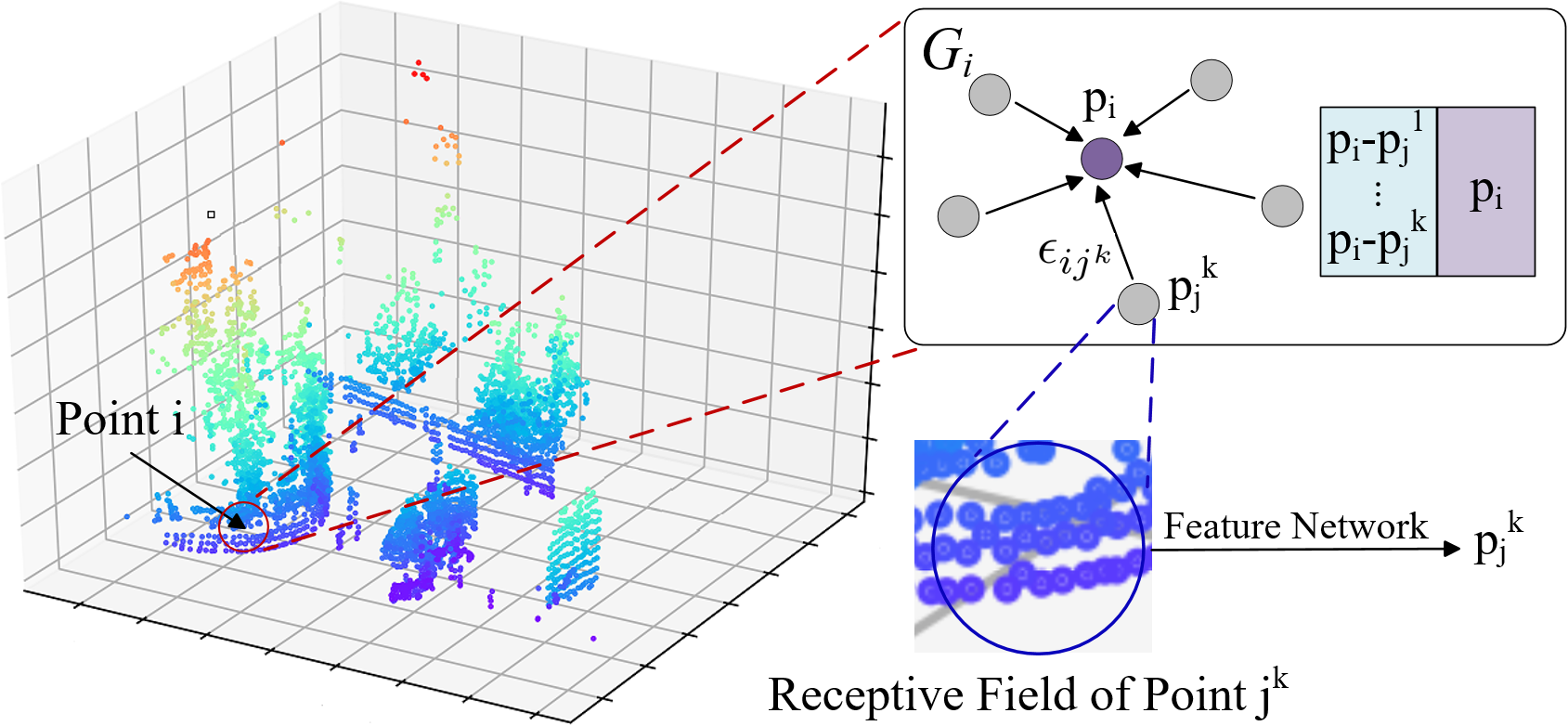
Figure 4: Graph formulation. Note that the receptive field of each point corresponds to a local neighborhood in the original point cloud, since the FN has introduced the local structure into the feature of each point. Then we utilize GNN for feature aggregations.

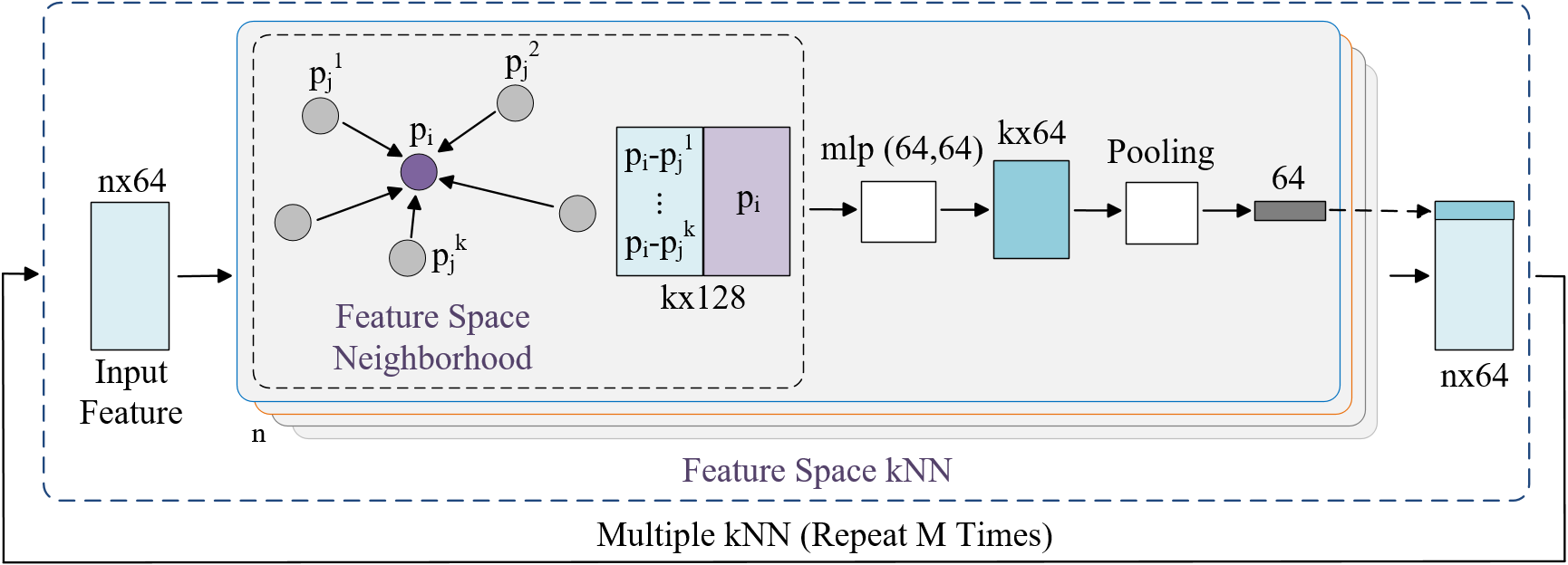
Figure 5: Feature space graph-based neighborhood aggregation.

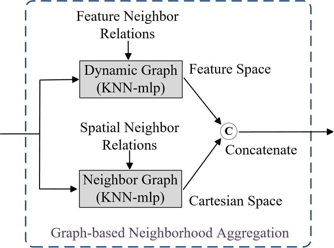
(a) Prarllel-Concatenation structure (PC)

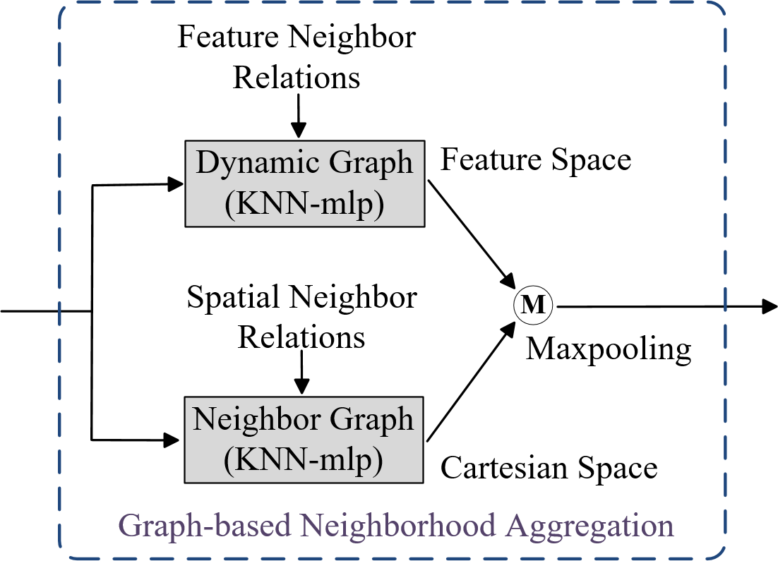
(b) Parallel-Maxpooling structure (PM)

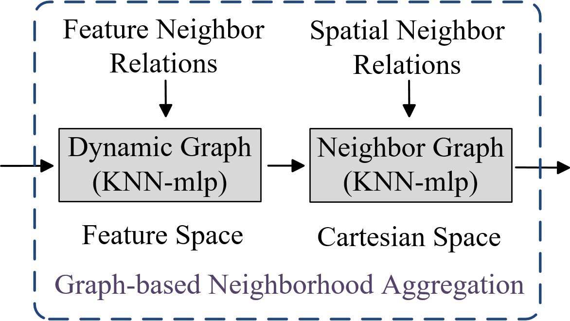
(c) Series-FC structure (SF)

Figure 6: Different network structures for feature aggregation.

3.3 Graph-based Neighborhood Aggregation

Different with the object point clouds, the point clouds of large-scale environments mostly contain several local 3D structures (such as planes, corners, shapes, etc.) of surrounding objects. Similar local 3D structures which locate in different parts of the point cloud usually have similar local features. Their spatial distribution relationships are also of great importance in place description and recognition tasks. We introduce the relational representation from the Graph Neural Network (GNN) [2] into our LPD-Net, which uses a structured representation to get the compositions and their relationship. Specifically, we represent the compositions of the scene as the nodes in the graph model (Fig. 4), and represent their intrinsic relationships and generate unique scene descriptors through GNN.

3.3.1 Graph Neural Network Structure

The outputs of the Feature Network (the feature vector and the neighborhood relation vector) are used as the input of the graph network, and feature aggregation is performed in both the feature space and the Cartesian space. As shown in Fig. 5, in the feature space, we build a dynamic graph $G_{i,d}$ for each point $i$ through the multiple kNN iterations. More specifically, in each iteration, the output feature vector of the previous iteration is used as the network input and a kNN aggregation is conducted on each point by finding $k$ neighbors with the nearest feature space distances. This is similar to CNN to achieve the multi-scale feature learning. Each point feature $p_{i}$ is treated as a node in the graph. Each edge $\epsilon_{ij}^{m}$ represents the feature space relation between $p_{i}$ and its $k$ nearest neighbors $p_{j}^{m}$ in the feature space, and $\epsilon_{ij}^{m}$ is defined as $\epsilon_{ij}^{m}=p_{i}-p_{j}^{m},m={1,2,...,k}$. The mlp network is used to update neighbor relations and the max pooling operation is used to aggregate $k$ edge information into a feature vector to update the point feature $p_{i}$. Note that the features of two points with a large Cartesian space distance can also be aggregated for capturing similar semantic information, due to the graph-based feature learning in the feature space. In addition, the neighborhood information in the Cartesian space should also be concerned. The kNN-graph network is also implemented in the Cartesian space. The node and edge are defined as the same in the feature space and the only difference is that we consider the Euclidean distance to build the kNN relations.

3.3.2 Feature Aggregation Structure

In LPD-Net, GNN modules in the feature space and the Cartesian space aggregate neighborhood features and spatial distribution information separately. We designed three different structures to further aggregate these two modules:

• Prarllel-Concatenation structure (PC, Fig. 6(a)): Cascade the output feature vectors of the two modules and merge the dual-dimensional information through MLP to aggregate the features.

• Parallel-Maxpooling structure (PM, Fig. 6(b)): Directly integrate the output feature vectors of the two models through the max pooling layer, taking the maximum values to generate the unified feature vector.

• Series-FC structure (SF, Fig. 6(c)): The output feature vector of one module is utilized as the input feature of the other module.

The experimental result in Section 4.1 reveals that the SF structure with the order shown in Fig. 6(c) is the best one in our case.

3.4 Discussion

Based on the proposed LPD-Net, we can analyze the environment by studying the statistical characteristics of all the global descriptors, such as calculating the similarity of two places by the $L_{2}$ distance between the two corresponding global descriptors, or evaluating the uniqueness of each place by calculating its distance to all the other places. More details can be found in our supplementary materials.

4 Experiments

Table 1: LDP-Net configuration.

NN-VLAD

FN-VLAD

FN-NG-VLAD

FN-DG-VLAD

FN-PM-VLAD

FN-PC-VLAD

FN-SF-VLAD

point-3

mlp-10

point-3

ALF-10

point-3

ALF-10

point-3

ALF-10

point-3

ALF-10

point-3

ALF-10

point-3

ALF-10

T-Net-3

T-Net-3

T-Net-3

T-Net-3

T-Net-3

T-Net-3

T-Net-3

concat-13

concat-13

concat-13

concat-13

concat-13

concat-13

concat-13

mlp-64

mlp-64

mlp-64

mlp-64

mlp-64

mlp-64

mlp-64

mlp-64

mlp-64

mlp-64

mlp-64

mlp-64

mlp-64

mlp-64

Feature transform-64 and relation extraction-feature space KNN (Kf) & Cartesian space KNN (Kc)

KNN-Kc*64

KNN-Kf*64

KNN-Kf*64

KNN-Kc*64

KNN-Kf*64

KNN-Kc*64

KNN-Kf*64

mlp-64

EF-k*128

EF-k*128

mlp-64

EF-k*128

mlp-64

EF-k*128

mlp-64

mlp-64

mlp-64

mlp-64

mlp-64

mlp-64

mlp-64

mlp-64

mlp-64

mlp-64

mlp-64

maxpooling-64

maxpooling-64

maxpooling-64

concat-64

maxpooling-64

KNN-Kc*64

mlp-64

mlp-64

maxpooling-64

FC-64

FC-128

FC-1024

L2-normalization

NetVLAD-D

L2-normalization

Lazy Quadruplet Loss

• ALF: Adaptive local feature.

The configuration of LPD-Net is shown in Tab. 1. In NetVLAD [1, 22], the lazy quadruplet loss paremeters are set as $\alpha=0.5,\beta=0.2,P_{pos}=2,P_{neg}=18$. We train and evaluate the network on the modified Oxford Robotcar dataset presented by [22], which includes 44 data sets from the original Robotcar dataset, with 21,711 training submaps and 3030 testing submaps. We also directly transplant the trained model to the In-house Dataset [22] for evaluation and verify its generalization ability. Please not that in all datasets, the point data has been randomly down-sampled to 4096 points and normalized to [-1,1]. More details of the datasets can be found in [22]. All experiments are conducted with a 1080Ti GPU on TensorFlow.

4.1 Place Recognition Results

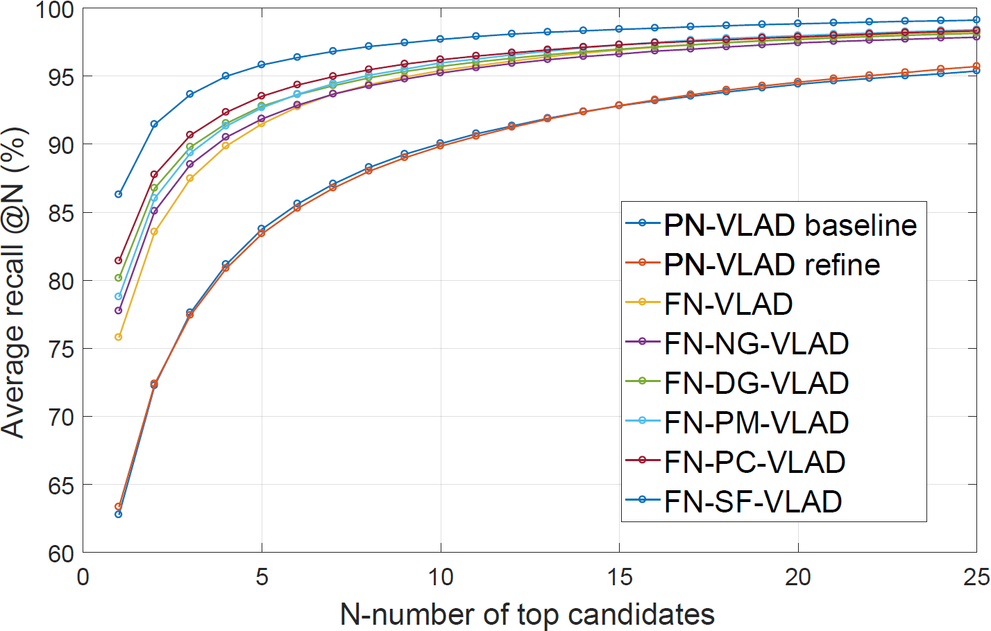
Figure 7: Average recall under different networks.

Table 2: Comparison results of the average recall (%) at top 1% (@1%) and at top 1 (@1) under different networks.

	Ave recall @1%	Ave recall @1
PN STD	$46.52$	$31.87$
PN MAX	$73.87$	$54.16$
PN-VLAD baseline∗	$81.01$	$62.76$
PN-VLAD refine∗	$80.71$	$63.33$
NN-VLAD (our)	$79.21$	$61.96$
FN-VLAD (our)	$89.77$	$75.79$
FN-NG-VLAD (our)	$90.38$	$77.74$
FN-DG-VLAD (our)	$91.44$	$80.14$
FN-PM-VLAD (our)	$91.20$	$78.77$
FN-PC-VLAD (our)	$92.27$	$81.41$
FN-SF-VLAD (our)	$\bf{94.92}$	$\bf{86.28}$

• ^∗This result is obtained by using their open-source programs.

Table 3: Comparison results of the memory and computation required under different networks.

	Parameters	FLOPs	Runtime per frame
PN-VLAD baseline	1.978M	411M	13.09ms
FN-PM-VLAD (our)	1.981M	749M	29.23ms
FN-PC-VLAD (our)	1.981M	753M	27.03ms
FN-SF-VLAD (our)	1.981M	749M	23.58ms

• FLOPs: required floting-point operations.

The selected Robotcar dataset contains the point clouds collected in various season and weather conditions and different times. We query the same scene in these different sets for place recognition tasks. Specifically, we use the LPD-Net to generate the global descriptors and query the scene with the closest $L_{2}$ distance (in the descriptor space) to the test scene to determine whether it is the same place. Similar to [22], the Recall indices, including the Average Recall@N and Average Recall@1%, are utilized to evaluate the place recognition accuracy. We compare our LPD-Net with the original PointNet architecture with the maxpool layer (PN MAX) and the PointNet trained for object classification in ModelNet (PN STD) to see whether the model trained on small-scale object datesets can be scaled to large-scale cases. We also compare our LPD-Net with the state-of-the-art PN-VLAD baseline and PN-VLAD refine [22]. We evaluate the PN STD, PN MAX, PN-VLAD baseline and PN-VLAD refine on the Oxford training dataset. The network configurations of PN STD, PN MAX, PN-VLAD baseline and refine are set to be the same as [11, 22].

Comparison results are shown in Fig. 7 and Tab. 2, where FN-PM-VLAD, FN-PC-VLAD, and FN-SF-VLAD represent our network with the three different feature aggregation structures PM, PC, and SF. FN-VLAD is our network without the graph-based neighborhood aggregation module. DG and NG represent the Dynamic Graph and Neighbor Graph in the proposed graph-based neighborhood aggregation module. Additionally, we also design the NeuralNeighborVLAD network (NN-VLAD), which uses kNN clustering (k=20) and mlp module to replace the adaptive local feature extraction module presented in Section 3.2.2. The output of the network is also a 10 dimensional neighborhood feature, and the features are obtained through network learning. Thanks to the adaptive local feature extraction and graph neural network modules, our LPD-Net has superior advantages for place recognition in large-scale environments. What’s more, among the three aggregation structures, FN-SF-VLAD is the best one, far exceeding PointNetVLAD from $81.01\%$ to $94.92\%$ at top 1% (unless otherwise stated, the LPD-Net represents the FN-SF-VLAD in this paper). In SF, the graph neural network learns the neighborhood structure features of the same semantic information in the feature space, and then further aggregates them in the Cartesian space. So we believe that SF can learn the spatial distribution characteristics of neighborhood features, which is of great importance for large-scale place recognitions. In addition, PC is better than PM since it reserves more information. The computation and memory required for our networks and the PN-VLAD baseline are shown in Tab. 3. For our best results (FN-SF-VLAD), We have a 13.81% increase in retrieval results (at top 1%) at the cost of an average of 10.49ms added to per frame.

Table 4: Indoor datasets evaluation results (Ave recall @ 1%).

	U.S.	R.A.	B.D.
PN-VLAD baseline	72.63	60.27	65.30
PN-VLAD refine	90.10	93.07	86.49
FN-SF-VLAD (our)	96.00	90.46	89.14

Similar to [22], we also test our network in the Indoor Dataset [22], as shown in Tab.4. Please note that we only train our netowrk on the Oxford Robotcar dataset and directly test it on the three indoor datasets, however, PointNetVLAD-refine results are obtained by training the network both on the Oxford dataset and the indoor datasets.

4.2 Ablation Studies

Different Local Features: We test our LPD-Net with different local features, where $xyz-$ represent the coordinates of each point, $F_{2D}$ and $F_{3D}$ are defined in Section 3.2.2, $FN$ represents the feature network with the proposed ten local features. In $full$, we add four $F_{3D}$ features (Planarity, Scattering, Anisotropy and Sum of eigenvalues [24]) in addition to the proposed ten local features, namely, a total of 14 local features are considered. Tab. 5 shows that $F_{2D}$ features have larger contributions than $F_{3D}$ features, and additional features do not contribute to improve the network accuracy since some of the features are linearly related.

Table 5: Ablation studies of different local features.

	Ave recall @1%	Ave recall @1
xyz-SF-VLAD	$84.74$	$69.75$
FN(non-$F_{2D}$)-SF-VLAD	$90.76$	$76.94$
FN(non-$F_{3D}$)-SF-VLAD	$91.23$	$79.11$
FN-SF-VLAD	$\bf{94.92}$	$\bf{86.28}$
FN(full)-SF-VLAD	$92.03$	$81.45$

Table 6: Ablation studies of different feature neighbor relations.

	Ave recall @1%	Ave recall @1
xyz-Series-VLAD	$83.22$	$66.01$
xyz-Parallel-VLAD	$84.74$	$69.75$
FN-Original-VLAD (O)	$91.53$	$80.29$
FN-Series-VLAD (S)	$92.60$	$81.09$
FN-Parallel-VLAD (P)	$\bf{94.92}$	$\bf{86.28}$

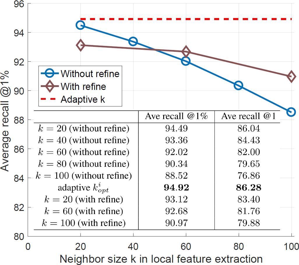
Figure 8: Ablation studies of different neighbor size $k$ in the local feature extraction.

Table 7: Ablation studies of different feature dimension $D$ and the number of visual words $K$ in NetVLAD.

	Ave recall @1%	Ave recall @1
$D_{256}K_{32}$	$93.91$	$85.02$
$D_{256}K_{64}$	$\bf{94.92}$	$\bf{86.28}$
$D_{256}K_{128}$	$92.47$	$82.08$
$D_{512}K_{32}$	$92.92$	$83.01$
$D_{512}K_{64}$	$94.66$	$85.80$
$D_{512}K_{128}$	$93.58$	$84.25$

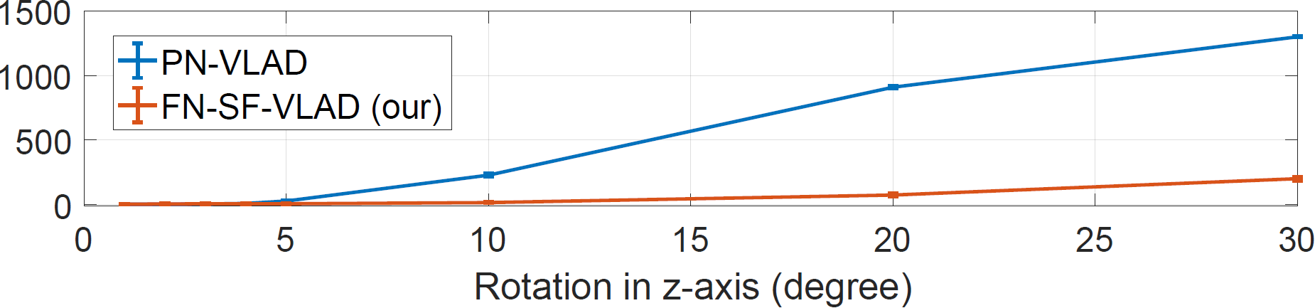
Figure 9: The number of place recognition mistakes in the robustness test.

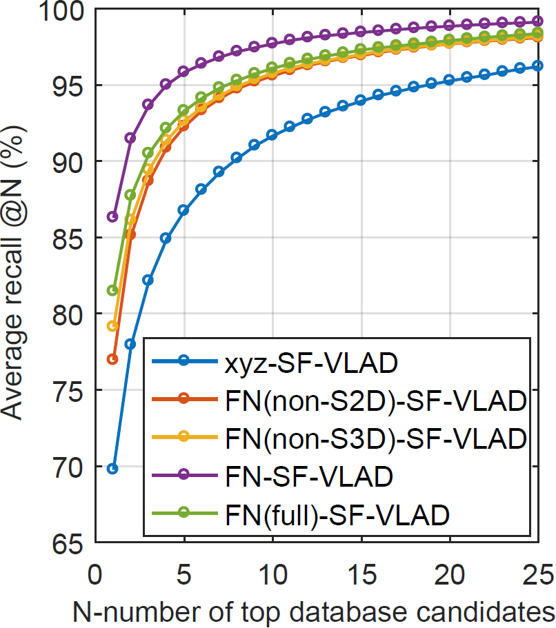
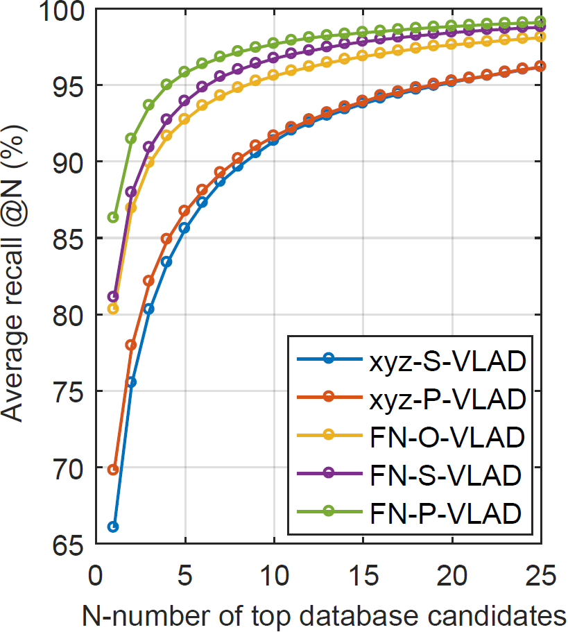
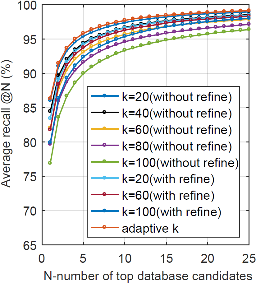
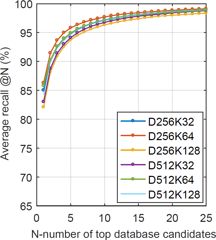
Figure 10: Ablation study results: (a).Different local features. (b).Different feature neighbor relations. (c).Different neighbor size $k$ in the local feature extraction.(d).Different feature dimension $D$ and the number of visual words $K$ in NetVLAD.

Table 8: Comparisons with vision-based methods (Ave recall @1 with different GPS location bounds: 3m/5m/10m/15m).

	dawn	dusk	overcast$\_$summer	overcast$\_$winter	night-rain	sun	night
Our LPD-Net	65.1$/$79.7$/$86.5$/$88.4	64.7$/$79.9$/$87.3$/$89.8	63.5$/$79.7$/$85.3$/$86.8	45.6$/$73.8$/$79.2$/$81.0	20.1$/$32.8$/$40.6$/$44.6	74.1$/$82.3$/$87.8$/$89.4	63.2$/$77.3$/$83.1$/$84.5
HF-Net [15]	45.3$/$71.2$/$81.0$/$84.7	54.1$/$85.8$/$92.6$/$93.9	55.5$/$78.8$/$83.2$/$84.7	31.3$/$75.4$/$86.9$/$89.5	2.7$/$6.6$/$10.5$/$11.4	54.6$/$68.3$/$75.7$/$81.7	2.1$/$3.9$/$7.1$/$7.3
NV [1]	50.9$/$80.1$/$85.5$/$88.4	54.1$/$88.6$/$96.2$/$97.7	68.9$/$92.2$/$95.2$/$96.8	29.7$/$81.0$/$94.9$/$96.7	5.7$/$14.3$/$19.5$/$22.3	70.0$/$82.4$/$87.6$/$89.3	9.4$/$17.1$/$23.7$/$26.9
NV+SP [15]	43.7$/$67.7$/$82.2$/$88.6	45.0$/$63.4$/$86.5$/$92.6	48.8$/$68.7$/$84.9$/$92.7	27.2$/$60.0$/$86.7$/$93.8	9.3$/$18.6$/$25.0$/$28.4	48.0$/$64.3$/$84.8$/$92.4	11.2$/$19.2$/$29.0$/$33.6

Different Feature Neighbor Relations: We test our LPD-Net with different feature neighbor relations shown in Fig. 3. Tab. 6 shows that $P$ is better than $O$ and $S$, which implies that only utilizing the feature relations in the transformed feature space and remaining the original feature vectors can achieve the best result. Please note that in PointNet and PointNetVLAD, they use the $S$ relation.

Different Neighbor Size $k$ in the Local Feature Extraction: Fig. 8 shows that, in the case of constant $k$, the accuracy decreases with the size of $k$. With refinements (retrain the network with the fixed $k$), the accuracy is still lower than that of the proposed adaptive approach ($k_{opt}^{i}$).

Different $K$ and $D$ in NetVLAD: NetVLAD has two unique hyper-parameters: the feature dimension $D$ and the number of visual words $K$ [1, 22]. Tab. 7 shows that the values of $K$ and $D$ should be matched in order to achieve a good accuracy. We use $K=64$ and $D=256$ in this paper.

All the above ablation studies are conducted on the robotcar dataset. The detailed results are shown in Fig. 10.

Robustness Test: We rotate the input point cloud and add $10\%$ random white noise to validate the robustness of our LPD-Net. The results are shown in Fig. 9, more details can be found in our supplementary materials.

4.3 Comparison with image-based methods

To further investigate the advantages of our LPD-Net, the preliminary comparison results with the state-of-the-art image-based solutions are shown in Tab. 8, where NV is a pure NetVLAD method, HF-Net and NV+SP are proposed in [15]. This comparison is conducted on the Robotcar Seasons dataset [16], and we generate the corresponding point clouds by using the original data from the Robotcar dataset. We can observe that, in the most of the cases, our point cloud-based method shows strong performance on par or even better than image-based methods. A special case lies in the night-rain scene, since the point cloud data used here is reconstructed using a single-line LiDAR and visual odometry (VO), the inaccuracy of VO causes the point cloud to be distorted, hence resulting in a reduced result. However, we can still observe that our method significantly outperforms other approachs in the night-rain case. Fig. 11 shows three examples in different cases. In these examples, the image-based solution obtains the unsuccessfully retrieved images, due to the bad weather and light conditions. However, our LPD-Net obtains the correct results.

Please noted that the presented work at this stage only focuses on the point cloud-based place recognition, however, the above image-based solutions are proposed for the pose estimation task, so the above comparisons are not rigorous. In the future, we will improve our LPD-Net in order to solve the pose estimation problem.

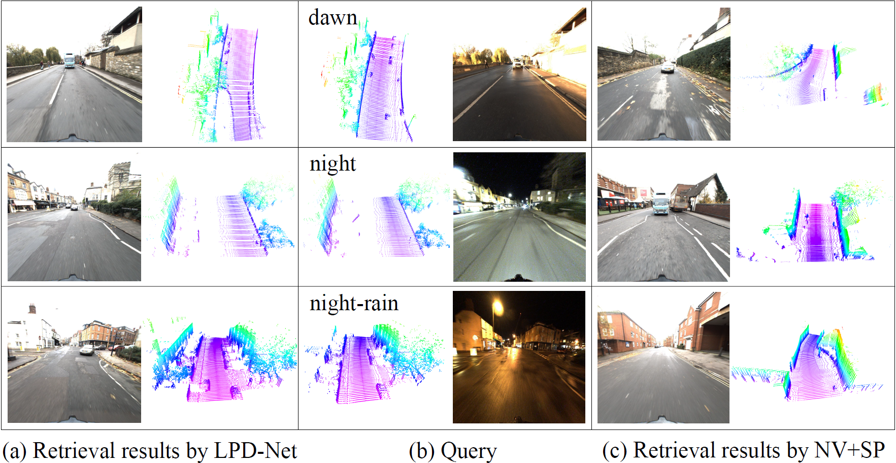
Figure 11: Examples of the retrieval results of our LPD-Net and the image-based solution NV+SP [15]. The middle column shows the query images and point clouds, the left column shows the retrieved point clouds by LPD-Net and their corresponding images, the right column shows the retrieved images by NV+SP and their corresponding point clouds.

5 Conclusion

In this paper, we present the LPD-Net that solves the large-scale point cloud-based retrieval problem so that the reliable place recognition can be successfully performed. Experimental results on benchmark datasets validate that our LPD-Net is much better than PointNetVLAD and reaches the state-of-the-art. What’s more, comparison results with image-based solutions validate the robustness of our LPD-Net under different weather and light conditions.

6 Supplementary Material

6.1 Detailed differences between our network and existing networks

Comparison of the proposed network with existing methods is shown in Table 9. PointNet [11] provides a simple and efficient point cloud feature learning framework that directly uses the raw point cloud data as the input of the network, but failed to capture fine-grained patterns of the point cloud due to the ignored local features of points. PointNet++ [13] considers the hierarchical feature learning, but it still only operates each point independently during the local feature learning process, which ignores the relationship between points, leading to the missing of local feature. Then, KCNet [17] and DGCNN [23] have been designed based on PointNet. With the kNN-based local feature aggregating in the feature space, the state-of-the-art classification and segmentation results are obtained on small-scale object point cloud dataset. Moreover, RWTH-Net [5] achieved fine-grained segmentation results on the large-scale outdoor dataset based on local feature aggregating and clustering in Feature space and Cartesian space, respectively. However, the above networks all focus on capturing the similarity of point clouds, and it is hard to generate effective global descriptors of the point cloud in large scenes. On the other hand, PointNetVLAD [22] can learn the global descriptor of the point cloud in a large scene, but it only performs feature aggregation in the feature space, ignoring the distribution of features in Cartesian space, which makes it difficult to generalize the learned features.

Table 9: Where our work fits into the literature.

	Local features	Feature space aggregation	Cartesian space aggregation	Feature distribution	Large-scale scene
PointNet [11]
PointNet++ [13]			$\checkmark$
PointNetVLAD [22]		$\checkmark$			$\checkmark$
DGCNN [23]		$\checkmark$
KCNet [17]		$\checkmark$
RWTH-Net [5]		$\checkmark$	$\checkmark$		$\checkmark$
Our LPD-Net	$\checkmark$	$\checkmark$	$\checkmark$	$\checkmark$	$\checkmark$

6.2 Detailed environment analysis results

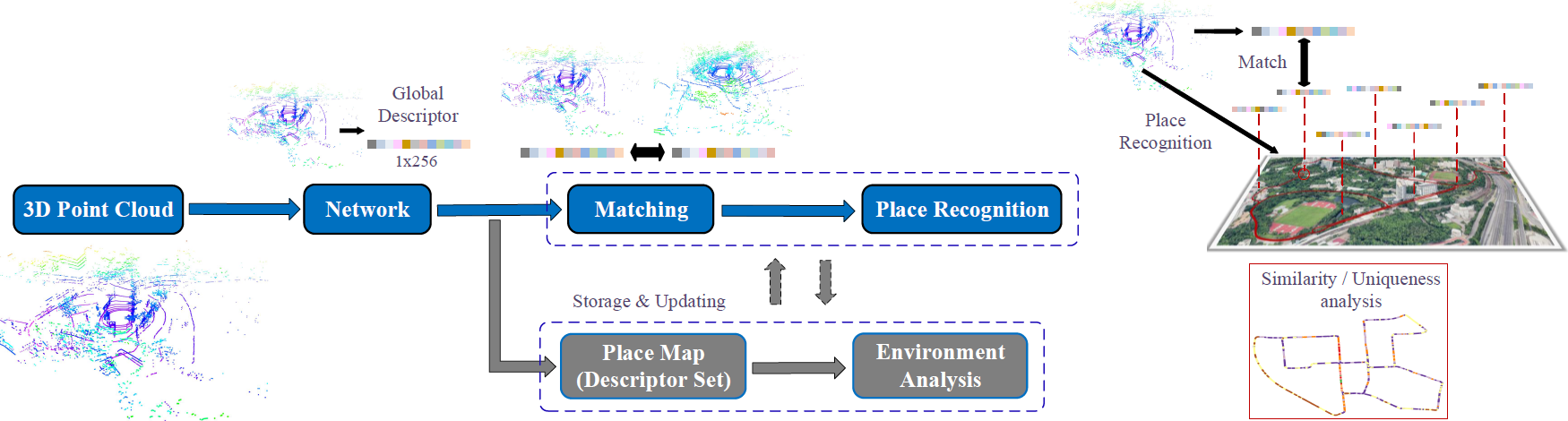
Figure 12: System structure.

Our LPD-Net extracts discriminative and generalizable global descriptors of an input point cloud, so we can resolve the large-scale place recognition and environment analysis problems. The system structure is shown in Fig. 12. The original 3D Lidar point cloud is used as system input directly. We use LPD-Net to extract a global descriptor which will be stored in a descriptor set. On the one hand, when a new input point cloud is obtained, we match its descriptor with those in the descriptor set to detect that whether the new scene corresponds to a previously visited place, if so, a loop closure detection accomplished. On the other hand, we analyze the environment by investigating the statistical characteristics of the global descriptors of the already visited places to evaluate the similarity/uniqueness of each place. The similarity between two point clouds is calculated from the distance between two corresponding global descriptors. Then for a given point cloud, we can calculate the similarity index of this point and plot a similarity map as shown in Fig. 13 (in KITTI dataset). With normalization, the sum of the similarity with all the other point clouds in the whole environment can be used to evaluate the uniqueness of the given point cloud (the given place). Fig. 14 shows the uniqueness evaluation results of the whole environment in KITTI dataset.

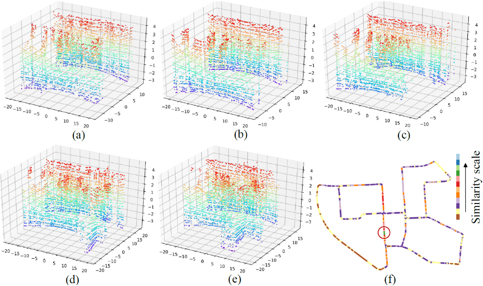
Figure 13: Similarity evaluation. (a)-(e) show a sequence of point clouds with near locations (correspond to the places within the red circle in f). (f) shows the similarity between the point cloud in (b) and all the other point clouds in the whole environment.

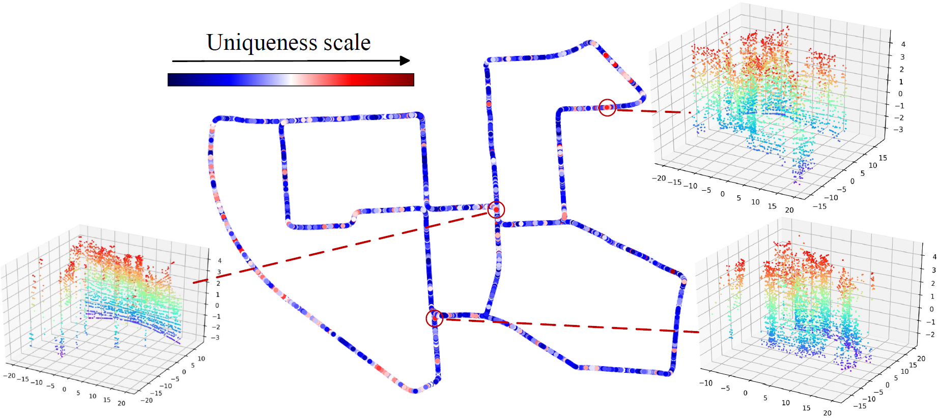
Figure 14: Uniqueness evaluation. The corresponding point clouds of three places with high uniqueness are shown.

We also cluster the global descriptors generated by our LPD-Net to see the places in the same cluster. We collect the point cloud data with a VLP-16 LADAR in our university campus. In Fig. 16, we show the clustered places which are also near with each other in the geographical location, and in Fig. 17, we show the clustered places which are far from each other in the geographical location.

6.3 Detailed robustness test results

The detailed results of the robustness test presented in the main paper are shown in Tab. 10 and Fig. 15. In Tab. 10, we show the average (max) number of place recognition mistakes under different degrees of input point cloud rotations. We consider 1580 places in the university campus dataset and also add 10% white noise in the tests. Both results from our network and PointNetVLAD are shown. Fig. 15 shows an example of the failure cases in PointNetVLAD in the robustness tests.

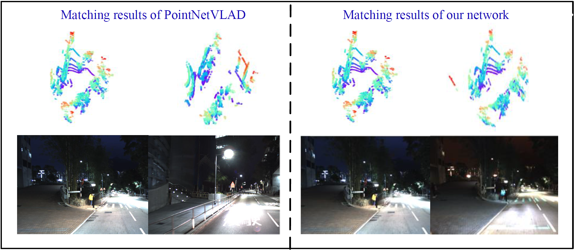
Figure 15: An Example of the failure cases in PointNetVLAD in the robustness tests. In this case, we rotate the input point cloud with 10 degrees and add 10% random white noise. Our network recognizes the place correctly, however, PointNetVLAD retrieves a wrong place.

Table 10: Results in the robustness test: with different rotation angles (degree).

	1	2	3	4	5	10	20	30
PointNetVLAD	4.5(6)	5.25(7)	7.75(13)	10.75(12)	29.25(31)	229.25(232)	908.75(918)	1298.75(1301)
Our LPD-Net	4.75(6)	6(8)	6.5(8)	7.25(9)	8(10)	17.25(21)	75.5(87)	202(217)

• A(B): A is the average number across eight repeated experiments in each case, B is the max number in the eight experiments.

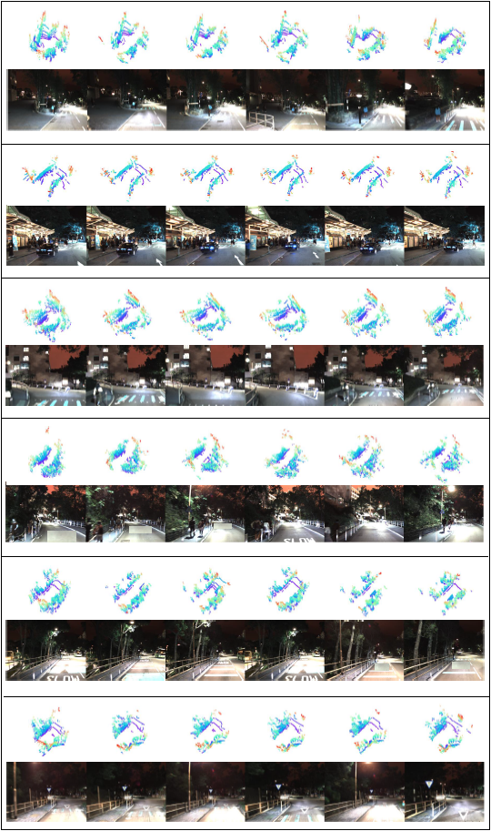
Figure 16: Examples of the place clustering results: the clustered places which are also near with each other in the geographical location.

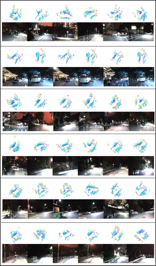
Figure 17: Examples of the place clustering results: the clustered places which are far from each other in the geographical location.

References

- [1] Relja Arandjelović, Petr Gronat, Akihiko Torii, Tomas Pajdla, and Josef Sivic. Netvlad: Cnn architecture for weakly supervised place recognition. In Proceedings of the IEEE Conference on Computer Vision and Pattern Recognition, pages 5297–5307, 2016.
- [2] Peter W. Battaglia, Jessica B. Hamrick, and Victor Bapst. Relational inductive biases, deep learning, and graph networks. In arXiv:1806.01261v2, 2018.
- [3] Xiaozhi Chen, Huimin Ma, Ji Wan, Bo Li, and Tian Xia. Multi-view 3d object detection network for autonomous driving. In Proceedings of the IEEE Conference on Computer Vision and Pattern Recognition, pages 6526–6534, 2017.
- [4] Renaud Dubé, Daniel Dugas, Elena Stumm, Juan Nieto, Roland Siegwart, and Cesar Cadena. Segmatch: Segment based place recognition in 3d point clouds. In Proceedings of the IEEE International Conference on Robotics and Automation, pages 5266–5272, 2017.
- [5] Francis Engelmann, Theodora Kontogianni, Jonas Schult, and Bastian Leibe. Know what your neighbors do: 3d semantic segmentation of point clouds. In Proceedings of the IEEE European Conference on Computer Vision Workshops, 2018.
- [6] Joscha Fossel, Karl Tuyls, Benjamin Schnieders, Daniel Claes, and Daniel Hennes. Noctoslam: Fast octree surface normal mapping and registration. In Proceedings of the IEEE/RSJ International Conference on Intelligent Robots and Systems, pages 6764–6769, 2017.
- [7] Jiaxin Li, Ben M. Chen, and Gim Hee Lee. So-net: Self-organizing network for point cloud analysis. In Proceedings of the IEEE Conference on Computer Vision and Pattern Recognition, pages 9397–9406, 2018.
- [8] Haibin Ling and David W. Jacobs. Shape classification using the inner-distance. IEEE Transactions on Pattern Analysis and Machine Intelligence, 29(2):286–299, 2007.
- [9] Stephanie Lowry, Niko Sunderhauf, Paul Newman, John J. Leonard, David Cox, Peter Corke, and Michael J. Milford. Visual place recognition: A survey. IEEE Transactions on Robotics, 32(1):1–19, 2016.
- [10] Daniel Maturana and Sebastian Scherer. Voxnet: A 3d convolutional neural network for real-time object recognition. In 2015 IEEE/RSJ International Conference on Intelligent Robots and Systems, pages 922–928, 2015.
- [11] Charles R. Qi, Hao Su, Kaichun Mo, and Leonidas J. Guibas. Pointnet: Deep learning on point sets for 3d classification and segmentation. In Proceedings of the IEEE Conference on Computer Vision and Pattern Recognition, pages 652–660, 2017.
- [12] Charles R. Qi, Hao Su, Matthias Niessner, Angela Dai, Mengyuan Yan, and Leonidas J. Guibas. Volumetric and multi-view cnns for object classification on 3d data. In Proceedings of the IEEE Conference on Computer Vision and Pattern Recognition, pages 5648–5656, 2016.
- [13] Charles R. Qi, Li Yi, Hao Su, and Leonidas J. Guibas. Pointnet++: Deep hierarchical feature learning on point sets in a metric space. In Proceedings of the Conference on Neural Information Processing Systems, pages 5105–5114, 2018.
- [14] Radu Bogdan Rusu, Nico Blodow, and Michael Beetz. Fast point feature histograms (fpfh) for 3d registration. In Proceedings of the IEEE International Conference on Robotics and Automation, pages 3212–3217, 2009.
- [15] Paul-Edouard Sarlin, Cesar Cadena, Roland Siegwart, and Marcin Dymczyk. From coarse to fine: robust hierarchical localization at large scale. In arXiv:1812.03506v2, 2019.
- [16] Torsten Sattler, Will Maddern, Carl Toft, Akihiko Torii, Lars Hammarstrand, Erik Stenborg, Daniel Safari, Masatoshi Okutomi, Marc Pollefeys, Josef Sivic, Fredrik Kahl, and Tomas Pajdla. Benchmarking 6dof outdoor visual localization in changing conditions. In Proceedings of the IEEE Conference on Computer Vision and Pattern Recognition, pages 8601–8610, 2018.
- [17] Yiru Shen, Chen Feng, Yaoqing Yang, and Dong Tian. Mining point cloud local structures by kernel correlation and graph pooling. In Proceedings of the IEEE Conference on Computer Vision and Pattern Recognition, pages 4548–4557, 2018.
- [18] Baoguang Shi, Song Bai, Zhichao Zhou, and Xiang Bai. Deeppano: Deep panoramic representation for 3-d shape recognition. IEEE Signal Processing Letters, 22(12):2339–2343, 2015.
- [19] Stefano Soatto. Actionable information in vision. In Proceedings of the IEEE International Conference on Computer Vision, pages 2138–2145, 2009.
- [20] Hao Su, Subhransu Maji, Evangelos Kalogerakis, and Erik Learned-Miller. Multi-view convolutional neural networks for 3d shape recognition. In Proceedings of the IEEE International Conference on Computer Vision, pages 945–953, 2015.
- [21] Jian Sun, Maks Ovsjanikov, and Leonidas Guibas. A concise and provably informative multi-scale signature based on heat diffusion. In Computer Graphics Forum, pages 1383–1392, 2009.
- [22] Mikaela Angelina Uy and Gim Hee Lee. Pointnetvlad: Deep point cloud based retrieval for large-scale place recognition. In Proceedings of the IEEE Conference on Computer Vision and Pattern Recognition, pages 4470–4479, 2018.
- [23] Yue Wang, Yongbin Sun, Ziwei Liu, Sanjay E. Sarma, Michael M. Bronstein, and Justin M. Solomon. Dynamic graph cnn for learning on point clouds. In arXiv:1801.07829v1, 2018.
- [24] Martin Weinmann, Boris Jutzi, and clément Mallet. Semantic 3d scene interpretation: a framework combining optimal neighborhood size selection with relevant features. ISPRS Annals of the Photogrammetry, Remote Sensing and Spatial Information Sciences, 2(3):181–188, 2014.
- [25] Jiajun Wu, Chengkai Zhang, Tianfan Xue, Bill Freeman, and Josh Tenenbaum. Learning a probabilistic latent space of object shapes via 3d generative-adversarial modeling. In Advances in neural information processing systems, pages 82–90, 2016.
- [26] Zhirong Wu, Shuran Song, Aditya Khosla, Fisher Yu, Linguang Zhang, Xiaoou Tang, and Jianxiong Xiao. 3d shapenets: A deep representation for volumetric shapes. In Proceedings of the IEEE Conference on Computer Vision and Pattern Recognition, pages 1912–1920, 2018.
- [27] Li Yi, Vladimir G. Kim, Duygu Ceylan, I-Chao Shen, Mengyuan Yan, Hao Su, Cewu Lu, Qixing Huang, Alla Sheffer, and Leonidas J. Guibas. A scalable active framework for region annotation in 3d shape collections. ACM Transactions on Graphics, 35(6):210, 2016.
- [28] Yin Zhou and Oncel Tuzel. Voxelnet: End-to-end learning for point cloud based 3d object detection. In Proceedings of the IEEE Conference on Computer Vision and Pattern Recognition, pages 4490–4499, 2018.