New parameterized solution with application to bounding secondary variables in FE models of structures

Abstract

In this work we propose a new kind of parameterized outer estimate of the united solution set to an interval parametric linear system. The new method has several advantages compared to the methods obtaining parameterized solutions considered so far. Some properties of the new parameterized solution, compared to the parameterized solution considered so far, and a new application direction are presented and demonstrated by numerical examples. The new parameterized solution is a basis of a new approach for obtaining sharp bounds for derived quantities (e.g., forces or stresses) which are functions of the displacements (primary variables) in interval finite element models (IFEM) of mechanical structures.

1 Introduction

Denote by $\mathbb{R}^{m\times n}$ the set of real $m\times n$ matrices. Vectors are considered as one-column matrices. A real compact interval is $\mathbf{a}=[a^{-},a^{+}]:=\{a\in\mathbb{R}\mid a^{-}\leq a\leq a^{+}\}$ and $\mathbb{IR}^{m\times n}$ denotes the set of interval $m\times n$ matrices. We consider systems of linear algebraic equations having affine-linear uncertainty structure

$$\begin{split}&A(p)x\;=\;a(p),\quad p\in\mathbf{p}\in\mathbb{IR}^{K},\\ &A(p):=A_{0}+\sum_{k=1}^{K}p_{k}A_{k},\qquad a(p):=a_{0}+\sum_{k=1}^{K}p_{k}a_{k},\end{split}$$ (1)

where $A_{k}\in\mathbb{R}^{n\times n}$, $a_{k}\in\mathbb{R}^{n}$, $k=0,\ldots,K$ and the parameters $p=(p_{1},\ldots$, $p_{K})^{\top}$ are considered to be uncertain and varying within given non-degenerate intervals $\mathbf{p}=(\mathbf{p}_{1},\ldots,\mathbf{p}_{K})^{\top}$. The so-called united parametric solution set of the system (1) is defined by

$$\Sigma^{p}_{\rm uni}=\Sigma_{\rm uni}(A(p),a(p),\mathbf{p}):=\{x\in\mathbb{R}^{n}\mid(\exists p\in\mathbf{p})(A(p)x=a(p))\}.$$

Usually, the interval methods (designed to provide interval enclosure of $\Sigma^{p}_{\rm uni}$) generate numerical interval vectors that contain the solution set. A new type of solution, $x(p,l)$, called parameterized or p-solution, providing outer estimate of the united parametric solution set is proposed in [1]. This solution is in form of an affine-linear function of interval-valued parameters

$$x(p,l)=\tilde{x}+Vp+l,\quad p\in\mathbf{p},\;l\in\mathbf{l},$$

where $\tilde{x}\in\mathbb{R}^{n}$, $V\in\mathbb{R}^{n\times K}$ and $\mathbf{l}$ is an $n$-dimensional interval vector. The parameterized solution has the property $\Sigma^{p}_{uni}\subseteq x(\mathbf{p},\mathbf{l})$, where $x(\mathbf{p},\mathbf{l})$ is the interval hull of $x(p,l)$ over $p\in\mathbf{p}$, $l\in\mathbf{l}$. For a nonempty and bounded set $\Sigma\subset\mathbb{R}^{n}$, its interval hull $\square\Sigma$ is defined by

$$\square\Sigma:=\bigcap\{\mathbf{x}\in\mathbb{IR}^{n}\mid\Sigma\subseteq\mathbf{x}\}.$$

Since $x(p,l)$ is a linear function of interval parameters,

$$x(\mathbf{p},\mathbf{l})=\square\{x(p,l)\mid p\in\mathbf{p},l\in\mathbf{l}\}=\tilde{x}+V\mathbf{p}+\mathbf{l}.$$

Parameterized forms of solution enclosures are proposed in relation to different numerical methods, the latter yielding interval boxes (vectors) containing the solution set, see, e.g., [1]–[6] and the references in [6] which mentions most of the works on parameterized solution enclosures. Parameterized enclosure of parametric $AE$-solution sets is developed in [7]. The potential of the parameterized solution for solving some global optimization problems where the parametric linear system (1) is involved as equality constraint is shown in [3]. All parameterized solutions considered so far are functions of the initial parameters $p$ of the system and of $n$ additional interval parameters $l$, where $n$ is the dimension of the system. Therefore, and in order to distinguish the newly proposed parameterized solution, we will call all parameterized solutions considered so far Kolev-style parameterized solutions, shortly $p,l$-solutions instead of $p$-solutions.

In this work we propose a new parameterized outer estimate of the united solution set to an interval parametric linear system. Basing on a recently proposed framework for interval enclosure of the united parametric solution set, which has a broader scope of applicability [8], the new parameterized method has, respectively, a broader scope of applicability than most of the methods obtaining parameterized solutions considered so far. For parametric systems involving rank one uncertainty structure, the new parameterized solution depends only on the initial parameters of the system.

The structure of the paper is as follows. Section 2 introduces notation and known results about the parameterized $x(p,l)$ solution. The new parameterized solution and its interval enclosure property are derived in Section 3. Some geometric properties of the parameterized solutions and theoretical comparison between the two kinds of parameterized solutions are presented in Section 4 along with numerical illustrative examples. Section 5 presents a new application direction for the newly proposed parameterized solution — a new simpler approach providing sharp bounds for derived variables in interval finite element models (IFEM) of mechanical structures. The new parameterized approach is illustrated by some example problems, which demonstrate its ability to deliver sharp bounds to derived variables with the same quality as those of the primary variables with less effort. In these examples we compare the interval enclosures obtained by the two kinds of parameterized solutions and by the direct interval approach, as well as by other approaches considered so far. The paper ends by some conclusions.

2 Preliminaries

For $\mathbf{a}=[a^{-},a^{+}]$, define its mid-point $\check{a}:=(a^{-}+a^{+})/2$, the radius $\hat{a}:=(a^{+}-a^{-})/2$ and the magnitude $|\mathbf{a}|:=\max\{|a^{-}|,|a^{+}|\}$. These functions are applied to interval vectors and matrices componentwise. Inequalities are understood componentwise. The spectral radius of a matrix $A\in\mathbb{R}^{n\times n}$ is denoted by $\varrho(A)$. The identity matrix of appropriate dimension is denoted by $I$. For $A_{k}\in\mathbb{R}^{n\times m}$, $1\leq k\leq t$, $\left(A_{1},\ldots,A_{t}\right)\in\mathbb{R}^{n\times tm}$ denotes the matrix obtained by stacking the columns of the matrices $A_{k}$. Denote the $i$-th column of $A\in\mathbb{R}^{n\times m}$ by $A_{\bullet i}$ and its $i$-th row by $A_{i\bullet}$.

Theorem 1 ([9], Theorem 4.4).

Let $\mathbf{A}=[I-\Delta,I+\Delta]\in\mathbb{IR}^{n\times n}$ with $\Delta\in\mathbb{R}^{n\times n}$, $\varrho(\Delta)<1$. Then the inverse interval matrix

$$\mathbf{A}^{-1}:=[\min\{A^{-1}\mid A\in\mathbf{A}\},\max\{A^{-1}\mid A\in\mathbf{A}\}]=[\underline{H},\overline{H}]$$

is given by

$$\overline{H}=(\overline{h}_{ij}) = (I-\Delta)^{-1},$$

$$\underline{H}=(\underline{h}_{ij}), \underline{h}_{ij}=\begin{cases}-\overline{h}_{ij}&\text{ if }i\neq j\\ \frac{\overline{h}_{jj}}{2\overline{h}_{jj}-1}&\text{ if }i=j.\end{cases}$$

Next we recall the simplest single step method for obtaining the $p,l$-solution to a united parametric solution set $\Sigma^{p}_{\rm uni}$. Since $[p^{-},p^{+}]=\check{p}+[-\hat{p},\hat{p}]$, with the notation $A(\check{p})=A_{0}+\sum_{i=1}^{K}\check{p}_{i}A_{i}$, $a(\check{p})=a_{0}+\sum_{i=1}^{K}\check{p}_{i}a_{i}$, system (1) is equivalent to the interval parametric system

$$\left(A(\check{p})+\sum_{i=1}^{K}p_{i}^{\prime}A_{i}\right)x=a(\check{p})+\sum_{i=1}^{K}p_{i}^{\prime}a_{i},\qquad p^{\prime}\in[-\hat{p},\hat{p}]\in\mathbb{IR}^{K}.$$ (2)

The following theorem is modified from [2, Theorem 1] for the system (2).

Theorem 2 ([2, Theorem 1]).

Let $A(\check{p})$ in (2) be nonsingular. Denote $\check{x}=\left(A(\check{p})\right)^{-1}a(\check{p})$,  $F=(a_{1},\ldots,a_{K})$,  $G=(A_{1}\check{x},\ldots,A_{K}\check{x})$,  $B^{0}=\left(A(\check{p})\right)^{-1}(F-G)$. Assume that

$$\varrho(\sum_{i=1}^{K}\left|\left(A(\check{p})\right)^{-1}A_{i}\right|\hat{p}_{i})<1.$$ (3)

Then

• $A(p^{\prime})$ in (2) is regular for each $p^{\prime}\in[-\hat{p},\hat{p}]\in\mathbb{IR}^{K}$;

• the united $p,l$-solution $x(p^{\prime},l)$ of the system (2) exists and is determined by

  $$x(p^{\prime},l)=\check{x}+Vp^{\prime}+l,\qquad p^{\prime}\in[-\hat{p},\hat{p}]\in\mathbb{IR}^{K},\;l\in[-\hat{l},\hat{l}]\in\mathbb{IR}^{n},$$ (4)

where $V=\check{H}B^{0}$, $\hat{l}=\hat{H}|B^{0}|\hat{p}$, and $\check{H}$, $\hat{H}$ are the midpoint and radius matrices, respectively, of the inverse interval matrix $\mathbf{H}=[\underline{H},\overline{H}]$ obtained by Theorem 1 for $\Delta=\sum_{i=1}^{K}\left|\left(A(\check{p})\right)^{-1}A_{i}\right|\hat{p}_{i}$.

Most of the $p,l$-solutions considered so far ([1]–[6], except [4]) require or check the condition (3), which determines the scope of applicability of the Kolev-style parameterized solutions. The method of Theorem 2 will be used in the comparisons that follow as a representative of all these methods, although some of them may outperform others in the solution enclosure.

3 New parameterized solution for $\Sigma^{p}_{uni}$

Let ${\cal K}=\{1,\ldots,K\}$ and $\pi^{\prime},\pi^{\prime\prime}$ be two subsets of ${\cal K}$ such that $\pi^{\prime}\cap\pi^{\prime\prime}=\emptyset$, $\pi^{\prime}\cup\pi^{\prime\prime}={\cal K}$. Denote $p_{\pi}=(p_{\pi_{1}},\ldots,p_{\pi_{K_{1}}})$ for $\pi\subseteq{\cal K}$, Card$(\pi)=K_{1}$. Denote by $D_{p_{\pi}}$ a diagonal matrix with diagonal vector $p_{\pi}$.

In order to obtain a new parameterized solution to the united parametric solution set of (1) we consider the following equivalent form of the parametric system

$$\left(A_{0}+LD_{g(p_{\pi^{\prime}})}R\right)x=a_{0}+LD_{g(p_{\pi^{\prime}})}t+Fp_{\pi^{\prime\prime}},\quad p\in\mathbf{p}$$ (5)

with particular $\pi^{\prime},\pi^{\prime\prime}\subseteq{\cal K}$ and suitable numerical matrices $L,R$, numerical vector $t$, and a parameter vector $g(p_{\pi^{\prime}})$, which provide equivalent optimal rank one representation (cf. [8] or Definition 1) of either $A(p_{\pi^{\prime}})-A_{0}$, or of $A^{\top}(p_{\pi^{\prime}})-A_{0}^{\top}$, and $\sum_{k\in\pi^{\prime}}p_{k}a_{k}=LD_{g(p_{\pi^{\prime}})}t$. The permutation $\pi^{\prime}$ denotes the indices of the parameters that appear in both the matrix and the right-hand side of the system, while $\pi^{\prime\prime}$ involves the indices of the parameters that appear only in $a(p)$ in (1). Next definition is summarized from [8].

Definition 1.

For a parametric matrix $A(p_{\pi^{\prime}})=A_{0}+\sum_{k\in\pi^{\prime}}p_{k}A_{k}$, Card$(\pi^{\prime})=K_{1}$, the following representation (called also LDR-representation)

$$A_{0}+LD_{g(p_{\pi^{\prime}})}R,$$ (6)

where $g(p_{\pi^{\prime}})\in\mathbb{R}^{s}$, $s=\sum_{k=1}^{K_{1}}s_{k}$, $g(p_{\pi^{\prime}})=\left(g_{1}^{\top}(p_{\pi^{\prime}_{1}}),\ldots,g_{K_{1}}^{\top}(p_{\pi^{\prime}_{K_{1}}})\right)^{\top}$, $L=\left(L_{1},\ldots,L_{K_{1}}\right)\in\mathbb{R}^{n\times s}$, $R=\left(R_{1}^{\top},\ldots,R_{K_{1}}^{\top}\right)^{\top}\in\mathbb{R}^{s\times n}$ and for $1\leq k\leq K_{1}$, $g_{k}(p_{\pi^{\prime}_{k}})=(p_{\pi^{\prime}_{k}},\ldots,p_{\pi^{\prime}_{k}})^{\top}\in\mathbb{R}^{s_{k}}$, $p_{\pi^{\prime}_{k}}A_{\pi^{\prime}_{k}}=L_{k}D_{g_{k}(p_{\pi^{\prime}_{k}})}R_{k}$, is an equivalent optimal rank one representation of $A(p_{\pi^{\prime}})$ if

• (6) restores $A(p_{\pi^{\prime}})$ exactly, that is

  $$A(p_{\pi^{\prime}})=A_{0}+LD_{g(p_{\pi^{\prime}})}R=A_{0}+\sum_{k=1}^{K_{1}}L_{k}D_{g_{k}(p_{\pi^{\prime}_{k}})}R_{k};$$

• for each parameter $g_{i}$, $1\leq i\leq s$, $g_{i}\in g_{i}(\mathbf{p}_{\pi^{\prime}})$, its coefficient matrix $A_{i}$ has rank one, that is $A_{i}=L_{\bullet i}R_{i\bullet}$;

• for each $1\leq k\leq K_{1}$, the dimension $s_{k}$ of the diagonal vector $g_{k}(p_{\pi^{\prime}_{k}})$ is equal to the rank of $A_{k}$.

It should be noted that condition (ii) of Definition 1 entails the adjective “rank one” of the representation (6), while the condition (iii) entails the adjective “optimal”. There are various ways to obtain the representation (5), cf. [10], [11]. In what follows, in the representation (5) we will not distinguish between the equivalent representations and between the representations originated from $A(p_{\pi^{\prime}})$ or from $A^{\top}(p_{\pi^{\prime}})$; the difference is essential for the applications, cf. [11, Example 8]. The following theorem presents a method (proposed in [8]) for computing numerical interval enclosure of a parametric united solution set.

Theorem 3.

Let the system (1) have equivalent representation (5) with optimal rank one representation of $A(p)$ and let the matrix $A(\check{p})$ be nonsingular. Denote $C=A^{-1}(\check{p})$ and $\check{x}=Ca(\check{p})$. If

$$\varrho\left(\left|(RCL)D_{g(\check{p}_{\pi^{\prime}}-\mathbf{p}_{\pi^{\prime}})}\right|\right)<1,$$ (7)

then

• $\Sigma_{uni}\left(A(p),a(p),\mathbf{p}\right)$ and the united solution set $\Sigma_{\rm uni}({\rm Eq.}(\ref{eqY}))$ of the interval parametric system

  $$\left(I-RCLD_{g(p_{\pi^{\prime}})}\right)y=R\check{x}-RCFp_{\pi^{\prime\prime}}-RCLD_{g(p_{\pi^{\prime}})}t,\quad p\in[-\hat{p},\hat{p}]$$ (8)

  are bounded,

• $\mathbf{y}\supseteq\Sigma_{\rm uni}({\rm Eq.}(\ref{eqY}))$ is computable by methods that require (3),

• every $x\in\Sigma_{uni}\left(A(p),a(p),\mathbf{p}\right)$ satisfies

  $$x\in\check{x}-(CF)[-\hat{p}_{\pi^{\prime\prime}},\hat{p}_{\pi^{\prime\prime}}]+(CL)\left(D_{g([-\hat{p}_{\pi^{\prime}},\hat{p}_{\pi^{\prime}}])}|\mathbf{y}-t|\right).$$ (9)

Theorem 4.

Let the system (1) have equivalent representation (5) with optimal rank one representation of $A(p)$ and let the matrix $A(\check{p})$ be nonsingular. Denote $C=A^{-1}(\check{p})$ and $\check{x}=Ca(\check{p})$. If (7) holds true, then

• there exists a united parameterized solution of the system (1), respectively the system (5),

  $$x(p_{\pi^{\prime\prime}},g)=\check{x}-(CF)p_{\pi^{\prime\prime}}+\left(CLD_{|\mathbf{y}-t|}\right)g,\\ p_{\pi^{\prime\prime}}\in[-\hat{p}_{\pi^{\prime\prime}},\hat{p}_{\pi^{\prime\prime}}],\;g\in g([-\hat{p}_{\pi^{\prime}},\hat{p}_{\pi^{\prime}}]),$$ (10)

  where $\mathbf{y}\supseteq\Sigma_{\rm uni}({\rm Eq.}(\ref{eqY}))$,

• with the same $\mathbf{y}$ used in (9) and in (10), the interval vector $x\left([-\hat{p}_{\pi^{\prime\prime}},\hat{p}_{\pi^{\prime\prime}}],\right.$ $\left.g([-\hat{p}_{\pi^{\prime}},\hat{p}_{\pi^{\prime}}])\right)$ is equal to the interval vector obtained by Theorem 3.

Proof.

Since (7) holds true, we apply Theorem 3 and solving (8) obtain interval vector $\mathbf{y}\supseteq\Sigma_{\rm uni}({\rm Eq.}(\ref{eqY}))$. By (iii) of Theorem 3 we obtain

$$\mathbf{x}=\check{x}-(CF)[-\hat{p}_{\pi^{\prime\prime}},\hat{p}_{\pi^{\prime\prime}}]+(CL)D_{g([-\hat{p}_{\pi^{\prime}},\hat{p}_{\pi^{\prime}}])}\left|\mathbf{y}-t\right|.$$

Since this $\mathbf{x}$ is obtained as natural interval extension of the function

$$x(p)=\check{x}-(CF)p_{\pi^{\prime\prime}}+(CL)D_{\left|\mathbf{y}-t\right|}g(p_{\pi^{\prime}}),\quad p\in[-\hat{p},\hat{p}],$$ (11)

we rename all interval parameters $p_{\pi^{\prime}}$, that occur more than once, and consider $x(p_{\pi^{\prime\prime}},g)$ in (10) as a linear interval function with single occurrence of the interval parameters that satisfies (ii). Thus, the existence of (10) and (ii) follow from Theorem 3. ∎

It is clear from (10) that the newly proposed parameterized solution $x(p_{\pi^{\prime\prime}},g)$ is a linear function of Card$(\pi^{\prime\prime})+s$ interval parameters $p_{\pi^{\prime\prime}}$, $g$. More precisely, this parameterized solution is a function of $K+(s-K_{1})$ interval parameters $p$, $g^{\prime}$, and the vector $g$ involves $s-K_{1}$ auxiliary interval parameters $g^{\prime}$. For the applications, it should be kept in mind that it is actually a function of interval parameters $p\in[-\hat{p},\hat{p}]$ only, some of them multiply occurring in the general case, see Section 5. Representation (6) is used in proving the regularity condition (7) and in Theorems 3, 4 above to approximate the solution set of (1) by the solution set of a system involving $s$ independent interval parameters in the matrix. More details about the difference between the interval parametric methods, based on condition (3), and those based on rank one approximation of the parameter dependencies, condition (7), can be found in [8].

Parametric linear systems involving rank one interval parameters are widely spread in various application domains. Examples of such systems originating from models of electrical circuits, in biology and structural mechanics are presented in [12].

Corollary 1.

Let the system (1) have equivalent representation (5) with optimal rank one representation of $A(p)$ and each $A_{k}$ have rank one. Let the matrix $A(\check{p})$ be nonsingular. Denote $C=A^{-1}(\check{p})$ and $\check{x}=Ca(\check{p})$. If (7) holds true, then

• there exists a united parameterized solution of the system (1), respectively the system (5),

  $$x(p)=\check{x}-(CF)p_{\pi^{\prime\prime}}+\left(CLD_{|\mathbf{y}-t|}\right)p_{\pi^{\prime}},\qquad p\in[-\hat{p},\hat{p}],$$ (12)

  where $\mathbf{y}\supseteq\Sigma_{\rm uni}({\rm Eq.}(\ref{eqY}))$,

• with the same $\mathbf{y}$ used in (9) and in (12), the interval vector $x([-\hat{p},\hat{p}])$ is equal to the interval vector obtained by Theorem 3.

The parameterized solutions (4), (10), (12), as well as any other parameterized solutions of $\Sigma^{p}_{\rm uni}$ considered so far, can be represented in a uniform way as

$$x(q)=\check{x}+Uq,\quad q\in[-\hat{q},\hat{q}],$$

where the parameter vector $q$ and the numerical matrix $U$ provide equivalence to (4), (10), (12) of the corresponding theorem, respectively. For example, $U=\left(-CF,CLD_{|\mathbf{y}-t|}\right)$ and $q=\left(p_{\pi^{\prime\prime}}^{\top},g^{\top}\right)^{\top}$ give (10) of Theorem 4. Similarly, $U=\left(V,I\right)$ and $q=\left((p^{\prime})^{\top},l^{\top}\right)^{\top}$ give (4) of Theorem 2, while $U=\left(CLD_{|\mathbf{y}-t|},-CF\right)$ and $q=\left(p_{\pi^{\prime}}^{\top},p_{\pi^{\prime\prime}}^{\top}\right)^{\top}$ give (12) of Corollary 1.

4 Properties and Comparison

In this section we present some properties of the parameterized solutions and compare the two kinds of these solutions.

Theorem 5.

Geometrically, the two kinds of parameterized solutions, Kolev-style $p,l$-solutions and the newly proposed $p,g$-solution, are bounded convex polytopes.

Proof.

From the representations (10) and (4), it is obvious that the two kinds of parameterized solutions are convex polytopes as affine images of the interval boxes $\left([-\hat{p}_{\pi^{\prime\prime}},\hat{p}_{\pi^{\prime\prime}}]^{\top},g([-\hat{p}_{\pi^{\prime}},\hat{p}_{\pi^{\prime}}])^{\top}\right)^{\top}$ for $x(p_{\pi^{\prime\prime}},g)$ and $([-\hat{p},\hat{p}]^{\top},[-\hat{l},\hat{l}]^{\top})^{\top}$ for $x(p,l)$. The convex polytopes are bounded due to the regularity conditions (7) and (3), respectively. ∎

The first difference between the two kinds of parameterized solutions follows from the conditions (3), (7) for their existence, which imply their scope of applicability. It is proven in [8, Theorem 3.2] that condition (7) is more general than (3) and more powerful for large class of problems. Therefore, the newly proposed parameterized solution $x(p_{\pi^{\prime\prime}},g)$ is applicable to a wider class of parametric interval linear systems. The expanded scope of applicability is demonstrated in [11, Examples 5 and 8], as well as in [13]. In what follows we will not consider examples for which Kolev-style $p,l$-solutions cannot be found. The focus will be on comparing the two kinds of parameterized solutions when both exist.

Theorem 6.

For a system (1) involving only rank one interval parameters in the matrix and for which both (3), (7) hold true, the convex polytope representing a Kolev-style $p,l$-solution, $\mathbf{l}\neq 0$, contains the convex polytope representing the newly proposed $p$-solution.

Proof.

It follows from Corollary 1 and the assumptions of this theorem that the newly proposed parameterized solution is function of less number of interval parameters. Since all vertices of the box $\mathbf{p}$ are vertices of the box $\left(\mathbf{p}^{\top},\mathbf{l}^{\top}\right)^{\top}$, the proof follows from the properties of linear transformations, which transform the vertices of a convex set into the same number of vertices of another convex set. The inclusion will be more pronounced if $x(\mathbf{p},\mathbf{l})\supset x(\mathbf{p})$. ∎

Our first example demonstrates Theorem 6 on a parametric system for which the interval enclosures of the united parametric solution set, obtained by the corresponding numerical methods, are the same.

Example 1.

Consider the interval parametric linear system

$$\begin{pmatrix}-1+\frac{1}{2}p_{2}&-1-\frac{1}{2}p_{2}\\ -1-p_{2}&-1+p_{2}\end{pmatrix}x=\begin{pmatrix}2+p_{2}\\ -2p_{2}+3p_{1}\end{pmatrix},\quad p_{1}\in[-\frac{1}{4},1],p_{2}\in[\frac{1}{2},\frac{3}{2}].$$ (13)

For this system both conditions (3) and (7) are satisfied. Also, the two numerical methods (Theorem 2 and Theorem 3) yield the same interval vector

$$\mathbf{x}=\left([-\frac{17}{12},\frac{55}{24}],[-\frac{27}{8},-\frac{11}{12}]\right)^{\top}$$ (14)

containing the united parametric solution set.

The $p,l$-solution, obtained by Theorem 2, is

$$x^{\prime}(p,l)=\begin{pmatrix}\frac{7}{16}\\ -\frac{103}{48}\end{pmatrix}+\begin{pmatrix}-\frac{27}{16}p_{1}-\frac{21}{64}p_{2}\\ \frac{9}{16}p_{1}+\frac{21}{64}p_{2}\end{pmatrix}+\begin{pmatrix}\frac{61}{96}l_{1}\\ \frac{137}{192}l_{2}\end{pmatrix},\\ p_{1}\in[-\frac{5}{8},\frac{5}{8}],p_{2}\in[-\frac{1}{2},\frac{1}{2}],l_{1},l_{2}\in[-1,1].$$ (15)

Its numerical evaluation $x^{\prime}(\mathbf{p},\mathbf{l})$ gives (14).

In order to obtain the newly proposed parameterized solution we first obtain the equivalent form (5) of the parametric system (13)

$$(\check{A}+LD_{p_{2}}R)x=\check{a}+F(p_{1})+LD_{p_{2}}t,\quad p_{1}\in[-\frac{5}{8},\frac{5}{8}],p_{2}\in[-\frac{1}{2},\frac{1}{2}],$$

where

$$\check{A}=\check{p}_{2}\begin{pmatrix}\frac{1}{2}&-\frac{1}{2}\\ -1&1\end{pmatrix},\;L=\begin{pmatrix}\frac{1}{2}\\ -1\end{pmatrix},\;R=(1,-1),\;D_{p_{2}}=(p_{2}),\\ \check{a}=\begin{pmatrix}2+\check{p}_{2}\\ -2\check{p}_{2}+3\check{p}_{1}\end{pmatrix},\;F=\begin{pmatrix}0\\ 3\end{pmatrix},\;t=(2).$$

The coefficient matrix of the parameter $p_{2}$ in (13) has rank one. The interval parametric equation (8) has the form

$$(1-p_{2})y=\frac{31}{12}+2p_{1}-2p_{2},\quad p_{1}\in[-\frac{5}{8},\frac{5}{8}],p_{2}\in[-\frac{1}{2},\frac{1}{2}].$$

An interval enclosure of the solution set of the last equation is

$$\mathbf{y}=[-\frac{1}{2},\frac{17}{3}].$$

Then, by Corollary 1, the parameterized solution is

$$x^{\prime\prime}(p)=\begin{pmatrix}\frac{7}{16}\\ -\frac{103}{48}\end{pmatrix}+\begin{pmatrix}\frac{3}{2}p_{1}+\frac{11}{6}p_{2}\\ -\frac{1}{2}p_{1}-\frac{11}{6}p_{2}\end{pmatrix},\quad p_{1}\in[-\frac{5}{8},\frac{5}{8}],p_{2}\in[-\frac{1}{2},\frac{1}{2}].$$ (16)

Its interval evaluation $x^{\prime\prime}(\mathbf{p})$ gives also (14). However, (16) is a $2$-polytope (in particular skew-box), with a much smaller volume than the polytope of the $p,l$-solution (15), both presented in Figure 1

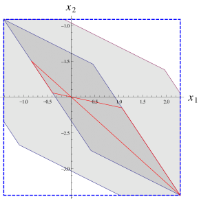
Figure 1: The united parametric solution set of the system (13) (the most inner butterfly region with red boundary), its interval enclosure (14) (dashed line box), the $p,l$-solution (light gray polytope) and the newly proposed p-solution (dark gray polytope).

Example 2.

Consider the interval parametric linear system

$$\begin{pmatrix}-1+\frac{1}{2}p_{2}-2p_{3}&-1-\frac{1}{2}p_{2}\\ -1-p_{2}&-1+p_{2}\end{pmatrix}x=\begin{pmatrix}p_{2}+3p_{1}-1\\ -2p_{2}+2p_{1}+3\end{pmatrix},\\ p_{1}\in[-\frac{1}{4},1],\;p_{2}\in[\frac{1}{2},\frac{3}{2}],\;p_{3}\in[\frac{1}{5},\frac{2}{3}].$$ (17)

For this system both conditions (3) and (7) are satisfied. The method from Theorem 2 yields interval vector

$$\left([-5.725,3.975],[-9.0805\ldots 5,9.175]\right)^{\top}$$

and a parameterized solution enclosure

$$x^{\prime}(p,l)=\begin{pmatrix}-\frac{7}{8}\\ \frac{17}{360}\end{pmatrix}+\begin{pmatrix}-\frac{11881p_{1}}{8400}+\frac{3124703p_{2}}{1512000}\\ -\frac{3969p1}{2200}-\frac{168057p_{2}}{44000}+\frac{1701p_{3}}{880}\end{pmatrix}+\begin{pmatrix}\frac{1108559}{378000}l_{1}\\ \frac{1116613}{198000}l_{2}\end{pmatrix},\\ p_{1}\in[-\frac{5}{8},\frac{5}{8}],\;p_{2}\in[-\frac{1}{2},\frac{1}{2}],\;l_{1},l_{2}\in[-1,1].$$

The equivalent optimal rank one representation of system (17) is obtained for

$$L=\begin{pmatrix}1&\frac{1}{2}\\ 0&-1\end{pmatrix},\;R=\begin{pmatrix}-2&0\\ 1&-1\end{pmatrix},\;D_{p}=\begin{pmatrix}p_{3}&0\\ 0&p_{2}\end{pmatrix},\\ F=\begin{pmatrix}3\\ 2\end{pmatrix},\;t=(0,2)^{\top}.$$

The interval parametric equation (8) has the form

$$\begin{pmatrix}1&p_{2}\\ -\frac{2}{3}p_{3}&1-\frac{58}{45}p_{2}\end{pmatrix}y=\begin{pmatrix}\frac{7}{4}-2p_{1}+2p_{2}\\ -\frac{83}{90}-\frac{4}{45}p_{1}-\frac{116}{45}p_{2}\end{pmatrix},\\ p_{1}\in[-\frac{5}{8},\frac{5}{8}],\;p_{2}\in[-\frac{1}{2},\frac{1}{2}],\;p_{3}\in[-\frac{7}{30},\frac{7}{30}].$$

An interval enclosure of the solution set of the last equation is

$$\mathbf{y}=\left([-5.7,9.2],[-10.4,77/9]\right)^{\top}.$$

Then, by Corollary 1, the parameterized solution is

$$x^{\prime\prime}(p)=\begin{pmatrix}-\frac{7}{8}\\ \frac{17}{360}\end{pmatrix}+\begin{pmatrix}1\\ \frac{49}{45}\end{pmatrix}p_{1}+\begin{pmatrix}0&\frac{31}{5}\\ -\frac{92}{15}&-\frac{2201}{225}\end{pmatrix}\begin{pmatrix}p_{3}\\ p_{2}\end{pmatrix},\\ p_{1}\in[-\frac{5}{8},\frac{5}{8}],\;p_{2}\in[-\frac{1}{2},\frac{1}{2}],\;p_{3}\in[-\frac{7}{30},\frac{7}{30}].$$

The two parameterized solutions and their interval hulls are presented and compared in Figure 2.

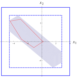
Figure 2: Left: The united parametric solution set of the system (17) (the most inner region with red boundary), its interval enclosure by Theorem 3 (dashed line box), and the interval enclosure by Theorem 2 (the outer solid line box). Right: The united parametric solution set of the system (17) (the most inner region with red boundary), the parameterized solution $x^{\prime\prime}(p)$ in gray and the parameterized solution $x^{\prime}(p,l)$ represented by its boundary.

In general, when comparing the two parameterized solutions $x(p,l)$ and $x(p_{\pi^{\prime\prime}},g)$, one has to consider the two relations $K+n\lesseqqgtr K+s-K_{1}$ and $x(\mathbf{p},\mathbf{l})\cong x(\mathbf{p}_{\pi^{\prime\prime}},\mathbf{g})$, where $\sim\in\{\subset,\supset\}$.

Example 3.

Consider the interval parametric linear system

$$\begin{pmatrix}\frac{1}{2}-p_{2}&p_{2}&2\\ p_{2}&-p_{2}&p_{1}\\ 2&p_{1}&-2+p_{1}\end{pmatrix}x=\begin{pmatrix}p_{2}\\ 2-p_{1}-p_{2}\\ p_{1}-1\end{pmatrix},\\ p_{1}\in[\frac{2}{3},\frac{4}{3}],\;p_{2}\in[\frac{1}{2},\frac{3}{2}].$$ (18)

For this system both conditions (3) and (7) are satisfied. The interval hull of the united parametric solution set, rounded outwardly and presented by $6$ digits in the mantissa, is

$$\left([-.156997,.363637],[-.727273,.5972697],[.1896562,.4927185]\right)^{\top}.$$

The method from Theorem 2 yields interval vector

$$\left([-.782941,.782941],[-1.014773,1.6814392],[.082439,.584226]\right)^{\top}$$

and a parameterized solution enclosure

$$x^{\prime}(p,l)=\begin{pmatrix}0\\ \frac{1}{3}\\ \frac{1}{3}\end{pmatrix}+\begin{pmatrix}-0.38474p_{1}-0.256493p_{2}\\ 0.924365p_{1}+0.728287p_{2}\\ -0.392728p_{1}+0.0374027p_{2}\end{pmatrix}+\begin{pmatrix}0.526447l_{1}\\ 0.67584l_{2}\\ 0.101283l_{3}\end{pmatrix},\\ p_{1}\in[-\frac{1}{3},\frac{1}{3}],\;p_{2}\in[-\frac{1}{2},\frac{1}{2}],\;l_{1},l_{2},l_{3}\in[-1,1].$$ (19)

The coefficient matrix of $p_{2}$ has rank one, while the coefficient matrix of $p_{1}$ has rank two. Therefore, the equivalent optimal rank one representation of system (18) is obtained for

$$D_{p}=\begin{pmatrix}p_{1}&0&0\\ 0&p_{1}&0\\ 0&0&p_{2}\end{pmatrix},\;L=\begin{pmatrix}0&0&-1\\ 0&1&1\\ 1&1&0\end{pmatrix},\;R=\begin{pmatrix}0&1&0\\ 0&0&1\\ 1&-1&0\end{pmatrix},\\ t=(2,-1,-1)^{\top}.$$

By Theorem 4, the parameterized solution is

$$x^{\prime\prime}(p,g)=\begin{pmatrix}0\\ \frac{1}{3}\\ \frac{1}{3}\end{pmatrix}+\left(\check{A}^{-1}L\right)\begin{pmatrix}p_{1}&0&0\\ 0&g&0\\ 0&0&p_{2}\end{pmatrix}\begin{pmatrix}2.79556\\ 1.56338\\ 2.249\end{pmatrix},\\ p_{1},g\in[-\hat{p}_{1},\hat{p}_{1}]={[}-\frac{1}{3},\frac{1}{3}{]},\;p_{2}\in{[}-\frac{1}{2},\frac{1}{2}{]}.$$ (20)

Its interval evaluation $x^{\prime\prime}(\mathbf{p},\mathbf{g})$ is

$$\left([-1.032869,1.032869],[-.795558,1.462224],[.1032854,.5633813]\right)^{\top}.$$

For this example $x^{\prime\prime}(p,g)$ involves less number of interval parameters than $x^{\prime}(p,l)$, however $x_{1}^{\prime\prime}(\mathbf{p},\mathbf{g})\supset x_{1}^{\prime}(\mathbf{p},\mathbf{l})$. The latter disadvantage may vanish when enclosing some secondary variables, see Example 5.

5 Bounding secondary (derived) variables

In this section we present a new application direction for the parameterized solution enclosures and demonstrate the value of the newly proposed parameterized solution. Before discussing practical applications in structural mechanics, we make some general remarks.

Remark 1.

Since $x(\mathbf{p}_{\pi^{\prime\prime}},\mathbf{g})$ in Theorem 4 is considered as a natural interval extension of the function $x(p)$, $p\in[-\hat{p},\hat{p}]$ in (11), one has to be careful when enclosing secondary variables $z(p,x(p_{\pi^{\prime\prime}},g))$, where $x(p_{\pi^{\prime\prime}},g))$ is obtained by Theorem 4. In the general case, the enclosure of the latter should be done by computing the natural interval extension of $z(p,x(p))$, where $x(p)$ is the function in (11), see Example 4.

Example 4.

Consider a linear system which satisfies the requirements of Corollary 1 and has a parameterized solution enclosure

$$x(p^{\prime})=\check{x}+Up^{\prime},\quad p^{\prime}\in[-\hat{p},\hat{p}],$$ (21)

where $p^{\prime}=(p_{\pi^{\prime}}^{\top},p_{\pi^{\prime\prime}}^{\top})^{\top}$ and $U\in\mathbb{R}^{n\times K}$ is the matrix that makes equivalent the above representation and the representation (12). With the additional requirements $K=n$ and non-singularity of $U$, consider the secondary variables

$$z(p^{\prime})=U^{-1}x(p^{\prime})-p^{\prime},\quad p^{\prime}\in[-\hat{p},\hat{p}].$$ (22)

Replacing $x(p^{\prime})$ form (21) in $z(p^{\prime})$ we obtain

$$z(p^{\prime}) = U^{-1}\check{x}+p^{\prime}-p^{\prime}$$ (23)

$$= U^{-1}\check{x}.$$ (24)

Due to the multiple occurrence of the parameters $p^{\prime}$ in $z(p^{\prime})$ and according to Remark 1, interval enclosure of the variables $z$ should be obtained as a natural interval extension of $z(p^{\prime})$ in (22) or in (23) but not by $z(p^{\prime})$ in (24), which is not an interval function.

Remark 2.

Let $z(p,x(p_{\pi^{\prime\prime}},g))$, where $x(p_{\pi^{\prime\prime}},g))$ is obtained by Theorem 4, be $z(p,x(p_{\pi^{\prime\prime}},g))=Bx(p_{\pi^{\prime\prime}},g)=Bx(p)$, where $x(p)$ is the function in (11). Denote $V=CLD_{|\mathbf{y}-t|}$. Then, the natural interval extension of

$$Bx(p)=B\check{x}+\left(BCF\right)p_{\pi^{\prime\prime}}+\left(BV\right)g(p_{\pi^{\prime}})$$

is equal to the range of

$$Bx(p_{\pi^{\prime\prime}},g)=B\check{x}+\left(BCF\right)p_{\pi^{\prime\prime}}+\left(BV\right)g.$$

Example 5.

Consider the system from Example 3 and the obtained two parameterized solution enclosures $x^{\prime}(p,l)$ and $x^{\prime\prime}(p,g)$. Find interval enclosures of the secondary variables $z=Bx$, where $x$ is every one of the two parameterized solution enclosures, and $B=\begin{pmatrix}1&2&3\\ 3/2&1&2\\ 1/2&1/2&1\end{pmatrix}$. With $x^{\prime}(p,l)$ in (19) and the notation (4), we obtain

$$z\left(B,x^{\prime}(p,l)\right) = B\tilde{x}+(BV)p^{\prime}+(B\hat{l})l$$

$$\in \mathbf{z}^{\prime}=\left([-1.2667226,4.6000559],[-1.0233198,3.02331978],\right.$$

$$\hskip 144.54pt\left.[-.38004820,1.3800482]\right)^{\top}.$$

With $x^{\prime\prime}(p,g)$ in (20) we obtain

$$z\left(B,x^{\prime\prime}(p,g)\right)\in\mathbf{z}^{\prime\prime}=\left([-1.0222306,4.3555640],\right.\\ \left.[-.69090480,2.6909048],[-.27465195,1.2746520]\right)^{\top}.$$

The percentage by which $\mathbf{z}^{\prime}$ overestimates $\mathbf{z}^{\prime\prime}$ is $\left(8,16,12\right)^{\top}$%.

In what follows we consider finite element (FE) models in linear elastic structural mechanics involving interval uncertainties in material and load parameters. The interval models are based on classical interval arithmetic. While various methods and techniques are devised for obtaining very sharp (even the exact) bounds for the unknowns (e.g., displacements, called primary variables) of an interval parametric linear system, obtaining sharp enclosure of the so-called derived (secondary) variables (as axial forces, strains or stresses) is referred in [14] as a challenging problem. Secondary (derived) variables are functions of the primary variables or of both primary variables and the initial interval model parameters. Due to the dependency, the derived quantities are obtained with significant overestimation. Some special techniques are usually applied to decrease the overestimation in the secondary quantities. In [14] a new mixed formulation of interval finite element method (IFEM) is proposed, where both primary and derived quantities of interest are involved as primary variables in an expanded interval parametric linear system. In this section we propose an alternative approach based on the newly proposed parameterized solution. The new approach requires that the interval enclosure of the primary variables is obtained as a parameterized solution. Thus, interval estimation of the secondary variables reduces to range enclosure of the expressions representing secondary variables as functions of the initial interval model parameters. In formal notations the approach we propose, based on the new parameterized solution of primary variables, is presented as follows.

Let $A(p)u=a(p)$, $p\in\mathbf{p}$, be an interval parametric linear system for the primary variables $u$ and $p\in\mathbf{p}$ be the interval model parameters. For simplicity of the presentation we assume that the coefficient matrices of all interval parameters have rank one and the system for the primary variable can be solved by Theorem 3. Depending on which material parameters are considered as interval ones, an element secondary variable is usually presented as $v=p_{i}b^{\top}u$, where $p_{i}$ is one of the interval material parameters and $b$ is a numerical vector. Algorithm 1 presents the new approach based on the newly proposed parameterized enclosure of the displacements as primary variables.

Algorithm 1.

Interval enclosure of the secondary variable $v$ obtained by the new parameterized enclosure (Corollary 1) of the primary variables $u$.

Input: numerical matrices $A_{0}\in\mathbb{R}^{n\times n}$, $L,R^{\top}\in\mathbb{R}^{n\times K}$, $F\in\mathbb{R}^{n\times(K-K_{1})}$ and vectors $a_{0}\in\mathbb{R}^{n}$, $t\in\mathbb{R}^{K}$ providing an equivalent representation (5); vectors $b\in\mathbb{R}^{n}$ and $\mathbf{p}\in\mathbb{IR}^{K}$.

Output: interval $\mathbf{v}=[v^{-},v^{+}]$ for the unknown secondary variable.

1. Obtain the new parameterized interval enclosure of the primary variables by Corollary 1

   $$u(p^{\prime})=u_{0}+Up^{\prime},\quad p^{\prime}\in[-\hat{p},\hat{p}],\qquad u_{0}\in\mathbb{R}^{n},U\in\mathbb{R}^{n\times K}.$$

   There is a flexibility in the implementation of this step of the algorithm, which is discussed in [8].

2. Generate $\mathbf{p}^{\prime}=[-\hat{p},\hat{p}]$,  $\mathbf{v}^{\prime}=\left(\check{p}_{i}+\mathbf{p}_{i}^{\prime}\right)\left(b^{\top}u_{0}+(b^{\top}U)\mathbf{p}^{\prime}\right)$.

3. Since $v^{\prime}(p^{\prime})$ is a quadratic function of $p_{i}^{\prime}$, $\mathbf{v}^{\prime}$ may overestimate the true range $\square\{v^{\prime}(p^{\prime})\mid p^{\prime}\in\mathbf{p}^{\prime}\}$. To reduce the overestimation we may prove if this range is attained at some endpoints of $\mathbf{p}_{i}^{\prime}$. To this end we evaluate

   $$\frac{\partial v^{\prime}(p^{\prime})}{\partial p_{i}^{\prime}}=b^{\top}u(p^{\prime})+p_{i}b^{\top}\frac{\partial u(p^{\prime})}{\partial p_{i}^{\prime}}\in\left(b^{\top}u_{0}+(b^{\top}U)\mathbf{p}^{\prime}\right)+\mathbf{p}_{i}\left(b^{\top}U_{\bullet i}\right).$$

   Evaluate $\mathbf{v}_{1}=[v_{1}^{-},v_{1}^{+}]=b^{\top}u_{0}+(b^{\top}U)\mathbf{p}^{\prime}$ and $\mathbf{v}_{2}=\mathbf{p}_{i}(b^{\top}U_{\bullet i})$.

   1. If $0\in v_{1}^{-}+\mathbf{v}_{2}$, then $v^{-}=(\mathbf{v}^{\prime})^{-}$
                                 else   $s_{1}={\rm sign}(v_{1}^{-}+\mathbf{v}_{2})\in\{-1,1\}$;
                                          $(\mathbf{p}^{\prime})_{i}=-s_{1}\hat{p}_{i}$;
                                          $v^{-}=(\check{p}_{i}-s_{1}\hat{p}_{i})(b^{\top}u_{0}+(b^{\top}U)\mathbf{p}^{\prime})$;

   2. If $0\in v_{1}^{+}+\mathbf{v}_{2}$, then $v^{+}=(\mathbf{v}^{\prime})^{+}$
                                 else   $s_{2}={\rm sign}(v_{1}^{+}+\mathbf{v}_{2})\in\{-1,1\}$;
                                          $(\mathbf{p}^{\prime})_{i}=s_{2}\hat{p}_{i}$;
                                          $v^{+}=(\check{p}_{i}+s_{1}\hat{p}_{i})(b^{\top}u_{0}+(b^{\top}U)\mathbf{p}^{\prime})$;

4. Return $\mathbf{v}=[v^{-},v^{+}]$.

Lemma 1.

Let $f(x):\mathbf{x}\subset\mathbb{IR}^{m}\rightarrow\mathbb{IR}^{n}$ be an interval function such that each component $f_{i}(x):\mathbf{x}\subset\mathbb{IR}^{m}\rightarrow\mathbb{IR}$ is a linear function of all interval variables except one $x_{j_{i}}$ and the interval variables $x_{i}$, $i\neq j_{i}$ appear only once in the expression of $f_{i}(x)$. Then, for every $\tilde{x}\in\mathbf{x}$ and every $1\leq i\leq n$ there exist $x_{j_{i}}^{\prime},x_{j_{i}}^{\prime\prime}\in\mathbf{x}_{j_{i}}$ such that

$$f_{i}(\mathbf{x}^{\prime})\leq f_{i}(\tilde{x})\leq f_{i}(\mathbf{x}^{\prime\prime}),$$ (25)

where $\mathbf{x}^{\prime}_{i}=\mathbf{x}_{i}^{\prime\prime}=\mathbf{x}_{i}$, $i\neq j_{i}$, $\mathbf{x}^{\prime}_{j_{i}}=x_{j_{i}}^{\prime}$, $\mathbf{x}^{\prime\prime}_{j_{i}}=x_{j_{i}}^{\prime\prime}$.

Theorem 7.

Algorithm 1 provides interval enclosure of a secondary variable $v$ with quality, which is not worse than the quality of the enclosure of primary variables $u$ obtained by Corollary 1 (Theorem 3) if steps 3.1 and 3.2 go to their else-clause.

Proof.

It is obvious that the natural interval extension $\mathbf{v}^{\prime}=v^{\prime}(\mathbf{p}^{\prime})$ of $v^{\prime}(p^{\prime})=$ $\left(\check{p}_{i}+p_{i}^{\prime}\right)\left(b^{\top}u_{0}+(b^{\top}U)p^{\prime}\right)$ contains the true range of the secondary variable $v$. Basing on Lemma 1, steps 3.1 and 3.2 of the algorithm try to prove if some endpoint of $\mathbf{p}_{i}^{\prime}$ generates the lower, respectively the upper, endpoint of the true range of $v^{\prime}(p^{\prime})$. Then, the sign of the intervals $v_{1}^{-}+\mathbf{v}_{2}$, respectively $v_{1}^{+}+\mathbf{v}_{2}$, will determine that. Let step $3$ of the algorithm give the true range of $v^{\prime}(p^{\prime})$ on $p^{\prime}\in\mathbf{p}^{\prime}$, that is $[v^{-},v^{+}]=\square\{v^{\prime}(p^{\prime})\mid p^{\prime}\in\mathbf{p}^{\prime}\}$. We have that $v^{\prime}(p^{\prime})$ is a function of $u(p^{\prime})$ and $u(\mathbf{p}^{\prime})$ is an outer interval enclosure of $u(p^{\prime})$, $p^{\prime}\in\mathbf{p}^{\prime}$, obtained by some numerical method. Therefore, $[v^{-},v^{+}]$ is an outer interval enclosure of the secondary variable $v$ and the quality of this enclosure depends of the quality of the enclosure $u(\mathbf{p}^{\prime})$. ∎

For enclosing the derived variables considered in IFEMs of mechanical structures it is essential that the parameterized representation of the primary variables involves only the initial interval parameters and their number is less than the number of interval parameters in the parameterized solutions $x(p,l)$. In Section 5.1, the parameterized solution obtained by Theorem 2 is representative of all parameterized solutions $x(p,l)$ ([1]–[6]) which satisfy Theorem 6.

5.1 Truss Example 1

Consider a $6$-bar truss structure as presented in Fig. 3 after [16]. The structure consists of $6$ elements. The crisp values of the parameters of the truss are presented in Table 1.

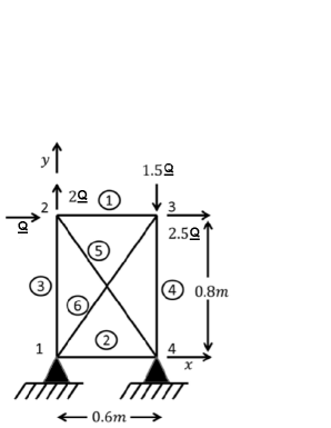
Figure 3: A $6$-bar truss structure after [16].

Parameter	Value
Modulus of elasticity for all elements   .
$E_{i}$, $i=1,\ldots,6$ ($kN/m^{2}$)	$2.1\times 10^{8}$
Cross sectional area
$A_{1},A_{2},A_{3},A_{4}$ ($m^{2}$)	$1.0\times 10^{-3}$
Cross sectional area
$A_{5},A_{6}$ ($m^{2}$)	$1.05\times 10^{-3}$
Load $Q$ ($kN$)	$20.5$
Length of the first and second element
$L_{1},L_{2}$ ($m$)	$0.6$
Length of the third and fourth element
$L_{3},L_{4}$ ($m$)	$0.8$
Length of the fifth and sixth element
$L_{6},L_{6}$ ($m$)	$1$

Table 1: Crisp values of the parameters for the $6$-bar truss structure.

The traditional finite element method (FEM) for this structure leads to a linear system

$$K(E,A,L)u=f(Q),$$

where $K(E,A,L)$ is the reduced stiffness matrix depending on the structural parameters (modulus of elasticity $E$, cross sectional area $A$, length $L$) for each element, $f(Q)$ is the load vector and $u$ is the displacement vector. Namely,

$$K(E,A,L)\;=\\ \begin{pmatrix}\frac{E_{1}A_{1}}{L_{1}}+0.36\frac{E_{5}A_{5}}{L_{5}}&-0.48\frac{E_{5}A_{5}}{L_{5}}&-\frac{E_{1}A_{1}}{L_{1}}&0\\ -0.48\frac{E_{5}A_{5}}{L_{5}}&\frac{E_{3}A_{3}}{L_{3}}+0.64\frac{E_{5}A_{5}}{L_{5}}&0&0\\ -\frac{E_{1}A_{1}}{L_{1}}&0&\frac{E_{1}A_{1}}{L_{1}}+0.36\frac{E_{6}A_{6}}{L_{6}}&0.48\frac{E_{6}A_{6}}{L_{6}}\\ 0&0&0.48\frac{E_{6}A_{6}}{L_{6}}&\frac{E_{4}A_{4}}{L_{4}}+0.64\frac{E_{6}A_{6}}{L_{6}}\end{pmatrix},\\[6.0pt] f(Q)\;=\;(Q,2Q,2.5Q,-1.5Q)^{\top},\qquad\qquad u=(ux_{2},uy_{2},ux_{3},uy_{3})^{\top}.$$ (26)

Let the load parameter $Q$ be unknown-but-bounded in the interval $\mathbf{Q}=[20,21]kN$ and the cross sectional areas $A_{5}$, $A_{6}$ be also uncertain varying in the intervals $[1.008,1.092]\times 10^{-3}$ $m^{2}$, $[1,1.1]\times 10^{-3}$ $m^{2}$, respectively. The aim is to obtain interval enclosure for the displacements (as primary variables depending on interval model parameters) and for the element axial forces (as secondary variables). Axial forces are quantities of practical interest in design. For the considered example, the global force vector $F=(F_{e_{1}},F_{e_{3}},F_{e_{4}},F_{e_{5}},F_{e_{6}})^{\top}$ is determined by $F=D_{v}Tu$, where $F_{e_{i}}$ are the corresponding element forces and

$$v=\left(\frac{E_{1}A_{1}}{L_{1}},\frac{E_{3}A_{3}}{L_{3}},\frac{E_{4}A_{4}}{L_{4}},\frac{E_{5}A_{5}}{L_{5}},\frac{E_{6}A_{6}}{L_{6}}\right)^{\top},\quad T=\begin{pmatrix}-1&0&1&0\\ 0&1&0&0\\ 0&0&0&1\\ -\frac{6}{10}&\frac{8}{10}&0&0\\ 0&0&\frac{8}{10}&\frac{6}{10}\end{pmatrix}.$$

Above, the displacements $u=u(A_{5},A_{6},Q)$ (as primary variables), the vector $v=v(A_{5},A_{6})$ and the secondary variables – element axial forces $F_{e_{i}}$, $i=1,3,4,5,6$ – are functions of the interval model parameters $A_{5},A_{6},Q$.

First, we find interval enclosures for the displacements as parameterized solutions to the interval parametric linear system $K(A_{5},A_{6})u=f(Q)$. Applying Theorem 2 we obtain

$$10^{4}u^{\prime}(A_{5},A_{6},Q,l)\approx\\ \begin{pmatrix}8.5846-2153.0A_{5}-2134.2A_{6}+.41896Q+10^{-3}26.693l_{1}\\ 3.2669+491.791A_{5}-559.409A_{6}+.15937Q+10^{-3}6.6039l_{2}\\ 8.9579-1876.6A_{5}-2449.5A_{6}+.43727Q+10^{-3}26.952l_{3}\\ -3.1109+491.80A_{5}-559.420A_{6}+.15176Q+10^{-3}6.6017l_{4}\end{pmatrix},$$

where $A_{i}\in[-\hat{A}_{i},\hat{A}_{i}]$, $i=5,6$, $Q\in[-\hat{Q},\hat{Q}]$, $l_{i}\in[-1,1]$, $i=1,\ldots,4$. Its interval hull is

$$10^{4}u^{\prime}(\mathbf{A}_{5},\mathbf{A}_{6},\mathbf{Q},\mathbf{l})\subset\\ \left([8.151,9.018],[3.131,3.402],[8.511,9.405],[-3.242,-2.979]\right)^{\top}.$$

With the crisp values from Table 1, the optimal equivalent rank one representation of the system (26) is $(A_{0}+LD_{g}R)u=f(Q)$, where $g=(A_{5},A_{6})^{\top}$ and

$$10^{-5}A_{0}=\begin{pmatrix}\frac{7}{2}&0&-\frac{7}{2}&0\\ 0&\frac{21}{8}&0&0\\ -\frac{7}{2}&0&\frac{7}{2}&0\\ 0&0&0&\frac{21}{8}\end{pmatrix},\;10^{-5}L=\begin{pmatrix}756&0\\ -1008&0\\ 0&756\\ 0&1008\end{pmatrix},\;R^{\top}=\begin{pmatrix}1&0\\ -\frac{4}{3}&0\\ 0&1\\ 0&\frac{4}{3}\end{pmatrix}.$$

The application of Corollary 1 to the above system yields the parameterized solution

$$10^{4}u^{\prime\prime}(A_{5},A_{6},Q)\approx\begin{pmatrix}8.5846+2306.60A_{5}+2285.45A_{6}-.41876Q\\ 3.2669-527.104A_{5}+599.307A_{6}-.15936Q\\ 8.9579+2010.11A_{5}+2622.56A_{6}-.43697Q\\ -3.1109-527.104A_{5}+599.307A_{6}+.15175Q\end{pmatrix},$$

where $A_{i}\in[-\hat{A}_{i},\hat{A}_{i}]$, $i=5,6$, $Q\in[-\hat{Q},\hat{Q}]$. Its interval hull is

$$10^{4}u^{\prime\prime}(\mathbf{A}_{5},\mathbf{A}_{6},\mathbf{Q})\subset\left([8.164,9.006],[3.135,3.399],\right.\\ \left.[8.523,9.392],[-3.239,-2.982]\right)^{\top}.$$

It is readily seen that $u^{\prime\prime}(\mathbf{A}_{5},\mathbf{A}_{6},\mathbf{Q})$ provides sharper interval enclosure to the displacements than $u^{\prime}(\mathbf{A}_{5},\mathbf{A}_{6},\mathbf{Q},\mathbf{l})$. Percentage by which the latter overestimates the former is $(2.95,2.32,2.87,2.39)^{\top}$. This implies that the newly proposed parameterized solution $u^{\prime\prime}(A_{5},A_{6},Q)$ will provide a sharper enclosure of the element axial forces.

For the particular example we have

$$10^{-5}D_{v}T = 10^{-5}D_{v^{\prime}}T^{\prime}$$

$$= 10^{-5}D_{v^{\prime}}\begin{pmatrix}-\frac{7}{2}&0&\frac{7}{2}&0\\ 0&\frac{21}{8}&0&0\\ 0&0&0&\frac{21}{8}\\ -1260&1680&0&0\\ 0&0&1680&1260\end{pmatrix},\;v^{\prime}=\begin{pmatrix}1\\ 1\\ 1\\ A_{5}\\ A_{6}\end{pmatrix},$$

which shows that the element axial forces $F_{e_{i}}$, $i=1,3,4$, are linear functions of the interval model parameters $A_{5},A_{6},Q$, while the axial forces $F_{e_{5}},F_{e_{6}}$ are quadratic functions of the interval parameters $A_{5},A_{6}$, respectively. In what follows, in particular Table 2, we use the notation

$$\begin{split}&u^{\prime}(A_{5},A_{6},Q,l)=x^{\prime}_{0}+B^{\prime}(A_{5},A_{6},Q)^{\top}+C^{\prime}l,\quad l\in\mathbf{l}=([-1,1],\ldots,[-1,1])^{\top},\\ &u^{\prime\prime}(A_{5},A_{6},Q)=x^{\prime\prime}_{0}+B^{\prime\prime}(A_{5},A_{6})^{\top}+C^{\prime\prime}(Q),\\ &\mathbf{u}^{\prime}=u^{\prime}(\mathbf{A}_{5},\mathbf{A}_{6},\mathbf{Q},\mathbf{l}),\qquad\mathbf{u}^{\prime\prime}=u^{\prime\prime}(\mathbf{A}_{5},\mathbf{A}_{6},\mathbf{Q}),\\ &\mathbf{F}^{\prime}=D_{\mathbf{v}^{\prime}}(T^{\prime}\mathbf{u}^{\prime}),\qquad\mathbf{F}^{\prime\prime}=D_{\mathbf{v}^{\prime}}(T^{\prime}\mathbf{u}^{\prime\prime}),\qquad\qquad[\mp\hat{a}]=[-\hat{a},\hat{a}],\\ &F^{\prime}(\mathbf{A}_{5},\mathbf{A}_{6},\mathbf{Q},\mathbf{l})=D_{\mathbf{v}^{\prime}}\left(T^{\prime}x^{\prime}_{0}+(T^{\prime}B^{\prime})([\mp\hat{A}_{5}],[\mp\hat{A}_{6}],[\mp\hat{Q}])^{\top}+T^{\prime}\mathbf{l}\right),\\ &F^{\prime\prime}(\mathbf{A}_{5},\mathbf{A}_{6},\mathbf{Q})=D_{\mathbf{v}^{\prime}}\left(T^{\prime}x^{\prime\prime}_{0}+(T^{\prime}B^{\prime\prime})([\mp\hat{A}_{5}],[\mp\hat{A}_{6}])^{\top}+(T^{\prime}C^{\prime\prime})([\mp\hat{Q}])\right),\end{split}$$

where $x^{\prime}_{0}$, $B^{\prime}$, $C^{\prime}$ are numerical vector and matrices presented in $u^{\prime}(A_{5},A_{6},Q,l)$ above, and $x^{\prime\prime}_{0}$, $B^{\prime\prime}$, $C^{\prime\prime}$ are numerical vector and matrices presented in the numerical expression of $u^{\prime\prime}(A_{5},A_{6},Q,l)$ above. Table 2 presents and compares interval enclosures of the element axial forces $\mathbf{F}^{\prime},\mathbf{F}^{\prime\prime}$, obtained via direct interval computation, and the enclosures $F^{\prime}(\mathbf{A}_{5},\mathbf{A}_{6},\mathbf{Q},\mathbf{l})$, $F^{\prime\prime}(\mathbf{A}_{5},\mathbf{A}_{6},\mathbf{Q})$, obtained via the two kinds parameterized solutions $u^{\prime}(A_{5},A_{6},Q,l)$ and $u^{\prime\prime}(A_{5},A_{6},Q)$, respectively.

	$\mathbf{F}^{\prime}=$	$\mathbf{F}^{\prime\prime}$	$F^{\prime\prime}(\mathbf{A}_{5},\mathbf{A}_{6},\mathbf{Q})$
	$F^{\prime}(\mathbf{A}_{5},\mathbf{A}_{6},\mathbf{Q},\mathbf{l})$
$e_{1}$	[-17.740, 43.875]	[-16.843, 42.978]	[11.722, 14.412]
$e_{3}$	[82.215, 89.298]	[82.297, 89.216]	[82.297, 89.216]
$e_{4}$	[-85.102, -78.218]	[-85.020, -78.300]	[-85.019, -78.300]
$e_{5}$	[-66.621, -45.919]	[-66.388, -46.135]	[-62.365, -49.848]
$e_{6}$	[102.13, 132.51]	[102.39, 132.23]	[104.86, 129.51]

Table 2: Interval enclosures for the element axial forces in the $6$-bar truss structure obtained via the two kinds of parameterized solutions.

Due to $\mathbf{u}^{\prime\prime}\subset\mathbf{u}^{\prime}$, it is clear that $\mathbf{F}^{\prime\prime}\subset\mathbf{F}^{\prime}$ and the latter overestimation is $(2.9,2.3,2.4,2.2,1.8)^{\top}$%. Note that the enclosures $\mathbf{F}^{\prime},\mathbf{F}^{\prime\prime}$ are so bad that the sign of $F_{e_{1}}$ cannot be determined. Note also that $F^{\prime}(\mathbf{A}_{5},\mathbf{A}_{6},\mathbf{Q},\mathbf{l})=\mathbf{F}^{\prime}$. The latter means that Kolev-style parameterized solution was not able to improve the bounds $\mathbf{F}^{\prime}$. Intervals $\mathbf{F}^{\prime\prime}$ overestimate intervals $F^{\prime\prime}(\mathbf{A}_{5},\mathbf{A}_{6},\mathbf{Q})$ by $(95.5,0,0,38.2,17.4)^{\top}$%, respectively. Since $F_{e_{i}}(A_{5},A_{6},Q)$, $i=5,6$, are quadratic polynomials of the interval parameters $A_{5}$, $A_{6}$, (represented by a $v^{\prime}$ in Algorithm 1) respectively, their interval values presented in Table 2, in general, may not be equal to the corresponding ranges. Evaluating partial derivatives as presented in Algorithm 1, we prove that $F_{e_{5}}^{\prime\prime}(A_{5},A_{6},Q)$ is monotonic decreasing on $A_{5}$, while $F_{e_{6}}^{\prime\prime}(A_{5},A_{6},Q)$ is monotonic increasing on $A_{6}$. Thus $F^{\prime\prime}(\mathbf{A}_{5},\mathbf{A}_{6},\mathbf{Q})$ presented in Table 2 are the exact ranges of the corresponding expressions of $v^{\prime}$ and the quality of the enclosures $F^{\prime\prime}(\mathbf{A}_{5},\mathbf{A}_{6},\mathbf{Q})$ is the same as the quality of the enclosures $\mathbf{u}^{\prime\prime}$. Note that neither $\mathbf{u}^{\prime\prime}$ nor $F^{\prime\prime}(\mathbf{A}_{5},\mathbf{A}_{6},\mathbf{Q})$ are the exact ranges of the corresponding unknowns, see the proof of Theorem 7. In order to demonstrate the quality of the enclosures $F^{\prime\prime}(\mathbf{A}_{5},\mathbf{A}_{6},\mathbf{Q})$ we give below the corresponding exact ranges rounded outwardly

$$F\in\left([11.8215,14.3755],[82.4287,89.1673],[-84.9499,-78.4121],\right.\\ \left.[-58.9591,-53.0358],[109.960,123.970]\right)^{\top}.$$

5.2 Truss Example 2

Consider a finite element model of a one-bay $20$-floor truss cantilever presented in Fig. 4, after [17].

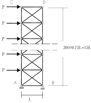
Figure 4: One-bay $20$-floor truss cantilever after [17].

The structure consists of 42 nodes and 101 elements. The bay is $L=1$m, every floor is $0.75L$, the element cross-sectional area is $A=0.01$ m², and the crisp value for the element Young modulus is $E=2\times 10^{8}$kN/m². Twenty horizontal loads with nominal value $P=10$ kN are applied at the left nodes. The boundary conditions are determined by the supports: at $A$ the support is a pin, at $B$ the support is roller. It is assumed $10$% uncertainty in the modulus of elasticity $E_{k}$ of each element ($\mp 5$% from the corresponding mean value) and $10$% uncertainty in the twenty loads. The goal is to obtain bounds for the axial force ($F_{40}$) in element $40$.

Exactly this problem is used in [14] as a benchmark problem for the applicability, computational efficiency and scalability of the approach proposed therein for structures with complex configuration and a large number of interval parameters. The aim of using this example in the present work is similar: to check these properties for the newly proposed Algorithm 1 based on the new parameterized solution. In addition, the interval result obtained by the approach proposed here will be compared to the results obtained by various other approaches considered in [14, Example 2].

Table 3 presents intervals for the axial force $F_{40}$ in element $40$, which are obtained by:

• the special expanded finite element formulation, proposed in [14], ($\mathbf{F}_{40}$);

• the newly proposed parameterized solution and step 2 of Algorithm 1, ($F^{\prime}_{40}(\mathbf{E},\mathbf{P})$);

• the newly proposed parameterized solution and step 3 of Algorithm 1, ($F^{\prime\prime}_{40}(\mathbf{E},\mathbf{P})$).

$\mathbf{F}_{40}$ by [14]	$F^{\prime}_{40}(\mathbf{E},\mathbf{P})$	$F^{\prime\prime}_{40}(\mathbf{E},\mathbf{P})$
[60.652, 98.991]	[55.729, 106.03]	[61.595, 98.639]

Table 3: Axial force $F_{40}$ (kN) in element $40$ of the cantilever truss obtained by various approaches.

Interval values for the axial force $F_{40}$, obtained by Pownuk’s “gradient-free” method [18] and by the Neumaier’s enclosure $\mathbf{z}_{2}(u)$ [13, Eqn. (4.13)], are presented in [14] and can be compared.

It should be mentioned that the coefficient matrices of all interval parameters in the linear system for the displacements have rank one. Therefore, there are no exceed interval parameters in the parameterized solution enclosure for the displacements. The symbolic expression of $F_{40}(E,P)$ is a quadratic function of the interval parameter $E_{40}$. Applying step 3 of Algorithm 1 we prove numerically that both the lower and the upper bounds of $F_{40}(E,P)$ are attained at the upper bound of $\mathbf{E}_{40}$. Note that this does not mean monotonic dependence of $\mathbf{E}_{40}$. Note also that the above proof is very easy compared to proving monotonic dependence of the displacements on the interval parameters. Step 3 in Algorithm 1 costs nothing compared to step 2 of the algorithm. Thus, we obtain an improvement $F^{\prime\prime}_{40}(\mathbf{E},\mathbf{P})$ of the bounds $F^{\prime}_{40}(\mathbf{E},\mathbf{P})$ in Table 3. Interval $F^{\prime\prime}_{40}(\mathbf{E},\mathbf{P})$ is sharper than the interval $\mathbf{F}_{40}$, obtained by the approach of [14], which shows the efficiency of the newly proposed approach based on the new parameterized solution. It should be also mentioned that the interval axial force $\mathbf{z}_{2}(u)$, showed in [14, Table 4] and obtained by the Neumaier’s approach [13, Eqn. (4.13)], is the same as the interval $F^{\prime}_{40}(\mathbf{E},\mathbf{P})$ in Table 3.

6 Conclusion

We presented a new kind of parameterized solution to interval parametric linear systems. It is based on optimal rank one representation of the parameter dependencies. This representation determines the number of interval parameters in the parameterized solution, as well as, whether the new parameterized solution will have better properties than the Kolev-style parameterized solutions. The new parameterized solution possesses similar computational complexity as the corresponding numerical method of Theorem 3. Comparing to some parameterized solutions based on the weaker condition (3), the price we pay for a better solution depends on the difference between a matrix inversion, $O(s^{3})$, when solving equation (8) of dimension $s$ and the matrix inversion, $O(n^{3})$, related to most of the other methods. Note that in practical applications, where the new solution is most efficient, the dependencies have rank one structure and $s=K_{1}$. The newly proposed parameterized solution does not require affine arithmetic as most of the parameterized solutions considered in [5]. The required rank one representation of the parameter dependencies is usually inherited by the corresponding model in an application domain, see, e.g., [13]. Otherwise, one can use the matrix full rank factorization utilities provided by many general purpose computing environments.

The major advantage of the newly proposed parameterized solution is for interval parametric linear systems involving rank one uncertainty structure. Such systems appear often in various domain-specific models, cf., [12]. A general application direction is presented in this article and illustrated by some numerical examples originated from worst-case analysis of truss structures in mechanics.

While bounding secondary variables by the approach of [14] requires a dedicated IFEM formulation for each particular problem and the system to be solved is expanded by the number of derived quantities, the approach based on the new parameterized solution of primary variables does not depend on the IFEM formulation, does not require solving an expanded interval parametric linear system, and provides sharp bounds for the derived quantities by a simple interval evaluation. The proposed new approach could be applied for enclosing secondary variables in various other domains where the uncertainties have rank one structure.

References

- [1] L. Kolev, Parametrized solution of linear interval parametric systems, Appl. Math. Comput. 246 (2014) 229–246. https://doi.org/10.1016/j.amc.2014.08.037.
- [2] L. Kolev, A direct method for determining a -solution of linear parametric systems, J. Appl. Computat. Math. 5 (2016) 1–5. https://doi.org/10.4172/2168-9679.1000294.
- [3] L. Kolev, A class of iterative methods for determining p-solutions of linear interval parametric systems, Rel. Comput. 22 (2016) 26–46.
- [4] L. Kolev, P-solutions for a class of structured interval parametric systems, Preprint in Research Gate, 23 November 2018, submitted as the file “p-sol_struct_correct”. https://doi.org/10.13140/RG.2.2.14958.25921.
- [5] I. Skalna, Parametric Interval Algebraic Systems, Studies in Computational Intelligence 766, Springer (2018).
- [6] I. Skalna, M. Hladík, Direct and iterative methods for interval parametric algebraic systems producing parametric solutions, Numer. Linear Algebra Appl. (2019) e2229. https://doi.org/10.1002/nla.2229.
- [7] E.D. Popova, Parameterized outer estimation of AE-solution sets to parametric interval linear systems, Appl. Math. Comput. 311 (2017) 353–360. https://doi.org/10.1016/j.amc.2017.05.042.
- [8] E.D. Popova, Rank one interval enclosure of the parametric united solution set, BIT Numer. Math. 59 (2) (2019) 503–521. https://doi.org/10.1007/s10543-018-0739-4.
- [9] J. Rohn, Explicit inverse of an interval matrix with unit midpoint, Electronic Journal of Linear Algebra 22 (2011) 138–150. https://doi.org/10.13001/1081-3810.1430.
- [10] R. Piziak, P.L. Odell, Full rank factorization of matrices, Mathematics Magazine 72 (1999) 193–201.
- [11] E.D. Popova, Enclosing the solution set of parametric interval matrix equation , Numer. Algor. 78 (2018) 423–447. https://doi.org/10.1007/s11075-017-0382-1.
- [12] E.D. Popova, Improved enclosure for some parametric solution sets with linear shape, Computers and Mathematics with Applications 68 (2014) 994–1005. https://doi.org/10.1016/j.camwa.2014.04.005.
- [13] A. Neumaier, A. Pownuk, Linear systems with large uncertainties, with applications to truss structures, Rel. Comput. 13 (2007) 149–172. https://doi.org/10.1007/s11155-006-9026-1.
- [14] M.V. Rama Rao, R.L. Mullen, R.L. Muhanna, A new interval finite element formulation with the same accuracy in primary and derived variables, Int. J. Reliability and Safety 5 (2011) 336–357. https://doi.org/10.1504/IJRS.2011.041184.
- [15] R. B. Kearfott, Rigorous Global Search: Continuous Problems, Kluwer Academic Publishers (1996)
- [16] Z. Qiu, I. Elishakoff, Antioptimization of structures with large uncertain-but-non-random parameters via interval analysis, Computer Methods in Applied Mechanics and Engineering 152 (1998) 361–372. https://doi.org/10.1016/S0045-7825(96)01211-X.
- [17] R.L. Muhanna, Benchmarks for interval finite element computations, Center for Reliable Engineering Computing, Georgia Tech, USA, http://rec.ce.gatech.edu/resources/Benchmark_2.pdf, 2004 (accessed 12 November 2018).
- [18] A. Pownuk, N.K.G. Ramunigari, Design of 2D elastic structures with the interval parameters, Proceedings of 11th WSEAS International Mathematical and Computational Methods in Science and Engineering (MACMESE’09), Baltimore, MD, USA, 25-29 November 2009. http://www.wseas.us/e-library/conferences/2009/baltimore/MACMESE/MACMESE-01.pdf.