Acceleration of the tree method with SIMD instruction set

Abstract

We have developed a highly-tuned software library that accelerates the calculation of quadrupole terms in the Barnes-Hut tree code by use of a SIMD instruction set on the x86 architecture, Advanced Vector eXtensions 2 (AVX2). Our code is implemented as an extension of Phantom-GRAPE software library that significantly accelerates the calculation of monopole terms. If the same accuracy is required, the calculation of quadrupole terms can accelerate the evaluation of forces than that of only monopole terms because we can approximate gravitational forces from closer particles by quadrupole moments than by only monopole moments. Our implementation can calculate gravitational forces about 1.1 times faster in any system than the combination of the pseudoparticle multipole method and Phantom-GRAPE. Our implementation allows simulating homogeneous systems up to 2.2 times faster than that with only monopole terms, however, speed up for clustered systems is not enough because the increase of approximated interactions is insufficient to negate the increased calculation cost by computing quadrupole terms. We have estimated that improvement in performance can be achieved by the use of a new SIMD instruction set, AVX-512. Our code is expected to be able to accelerate simulations of clustered systems up to 1.08 times faster on AVX-512 environment than that with only monopole terms.

1 Introduction

Gravitational $N$-body simulations are widely used to study the nonlinear evolution of astronomical objects such as the large-scale structure in the universe, galaxy clusters, galaxies, globular clusters, star clusters and planetary systems.

Directly solving $N$-body problems requires the computational cost in proportion to $N^{2}$ and is unpractical for large $N$, where $N$ is the number of particles. Therefore, many ways to reduce the calculation cost have been developed. One of the sophisticated algorithms is the tree method ([Barnes & Hut (1986)]) that evaluates gravitational forces with calculation cost in proportion to $N\log{N}$. The tree method constructs a hierarchical oct-tree structure to represent a distribution of particles and approximates the forces from a distant group of particles by the multipole expansion. The opening parameter $\theta$ is used to determine the tradeoff between accuracy and performance. If $l/d<\theta$, forces from a group of particles are approximated by the multipole expansion, where $l$ is the spatial extent of the group and $d$ is the distance to the group. Thus, larger $\theta$ gives higher performance and less accuracy.

The tree method is also used with the Particle-Mesh (PM) method ([Hockney & Eastwood (1981)]) when the periodic boundary condition is applied. This combination is called as the TreePM method ([Xu (1995), Bagla (2002), Dubinski et al. (2004), Springel (2005), Yoshikawa & Fukushige (2005), Ishiyama et al. (2009), Ishiyama et al. (2012), Wang et al. (2018)]) that calculates the short-range force by the tree method and the long-range force by the PM method. The TreePM method has been widely used to follow the formation and evolution of the large-scale structure in the universe and has been adopted in many recent ultralarge cosmological $N$-body simulations. (e.g., [Ishiyama et al. (2015)])

For collisional $N$-body simulations that require high accuracy, the Particle-Particle Particle-Tree (PPPT) algorithm ([Oshino et al. (2011)]) has been developed. In this algorithm, short-range forces are calculated with the direct summation method and integrated with the fourth-order Hermite method ([Makino & Aarseth (1992)]) , and long-range forces are calculated with the tree method and integrated with the leapfrog integrator. The tree method has been combined with other algorithms and used to study various astronomical objects.

Yet another way to accelerate $N$-body simulations is the use of additional hardware, for example GRAPE (GRAvity PipE) systems ([Sugimoto et al. (1990), Kawai et al. (2000), Makino et al. (2003), Fukushige et al. (2005)]) and Graphics Processing Units (GPUs) ([Hamada & Nitadori (2010), Miki et al. (2012), Nakasato (2012), Bédorf et al. (2012), Bédorf et al. (2014)]). GRAPEs are special-purpose hardware for gravitational $N$-body simulations and have been used to improve performances of $N$-body algorithms such as the tree ([Makino (2004)]), and the TreePM ([Yoshikawa & Fukushige (2005)]).

A different approach is utilizing a SIMD (Single Instruction Multiple Data) instruction set. Phantom-GRAPE ([Nitadori et al. (2006), Tanikawa et al. (2012), Tanikawa et al. (2013)])  is a highly-tuned software library and dramatically accelerates the calculation of monopole terms utilizing a SIMD instruction set on x86 architecture. Quadrupole terms can be calculated by the combination of the pseudoparticle multipole method ([Kawai & Makino (2001)]) and Phantom-GRAPE for collisionless simulations ([Tanikawa et al. (2013)]). In this method, a quadrupole expansion is represented by three pseudoparticles. However, the pseudoparticle multipole method requires additional calculations such as diagonalizations of quadrupole tensors that may cause substantial performance loss.

To address this issue, we have implemented a software library that accelerates the calculation of quadrupole terms by using a SIMD instruction set AVX2 without positioning pseudoparticles. Our code is based on Phantom-GRAPE for collisionless simulations and works as an extension of the original Phantom-GRAPE. When the required accuracy is the same, simulations should become faster by using quadrupole terms than by using only monopole terms because we can increase the opening angle $\theta$. Increasing $\theta$ gives another advantage that we can also reduce the calculation cost of tree traversals.

The calculation including quadrupole terms should become further efficient as the length of SIMD registers gets longer than 256-bit (AVX2). Force evaluation is relatively scalable with respect to the length. On the other hand, the time for tree traversals would not be because hierarchical oct-tree structures are used. Thus, in environments such as AVX-512 with the SIMD registers of 512-bit length, the total calculation for tree traversals and force evaluation should be more accelerated in using quadrupole terms with larger $\theta$ than in using the monopole only and smaller $\theta$.

This paper is organized as follows. In section 2, we overview the AVX2 instruction set. We then describe the implementation of our code in section 3. In section 4 and 5, we show the accuracy and performance, respectively. Future improvement in performance by utilizing AVX-512 is estimated in section 6. Section 7 is for the summary of this paper.

2 The AVX2 instruction set

The Advanced Vector eXtensions 2 (AVX2) is a SIMD instruction set, which is an improved version of AVX. Dedicated “YMM register” with the 256-bit length is used to store eight single-precision floating-point numbers or four double-precision floating-point numbers. The lower 128-bit of the YMM registers are called “XMM registers”. The number of dedicated registers on a core is 16 in AVX2. Note that differently from AVX, AVX2 supports Fused Multiply-Add (FMA) instructions for floating-point numbers. More precisely, AVX2 support and FMA support are not the same, but many CPUs supporting AVX2 also support FMA instructions.

FMA instructions perform multiply-add operations. Without FMA instructions, a calculation $A\times B+C$ is done by two operations, $D=A\times B$ and $D+C$. With FMA instructions, this calculation can be executed in one operation. Therefore, in such situations, FMA instructions can gain the twice higher performance than AVX environment.

Modern compilers do not necessarily generate optimized codes with SIMD instructions from a source code written in high-level languages because the detection of concurrency of loops and data dependency is not perfect (Tanikawa et al., 2013). To manually assign YMM registers to computational data in assembly-languages and use SIMD instructions efficiently, we partially implemented our code with GCC (GNU Compiler Collection) inline-assembly as original Phantom-GRAPE (Nitadori et al., 2006; Tanikawa et al., 2012, 2013).

3 Implementation Details

In this section, we show our implementation that accelerates calculations of quadrupole terms in the Barnes-Hut tree code utilizing the AVX2 instructions. Our code is based on Phantom-GRAPE for collisionless simulations and works as an extension of original Phantom-GRAPE (Tanikawa et al. (2013)). The quadrupole expansion of the potential at the position $\mbox{\boldmath$r$}_{i}$ exerted by $n_{j}$ tree cells is expressed as

$$\phi_{i}= -\sum_{j=1}^{n_{j}}\left\{\frac{Gm_{j}}{\sqrt{|\mbox{\boldmath$r$}_{j}-\mbox{\boldmath$r$}_{i}|^{2}+\epsilon^{2}}}+\right.$$ (1)

$$\left.\frac{G}{2(|\mbox{\boldmath$r$}_{j}-\mbox{\boldmath$r$}_{i}|^{2}+\epsilon^{2})^{5/2}}(\mbox{\boldmath$r$}_{j}-\mbox{\boldmath$r$}_{i})\cdot\mbox{\boldmath$Q$}_{j}\cdot(\mbox{\boldmath$r$}_{j}-\mbox{\boldmath$r$}_{i})\right\},$$

where $G,m_{j},\mbox{\boldmath$r$}_{j},\mbox{\boldmath$Q$}_{j}$, and $\epsilon$ are the gravitational constant, the total mass of the $j$-th cell, the position of the center of mass of the $j$-th cell, the quadrupole tensor of the $j$-th cell, and the gravitational softening length, respectively. We represent the quadrupole tensor as

$$\mbox{\boldmath$Q$}_{j} = \left[\begin{array}[]{rrr}q_{00}&q_{01}&q_{02}\\ q_{01}&q_{11}&q_{12}\\ q_{02}&q_{12}&q_{22}\\ \end{array}\right]$$ (5)

$$= \sum_{k=1}^{k_{j}}m_{k}\left[\begin{array}[]{rrr}3x_{jk}^{2}-r_{jk}^{2}&3x_{jk}y_{jk}&3x_{jk}z_{jk}\\ 3y_{jk}x_{jk}&3y_{jk}^{2}-r_{jk}^{2}&3y_{jk}z_{jk}\\ 3z_{jk}x_{jk}&3z_{jk}y_{jk}&3z_{jk}^{2}-r_{jk}^{2}\\ \end{array}\right],$$ (9)

where $k_{j}$ is the number of particles in the $j$-th cell, $m_{k}$ is the mass of the $k$-th particle, $x_{k}$, $y_{k}$ and $z_{k}$ are $x$, $y$ and $z$ component of the position of the $k$-th particle, $x_{j}$, $y_{j}$, and $z_{j}$ are $x$, $y$, and $z$ component of the position of the center of mass of the $j$-th cell, $x_{jk}=x_{k}-x_{j}$, $y_{jk}=y_{k}-y_{j}$, $z_{jk}=z_{k}-z_{j}$, and $r_{jk}=\sqrt{x_{jk}^{2}+y_{jk}^{2}+z_{jk}^{2}}$, respectively. Since a quadrupole tensor is symmetric and traceless, five values of $q_{00},q_{01},q_{02},q_{11},$ and $q_{12}$ are needed to memory a quadrupole tensor at least. The calculation of $q_{22}$ is as

$$q_{22}=-(q_{00}+q_{11}).$$ (10)

However, our code loads the value of $q_{22}$ instead of calculating to avoid redundant calculations of $q_{22}$ of the same cell. Therefore, our code loads the six numbers to memory a quadrupole tensor.

The first term in the summation of the equation (1) is the monopole term, and the second term is the quadrupole. We rewrite the monopole term as $\phi_{j}^{\mathrm{mono}}$ and the quadrupole term as $\phi_{j}^{\mathrm{quad}}$. These are

$$\phi_{j}^{\mathrm{mono}}=\frac{Gm_{j}}{\hat{r}_{ij}},$$ (11)

$$\phi_{j}^{\mathrm{quad}}=\frac{G}{2\hat{r}_{ij}^{5}}\mbox{\boldmath$r$}_{ij}\cdot\mbox{\boldmath$Q$}_{j}\cdot\mbox{\boldmath$r$}_{ij},$$ (12)

where $\hat{r}_{ij}=\sqrt{|\mbox{\boldmath$r$}_{j}-\mbox{\boldmath$r$}_{i}|^{2}+\epsilon^{2}}$, and $\mbox{\boldmath$r$}_{ij}=\mbox{\boldmath$r$}_{j}-\mbox{\boldmath$r$}_{i}$. The gravitational force at the position $\mbox{\boldmath$r$}_{i}$ is given as follows:

$$\mbox{\boldmath$a$}_{i}=-\nabla\phi_{i}.$$ (13)

From equation (1) and equation (13),

$$\mbox{\boldmath$a$}_{i}=-\sum_{j=1}^{n_{j}}\left(\frac{\phi_{j}^{\mathrm{mono}}+5\phi_{j}^{\mathrm{quad}}}{\hat{r}_{ij}^{2}}\mbox{\boldmath$r$}_{ij}-\frac{1}{\hat{r}_{ij}^{5}}\mbox{\boldmath$Q$}_{j}\cdot\mbox{\boldmath$r$}_{ij}\right).$$ (14)

We aim to speed up the calculations of potential given in equation (1) and a gravitational force given in equation (14) with AVX2 instructions. In those equations, the $j$-th cell exerts forces on the $i$-th particle. In this paper, we call them as “$j$-cells”, and “$i$-particles”.

Since forces exerted by $j$-cells on $i$-particles are independent of each other, multiple forces can be calculated in parallel. Since the AVX2 instructions compute eight single-precision floating-point numbers in parallel, our code calculates the forces on four $i$-particles from two $j$-cells in parallel as original Phantom-GRAPE (Tanikawa et al. (2013)).

3.1 Structures for the particle and cell data

The data assignment of four $i$-particles in YMM registers is the same as original Phantom-GRAPE for collisionless simulations. The data assignment of two $j$-cells in YMM registers is also the same as the assignment of two $j$-particles on original Phantom-GRAPE for collisionless simulations. The details are given in Tanikawa et al. (2013).

Our implementation shares the structures for $i$-particles, the resulting forces, and potentials with original Phantom-GRAPE for collisionless simulations. We define the structures for $j$-cells as shown in List 1. The positions of the center of mass, total masses, and quadrupole tensors of two $j$-cells are stored in the structure Jcdata.

⬇

1// List 1: Structure for j-cells

2typedef struct jcdata{

3 // xm={{x0, y0, z0, m0}, {x1, y1, z1, m1}}

4 float xm[2][4];

5 /*

6 q={

7 {q0-00, q0-01, q0-02, 0.0,

8 q1-00, q1-01, q1-02, 0.0},

9 {q0-11, q0-12, q0-22, 0.0,

10 q1-11, q1-12, q1-22, 0.0}

11 }

12 */

13 float q[2][8];

14} Jcdata, *cJcdata;

3.2 Macros for inline assembly codes

Original Phantom-GRAPE defines some preprocessor macros expanded into inline assembly codes. We use these macros to write a force loop for calculating gravitational force on four $i$-particles with evaluating quadrupole expansions. Descriptions of the macros used in our code are summarized in Table 1. The title of Table 1 and the descriptions of the macros except for VPERM2F128, VEXTRACTF128, VSHUFPS, VFMADDPS, and VFNMADDPS are adapted from Tanikawa et al. (2013). Operands reg, reg1, reg2, dest, and dst specify the data in XMM or YMM registers, and mem is data in the main memory or the cache memory. The operand named imm is an 8-bit number to control the behavior of some operations. More details of the AVX2 instructions are presented in Intel’s website .

Table 1: Descriptions of the macros for inline assembly codes. One ’value’ denotes a single-precision floating-point number.

Macro	Description
VLOADPS(mem, reg)	Load four or eight packed values in mem to reg
VSTORPS(reg, mem)	Store four or eight packed values in reg to mem
VADDPS(reg1, reg2, dst)	Add reg1 to reg2, and store the result to dst
VSUBPS(reg1, reg2, dst)	Subtract reg1 from reg2, and store the result to dst
VMULPS(reg1, reg2, dst)	Multiply reg1 by reg2, and store the result to dst
VRSQRTPS(reg, dst)	Compute the inverse-square-root of reg, and store the result to dst
VZEROALL	Zero all YMM registers
VPERM2F128(src1, src2, dest, imm)	Permute 128-bit floating-point fields in src1 and src2 using controls from imm , and store result in dest
VEXTRACTF128(src, dest, imm)	Extract 128 bits of packed values from src and store results in dest
VSHUFPS(src1, src2, dest, imm)	Shuffle packed values selected by imm from src1 and src2, and store the result to dst
PREFETCH(mem)	Prefetch data on mem to the cache memory
VFMADDPS(dst, reg1, reg2)	Multiply eight packed values from reg1 and reg2, add to dst and put the result in dst.
VFNMADDPS(dst, reg1, reg2)	Multiply eight packed values from reg1 and reg2, negate the multiplication result and add to dst and put result in dst.

The title of this table and the descriptions of the macros except for VPERM2F128, VEXTRACTF128, VSHUFPS, VFMADDPS, and VFNMADDPS are adapted from Tanikawa et al. (2013).

3.3 A force loop

The following routine computes the forces on four $i$-particles from $j$-cells.

1. Zero all the YMM registers.

2. Load the $x$, $y$ and $z$ coordinates of four $i$-particles to the lower 128-bit of YMM00, YMM01 and YMM02, and copy them to the upper 128-bit of YMM00, YMM01 and YMM02, respectively.

3. Load the $x$, $y$ and $z$ coordinates of the center of mass and the total masses of two $j$-cells to YMM14.

4. Broadcast the $x$, $y$, and $z$ coordinates of the center of mass of two $j$-cells in YMM14 to YMM03, YMM04, and YMM05, respectively.

5. Subtract YMM00, YMM01 and YMM02 from YMM03, YMM04, and YMM05, then store the results ($x_{ij},y_{ij}$ and $z_{ij}$) in YMM03, YMM04, YMM05, respectively.

6. Load squared softening lengths to the lower 128-bit of YMM01, and copy them to the upper 128-bit of YMM01.

7. Square $x_{ij}$ in YMM03, $y_{ij}$ in YMM04, $z_{ij}$ in YMM05 and add them to the squared softening lengths in YMM01. It is the softened squared distances $\hat{r}^{2}_{ij}\equiv r^{2}_{ij}+\epsilon^{2}$ between the center of mass of two $j$-cells and four $i$-particles are stored in YMM01.

8. Calculate inverse-square-root for $\hat{r}^{2}_{ij}$ in YMM01, and store the result $1/\hat{r}_{ij}$ in YMM01.

9. Square $1/\hat{r}_{ij}$ in YMM01 and store the results in YMM00.

10. Broadcast the total masses of two $j$-cells in YMM14 to YMM02.

11. Multiply $1/\hat{r}_{ij}$ in YMM01 by $m_{j}$ in YMM02 to obtain $\phi_{j}^{\mathrm{mono}}=m_{j}/\hat{r}_{ij}$, and store the results in YMM02.

12. Load $q_{00}$, $q_{01}$ and $q_{02}$ of two $j$-cells to YMM08, $q_{11}$, $q_{12}$ and $q_{22}$ of two j-cells to YMM15, respectively.

13. Broadcast the $q_{00}$, $q_{01}$, $q_{02}$, $q_{11}$, $q_{12}$ and $q_{22}$ to YMM06, YMM07, YMM08, YMM13, YMM14, YMM15, respectively.

14. Multiply YMM03, YMM04, and YMM05 by YMM06, YMM07, and YMM08, respectively, and sum them up. The results are $x$-component of $\mbox{\boldmath$Q$}_{j}\cdot\mbox{\boldmath$r$}_{ij}$, and stored in YMM06.

15. Multiply YMM03, YMM04, and YMM05 by YMM07, YMM13, and YMM14, respectively, and sum them up. The results are $y$-component of $\mbox{\boldmath$Q$}_{j}\cdot\mbox{\boldmath$r$}_{ij}$, and stored in YMM13.

16. Multiply YMM03, YMM04, and YMM05 by YMM08, YMM14, and YMM15, respectively, and sum them up. The results are $z$-component of $\mbox{\boldmath$Q$}_{j}\cdot\mbox{\boldmath$r$}_{ij}$, and stored in YMM15.

17. Multiply YMM06, YMM13, and YMM15 by YMM03, YMM04, and YMM05, respectively, and sum them up to calculate $\mbox{\boldmath$r$}_{ij}\cdot\mbox{\boldmath$Q$}_{j}\cdot\mbox{\boldmath$r$}_{ij}$. The results are stored in YMM07.

18. Square $1/\hat{r}^{2}_{ij}$ in YMM00 and store the results in YMM08.

19. Multiply $1/\hat{r}^{4}_{ij}$ in YMM08 by $1/\hat{r}_{ij}$ in YMM01 to calculate $1/\hat{r}^{5}_{ij}$ and store the results in YMM08.

20. Load 0.5 in YMM14.

21. Multiply $\mbox{\boldmath$r$}_{ij}\cdot\mbox{\boldmath$Q$}_{j}\cdot\mbox{\boldmath$r$}_{ij}$ in YMM07 by $1/\hat{r}^{5}_{ij}$ in YMM08, then multiply it by 0.5 in YMM14 to calculate $\phi_{j}^{\mathrm{quad}}$ and store the results in YMM02.

22. Accumulate $\phi_{j}^{\mathrm{mono}}$ in YMM02 and $\phi_{j}^{\mathrm{quad}}$ in YMM07 into $\phi_{i}$ in YMM09.

23. Load 5 in YMM14.

24. Calculate $\phi_{j}^{\mathrm{mono}}+5.0\phi_{j}^{\mathrm{quad}}$ and store the results in YMM02.

25. Multiply YMM00 by YMM03, YMM04, and YMM05 to calculate $x$, $y$, and $z$ components of the first term of the summation in equation 14, then accumulate them into YMM10, YMM11 and YMM12, respectively.

26. Multiply YMM08 by YMM06, YMM13, and YMM15 to calculate $x$, $y$, and $z$ components of the second term of the summation in equation 14, then subtract them from YMM10, YMM11, and YMM12, respectively.

27. Return to step 2 until all the j-cells are processed.

28. Perform sum reduction of partial forces and potentials in the lower and upper 128-bits of YMM10, YMM11, YMM12, and YMM09, and store the results in the lower 128-bit of YMM10, YMM11, YMM12, YMM09, respectively.

29. Store forces and potentials in the lower 128-bit of YMM10, YMM11, YMM12, and YMM09 to the structure Fodata.

List 2 is the function c_GravityKernel calculating the forces on four $i$-particles. We changed the order of operations in an actual code a little to make contiguous instructions independently, resulting in improved throughput. The data of $i$-particles and the squared softening length are common for all $j$-cells. However, unlike original Phantom-GRAPE for collisionless system, loading the data of $i$-particles is necessary for each $j$ loop, because the number of SIMD registers of AVX2 is not enough to keep the data over the loop. In step 6 squared softening lengths overwrite $y$-coordinates of $i$-particles in YMM01 and are replaced with $\hat{r}^{2}_{ij}$ in step 7. In step 9 $x$-coordinates of $i$-particles in YMM00 are replaced with $1/\hat{r}^{2}_{ij}$ . In step 10 $z$-coordinates of $i$-particles in YMM02 are replaced with $m_{j}$.

Assuming that one division and one square-root each require 10 floating point operations (Hamada et al. (2009)), thus one inverse-square-root requires 20 floating point operations. The number of floating point operations needed for the calculation of force exerted by one $j$-cell on one $i$-particle is counted to be 71. According to IntelR 64 and IA-32 Architectures Optimization Reference Manual , the latency of one inverse-square-root (VRSQRTPS) is seven. Therefore, if we assume that one inverse-square-root requires seven floating point operations, the total number of floating point operations per interaction is counted to be 58.

⬇

1/*

2 List 2: A force loop which evaluates up

3 to quadrupole term by using AVX2.

4*/

5void c_GravityKernel(pIpdata ipdata,

6 pFodata fodata,

7 cJcdata jcdata, int nj){

8 int j;

9 float five[8] = {5.0, 5.0, 5.0, 5.0,

10 5.0, 5.0, 5.0, 5.0};

11 float half[8] = {0.5, 0.5, 0.5, 0.5,

12 0.5, 0.5, 0.5, 0.5};

13 PREFETCH(jcdata[0]);

14

15 VZEROALL;

16 for(j = 0; j < nj; j += 2){

17 // load i-particle

18 VLOADPS(*ipdata->x, XMM00);

19 VLOADPS(*ipdata->y, XMM01);

20 VLOADPS(*ipdata->z, XMM02);

21 VPERM2F128(YMM00, YMM00, YMM00, 0x00);

22 VPERM2F128(YMM01, YMM01, YMM01, 0x00);

23 VPERM2F128(YMM02, YMM02, YMM02, 0x00);

24 // load jcell’s coordinate

25 VLOADPS(jcdata->xm[0][0], YMM14);

26 VSHUFPS(YMM14, YMM14, YMM03, 0x00); //xj

27 VSHUFPS(YMM14, YMM14, YMM04, 0x55); //yj

28 VSHUFPS(YMM14, YMM14, YMM05, 0xaa); //zj

29 // r_ij,x -> YMM03

30 VSUBPS(YMM00, YMM03, YMM03);

31 // r_ij,y -> YMM04

32 VSUBPS(YMM01, YMM04, YMM04);

33 // r_ij,z -> YMM05

34 VSUBPS(YMM02, YMM05, YMM05);

35 // eps^2 -> YMM01

36 VLOADPS(*ipdata->eps2, XMM01);

37 VPERM2F128(YMM01, YMM01, YMM01, 0x00);

38 // r_ij^2 -> YMM01

39 VFMADDPS(YMM01, YMM03, YMM03);

40 VFMADDPS(YMM01, YMM04, YMM04);

41 VFMADDPS(YMM01, YMM05, YMM05);

42 // 1 / r_ij -> YMM01

43 VRSQRTPS(YMM01, YMM01);

44 // 1 / r_ij^2 -> YMM00

45 VMULPS(YMM01, YMM01, YMM00);

46 // phi_p(mj / r_ij) -> YMM02

47 VSHUFPS(YMM14, YMM14, YMM02, 0xff); // mj

48 VMULPS(YMM01, YMM02, YMM02);

49

50 /*

51 q00, q01, q02, q11, q12, q22

52 -> YMM06, 07, 08, 13, 14, 15,

53 respectively

54 */

55 VLOADPS(jcdata->q[0][0], YMM08);

56 VLOADPS(jcdata->q[1][0], YMM15);

57 VSHUFPS(YMM08, YMM08, YMM06, 0x00);

58 VSHUFPS(YMM08, YMM08, YMM07, 0x55);

59 VSHUFPS(YMM08, YMM08, YMM08, 0xaa);

60 VSHUFPS(YMM15, YMM15, YMM13, 0x00);

61 VSHUFPS(YMM15, YMM15, YMM14, 0x55);

62 VSHUFPS(YMM15, YMM15, YMM15, 0xaa);

63

64 // q00 * r_ij,x -> YMM06

65 VMULPS(YMM03, YMM06, YMM06);

66 // YMM06 + q01 * r_ij,y -> YMM06

67 VFMADDPS(YMM06, YMM04, YMM07);

68 // YMM06 + q02 * r_ij,z -> YMM06

69 VFMADDPS(YMM06, YMM05, YMM08);

70

71 // q11 * r_ij,y -> YMM13

72 VMULPS(YMM13, YMM04, YMM13);

73 // YMM13 + q01 * r_ij,x -> YMM13

74 VFMADDPS(YMM13, YMM03, YMM07);

75 // YMM13 + q12 * r_ij,z -> YMM13

76 VFMADDPS(YMM13, YMM05, YMM14);

77

78 // q22 * r_ij,z -> YMM15

79 VMULPS(YMM15, YMM05, YMM15);

80 // YMM15 + q02 * r_ij,x -> YMM15

81 VFMADDPS(YMM15, YMM03, YMM08);

82 // YMM15 + q12 * r_ij,y -> YMM15

83 VFMADDPS(YMM15, YMM04, YMM14);

84

85 // calculate drqdr

86 // qdr[0] * r_ij,x -> YMM07

87 VMULPS(YMM03, YMM06, YMM07);

88 // YMM07 + qdr[1] * r_ij,y -> YMM07

89 VFMADDPS(YMM07, YMM04, YMM13);

90 // YMM07 + qdr[2] * r_ij,z -> YMM07

91 VFMADDPS(YMM07, YMM05, YMM15);

92

93 // 1/(r_ij)^5 -> YMM08

94 VMULPS(YMM00, YMM00, YMM08);

95 VMULPS(YMM01, YMM08, YMM08);

96

97 // 0.5 -> YMM14

98 VLOADPS(half, YMM14);

99 // 1/(r_ij)^5 * drqdr * 0.5 -> YMM07

100 VMULPS(YMM07, YMM08, YMM07);

101 VMULPS(YMM07, YMM14, YMM07);

102

103 // phi += phi_p(YMM02) + phi_q(YMM07)

104 VADDPS(YMM02, YMM07, YMM14);

105 VADDPS(YMM14, YMM09, YMM09);

106 // 5.0 -> YMM14

107 VLOADPS(five, YMM14);

108 // 5.0 * phi_q + phi_p -> YMM02

109 VFMADDPS(YMM02, YMM07, YMM14);

110

111 // YMM02 / (r_ij)^2 ->YMM00

112 VMULPS(YMM02, YMM00, YMM00);

113

114 // ax, ay, az -> YMM10, YMM11, YMM12

115 VFMADDPS(YMM10, YMM00, YMM03);

116 VFMADDPS(YMM11, YMM00, YMM04);

117 VFMADDPS(YMM12, YMM00, YMM05);

118 VFNMADDPS(YMM10, YMM08, YMM06);

119 VFNMADDPS(YMM11, YMM08, YMM13);

120 VFNMADDPS(YMM12, YMM08, YMM15);

121

122 jcdata++;

123 }

124 VEXTRACTF128(YMM10, XMM00, 0x01);

125 VEXTRACTF128(YMM11, XMM01, 0x01);

126 VEXTRACTF128(YMM12, XMM02, 0x01);

127 VEXTRACTF128(YMM09, XMM03, 0x01);

128 VADDPS(YMM10, YMM00, YMM10);

129 VADDPS(YMM11, YMM01, YMM11);

130 VADDPS(YMM12, YMM02, YMM12);

131 VADDPS(YMM09, YMM03, YMM09);

132

133 VSTORPS(XMM10, *fodata->ax);

134 VSTORPS(XMM11, *fodata->ay);

135 VSTORPS(XMM12, *fodata->az);

136 VSTORPS(XMM09, *fodata->phi);

137}

3.4 Application programming interfaces

List 3 shows the application programming interfaces (APIs) for our code. g5c_set_nMC tells our code the number of $j$-cells. g5c_set_xmjMC transfer positions, mass and quadrupole tensors of $j$-cells to the array of the structure Jcdata. g5c_calculate_force_on_xMC transmits coordinates and number of $i$-particles to an array of the structure Ipdata, which is defined in the original Phantom-GRAPE (Tanikawa et al. (2013)), and calculates the forces and potentials exerted by $j$-cells on the $i$-particles and store the result in the arrays ai and pi, respectively.

List 4 shows a part of C++ code that calculates the forces and potentials of all particles. In this code, we use the modified tree algorithm (Barnes (1990)), where the particles in a cell that contains $n_{\rm crit}$ or less particles shares the same interaction list. The particles sharing the same interaction list are $i$-particles, the particles in the interaction list are $j$-particles, and the cells in the interaction list are $j$-cells. The functions beginning with g5_ are the APIs for the original Phantom-GRAPE (Tanikawa et al. (2013)), and calculate particle-particle interactions. The functions beginning with g5c_ are the APIs for our code, and calculate interactions from cells.

⬇

1// List 3: APIs for our code.

2void g5c_set_xmjMC(int devid, int adr,

3 int nj, double (*xj)[3],

4 double *mj, double (*qj)[6]);

5void g5c_set_nMC(int devid, int n);

6void g5c_calculate_force_on_xMC(int devid,

7 double (*x)[3], double (*a)[3],

8 double *p, int ni);

⬇

1// List 4: Sample code

2class particle; // Contains particle data

3

4class node; // Contains cell data

5

6/*

7 a cell that contain particles which

8 share same interactions

9*/

10class ilist{

11public:

12 int ni; // Number of particles

13 double l; // Cell’s length

14 double (*xi)[3]; // Position

15 double (*ai)[3]; // Force

16 double (*pi); // Potential

17 particle*(*pp); // Pointer to particle

18 double cpos[3]; // Cell’s center

19};

20

21class jlist{// contains one j-particle data

22public:

23 int nj; // Number of particles

24 double (*xj)[3]; // Position

25 double (*mj); // Mass

26};

27

28class jcell{// contains one j-cell data

29public:

30 int nj; // Number of cells

31 double (*xj)[3]; // Mass center

32 double (*mj); // Total mass

33 double (*qj)[6]; // Quadrupole tensor

34};

35

36/*

37 create tree structure and groups of

38 i-particles which share the same

39 interaction list.

40*/

41void create_tree(node *, particle *, int,

42 ilist, int, int);

43

44/*

45 traverse the tree structure

46 and make lists of j-particles and j-cells.

47 (a interaction list.)

48*/

49void traverse_tree(node *, ilist, jlist,

50 jcell, double, int);

51

52/*

53 assign or add the values of force and

54 potential in ilist to those in

55 particle class.

56*/

57void assign_force_potential(ilist);

58void add_force_potential(ilist);

59

60int n; // number of particles

61double theta2; // square of theta

62

63/*

64 calculate forces and potentials of

65 all particles.

66*/

67void calc_force(int n, int nnodes,

68 particle pp[], node *bn,

69 double eps, double theta2,

70 int ncrit){

71 // Number of groups of i-particles

72 int ni;

73 // index of loop

74 int i, k;

75

76 create_tree(bn, pp, ni, i_list, n, ncrit);

77

78 g5_open();

79 g5_set_eps_to_all(eps);

80

81 for(i = 0; i < ni; i++){

82 tree_traversal(bn, i_list, j_list,

83 j_cell, theta2, ncrit);

84

85 /*

86 calculate forces exerted by

87 j-particles

88 */

89 g5_set_xmjMC(0, 0, j_list->nj,

90 j_list->xj, j_list->mj);

91 g5_set_nMC(0, j_list->nj);

92 g5_calculate_force_on_xMC(0,

93 i_list[i]->xi,

94 i_list[i]->ai,

95 i_list[i]->pi,

96 i_list[i]->ni

97 );

98 assign_force_potential(i_list);

99

100 // calculate forces exerted by j-cells

101 g5c_set_xmjMC(0, 0, j_cell->nj,

102 j_cell->xj, j_cell->mj,

103 j_cell->qj);

104 g5c_set_nMC(0, j_cell->nj);

105 g5c_calculate_force_on_xMC(0,

106 i_list[i]->xi,

107 i_list[i]->ai,

108 i_list[i]->pi,

109 i_list[i]->ni

110 );

111 add_force_potential(i_list);

112 }

113 g5_close();

114}

4 Accuracy

In this section, we compare the accuracy of forces obtained by utilizing only monopole terms and that obtained by calculating up to quadrupole terms. The detailed discussion about errors of forces in the tree method is given in Hernquist (1987), Barnes and Hut (key-31), and Makino (1990). Figure 1 shows the cumulative distribution of relative force errors in particles distributed in a homogeneous sphere (top), a Plummer model (middle), and an exponential disk (bottom), respectively. Relative errors in the forces of particles are given as

$$\frac{|\mbox{\boldmath$a$}_{\mathrm{TREE}}-\mbox{\boldmath$a$}_{\mathrm{DIRECT}}|}{|\mbox{\boldmath$a$}_{\mathrm{DIRECT}}|},$$ (15)

where $\mbox{\boldmath$a$}_{\mathrm{TREE}}$ is the force calculated using the tree method, and $\mbox{\boldmath$a$}_{\mathrm{DIRECT}}$ is the force computed using the direct particle-particle method with Phantom-GRAPE for collisionless simulations. We used our implementation to calculate quadrupole terms and original Phantom-GRAPE to calculate monopole terms. The number of particles is 65,536 for all three particle distributions.

The top panel of Figure 1 (the homogeneous sphere) shows that the result of using quadrupole terms with $\theta=0.65$ has accuracy comparable to that of only monopole terms with $\theta=0.3$. When using quadrupole terms with $\theta=0.75$, most particles have smaller errors than using only monopole terms with $\theta=0.5$ and only a few percent of particles have larger errors.

The middle panel (the Plummer model) of Figure 1 suggests that about a half of the particles have smaller errors with calculating the quadrupole terms using $\theta=0.4$ than with calculating only monopole terms using $\theta=0.3$. The rest of the particles have slightly larger errors. However, these differences are small and both error distributions agree with each other. The result of using quadrupole terms with $\theta=0.6$ has accuracy comparable to that of only monopole terms with $\theta=0.5$. About a tenth part of particles have larger errors when we calculate the quadrupole terms with $\theta=0.6$ than when we calculate only the monopole terms with $\theta=0.5$.

The bottom panel (the exponential disk) of Figure 1 shows that the result of using quadrupole terms with $\theta=0.45$ has accuracy comparable to that of only monopole terms with $\theta=0.3$. When using quadrupole terms with $\theta=0.65$, most particles have smaller errors than using only monopole terms with $\theta=0.5$ and only a few percent of particles have larger errors.

In a homogeneous system, the net force exerted by particles located at a certain range $r$ does not depend on $r$ because the gravitational force from a particle at $r$ is proportional to $r^{-2}$ and the number of particles at $r$ is proportional to $r^{2}$. The force from distant particles, which is not negligible compared to the force from close particles, can be significantly more accurate by using quadrupole than by using only the monopole. On the other hand, in a clustered system such as a Plummer model and a disk, the gravitational force is dominated by nearby particles for a large fraction of particles. Thus accuracy cannot be significantly improved even if quadrupole terms are used. Therefore, $\theta$ cannot be very large in a clustered system.

Figure 2 shows the error at 90% of the particles as a function of $\theta$ and highlights the results described above. The errors when we utilize up to monopole terms and quadrupole terms are roughly proportional to $\theta^{5/2}$ and $\theta^{7/2}$, respectively. This result is consistent with the scaling law of error described in Makino (1990). When we use only monopole terms, the error is the smallest in the Plummer model because the net force is dominated by the forces from nearby particles, most of which are calculated directly. The error in the disk is the largest because of the anisotropic structure of the disk. If the same $\theta$ is used, calculation of quadrupole terms reduces the error more in the homogeneous sphere than in other models because the force from distant particles can be well approximated by the quadrupole terms and such force constitutes a larger portion of the net force in a homogeneous system than in a clustered system such as the Plummer model and the disk.

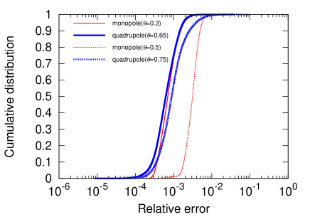
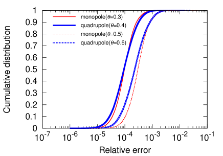
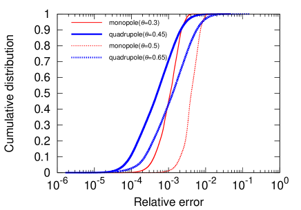
Figure 1: Cumulative distribution of errors in forces of particles with $N=65,536$. From top to bottom, the particle distributions are a homogeneous sphere, a Plummer model and an exponential disk, respectively.

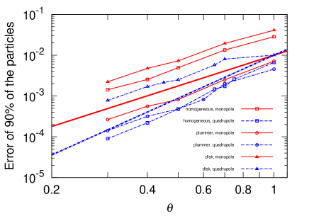
Figure 2: Error of 90% of the particles as a function of $\theta$. The squares, circles, and triangles show the result of a homogeneous sphere, a Plummer model, and a disk, respectively. The solid and dashed lines without points show $\theta^{5/2}$ and $\theta^{7/2}$ scaling, respectively.

5 Performance

In this section, we compare the performance of our implementation, original Phantom-GRAPE, and the pseudoparticle multipole method when the same force accuracy is imposed. The system we used to measure the performance is shown in Table 2. We used only one core, and Intel Turbo Boost Technology is enabled. Compiler options were -O3 -ffast-math -funroll-loops. Theoretical peak FLOPS of the system per core is 67.2 GFLOPS. The values of $\theta$ when we utilize quadrupole moments are based on the result that we described in section 4.

Table 2: The system we use to measure the performance.

CPU	Intel Xeon E5-2683 v4 2.10GHz
Memory	128GB
OS	CentOS Linux release 7.3.1611 (core)
Compiler	gcc 4.8.5 20150623 (Red Hat 4.8.5-11)

5.1 Comparison of calculation time when the same accuracy is required

Table 5.1 shows the wall clock time for evaluating forces and potentials of all the particles with $N=4,194,304$. In general, when we utilize quadrupole moments, the time consumed in the tree construction becomes slightly longer because quadrupole tensors of cells are calculated. When we use the pseudoparticle multipole method, the time consumed in the tree construction becomes longer because of the positioning of pseudoparticles.

The simulations of the homogeneous sphere with only the monopole moments can be accelerated from 1.23 to 2.20 times faster when we use our code and evaluate quadrupole terms. The simulations of the exponential disk using only the monopole terms with $\theta=0.3$ can be accelerated 1.13 times faster when we use our implementation and set $\theta=0.45$. In other $\theta$ and particle distribution, using the quadrupole terms slows simulations. As described in section 4, using quadrupole terms allows us to use significantly larger $\theta$ than using only the monopole in a homogeneous system, while we can increase $\theta$ moderately in a clustered system. Therefore, more interactions from particles are approximated by quadrupole expansion in a homogeneous system than in a clustered system. Thus, using the quadrupole terms can efficiently accelerate simulations of a homogeneous system. In the clustered system such as the disk and the Plummer model, the number of approximated interactions by using quadrupole terms and larger $\theta$ is not enough to negate the increased calculation cost by computing quadrupole terms.

Our implementation is always faster than the combination of pseudoparticle multipole method and Phantom-GRAPE for collisionless simulations by a factor of 1.1 in any condition because calculations such as diagonalizations of quadrupole tensors are unnecessary.

cccccccc Wall clock time for evaluating forces and potentials of all the particles with $N=4,194,304$. “Monopole” calculates only monopole terms. “Pseudoparticle” calculates quadrupole terms with pseudoparticles. “Quadrupole” calculates quadrupole terms with our implementation. “Homogeneous” is the homogeneous sphere. “Plummer” is the Plummer model. “Disk” is the exponential disk. $T_{\mathrm{construct}}$, $T_{\mathrm{traverse}}$, and $T_{\mathrm{force}}$ are time for tree constructions, tree traverse, force calculation, respectively. $T_{\mathrm{total}}$ is total time. The column ”Ratio” is ratios of the total time to that of using only monopole. Program $\theta$ Particle distribution $T_{\mathrm{construct}}$[s] $T_{\mathrm{traverse}}$[s] $T_{\mathrm{force}}$[s] $T_{\mathrm{total}}$[s] Ratio
Program $\theta$ Particle distribution $T_{\mathrm{construct}}$[s] $T_{\mathrm{traverse}}$[s] $T_{\mathrm{force}}$[s] $T_{\mathrm{total}}$[s] Ratio
monopole 0.3 Homogeneous 1.06 3.03 19.82 23.99 1
pseudoparticle 0.65 Homogeneous 1.67 1.20 8.96 11.91 0.50
quadrupole 0.65 Homogeneous 1.10 1.16 8.53 10.88 0.45
monopole 0.5 Homogeneous 1.06 1.34 7.77 10.26 1
pseudoparticle 0.75 Homogeneous 1.67 0.94 6.53 9.22 0.90
quadrupole 0.75 Homogeneous 1.10 0.92 6.25 8.35 0.81
monopole 0.3 Plummer 2.05 7.79 31.30 41.23 1
pseudoparticle 0.4 Plummer 2.70 6.41 39.41 48.61 1.18
quadrupole 0.4 Plummer 2.11 5.81 36.64 44.65 1.08
monopole 0.5 Plummer 2.05 2.71 10.28 15.13 1
pseudoparticle 0.6 Plummer 2.69 3.22 18.31 24.30 1.61
quadrupole 0.6 Plummer 2.11 2.96 17.11 22.26 1.47
monopole 0.3 Disk 1.45 5.49 20.95 28.01 1
pseudoparticle 0.45 Disk 2.10 3.76 21.11 27.09 0.97
quadrupole 0.45 Disk 1.51 3.52 19.72 24.86 0.89
monopole 0.5 Disk 1.45 2.22 7.96 11.75 1
pseudoparticle 0.65 Disk 2.11 1.98 9.70 13.92 1.18
quadrupole 0.65 Disk 1.51 1.88 9.18 12.67 1.08

5.2 The dependency of calculation time in the number of particles and interactions per second

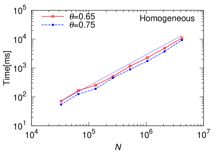
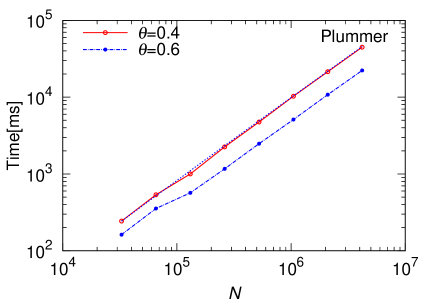
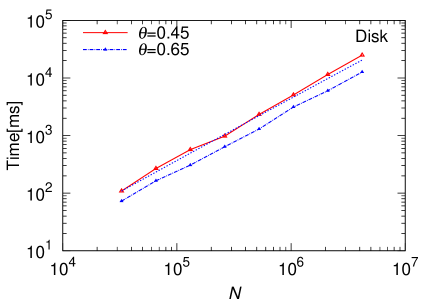
Figure 3: Wall clock time for calculating forces and potentials of all the particles. From top to bottom, the particle distributions are a homogeneous sphere, a Plummer model and an exponential disk, respectively. Dotted lines show $N\log N$ scaling.

Figure 3 shows wall clock time on various $N$ for calculating forces and potentials of particles in the homogeneous sphere (top), the Plummer model (middle), and the exponential disk (bottom), respectively. Solid curves are for small $\theta$, and dashed curves with points are for large $\theta$. Dashed lines without point show $N\log N$ scaling. We can see that the total time to calculate the force and potential of particles is roughly proportional to $N\log N$. However, from $N=65,536$ to $N=131,072$ on the homogeneous sphere, the actual scaling of the total time slightly deviates from the $N\log N$ scaling. From $N=65,536$ to $N=131,072$, the depth level of the tree traversals became deep because of the nature of the hierarchical oct-tree structure. Thus, more part of interactions is approximated with the multipole expansions. Therefore, the total number of particle-particle and particle-cells interactions and the total calculation time deviates slightly from the $N\log N$ scaling. Deviation from $N\log N$ scaling can also be seen on the Plummer model and the disk. However, the deviation is not as obvious as that on the homogeneous sphere. The calculation time can fluctuate by other running processes.

As seen in Figure 4, the number of interactions from cells per second is greatly reduced in $N<262,144$. This slowdown comes from the overhead of storing $i$-particles into the structure named Ipdata. Our code, as well as the original Phantom-GRAPE (Tanikawa et al. (2013)) stores four $i$-particles into Ipdata. Each time a calculation of the net force on four $i$-particles is done, next four $i$-particles are loaded into Ipdata. The number of interaction is proportional to $n_{i}\times n_{j}$, where $n_{i}$ is the number of $i$-particles, and the computational cost for storing $i$-particles is proportional to $n_{i}$. If $N$ becomes fewer, $n_{i}$ and $n_{j}$ also become fewer. Therefore, the overhead of storing $i$-particles becomes relatively large compared to the calculation of interactions itself, resulting in the speed down of the calculation of interactions. This behavior is also seen in the original Phantom-GRAPE (Tanikawa et al. (2013)), which shows lower performance for smaller $n_{i}$ and $n_{j}$.

Theoretical peak FLOPS per core of the CPU which we use is 67.2 GFLOPS, however, this value is based on the assumption that the CPU is executing FMA operations all the time. Actually, 36 counts of floating point operations in our code are FMA , and the rest come from non-FMA, add, subtract, multiply, and inverse-square root operations. Therefore, if we count 71 and 58 operations per interaction, theoretical peak FLOPS in our code with Intel Xeon E5-2683 v4 is 50.6 and 54.5 GFLOPS, respectively. From Figure 4, the numbers of interactions from cells per second are $\sim 7\times 10^{8}$ at sufficiently large $N$. For 71 and 58 operations per interaction, the measured performances of our code are 50 and 41 GFLOPS, which correspond to 99% and 75% of the peak.

To validate effectiveness of our implementation for astrophysical regimes, we performed three cold collapse simulations. We set the gravitational constant, the total mass of particles, the unit length, the total number of particles, the time step, and the softening length as $G=1$, $M=1$, $R=1$, $N=4,194,304$, $\Delta t=2^{-8}$, $\epsilon=2^{-8}$, respectively. The initial particle distribution was the homogeneous sphere whose radius is a unity, and the initial virial ratio was $0.1$. Three simulations were conducted on the machine shown in Table 2 with 30 CPU cores. Differences between the three simulations are $\theta$ and whether quadrupole terms are calculated. Simulation A utilized only monopole terms with $\theta=0.3$. Simulation B and C calculated quadrupole terms and used $\theta=0.4$ and 0.65. Figure 5 shows the radial density profiles of these simulations at $t=10$. Note that we plotted from $R=0.01$, which is about five times of $\epsilon=2^{-8}$. The results of the three simulations agree well each other.

The particle distribution is nearly homogeneous at $t<1$. Thus, if we consider accuracy only at $t<1$, we can use $\theta=0.65$ when we calculate quadrupole terms to achieve comparable accuracy with only monopole terms as shown in Figure 1. The collapse occurs around $t=1$, and then a dense flat core forms at $t>1$ as shown in Figure 5. Therefore, if we take account of accuracy at $t>1$, it is assumed that we should use $\theta=0.4$ rather than $\theta=0.65$ when quadrupole terms are adopted. However, there was little difference in the density profiles. Thus, practically, we might be able to use larger $\theta$ than expected to reduce the calculation cost. The average calculation time per step of these simulations were 3.20 seconds, 3.70 seconds, and 2.05 seconds, for simulation A, B, and C, respectively. Therefore, we can gain 1.56 times better performance by calculating quadrupole terms with $\theta=0.65$ than by calculating only monopole terms of $\theta=0.3$.

As another practical astrophysical test, we performed a suite of cosmological $N$-body simulations using the same initial condition. The initial condition consists of $128^{3}$ dark matter particles in a comoving box of 103 Mpc and the mass resolution is $2.07\times 10^{10}\,M_{\odot}$. We generated the initial condition at $z=33$ by a publicly available code, MUSIC (Hahn & Abel, 2011). Here, we aim to evaluate the performance of our implementation for the late phase of large scale structure formation. For this reason, we first simulated this initial condition down to $z=1$ by a TreePM code, GreeM (Ishiyama et al., 2009, 2012). Then we identified particles within a spherical region with a radius of 51 Mpc on the box center and added hubble velocities to these particles. We use these particles as the new initial condition of our cosmological test calculations.

We simulated the initial condition from $z=1$ to $z=0$ with three different settings in the same manner as the cold collapse simulations shown above, namely, simulation A2 which utilized only monopole terms with $\theta=0.3$, simulation B2 and C2 which calculated quadrupole terms with $\theta=0.4$ and $\theta=0.65$. We also conducted the full box simulation by the TreePM. Figure 6 shows the mass functions of dark matter halos at $z=0$, identified by ROCKSTAR phase space halo/subhalo finder (Behroozi et al., 2013). The results of the three tree simulations and TreePM simulation agree well each other and well fitted by a fitting function calibrated by a suite of huge simulations (Ishiyama et al., 2015).

In the late phase of large scale strcuture formation such as $z<1$, particle distributions are highly inhomogeneous because dense dark matter halos form everywhere, indicating that it should be more reasonable to use $\theta=0.4$ rather than $\theta=0.65$ when quadrupole terms are adopted as discussed in cold collapse simulations. However, the difference of halo mass functions is indistinguishable. Thus, practically, larger $\theta$ than expected might be allowed to reduce the calculation cost. The average calculation time per step of these simulations were 0.415 seconds, 0.441 seconds, and 0.292 seconds, for simulation A2, B2, and C2, respectively. Therefore, these results demonstrate that we can gain 1.42 times better performance by our implementation. These simple tests reinforce the effectiveness of our implementation for some astrophysical targets.

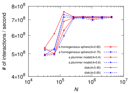
Figure 4: Numbers of interactions from cells per second. Note that particle-particle interactions are excluded. The squares, circles, and triangles show the result of a homogeneous sphere, a Plummer model, and a disk, respectively. Solid curves show the result for smaller $\theta$. Dotted curves show the result for larger $\theta$.

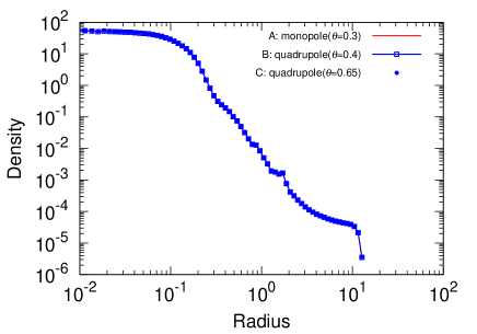
Figure 5: Radial density profiles of cold collapse simulations at $t=10$. Solid curves without points and with open squares show the results of simulations that utilized only monopole terms with $\theta=0.3$ (simulation A) and up to quadrupole terms with $\theta=0.4$ (simulation B), respectively. Circles show the result of simulation that utilized up to quadrupole terms with $\theta=0.65$ (simulation C).

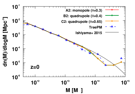
Figure 6: Mass functions of dark matter halos at $z=0$ obtained in a suite of cosmological test simulations. Three solid curves with symbols are results from our implementation for three different settings. Dashed curve is obtained from the simulation done by the TreePM method (Ishiyama et al., 2009, 2012). Solid curve without symbols denotes a fitting function proposed by Ishiyama et al. (2015).

6 Discussion

In this section, we estimate the performance of our implementation on AVX-512 environment. In AVX-512, the number of SIMD registers is 32, which is twice of AVX2. This number is enough to hold data that are currently needed to load every time the force calculation loop is done. Line 18 to 23 in List 2 are the operations for loading coordinates of $i$-particles. Line 36 and 37 is the operation for loading the gravitational softening length. Line 98 and 107 are the operations for loading constant floating-point numbers, which are necessary to calculate the quadrupole term of equation (1) and the gravitational force given in equation (14), respectively. All data loaded by those operations do not change throughout the entire $j$ loop in the force calculation from Line 16 to 123 in List 2. Therefore, Line 18 to 23, Line 36, 37, 98, and 107 in List 2 can be moved to before the loop. Furthermore, the width of SIMD registers in AVX-512 is 512-bit, which is twice of AVX2. This enables us to remove Line 56 in List 2 because the elements of the quadrupole tensors of two $j$-cells, which are $6\times 2=12$ elements, can be stored in one register. Without additional instructions, we can replace six VSHUFPS operations from Line 57 to 62 in List 2 to six VPERMPS operations, which permute single-precision floating-point value. The detail of VPERMPS is available in IntelR 64 and IA-32 Architectures Software Developer’s Manual . Totally, we can reduce the numbers of operations in the force loop from 59 to 48. Furthermore, the AVX-512 instructions can simultaneously calculate 16 single-precision floating-point numbers because of the twice width of the SIMD registers. Overall, we can estimate that the calculation of quadrupole terms becomes $59/48\times 2=2.46$ times faster in AVX-512 than AVX2. The calculation of monopole terms will be twice faster in AVX-512 than AVX2 because of the twice width of the SIMD registers. It is difficult to gain speed up in other parts such as the tree construction and the tree traversal because hierarchical oct-tree structures are used. Therefore, we assume that the calculation time for tree construction and tree traversal does not change on AVX-512 environment compared to that of AVX2 environment.

Table 6 is the estimated ratios of the time for calculating forces to that of using only the monopole on AVX-512 environment. Our implementation gives 1.08 times faster using the quadrupole terms with $\theta=0.4$ than using only monopole terms with $\theta=0.3$ for the Plummer model, and 1.02 times faster with $\theta=0.65$ than that of $\theta=0.5$ with using monopole terms only in the disk.

cccc Estimated ratios of the time for calculating forces and potentials to that of using only the monopole when we assume that the force calculation part is implemented with AVX-512. “Monopole” calculates only monopole terms. “Quadrupole” calculates quadrupole terms with our implementation. “Homogeneous” is the homogeneous sphere. “Plummer” is the Plummer model. “Disk” is the exponential disk. Program $\theta$ Particle distribution Ratio
Program $\theta$ Particle distribution Ratio
monopole 0.3 Homogeneous 1
quadrupole 0.65 Homogeneous 0.44
monopole 0.5 Homogeneous 1
quadrupole 0.75 Homogeneous 0.77
monopole 0.3 Plummer 1
quadrupole 0.4 Plummer 0.93
monopole 0.5 Plummer 1
quadrupole 0.6 Plummer 1.26
monopole 0.3 Disk 1
quadrupole 0.45 Disk 0.79
monopole 0.5 Disk 1
quadrupole 0.65 Disk 0.98

7 Summary

We have developed a highly-tuned software library to accelerate the calculations of quadrupole term with the AVX2 instructions on the basis of original Phantom-GRAPE (Tanikawa et al. (2013)). Our implementation allows simulating homogeneous systems such as the large-scale structure of the universe up to 2.2 times faster than that with only monopole terms. Also, our implementation shows 1.1 times higher performance than the combination of the pseudoparticle multipole method and Phantom-GRAPE. Further improvement of the performance is estimated when we implement our code with the new SIMD instruction set, AVX-512. On AVX-512 environment, our code is expected to be able to accelerate simulations of clustered system up to 1.08 times faster than that with only monopole terms. Our implementation will be more useful as the length of the SIMD registers gets longer. Our code in this work will be publicly available at the official website of Phantom-GRAPE .

We thank the anonymous referee for his/her valuable comments. We thank Kohji Yoshikawa, Ataru Tanikawa, and Takayuki Saitoh for fruitful discussions and comments. This work has been supported by MEXT as “Priority Issue on Post-K computer” (Elucidation of the Fundamental Laws and Evolution of the Universe) and JICFuS. We thank the support by MEXT/JSPS KAKENHI Grant Number 15H01030 and 17H04828. This work was supported by the Chiba University SEEDS Fund (Chiba University Open Recruitment for International Exchange Program).

References

- Bagla (2002) Bagla, J.S. 2002, J. Astorophys. Astron., 23, 185
- Barnes (1990) Barnes, J. 1990, Journal of Computational Physics, 87, 161
- Barnes & Hut (1986) Barnes, J., & Hut, P. 1986, Nature, 324, 446
- Barnes & Hut (1989) Barnes, J., & Hut, P. 1989, ApJS, 70, 389
- Bédorf et al. (2014) Bédorf, J., Gaburov, E., Fujii, M. S., Nitadori, K., Ishiyama, T., Portegies Zwart, S. 2014, SC ’14: Proceedings of the International Conference for High Performance Computing, Networking, Storage and Analysis, 54
- Bédorf et al. (2012) Bédorf, J., Gaburov, E., Portegies Zwart, S. 2012, Journal of Computational Physics, 231, 2825
- Behroozi et al. (2013) Behroozi, P. S., Wechsler, R. H., Wu, H. 2013, ApJ, 762, 109
- Dubinski et al. (2004) Dubinski, J., Kim, J., Park, C., Humble, R. 2004, New Astronomy, 9, 111
- Fukushige et al. (2005) Fukushige, T., Makino, J., Kawai, A. 2005, PASJ, 57, 1009
- Hahn & Abel (2011) Hahn, O., Abel, T. 2011, MNRAS, 415, 2101
- Hamada et al. (2009) Hamada, T., Narumi, T., Yokota, R., Yasuoka, K., Nitadori, K., Taiji, M. 2009, SC ’09 Proceedings of the Conference on High Performance Computing Networking, Storage and Analysis, 1
- Hamada & Nitadori (2010) Hamada, T., Nitadori, K. 2010, SC ’10: Proceedings of the 2010 ACM/IEEE International Conference for High Performance Computing, Networking, Storage and Analysis, 1
- Hernquist (1987) Hernquist, L. 1987, ApJS, 64, 715
- Hockney & Eastwood (1981) Hockney, R. W., & Eastwood, J. W. 1981, Computer Simulation Using Particles (New York: McGraw-Hill)
- Ishiyama et al. (2015) Ishiyama, T., Enoki, M., Kobayashi, M. A. R., Makiya, R., Nagashima, M., Oogi, T. 2015, PASJ, 67, 61
- Ishiyama et al. (2009) Ishiyama, T., Fukushige, T., Makino, J. 2009, PASJ, 61, 1319
- Ishiyama et al. (2012) Ishiyama, T., Nitadori, K., Makino, J. 2012, SC ’12 Proceedings of the International Conference on High Performance Computing, Networking, Storage and Analysis, 5, 1
- Kawai et al. (2000) Kawai, A., Fukushige, T., Makino, J., Taiji, M. 2000, PASJ, 52, 659
- Kawai & Makino (2001) Kawai, A., & Makino, J. 2001, ApJ, 550, 143
- Makino (1990) Makino, J. 1990, Journal of Computational Physics, 88, 393
- Makino (2004) Makino, J. 2004, PASJ, 56, 521
- Makino & Aarseth (1992) Makino, J., & Aarseth, S. J. 1992, PASJ, 44, 141
- Makino et al. (2003) Makino, J., Fukushige, T., Koga, M., Namura, K. 2003, PASJ, 55, 1163
- Miki et al. (2012) Miki, Y., Takahashi, D., Mori, M. 2012, Procedia Computer Science, 9, 96
- Nakasato (2012) Nakasato, N. 2012, Journal of Computational Science, 3, 132
- Nitadori et al. (2006) Nitadori, K., Makino, J., Hut, P. 2006, New Astronomy, 12, 169
- Oshino et al. (2011) Oshino, S., Funato, Y., Makino, J. 2011, PASJ, 63, 881
- Springel (2005) Springel, V. 2005, MNRAS, 364, 1105
- Sugimoto et al. (1990) Sugimoto, D., Chikada, Y., Makino, J., Ito, T., Ebisuzaki, T., Umemura, M. 1990, Nature, 345, 33
- Tanikawa et al. (2013) Tanikawa, A., Yoshikawa, K., Nitadori, K., Okamoto, T. 2013, New Astronomy, 19, 74
- Tanikawa et al. (2012) Tanikawa, A., Yoshikawa, K., Okamoto, T., Nitadori, K. 2012, New Astronomy, 17, 82
- Wang et al. (2018) Wang, Q., Cao, Z., Gao, L., Chi, X., Meng, C., Wang, J., Wang, L. 2018, Res. Astron. Astrophys, 18, 6
- Xu (1995) Xu, G. 1995, ApJS, 98, 355
- Yoshikawa & Fukushige (2005) Yoshikawa, K., & Fukushige, T. 2005, PASJ, 57, 849