Beyond Roll-Up’s and Drill-Down’s: An Intentional Analytics Model to Reinvent OLAP (long-version)

Abstract

This paper structures a novel vision for OLAP by fundamentally redefining several of the pillars on which OLAP has been based for the last 20 years. We redefine OLAP queries, in order to move to higher degrees of abstraction from roll-up’s and drill-down’s, and we propose a set of novel intentional OLAP operators, namely, describe, assess, explain, predict, and suggest, which express the user’s need for results. We fundamentally redefine what a query answer is, and escape from the constraint that the answer is a set of tuples; on the contrary, we complement the set of tuples with models (typically, but not exclusively, results of data mining algorithms over the involved data) that concisely represent the internal structure or correlations of the data. Due to the diverse nature of the involved models, we come up (for the first time ever, to the best of our knowledge) with a unifying framework for them, that places its pillars on the extension of each data cell of a cube with information about the models that pertain to it – practically converting the small parts that build up the models to data that annotate each cell. We exploit this data-to-model mapping to provide highlights of the data, by isolating data and models that maximize the delivery of new information to the user. We introduce a novel method for assessing the surprise that a new query result brings to the user, with respect to the information contained in previous results the user has seen via a new interestingness measure. The individual parts of our proposal are integrated in a new data model for OLAP, which we call the Intentional Analytics Model. We complement our contribution with a list of significant open problems for the community to address.

1 Introduction and overview

How will business intelligence (BI) look like 10 years from now? What foundations should academia build in order to rigorously support the building of tools, the optimization of OLAP sessions, and the training of data scientists around a logical paradigm? In this paper, we revisit the foundations of OLAP in an attempt to address the aforementioned questions.

To start with, it is worth to shortly revisit the evolution of analytical querying so far.

• At the beginning of time, people would be working with relational queries and recordsets returned by these queries. This treatment of BI was very DBMS-oriented, as the focus of attention was on what the DBMS can do for the users [1].

• Then, both the scientific community and the industry understood that it is possible to simplify the life of the business users, by providing a simpler view of the data to them, and hiding the complexities of the underlying database. So, users would deal (on-line) with cubes, rather than with traditional database data, which gives a very elegant simplification of the data to the user, as all the joins and aggregations are taken care by the system. The operators would be cube-oriented, one level of abstraction above the database operators and would involve so-called OLAP operators such as roll-ups, drill-downs, etc. (see for example [2]).

• Rapidly, apart from simply querying data, efforts focused on facilitating easier ways to navigate the multidimensional data space. Research proposed advanced operators permitting discovery-driven analysis via combinations of OLAP primitives [3, 4, 5]. More recently, different strategies in database exploration have been proposed as well, like keyword search over databases, presenting example tuples to infer the query, etc.

BI is now becoming more and more pervasive, which entails an increasing participation in the decision-making process of users with competence in the business domain but low ICT skills. This requires further investigation to provide users with even more effective and user-centered paradigms for analytical querying. As a further step in this direction, in this work we envision a new data model for OLAP, called Intentional Analytics Model. Here, data are accompanied by knowledge insights and both of them are considered as first class citizens of the data model. Indeed, the user explores the information space by submitting intentions of information goals, i.e., why she wants to discover relevant information rather than prescriptions of what data she needs, and receives both data and annotations of highly interesting subsets of them as results. Under the hood, the intentions are mapped to traditional OLAP operations and knowledge discovery algorithms. In a sense, our data model can be seen as a particular case of database exploration that takes advantage of OLAP primitives and cubes to support higher-level data analysis.

1.1 The revolution of Intentional Analytics

In our Intentional Analytics Model we redefine what a query is, with respect to both what users ask the system, what the answer entails, and how this answer is computed:

• What a query is. We start by redefining what a query is, by replacing the traditional query definition of which data are needed with a specification of why we need to explore the data space, so that query formulation is performed in a way that is closer to the users’ analytical goals. Specifically, we propose to replace traditional OLAP operators with intentional operators; this means that, instead of operating with cubes in terms of roll-ups and drill-downs, users will state their analytical goals over the cubes as intentions. For example, instead of saying “drill down to store city” or “roll-up to product category”, the user might ask “explain the drop in the sales of this product family” or ”assess whether the sales in a particular region are abnormal or not”.

• What the answer to a query is. We argue we can no longer remain with plain cubes as the answers to queries. If we want to replace simple query answering with insight gaining, the answer to a query cannot be just data – even if they are nicely packaged via fancy visualizations of textual storytelling. We believe that the answer to an intentional query is a dashboard, including (a) one or more cubes with the appropriate visualization and data narrations, (b) concise representations of knowledge hidden in the data, possibly obtained through automated mining of models and patterns (e.g., via decision trees or regressions) and (c) highlights, i.e., significant “jewels” hidden in the result that highlight parts of the data and model spaces that give significant insights to the user’s intention.

• Highlight mining. Assuming that each intentional operation is accompanied by a set of knowledge extraction algorithms like outlier detection, regressions, correlations of measures and attributes, decision trees and other similar operations, one particular aspect of profound importance is how do we decide which of the models produced and which subset of the data and model space in particular is really standing out as a highlight. To assess the importance of findings, we assess them in terms of their significance, using a subjective interestingness measure which follows the framework of [7] for pattern exploration.

1.2 The vision in a nutshell

We assume a typical OLAP setting [8] defined on a multidimensional space with cubes holding the information for analysts and dimensions providing a context for facts. This is especially important if combined with the fact that dimension values come in hierarchies of levels; therefore, every single fact can be simultaneously placed in multiple hierarchically structured contexts, providing thus the ability to analyze sets of facts from multiple perspectives. The underlying data sets include measures that are characterized with respect to these dimensions. Cube queries involve measure aggregations at specific levels of granularity per dimension, along with filtering of data for specific values of interest. For a formal treatment of the data model of our approach, one can refer to Appendix of this paper (practically extending the data model of [9]).

In our vision, an OLAP session is a sequence of dashboards that the analyst sees, each with its own information, including data, charts and informative summaries of KPI performance. The sequence is produced by the actions of the analyst that changes the contents of the dashboard by requesting more information on the basis of a set of operations made available to him by the tool.

The main idea behind the transitions between the states of session, which is obtained via the user operations, is that we move from a concrete data model of logical operators like roll-up’s and drill down’s, to an intentional data model where the user expresses, in terms of operators, high-level requirements like ”explain a certain phenomenon”, ”predict the future values” and these high-level requirements have to be automatically translated to specific OLAP and Data Mining algorithms that will carry the answer. This can also facilitate greatly the extraction of highlights, as the user’s goal is explicitly stated to the system.

Intentional operators. In contrast to other data models where a user operation would practically be a query (relational or multidimensional), in our data model, a user operation characterizes the intention of the user with respect to her information need.

Example 1

Observe the cube depicted in Table 1. This is a cube computed over a detailed data set on working hours and depicts the weekly working hours of people that (a) work with pay and (b) have completed a post-secondary education, grouped by their education level and work class. The columns of the result pertain to the values of the dimension education that demonstrated at the top row, and the rows pertain to the values of the dimension work class that are demonstrated at the leftmost columns.

Weekly Hrs	Assoc	Post-grad	Some-college	University
Gov	40.73	43.58	38.38	42.14
Private	41.06	45.19	38.73	43.06
Self-emp	46.68	47.24	45.7	46.61

Table 1: Example of a cube $C^{O}$ that serves as the starting point of a user operation

The user studies this cube in a dashboard and has several opportunities to ask a subsequent query. We list the options that our data model equips the user with:

• A first remark the user makes can be that the observed table presents information in adequate detail with respect to the education categories but fails to Describe in adequate detail the information with respect to the work class. Changing the level of detail or the focus of the presented information answers the question ”Give me a different description of what the data tell us!”.

• A second possible exploration concerns the answer to the question posed to the system ”Now that I know the situation, can you Assess how good the situation is compared to a reference benchmark?”. For example, the analyst might want to know how is the current status assessed when compared to the previous 10 years, or compared to ”similar” countries, or equally interesting, how is the situation assessed when compared to the goals that the state has put with respect to the working hours of people.

• ”Why is the situation as it is now?” Can you Explain why things are in the current status? Is the number of working hours correlated to the educational level (observe the monotonicity with respect to the work class – each row is increasing compared to its rows above it)? Or maybe it is correlated to a hidden variable?

• ”Henceforth how will the situation be?” Can you Predict how things will be in the near future? Are there regression or timeseries analysis models that can be employed to tell us what the future status will be, based on the current data?

Dashboards as answers to queries. The states of a session are dashboards. In the current state of practice, a dashboard is a pre-designed collection of charts and performance summaries, based on the results of several OLAP queries that are executed over the underlying data. The novelty of our proposal is founded on the idea that a dashboard, being the result of a user operation, includes (a) the data that answer the queries of a dashboard, (b) models that are concise representations of knowledge about these data, either extracted via machine learning algorithms or infused by the analyst in the form of KPI’s, measure correlations or rules, and (c) highlights, which are important subsets of the knowledge and data artifacts that particularly address the user’s intention. The entire result is appropriately visualized and accompanied by textual descriptions (see [9] for a larger discussion on data narration). Therefore the dashboard, which is the ultimate answer to a user operation, replaces query answering by insight gaining, via the appropriate enrichment of query results with knowledge, annotations of importance and appropriate packaging. In order to construct a dashboard, we envision several computations taking place. Here is the sequence of the performed actions:

1. First, the queries of the state’s dashboard are issued and their results, the generating data of the dashboard, are computed. Any straightforward computations for extra, derived columns of the dashboard (e.g., $gain=price-cost$) are performed too.

2. Then, the available data are fed to model-extraction algorithms for the computation of models that abstract, summarize and provide patterns and insights for the data.

3. The potentially large amount of data and models computed has to be ranked and assessed on their interestingness for the analyst; the most important findings are classified as the dashboards highlights to be used for providing the main insights and the main directions for future transitions by the analyst.

4. The above are accompanied by visualization, text construction and reporting tasks that aim the process of understanding and communicating the main findings.

Models in a dashboard. Whereas speedometers and charts are the current state of practice in the area of BI, our vision extends beyond that. The automatic assessment and critical characterization of the presented data will be part of the BI of the near-future. See some simple cases based on the example of observing sales data of an international company:

• Sales data will be automatically characterized with respect to a decision tree that classifies them (e.g., as ”successful”, ”risky”, ”potentially hazardous” etc).

• Sales per country will be automatically clustered to reveal similarities and differences, as a first step towards understanding outliers and non-expected behavior.

• Aggregate sales over significant periods will be fed into time series analysis and forecasting methods to automatically detect trends, seasonalities and to deduce future values.

We consider the plugging of data analysis algorithms in the back-stage of a dashboard as an indispensable part of BI. These algorithms can range from very simple ones (e.g., finding the top values of a cuboid, or detecting whether a dimension value is systematically related to top or bottom sales) to very complicated ones (like, for example, outlier detection, dimensionality reduction, etc). Most importantly, as the operation of the algorithms will likely be as transparent as possible to the end user, their execution will require an almost automatic tuning of their parameters. The findings of these algorithms will be models of the data that are typically (not always) used to annotate the existing data with characterizations and offer focus points to the visualization of the dashboard (forecasts, outliers, dimension values that dominate top or bottom measures, $\ldots$). The models themselves give a multitude of results. However, some of these results indicate that a part of a dashboard’s data are of important interestingness value to the end user. Due to that, we collectively refer to the important results of the execution of these algorithms as highlights, in an attempt to show that the aim is to enrich the current data-intensive dashboards with knowledge that is worth exploring or using for decision making.

Example 2

Assume now that the Ministry of Labor, based on the data of a previous census, has set-up some goals for the improvement of labor. Assume also that per combination of education type and workplace, a specific goal, say $Weekly~{}Working~{}Target$, has been assigned, saying that if the average number of weekly hours at work is in the area of [40-55] for any category, then this is $Expected$ behavior, whereas any other amount outside this domain is either $Low$, or $Excessive$. This is exactly what business analysts call a Key Performance Indicator (KPI)

Then, assume that the analyst of the Ministry wishes to evaluate the situation based on these goals, and in fact, in more details than the aggregate summary of Example 1. The analyst issues the composition of two commands:

Describe the data of $C^{O}$ in more details by workplace;
Assess Hours Per Week using Weekly Working Target.

The results are then depicted in the cube $C^{N}$ of Table 2. The system has automatically performed the following actions for the analyst:

• First, the necessary data are retrieved from the underlying database and the new cube, say $C^{N}$ is computed. This is practically a drill-down, in traditional OLAP terminology. The data are depicted in the first three columns of Table 2 (intentionally in non-pivot form for reasons to be made obvious right away).

• Second, the KPI, which is a very illustrative example of a model, assesses the data by labeling them according to the measure values of the new cube $C^{N}$ (column ”Assessment”). Observe that every cell of the cube is mapped to the respective value of the model!

• Finally, in an effort to discover interesting part of the new cube, an interestingness assessment is performed, in an attempt to answer the question: ”what is really surprising for the user?” To this end, a simple discrepancy model is used to split data based on the label assigned, as illustrated by the two antagonistic components displayed in the right-most part of Table 2. The highlight selection algorithm of the system selects the first of the two right-most columns, thus marking the cells with assessment $Low$ as the most interesting.

				Assessment		Discrepancy		Discrepancy
Assoc	Federal-gov	41.15		Expected		0		1
	Local-gov	41.33		Expected		0		1
	State-gov	39.09		Low		1		0
	Private	41.06		Expected		0		1
	Self-emp-inc	48.68		Expected		0		1
	Self-emp-not-inc	45.88		Expected		0		1
Post-grad	Federal-gov	43.86		Expected		0		1
	Local-gov	43.96		Expected		0		1
	State-gov	42.96		Expected		0		1
	Private	45.19		Expected		0		1
	Self-emp-inc	53.05		Expected		0		1
	Self-emp-not-inc	43.39		Expected		0		1
Some-college	Federal-gov	40.31		Expected		0		1
	Local-gov	40.14		Expected		0		1
	State-gov	34.73		Low		1		0
	Private	38.73		Low		1		0
	Self-emp-inc	49.31		Expected		0		1
	Self-emp-not-inc	44.03		Expected		0		1
University	Federal-gov	43.38		Expected		0		1
	Local-gov	42.34		Expected		0		1
	State-gov	40.82		Expected		0		1
	Private	43.06		Expected		0		1
	Self-emp-inc	49.91		Expected		0		1
	Self-emp-not-inc	44.44		Expected		0		1

Table 2: Assessment with KPI

1.3 Contribution and outline

The main contribution of this paper is that it structures a vision for the BI of the near future in terms of a data model, the Intentional Analytics Model, with novel concepts and operators. We aim our definitions to be broad enough, yet as precise as possible; at the same time, we want to link them as much as possible to the intentional nature of the next generation of BI tools, where the end-user requests information at a very high level and the system transforms these requests to concrete execution of algorithms in order to compute, visualize and comment data and important highlights among them as an answer to the information request made by the end-user.

1. We redefine what an OLAP query is and place particular emphasis to the introduction of high-level intentions as the pillar of querying. We propose several intentional operators addressing fundamental informational needs, like describe, assess, explain, predict and suggest to replace the existing data-centric state of the art operators like roll-up and drill down.

2. We redefine what a query answer is and we complement data with models to produce, along with visualizations and textual commentaries (not covered in this paper), dashboards as answers to user queries.

3. As part of this fundamental change of what a query answer is, we address the problem of integrating an extensible, heterogeneous sets of information models (ranging from simple correlations, to clusters and decision trees) in a uniform framework. Similarly to prediction cubes [10], this is achieved by extending each cell of a cube with both data and model information that pertain to it – practically converting information on models (the members of each cluster, the paths of a decision tree, the expected values of a regression formula) to data that annotate each cell. This data-to-model mapping is proved very powerful in that it allows the information of models to be treated as part of each cell, independently of the model type that generated it.

4. We facilitate the comparison of alternative models in terms of their interestingness via this integrated framework. We propose a simple method for assessing the significance of each model –practically, the surprise it brings to the user– that is built upon the data-to-model mapping. Hence, we are able to compute highlights, independently of the model types used.

Outline. The paper is structured as follows. In Section 2 we present background OLAP concepts and cube queries and we complement them with fundamental concepts of our method, specifically, models and highlights. In Section 3, we present our method for interestingness assessment and highlight selection. We present the intentional operators in Section 4. Related work is surveyed in Section 6. We conclude with open roads for future work in Section 7.

2 Data, Models, Model Components, Highlights and Dashboards

In this Section, we detail the fundamental concepts behind our proposal. We believe that the traditional understanding of the multidimensional data model is not adequate any more, and the emphasis of this paper is on its extension with models, highlights and intentional operators; therefore, we confine ourselves to presenting a simplified version of the data model in this section, and refer the interested reader to the Appendix for its thorough formal definition.

In our approach, each state of an OLAP session in the Intentional Analytics Model is a dashboard the user sees. A dashboard is ultimately based on the generating data provided by a finite collection of intentional queries, posed to the underlying database. However, a sharp distinction from previous approaches is that we do not restrict ourselves to data but enrich them with a set of interesting findings, which come in terms of models, i.e., results of data mining or machine learning algorithms applied over the data of a dashboard, and significant annotations of data with reference to the components of these models, to which we refer as highlights.

2.1 Data, cubes and cube queries

In this subsection we provide a concise formal background for modeling hierarchies, cubes, and queries.

The following list provides a fundamental terminology for the subsequent discussions

• We assume an environment structured as a multidimensional space. We assume that dimensions provide a context for facts [8]. A dimension is practically the active domain of attributes for facts, that is internally hierarchically structured.

• Each dimension comes with a hierarchy of levels. Each dimension (e.g., $StoreGeography$ or $SalesDate$)is a lattice of levels (e.g., $City$, $Prefecture$, $Country$, or $Day$, $Week$, $Month$, $Year$). Each level comes with an active domain of values and there are hierarchical mappings between values (e.g., the ancestor of city Paris at the country level is France). Domains have identifier attributes as well as other properties (e.g., a city can have population, surface, geolocation, etc). Being lattices, all hierarchies start with a common, lowest possible level of coarseness and, all its paths end up at a common highest level of coarseness (holding a single value, all).

• Facts are structured in cubes. A cube is defined with respect to several dimensions, fixed at specific levels and also includes a number of measures to hold the measurable aspects of its facts. Each record of a cube, also known as cell is a point in the multidimensional space of the cube’s dimensions hosting a set of measures. A detailed cube is a cube having all its dimensions fixed at the lowest possible level. Cubes may also be enriched via derived measures, computed by applying functions (e.g., $profit$ is a derived measure computed as $price*qty-cost$).

• A subcube is a subset of a cube derived by selecting a set of cells from a cube via a selection filter.

• A cube query is a cube too, specified by (a) the detailed cube over which it is imposed, (b) a selection condition that isolates the facts that qualify for further processing, (c) the grouping levels, which determine the coarseness of the result, and (d) an aggregation over some or all measures of the cube that accompanies the grouping levels in the final result.

Example 3

Consider the detailed cube for the well known Adult (a.k.a census income) dataset referring to data from 1994 USA census. There are 8 dimensions (Age, Native Country, Education, Occupation, Marital status, Work class, Race and Gender) in the data set and a single measure, Hours per Week. Each dimension comes with a lowest possible level, which we denote as $L_{0}$. This detailed data set will be the basis of our running example. Formally this detailed cube is a function $DS$: Dom($Age.L_{0})\times\ldots\times Dom(Gender.L_{0})\rightarrow Dom(Hours~{}per~{}Week)$, of schema $\langle\{$Age,…,Gender$\},\{$Hours per Week$\}\rangle$.

Example 4

The following cube query produces the cube of Table 16:

$C^{N}=\langle DS,$

Education.L3=’Post-secondary’ and Work_class.L2=’With-Pay’,

$\langle$ALL,ALL,L2,ALL,L0,ALL,ALL$\rangle,$

$Avg(Hours~{}per~{}Week)\rangle$

where the selection condition fixes Education to ’Post- Secondary’ (at level L3), and Work to ’With-Pay’ (at level L2), data is grouped by Education at level 2, and Work at level 0, and the Avg of Hours per Week is requested.

Weekly Hrs	Assoc	Post-grad	Some-college	University
Federal-gov	41.15	43.86	40.31	43.38
Local-gov	41.33	43.96	40.14	42.34
State-gov	39.09	42.96	34.73	40.82
Private	41.06	45.19	38.73	43.06
Self-emp-inc	48.68	53.05	49.31	49.91
Self-emp-not-inc	45.88	43.39	44.03	44.44

Table 3: A new cube $C^{N}$ as the output of the cube query of Example 14

For the reader familiar with OLAP terminology, the new cube $C^{N}$ resulting from the query, is practically the result of a Drill-Down operation over the old cube $C^{O}$ of Example 1.

2.2 Models

Models are concise, information-rich knowledge artifacts [11] that allow users to

• compute or predict values for measures that widen the users’ view on the situation presented by the observed data;

• document a-priori known, or discovered relationships hiding in the data;

• annotate data with respect to their status, based on a labeling scheme.

The space of possible models is vast as they range from simple functions (e.g., grossSales = qty * price) and measure correlations (e.g., the application of Kendal correlation to the pair [avgDailyTemperature, amtIceCreamSold]) to more elaborate schemes such as decision trees, clustering, etc.

2.2.1 Model Types

To create models we rely on an extensible palette of model types. Model types are molds for individual models. Essentially, model types are meta-concepts, used in the same fashion as data types are used for models of attributes in the relational data model, or complex types for object-valued attributes in the object-relational data model. Following the traditional terminology, the models that abide by the mold of a model type are called its ’instances’.

Definition 1 (Model Type)

A model type is defined by (i) a name, (ii) a signature for its input, including (ii’) a complex-type attribute model parameters with model-dependent parameters, (iii) a signature for its output, as a list of model components (to be defined next) including (iii’) a complex-type attribute model characterization with statistical characteristics of the entire model.

The semantics of a model type is not formally represented but rather intuitively implied by its name; this also implies the algorithm to be executed for the computation of models. The term “signature” implies a structuring in a list of named attributes (if needed, of complex type).

Observe that the definition, apart from structuring the input and the output takes into consideration two important aspects. Concerning the input, we want the input signature to host (a) the attributes and parameters that participate in the feeding of the algorithm’s execution (e.g., the algorithm and the distance used for clustering) as well as (b) the binding choices that we make (e.g., how many values we want for a top-k selection). Concerning the output, apart from providing a structure (see model components in the sequel), we also want to measure characteristics of the output, as for example, objective quality measures like ARI for clustering, ROC for prediction, etc.

2.2.2 Models: roles, taxonomy, usage

Models as instantiations of model types. A model is determined by applying a model type to a cube. This requires binding the attributes in the input and output signatures to specific levels and/or measures in the cube schema. For instance, a decision tree that receives a generic set of attributes as input and relates them to a labeling attribute via an output tree structure is a model type; a decision tree on cube LastYearCustomerPurchases over [location, age, income] that characterizes each fact using a labeling attribute purchaseHeight with values {low, med, high} is a model.

Definition 2 (Model)

A model is an instance of a model type, with (i) a binding to a cube $C$ over which it is imposed, (ii) a binding of the input signature of the model type to levels/measures of $C$ and constants (including binding the model parameters), (iii) the population of the output of the model type with model components, along with the computation of the model’s model characterization with statistical characteristics.

Example 5

Consider the cube $C^{N}$ of Example 14. Table 4 shows two models of two different model types over this cube. The first model is of type Rank and the second one is of type KPI. The input binding of the first model is $\langle$Hours per Week$\rangle$. The input binding of the second model is $\langle\{\langle[0,40),Low\rangle,\langle[40-55),Expected\rangle,\langle[55-],Excessive\rangle\},$Hours per Week$\rangle$. The population of the outputs of the two models correspond respectively to columns Rank and Assessment of the table.

		Weekly Hrs		Rank		Assessm.
Assoc	Federal-gov	41.15		17		Expected
	Local-gov	41.33		16		Expected
	State-gov	39.09		22		Low
	Private	41.06		18		Expected
	Self-emp-inc	48.68		4		Expected
	Self-emp-not-inc	45.88		5		Expected
Post-grad	Federal-gov	43.86		10		Expected
	Local-gov	43.96		9		Expected
	State-gov	42.96		14		Expected
	Private	45.19		6		Expected
	Self-emp-inc	53.05		1		Expected
	Self-emp-not-inc	43.39		11		Expected
Some-coll.	Federal-gov	40.31		20		Expected
	Local-gov	40.14		21		Expected
	State-gov	34.73		24		Low
	Private	38.73		23		Low
	Self-emp-inc	49.31		3		Expected
	Self-emp-not-inc	44.03		8		Expected
Univ.	Federal-gov	43.38		12		Expected
	Local-gov	42.34		15		Expected
	State-gov	40.82		19		Expected
	Private	43.06		13		Expected
	Self-emp-inc	49.91		2		Expected
	Self-emp-not-inc	44.44		7		Expected

Table 4: Two models over cube $C^{N}$

Role and purpose. A model is a concise representation of some knowledge about the data. This knowledge can be some relationship between data attributes, some property or characterization of subsets of data, or some computed value over the existing data. At the same time, despite its conciseness, typically a model also serves as an enrichment of the underlying data – in other words, each record of the data can be extended, annotated, or, in any case, enriched with extra information by the model.

A Taxonomy of models. In typical Machine Learning terminology, a model is a concise description of a data set that tries to “fit” the data in an accurate and semantically rich way; as such, it is driven by the data. Yet, some relevant and concise description of data (e.g., a formula on how measures interrelate, or some rule-based KPI) may as well be part of the domain knowledge the user has. Like in [12], we use the term model in both cases. So, in our approach models come in two flavors: (a) user-driven models, where it is the analyst who defines a model for the relationship/labeling of a set of attributes, based on her a-priori domain knowledge, and (b) data-driven models, where the analyst requests from the system to extract a model from a specified cube.

Regardless of flavors, a model enriches a cube in one or more of the following ways, to which we refer as intentions in this paper:

1. Description: the model describes the relationship between levels/measure of the cube(s), or between facts, or between existing and newly computed facts (e.g., customers are clustered according to their purchase frequency);

2. Assessment: the model characterizes each fact, or an entire cube, typically by comparing it to a baseline (e.g., the overall sales of TVs of this month are “disappointing” with reference to the average of last 3 years);

3. Explanation: the model gives an explanation for some relevant observation by concisely representing hidden relationships among the levels/measures of the cube(s) (e.g., the purchase amount of a customer is mainly determined by her age and income);

4. Prediction: the model forecasts cube facts (e.g., sales during next Christmas period are expected to be 10% higher than last year).

5. Suggestion: the model suggests the next query(s) in the analysis using a recommendation strategy (e.g., users who did a similar assessment of sales of TVs then saw sales of TVs in the neighboring countries).

In Figure 1, we concisely detail how alternative models (both user and data driven) are grouped for different intentions. For the sake of space, the figure does not include the two complex-type attributes that are present in all model types, namely: the complex-type model parameters attribute is omitted from the $Input$ signature column, and the complex-type model characterization attribute is omitted from the $Output$ signature column. The term Name Of Measure practically refers to the fact that models are applied over measures and thus, a parameter of which measure is going to be used for the application of the model is necessary.

Name	Input signature	Output signature
	Model types for description
Top-k	$\langle$Number Of Values,Name of Measure$\rangle$	$\langle$Rank$\rangle$
Outlier	$\langle$Threshold,Name of Measure$\rangle$	$\langle$Outlierness$\rangle$
Clustering	$\langle$Number Of Clusters,Name of Measure$\rangle$	$\langle$Cluster${}_{1},\ldots,$Cluster${}_{n},$Representative$\rangle$
Shrink	$\langle$Number Of Cells,Name of Measure$\rangle$	$\langle$Cell${}_{1},\ldots,$Cell${}_{n}\rangle$
Dominating Slice	$\langle$Name of Measure$\rangle$	$\langle$DomSlice${}_{1},\ldots,$DomSlice${}_{n}\rangle$
	Model types for assessment
KPI	$\langle\{$Labeling Rules$\},$Name of Measure$\rangle$	$\langle$Assessment$\rangle$
Function-based Benchmark	$\{function~{}parameters\}$	$\langle$Discrepancy$\rangle$
	Model types for explanation
Correlation	$\langle$Threshold,Name of Measure$\rangle$	$\langle$Participation$\rangle$
Regression	$\langle$Threshold,Name of Measure$\rangle$	$\langle$Discrepancy$\rangle$
Decision tree	$\langle\{\langle$Range,Label$\rangle\},\{\langle$Attributes$\rangle\},$Name of Measure$\rangle$	$\langle$Label$\rangle$
Statistical test	$\langle$Threshold,Name of Measure$\rangle$	$\langle$Discrepancy$\rangle$
	Model types for prediction
Auto-Regression	$\langle$Threshold,Name of Measure$\rangle$	$\langle$Discrepancy$\rangle$
Time Series Decomposition	$\langle\{$Thresholds$\},$Name of Measure$\rangle$	$\langle$Trend,Seasonality,Noise$\rangle$
	Model types for suggestion
Content-based	$\langle$Number Of Queries$\rangle$	$\langle$QueryID$\rangle$
Collaborative	$\langle$Number Of Queries$\rangle$	$\langle$QueryID$\rangle$
Hybrid	$\langle$Number Of Queries$\rangle$	$\langle$QueryID$\rangle$

Figure 1: A grouping of model types, organized per intention.

How to work with models. In terms of usage, the way of working with models is as follows:

1. Model construction or retrieval. Model construction is the step dedicated to taking the input data and extracting or assigning an abstraction of the relationships hidden in them. Be it the assignment of a function that computes a new measure, the choice of a time series analysis algorithm that splits a time series measure to 3 new measures (trend, periodicity, noise), or, the construction of a decision tree over the particular cube, the construction of a model is a representation of the relationships between the involved attributes.

2. Application of the model to the data. An extra step, which we introduce as a particularity of our method, is the linkage of the model to the data. Model application, is the step that computes, for each tuple of the input data, the output measures that the model type carries. Each input tuple is then practically extended with a set of output attributes pertaining to the model.

3. Highlight extraction. Highlight extraction is the step that focuses the interest of the user to a subset of the annotated data. By reusing the output of the model, highlight extraction algorithms can pick potential ”hidden jewels” or highlights out of the vastness of available data, and decide which of them are more significant for the user

Of course, the steps can be blended for optimization purposes; here we separate them to illustrate their role. In the subsequent subsections, we will elaborate more on the structure and role of the output of a model and its linkage to the data as well as on the issue of highlights. Before that, however, we would like to address the following important issue.

Can we automate parameter tuning and model invocation? Tuning the parameters for the invocation and application of a model type can range from one extreme, where everything is specified by the user, to the other extreme, where predefined values exist for every possible parameter. A middle-ground alternative is to consider a dynamic generation of models and tuning of parameters depending on the properties (size, content, etc.) of the cube the model is applied to. A statistical test can be used to decide whether a given model fits the data of the cube; for instance, the Hopkins statistics can be used to check for clustering tendency [13] and decide whether clustering is worth testing on the cube. We note that an entire field of research, called meta-learning, is devoted to answering problems like how to choose a learning algorithm based on data characteristics [14]. Practically, automated machine learning frameworks and tools (like e.g., auto-sklearn [15]) can be used to automatically select an algorithm and its parameters for a given dataset, given a computation cost.

2.2.3 Model Components

Model Components. The output of a model is of particular importance. The elements of the output of each model are called output model components. Specifically, we require that the output obeys a signature, meaning that the output is always structured as a list of attributes (it can be just one), each pertaining to a different component. Examples of output model components include:

• A time series splits each of its points to 3 measurements, specifically error, trend and seasonality (practically creating 3 times series in the place of one, whose sum reconstructs the original one).

• A clustering scheme includes a set of clusters, each coming with a centroid, as well as with an indication, for each tuple, of its participation to a specific cluster.

• A classification decision tree includes a tree structure, best expressed as the composition of a set of paths, leading to characterization classes; again, each class comprises a set of tuples in the underlying cube that pertain to it.

• An outlier includes an outlier strength measurement per cell.

• A top-k or a ranking components includes selecting the uppermost $k$ values and annotating the rest as of no interest, or, respectively, the ranking of all cells in terms of their measure value.

Data-to-model mappings. Is it possible to uniformly handle the heterogeneity of different model types? Clearly, a cluster is inherently different from a decision tree or the formula for a trend. Is there a unifying common ground to cover them all? The unifying essence of all the plethora of diverse model types is that all of them are annotations of the original data. At the end of the day, every component of a complex model type (be it a cluster id, a path in a decision tree and a resulting class, a characterization of the top-k tuples, or a trend formula): (a) refers to a subset of the input data and vice-versa, and, (b) refers to the overall model via a part-of relationship. So, once a model of the underlying data is available, our solution to the problem is to provide a distinct identity to the components of a complex model type (here: as a distinct attribute) and annotate or characterize the data with respect to the model component that pertains to them. In fact, this step can be blended within the model extraction itself. Examples of such annotations follow:

• Assuming a time series model that splits a time series to $trend$, $seasonality$ and $noise$, these attributes can be appended to the generating data set.

• Assuming a cluster model, the generating data can be annotated with the $id$ of the cluster to which they belong.

• Assuming a classification model, the input data can be labeled via an extra attribute with respect to the class(es) of the model to which they belong.

• Assuming a model of top-k values of a measure, the input data can be annotated with their rank, and whether they belong in the top-k set or not.

The above observations allow us to provide a data-to-model mapping. A notable property of our modeling is that we require model components to be directly mapped and linked to their generating data in a bidirectional mapping, so that the end-user can navigate back and forth between cube cells and their models.

Antagonism. In addition to the components in its output, it is possible that the binding of a model induces antagonistic components that provide an assignment of the cells of the cube to different components. Examples of antagonistic model components include:

• one component for each cluster of a clustering, to identify the participation of each cell to the cluster, and one component to identify the representative(s) of the cluster (e.g., medoid);

• one component for the outliers and one component for the non-outliers, based on a threshold on outlier strength measurement;

• one component for the top-k cells and one component for the non-top-k cells.

More frequently than not, this assignment to groups is a partition, i.e., each cell belongs to exactly one component. However, there are exceptions, like for example fuzzy clustering or fuzzy labeling. The ability to provide this assignment of cells to antagonistic components is fundamental to facilitate the highlight selection process. Take for example the case where we split the cells of the cube on the basis of a top-5 model (i.e., we set $Number~{}of~{}Values=5$ at the binding of the top-k model type) and we have two components, (a) one containing the top-5 cells, and, (b) another with the rest of the non-top-5 cells. The highlight selection process will then select which of these two components bears the greatest amount of new information to the user. Thus, the term antagonistic is justified, as the respective components antagonize to provide the maximum amount of surprise to the user. The antagonists can be either (a) components produced directly as the output of the model extraction algorithm, or (b) components derived from the regular output to serve the purpose of highlight extraction. As an example of the former case, consider any labeling algorithm (KPI, decision tree, or other), which by definition separates the cells into groups with the same label producing one component per label, so that these different components can antagonize with each other on which is the actual highlight. As an example of the latter case, consider the case of top-k cells, where the output component $Rank$ is used to derive two antagonists: Top-k and Non-Top-k.

Practically, we can define a model component as follows.

Definition 3 (Model Component)

A model component is a named attribute containing either the result of a model construction algorithm, or produced internally, as an induced attribute to be derived for highlight selection. The extent of a model component depends on the nature of the model. A model component can be annotated with its statistical characterizations via a component characterization attribute.

The statistical strength of each component (the number of cells being outliers, or the cohesion of a cluster) is different than the one of the entire model. Here, each component carries it own statistical characteristics.

Example 6

While Table 4 of Example 14 shows output components of two models over the cube $C^{N}$, Table 5 shows the facts of cube $C^{N}$ together with two antagonistic components of model Top-5, respectively attribute Top-5 and attribute Non-top-5, with their extents.

				Top-5		Non-top-5
Assoc	Federal-gov	41.15		0		1
	Local-gov	41.33		0		1
	State-gov	39.09		0		1
	Private	41.06		0		1
	Self-emp-inc	48.68		1		0
	Self-emp-not-inc	45.88		1		0
Post-grad	Federal-gov	43.86		0		1
	Local-gov	43.96		0		1
	State-gov	42.96		0		1
	Private	45.19		0		1
	Self-emp-inc	53.05		1		0
	Self-emp-not-inc	43.39		0		1
Some-college	Federal-gov	40.31		0		1
	Local-gov	40.14		0		1
	State-gov	34.73		0		1
	Private	38.73		0		1
	Self-emp-inc	49.31		1		0
	Self-emp-not-inc	44.03		0		1
Univesity	Federal-gov	43.38		0		1
	Local-gov	42.34		0		1
	State-gov	40.82		0		1
	Private	43.06		0		1
	Self-emp-inc	49.91		1		0
	Self-emp-not-inc	44.44		0		1

Table 5: Two antagonistic components of model type Top-k over cube $C^{N}$

The ability to annotate each cell of a cube with respect to a model component is of extreme importance and the driving force behind our definition, that practically models components as attributes of the relational data model. The possibility of integrating a vast space of heterogeneous models via a simple and uniform representation, which also facilitates a data-to-model mapping as suggested in [16], allows us to practically treat models as data too and use them for addressing the user’s information needs!

2.3 Highlights

As already mentioned, the set of highlights of the dashboard is a set of important findings that accompany the dashboard. These can be findings of any nature, e.g., important outliers in the contents of the dashboard’s data, all the tuples belonging to a certain class of a classification scheme, the top or bottom values of a measure, etc.

What is interesting for the user, however? Are there universal notions (esp., formulae) for interestingness [17]? Should we personalize interestingness for each user on the grounds of a profile? Maybe interestingness is defined by what everyone else found interesting? Or maybe interestingness is fundamentally dependent upon the combination of data and the original intention the user had when he queried the data? We are mainly driven by the last option, without, of course, disqualifying the others and in full comprehension that there is quite some research effort before crystallizing to a specific stance on the problem. Again, the holy grail here is to fully automate the proactive highlighting of data of interest for the user.

Whenever the result of a new user query is computed and new data, cuboids if you will, are acquired to answer the query, one or more models are automatically computed. The fundamental idea of our approach is that, ideally, one of the antagonistic components of one of these models is the most adequate to respond to the intention of the user. The determination of the quality that discriminates the most appropriate component, which we call interestingness, depends on several factors, including its relevance to the original intention, its novelty (to which extent it reveals new information that was previously unknown to the user) or its surprise (to which extent it contradicts previous beliefs of the user). For example, assume the user is assessing a measure (e.g., Sales) with respect to a benchmark (e.g., lastYearSales) and the model annotates each cell by its difference to the respective cell of the previous year and measures the $z~{}score$ of the difference over the population of differences. Then, the model can produce 3 components based on the ranges of $z~{}score$, e.g., (a) up to $\sigma$, (b) between $1\cdot\sigma$ and $2\cdot\sigma$, and (c) higher than $2\cdot\sigma$. The last component and the cells pertaining to it (those with $z~{}score$ higher than $2\cdot\sigma$) constitute the highlights of the operation.

The essence of highlight selection is therefore the identification of a specific model component that maximizes the interestingness of the information delivered to the user by it with respect to her original intention. The highlight is, then, the combination of the component and the data that refer to it.

The generalization of the above intuition to more sophisticated selection criteria is possible, of course. So, whereas here we select the top-1 component with respect to its interestingness, one can imagine schemes where the top-k are selected, or any component that surpasses an interestingness threshold. As already mentioned, the possibilities for defining highlight selection criteria are open and subject to lots of future work. In any case, we assume that we have (a) a scoring function $interestingness()$ that returns an interestingness score for each of the components of $M$, and, (b) a criterion $\phi_{H}$ to determine which component(s) qualify for highlights.

Another particular aspect that plugs into highlight selection is the idea of digging out the essence of a component. As every component annotates all the data of the input cube, assume now that we have a criterion for selecting its ”core data”. Assume that each model type has a selection criterion for the core data of its components, which we denote with $MC.coreElements$ that returns the set of elements that mostly pertain to the intuitive essence of a component, along with their respective cube cells, obtained via the 1:1 data-to-model mapping, which we denote $MC.coreCells$. To give a couple of concrete examples, here is a short list:

• Assume a clustering model with clusters being modeled as bitmaps, having 1 for the data that pertain to it and 0 for the rest. Then, the cells annotated with 1 comprise the essence of the component.

• Assume a decision tree, with classification paths being its components. Each path is also a bitmap of 1 and 0 depending on whether each cell pertains or not this path. The cells annotated with 1 in a path component are its essential, core cells.

• Alternatively, assume a classification scheme where the cube cells are assigned a particular label within a single-component model. Then, the core cells of the component are the ones that abide by the criterion used (”expected” values if the criterion is non-outlierness, ”low” or ”high” values if the criterion is outlierness.

So overall, depending on the model type $T$ that induces a structure for its output components and the criterion $\phi_{H}$, for each component we can compute a subset of the core elements, as well as the respective core cells that define the essence of the component. Notably, in the case where all components are bitmaps (which is always the case for a component with a discrete domain of values), the computation of the core elements and cells is independent of the criterion $\phi_{H}$.

Definition 4 (Highlight)

Given an intentional query $q$ issued over a cube $C^{O}$ of a dashboard, and resulting to a new cube $c$, a new model $M$ over cube $c$, with components $M.MC_{1},\ldots,M.MC_{k}$, a criterion for highlight selection $\phi_{H}$ (on the basis of a component scoring function $interestingness$), then, a highlight $h$ is a tuple including (a) $M.MC_{I}$, (b) the elements of $M.MC_{I}$ that are qualified as its core elements, and (c) the data of the new cube $C^{N}$ that pertain to it, via $MC_{I}.coreCells$, fulfilling the 1:1 mapping between (b) and (c) – i.e., a triplet $h$ = $\{MC_{I}$, $MC_{I}.coreElements$, $MC_{I}.coreCells\}$

In other words, there are many facets of a highlight: it is the most ”interesting” component, and, at the same time, the data that pertain to it.

2.4 Packaging it all in a dashboard, or, what the answer to a query really is

Having detailed models, model components and highlights, it is now time to integrate them into the big picture. We define dashboards as collections of cubes, coming along with their models and components. We refer to such a cube as an enhanced cube.

Definition 5 (Enhanced Cube)

The triple of a cube $C$, its (set of) models $\mathbf{M}$, and its highlights is called an enhanced cube.

Definition 6 (Dashboard)

A dashboard is a set of enhanced cubes.

A dashboard comes with visualizations, generation of textual commentaries and possibly automatic compilation of reports. We consider the inherent integration of these aspects into the overall framework as part of the future work and refer the interested reader to [18] for a first discussion and [9] for a review of related work.

3 Highlight Selection via a new Interestingness Measure

In this section, we present our approach for selecting significant highlights based on interestingness assessment. We start by motivating the subjective interestingness measure we adopt for significance. We then detail the highlight selection algorithm. Finally, we reuse our running example to conclude the section with a concrete case of highlight selection.

3.1 Interestingness measure

Exploratory Data Analysis (EDA) aims to provide insights to users by presenting them with human-digestible pieces of ”interesting” information about the data [19]. One particular EDA activity, Exploratory Data Mining (EDM), and mainly pattern-mining, has been particularly active in developing Interestingness Measures (IM) to filter the large set of artifacts resulting of the mining. In this context, interestingness has been quantified mainly in an objective way, in the sense that measures are agnostic of variations among users. Only recently has the concept of subjective interestingness been formalized, first as a quantification of unexpectedness relying on the concept of a belief system. This belief system formalizes the beliefs of the data miner, to which mining artifacts are contrasted to determine their interestingness [20]. In other words, the quantification of the subjective interestingness of an artifact is the result of its confrontation with a background model related to the user’s prior knowledge.

We believe that, in our context of user-centered analytical querying, interestingness must be defined subjectively, in the same vein as it is for EDM. However, to the best of our knowledge, no such concept of subjective interestingness exists in the general landscape of Interactive Database Exploration [21]. In this paper we introduce a completely novel scheme for interestingness assessment, which (a) exploits the fact that the user is involved in sessions of OLAP intentional queries (thus, previously seen results constitute prior beliefs) to offer the desired subjectivity, (b) since exploration takes place within a strictly structured information space (i.e., the multidimensional space defined by hierarchies), let us relate these previously seen cells to the new ones, and (c) quite importantly, takes the models derived into consideration, while at the same time staying model-independent. The core of our framework is the assessment of surprise, which is practically the difference of belief for the same subset of the multidimensional space, before and after an intentional query has been issued.

In our context, a user starts with a cube $C^{O}$, expresses an intention $q$ (e.g., Describe, Assess, etc.) that triggers the computation of new cube $C^{N}$, together with a set of $k$ models $M^{1},\ldots,M^{k}$, each of them with their components, $MC_{1}^{1},\ldots,MC_{m}^{k}$. Instead of interactively presenting one artifact extracted from the data chosen after its confrontation to prior knowledge, we are interested in presenting one of the antagonistic components among $MC_{1}^{1},\ldots,MC_{m}^{k}$, chosen as interesting after its confrontation with $C^{O}$. Therefore we measure surprise using an interestingness measure that quantifies for each antagonistic component the surprise brought by cube $C^{N}$ to cube $C^{0}$, as detailed next. The component with the highest surprise score is chosen to highlight the cells of $C^{N}$.

3.2 Principle of highlight selection

This generic principle of significance computation and highlight selection is depicted in Figure 2 and detailed in Algorithm 1. As displayed in Figure 2, this principle consists of the following steps. First, the intentional query is evaluated to get the new cube $C^{N}$ from $C^{O}$. Second, the models associated with the intention are instantiated and the components $MC_{1}^{1},\ldots,MC_{m}^{k}$ are obtained. Subsequently, a significance score is computed locally for each of the two cubes (step 3), and these scores are contrasted, resulting in a surprise score for each cell of $C^{N}$ (step 4). Then, each component among $MC_{1}^{1},\ldots,MC_{m}^{k}$ aggregates the surprise scores for the cells pertaining to it, resulting in a surprise score for this component (step 5). In a similar vein, we aggregate the component scores to compute surprise scores for entire models (Step 6). Finally, the component that maximizes the score is chosen for highlighting the cells of $C^{N}$ that pertain to it (step 7).

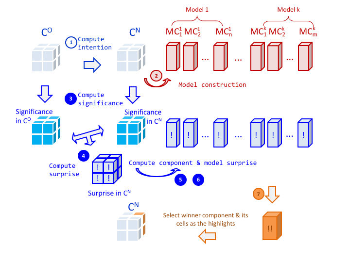
Figure 2: Principle of highlight selection

Data:

cube $C^{O}$

cube $C^{N}$

set of models $\{M^{1},\ldots,M^{k}\}$ with their components $MC_{1}^{1},\ldots,MC_{m}^{k}$

n:m relationship $proxies$ between the cells of $C^{O}$ and $C^{N}$

function $significance$ for computing the significance of a cell

function ${\cal D}$ for surprise characterization

function ${\cal A}^{C}$ for computing component scores

function ${\cal A}^{M}$ for computing model scores

Result:

a component among $MC_{1}^{1},\ldots,MC_{m}^{k}$

1 for all cells $c^{O}$ in $C^{O}$ do

2       compute $c^{O}.significance$

3for all cells $c^{N}$ in $C^{N}$ do

4       compute $c^{N}.significance$

5for all cells $c^{N}$ in $C^{N}$ do

6       compute $c^{N}.surprise={\cal D}(c^{N}.significance,c^{N}.proxies.significance)$

7for all components in $MC_{1}^{1},\ldots,MC_{m}^{k}$ do

8       compute $MC_{j}^{i}.surprise={\cal A}^{C}_{c^{N}\in MC_{j}^{i}}(c^{N}.surprise)$

9for all models in $M^{1},\ldots,M^{k}$ do

10      compute $M^{i}.surprise={\cal A}^{M}_{MC_{j}^{i}\in M^{i}}(MC_{j}^{i}.surprise)$

11return the component maximizing $MC_{j}^{i}.surprise$;

Algorithm 1 Highlight selection

Algorithm 1 describes the highlight selection procedure. The algorithm receives as input the two cubes $C^{O}$ and $C^{N}$, a set of model components $MC_{1}^{1}$, $\ldots$, $MC_{m}^{k}$ over $C^{N}$, and a set of functions depending on the intention. These functions include: (a) a relation $proxies$ that relate the cells of $C^{N}$ with the ones of $C^{O}$ (e.g., an ancestor relationship if the logical operation triggered by the intention is a drill-down), (b) a significance function for assessing how significant a cell is (note that this function may use one measure value or more), (c) a function $\cal{D}$ for computing the surprise between two significance scores, and (d) two functions ${\cal A}^{C}$ and ${\cal A}^{M}$ for aggregating surprise scores by model components and models, respectively. A few notes are due here:

• The relation $proxies$ is of $N$:$M$ nature to facilitate arbitrary relationships of old and new cells that can be produced via selections, roll-up’s, drill-down’s, or similar operations. In the typical scenario, the relationship will be annotated with a ’1’ in one of its two ends, facilitating easier computations of the subsequent steps.

• The $significance$ score is of great importance as it characterizes each cell with an objective importance (which is necessary in order to get the algorithm going). In our example that follows, significance is measured as outlierness, computed via a z-score; however, it is easy to conceive alternative objective significance scores, like, for example, the inverse (”typicality” if you will) to serve different intentions, the very same value of the measure, its rank, or others. Our framework is open-ended from this aspect for plugging more significance measures.

• The $surprise$ is the core of our method. Surprise exploits the fact that old and new cells are related via $proxies$, as they represent the same subspace of the entire multidimensional space. Thus, we can exploit this fact and contrast the prior and new belief (i.e., measure). For the rare case where the $proxies$ relationship is not straightforwardly defined for some cell, special care must be taken to contrast the cell’s significance to some representative significance value of the proxy cube (e.g., the mean or the average significance). Practically, this means that if there is no straightforward set of proxy cells (e.g., ancestor or descendants), we map the new cell to the entire previous cube. In the typical case, the ${\cal D}$ function can be a simple subtraction (as we envision it and use it here), or, again in an open-ended vein, another contrasting function (for example, one might consider the overall tendency of values in a subcube: if all values are increasing due to a trend, then the surprise s much less).

• The aggregation functions ${\cal A}^{C}$ and ${\cal A}^{M}$ can be any desirable aggregate function. In our example that follows we use the average value, however, sum, max, min, or other can be used too.

The algorithm unveils as follows. In lines 1-2 (respectively 3-4), a score is computed for each cell of $C^{O}$ (respectively $C^{N}$) using the $significance$ function. In lines 5-6, a surprise score is computed for each cell of $C^{N}$, by contrasting their significance score with the score(s) in their relatives in $C^{O}$. In line 7-8, a surprise score is computed for each components, by aggregating the surprise scores of the cells participating to the component. In line 9-10, a surprise score is computed for each models, by aggregating the surprise scores of the components of this model.

Before presenting a concrete example, we believe it is worth presenting a summary of the novelty and merits of our framework:

• We offer an interestingness framework that exploits the divine simplicity of the multidimensional data space of OLAP, as well as the existence of models along with the data – and it is thus, appropriate for the new model of OLAP that we propose.

• We escape the trap of objective, non-contextualized interestingness measures and provide a subjective measure, exploiting the transitions that OLAP queries via our operators offer, and based on the idea of prior belief (facts of the old cubes contrasted to the facts of new cubes). We base our approach to $surprise$ as the difference of belief for the same subset of the multidimensional space, obtained again by exploiting the relationship between old and new cells.

• We provide a method that exploits the data-to-model mappings of our model and is therefore independent of model types (which we deem as a major feature of the framework)

• We provide an open-ended framework where new definitions for objective significance, subjective surprise, delta, and aggregate functions are always possible.

Note that we provide a bottom-up method for computing highlights, starting from cells and ending up in models. The possibility of a top-down method, is of course, an open issue, but falls outside the scope of this paper.

Example 7

Recall cube $C^{O}$ of Example 1. Assume the user issues the intention with $C^{O}$ Describe Avg Working Hours by giving more details for workclass at the most detailed level. The first step in processing this intention results in evaluating the cube queries of Example 14 to drill-down to cube $C^{N}$, recalled below in Table 6.

The highlight selection algorithm is called with cubes $C^{O}$, $C^{N}$, a set of models and their model components and a set of functions. Regarding the models and model components, in this example, for the sake of brevity, we consider only two model components of two different models. They are displayed mapped on the cube $C^{N}$ in Table 6: (i) the top-5 cells (the 5 cells in yellow, note that this component is also presented in Example 6 in binary form) and (ii) the outliers greater than two standard deviation (the 2 cells in blue). The cell in green participates to both components. This example shows how the algorithm chooses among these two components.

The functions are as follows. The $proxies$ relationship allows to find in cube $C^{O}$ the ancestor of a cell of $C^{N}$. The $significance$ function used to compute the significance of each cell is the z-score, i.e., the number of standard deviations the value of this cell is from the mean of all the values of the aggregate cube. Function ${\cal D}$ is the difference and function ${\cal A}^{C}$ (respectively function ${\cal A}^{M}$) is the average.

$C^{N}$	Assoc	Post-grad	Some-coll.	Univ.
Federal-gov	41.15	43.86	40.31	43.38
Local-gov	41.33	43.96	40.14	42.34
State-gov	39.09	42.96	34.73	40.82
Private	41.06	45.19	38.73	43.06
Self-emp-inc	48.68	53.05	49.31	49.91
Self-emp-not-inc	45.88	43.39	44.03	44.44

Table 6: Cube $C^{N}$

The algorithm starts by computing the z-score for the cells of $C^{O}$, which results in the scores displayed in Table 7. Then the same is done for $C^{N}$, resulting in Table 8.

z-cores of $C^{O}$	Assoc	Post-grad	Some-coll.	Univ.
Gov	0.8167	0.1039	1.5759	0.3613
Private	0.7101	0.6240	1.4628	0.0641
Self-emp	1.1053	1.2862	0.7888	1.0827

Table 7: Significance scores of the cells in Cube $C^{O}$

z-scores of $C^{N}$	Assoc	Post-grad	Some-coll.	Univ.
Federal-gov	0.554	0.123	0.764	0.003
Local-gov	0.509	0.148	0.806	0.257
State-gov	1.069	0.102	2.158	0.636
Private	0.576	0.456	1.159	0.077
Self-emp-inc	1.328	2.420	1.485	1.635
Self-emp-not-inc	0.628	0.006	0.166	0.268

Table 8: Significance scores of the cells in Cube $C^{N}$

The surprise score of each cell $c^{N}$ of $C^{N}$ is computed as the difference of its z-score with the one of its ancestor in $C^{O}$, resulting in Table 9. The score of each component is computed by averaging the surprise scores of the cells participating to this component. In our example, this score is (0.222 + 1.134 + 0.697 + 0.552 + 0.447)/5 = 0.61 for the top-5 cells and (1.134 + 0.582)/2 = 0.85 for outliers, meaning that in this example, the two cells of $C^{N}$ with to extreme values will be highlighted.

surprise in $C^{N}$	Assoc	Post-grad	Some-coll.	Univ.
Federal-gov	0.263	0,019	0.812	0.358
Local-gov	0.308	0,044	0.770	0.105
State-gov	0.252	0,002	0.582	0.275
Private	0.134	0,168	0.304	0.013
Self-emp-inc	0.222	1.134	0.697	0.552
Self-emp-not-inc	0.477	1.280	0.623	0.814

Table 9: Surprise scores of the cells in Cube $C^{N}$

4 Intentions

In this section we discuss the deeper essence of the intentional nature of our proposal: user operations or, equivalently, transitions between the states of an OLAP session, i.e., dashboards. The main idea is that we move from a declarative model of logical operators, like roll-up and drill down, to an intentional analytics model where the user expresses high-level requirements like “explain a certain phenomenon” or “predict the future values”, and these high-level requirements are automatically translated into specific logical operators, models, and highlights that will carry the answer. To this end we provide a set of intentional operators; the term operator refers to an algebraic, template representation of an operation that can be applied over any cube, whereas the term intentional query refers to a concrete instantiation of the operator, over a specific cube $C$ of a dashboard.

Before detailing the operators, we need to detail the process that takes place once a user submits an intentional query to the system. The process is generic and the semantics of the process of query execution are identical for any operator (although, naturally, an optimizer can be constructed in order to mix or prune the steps of the process to achieve a faster execution). The process of query execution includes the following steps:

1. Data acquisition. During this step, the system translates the intentional operator used in the query to a logical one, which is executed on $C^{old}$ to retrieve the necessary data for subsequent tasks in the form of a new cube $C^{new}$. Note that, depending on the expression of the user’s intention, the same intention operator can be translated into different logical operators.

2. Model construction. A set of model types (in the trivial case, just one) are applied to $C^{new}$; in the case of models that are mined from the underlying data, the corresponding extraction algorithm is fired so as to obtain the model. The cube $C^{new}$ is practically extended with the model components of the resulting models – remember that each component comes with one or more attributes as its output, with one value per cell of the cube for each attribute (thus model components are linked to the cube’s data as new measures).

3. Highlight selection. The following step involves computing the significance of cells, model components and components. The reason is that we have fired several models to annotate the new data and we treat this as an antagonistic race between them, to decide which one is the most informative for the user. The algorithms on the selection of the best model for the intentional query are detailed in Section 3 and here we give a very short overview, in order to facilitate the discussion of the intentional operators in this section. For each cell of cube $C^{new}$ a significance score is computed by applying a significance evaluation algorithm to a specific subset of its measures, depending on the intentional operator that is applied. We aggregate significance scores for model components and models, based on the participation of cube cells to them. Based on these scores, we can pick (a) the model component with the maximum significance score, (b) the model that contains it and (c) its corresponding cells as the highlights of the new cube.

4. Packaging. Once all data, models and highlights have been computed, and the system has picked the most significant configuration of them to add to the dashboard, the appropriate visual and textual packaging takes place. Despite its importance, the details of this task are outside the scope of this paper, and we do not elaborate further. We refer the reader to [9] for more information on related work and simple techniques for this task.

The language we propose includes five intention operators:

• Describe, which provides an answer to the user asking “show me my business”. This is done by describing one or more cube measures (e.g., revenue in a sales cube), possibly focused on one or more dimension members (e.g., food product category and March 2018), either at some given granularity (e.g., storeNation) or using a given number of clusters or producing a result with a given maximum size.

• Assess, which provides an answer to the user asking “is my business good?”. The goal is to judge one or more cube measures, possibly focused on one or more dimension members, with reference to some baseline (e.g., with reference to past values of the same measure, or to its values for other members, or to some benchmark) and using some KPI for comparison.

• Explain, which provides an answer to the user asking “why is this happening?”. This is done by revealing some hidden information that is not part of the dashboard the user is observing, for instance in the form of a significant correlation between two cube measures or using a decision tree that classifies facts based on level members.

• Predict, which provides an answer to the user asking “what will my business be like in the future?”. This is done by showing data not in the original cubes, but derived from them for instance with time-series analysis or regression.

• Suggest, which provides an answer to the user asking “where should I look next?”. The goal here is to show data similar to those the current user, or similar users, have been interested in, for instance using collaborative query recommendation approaches.

In the sequel, we introduce these operators in more detail.

4.1 Describe

The describe operator is invoked to enrich the user’s dashboard with more data that are currently missing; the user’s intention is to know something more about a set of facts. The general syntax for invoking this operators is shown below (in extended Backus-Naur form):

with cube describe measure {, measure} [for subcube] [by ({level} $|$ size integer)]

In practice describe can be invoked using either a generic signature or a specific one; in all cases, it specifies the cube $c$ on which the operator should be applied, the measures of $c$ which have to be described, and optionally a subcube of $c$ on which to focus. In the following we assume for simplicity that a single measure $m$ and a subcube consisting of a single slice on dimension member $v$ is specified.

The first signature of Describe refers to a specific measure, $m$ and, optionally, to a dimension member, say $v$

$$\textsf{{with }}c\textsf{{ describe }}m\textsf{{ for }}v$$

The goal of this invocation is to facilitate focusing on a specific subset of the data space without changing the level of abstraction. In both this and the subsequent variants, the for clause can optionally be added to focus the execution on a subset of the cells of $c$ that pertain to the specific member (practically applying a filter that retains only the cells with this value).

A second signature of Describe includes a by clause that comes in more than one variants. The by clause results in a change of granularity which can come by drilling down to more detailed data or by abstracting to coarser descriptions of the cube. These coarser descriptions, in turn, can be computed either by rolling up, or by reducing the cube to a specified size that includes only its most characteristic cells (which, in turn, can be done either by clustering or applying the shrink operator [22]).

The first of the abstraction-altering variants is

$$\textsf{{with }}c\textsf{{ describe }}m\textsf{{ for }}v\textsf{{ by }}l$$

where $l$ is a level. Again, the for clause is optional. Note also that the previous variant of Describe is a special case of this one.

This invocation practically instructs the system to execute a cube query.

1. Data acquisition. Data are obtained by the specification of a cube query, including a filter on $v$ (selection in relational algebra, or slice-n-dice in OLAP terminology), a projection of measure $m$ (projection in relational algebra) and a change of abstraction dictated by $l$ (roll-up or drill down, depending on where the current cube is located)

2. Model construction. Several models are applicable to support the invocation of the operator, specifically: (a) find the top-k values of $m$ and highlight the facts yielding the top value, or (b) find the dominating row/column of $c$ for the values of $m$ and highlight its facts, or (c) detect the outliers for $m$ and highlight the outlier facts with the highest score.

3. Highlight selection: the generic highlight selection algorithm mentioned in the beginning of this section is applied over the cells of the cube, using the measure $m$ for significance assessment. For the case of describe, the cells are divided in antagonizing components like topk vs non-topk, dominant vs non-dominant etc, based on their value of $m$. Then, the component that is scored by the algorithm as the most interesting, along with its respective cells, are selected as highlights.

The second variant is

$$\textsf{{with }}c\textsf{{ describe }}m\textsf{{ by size }}k$$

where $k$ is an integer. This variant, after data acquisition, requires to either apply a clustering algorithm to detect $k$ clusters and highlight the medoids, or to apply the shrink operator [23] to reduce the result to $k$ cells. In the first case, the output of the model is a set of attributes, including (a) one attribute per cluster, where each cell marks its participation to its respective cluster, and (b) an attribute to track the cluster medoids. Remember that for each cell of the cube we have a mapping to the respective attributes of the model; so, in the case of clusters each cell is ”annotated” with a bit vector that tells us to which cluster the cell participates and whether it is also its medoid or not. In the second case the output of the model is a set of $k$ cells, each summarizing a set of cube cells yielding similar values; each cell is annotated with the approximation introduced by the shrinking.

Example 8

Consider the cube $C^{O}$ of Example 1, and the intention:

with $$C^{O}$$ Describe Hours per Week by WorkClass.L0

Processing this intention results in the cube $C^{N}$ in Table 10 where two cells have been automatically highlighted to display the two most significant outliers. In the data acquisition step, the cube query of Example 16 is derived from the expression of the intention and evaluated to produce $C^{N}$. Specifically, the by Work clause of the expression indicates that the logical Drill-down operation is to performed over cube $C^{O}$ to obtain $C^{N}$. In the model construction step, the model types associated with the Describe intention (see Table 1) are instantiated to produce models computed over $C^{N}$, and their respective components are mapped to the cube. Table 11 illustrates this for outliers detection, where outliers are detected using the Grubbs test, i.e., by computing for each measure value the number of standard deviations they are from the mean of all values. The two components are produced with the binding $\langle 2,$Hours per Week$\rangle$ where 2 indicates that outliers measure values whose score is above two standard deviations from the mean. In the last step, the highlight extraction algorithm is called with z-score for significance computation (function significance) and difference for surprise computation (function ${\cal D}$). Details of the computation can be found in Example 7 of Section 3. The algorithm outputs component Outliers, that achieves the best surprise score, resulting in highlighting the two outliers shown in Table 10.

Weekly Hrs	Assoc	Post-grad	Some-coll.	Univ.
Federal-gov	41.15	43.86	40.31	43.38
Local-gov	41.33	43.96	40.14	42.34
State-gov	39.09	42.96	34.73	40.82
Private	41.06	45.19	38.73	43.06
Self-emp-inc	48.68	53.05	49.31	49.91
Self-emp-not-inc	45.88	43.39	44.03	44.44

Table 10: Output of intention: with $C^{O}$ Describe Hours per Week by Work

				Outlierness		Outliers		Non-outliers
Assoc	Federal-gov	41.15		-0.55		0		1
	Local-gov	41.33		-0.50		0		1
	State-gov	39.09		-1.06		0		1
	Private	41.06		-0.57		0		1
	Self-emp-inc	48.68		1.327		0		1
	Self-emp-not-inc	45.88		0.628		0		1
Post-grad	Federal-gov	43.86		0.123		0		1
	Local-gov	43.96		0.148		0		1
	State-gov	42.96		-0.10		0		1
	Private	45.19		0.455		0		1
	Self-emp-inc	53.05		2.419		1		0
	Self-emp-not-inc	43.39		0.005		0		1
Some-college	Federal-gov	40.31		-0.76		0		1
	Local-gov	40.14		-0.80		0		1
	State-gov	34.73		-2.15		1		0
	Private	38.73		-1.15		0		1
	Self-emp-inc	49.31		1.485		0		1
	Self-emp-not-inc	44.03		0.165		0		1
Univesity	Federal-gov	43.38		0.003		0		1
	Local-gov	42.34		-0.25		0		1
	State-gov	40.82		-0.63		0		1
	Private	43.06		-0.07		0		1
	Self-emp-inc	49.91		1.635		0		1
	Self-emp-not-inc	44.44		0.268		0		1

Table 11: Outlier model and components for cube $C^{N}$

The Describe operator practically covers the operators FocusOn and Abstract of the short version of this paper [18], both in terms of data acquired and models fired (top-k values, clustering).

4.2 Assess

How do we handle the case when the user wants to tell the system: ”please tell me how good, bad, normal, unexpected, …is the situation I observe for this particular (sub)cube or cell?”. From the philosophical point of view, among many definitions, the closest to our fully automated mentality suggests that assessment boils down to the case where ”results are assessed in relation to some predetermined goal” [24]. In our case, this practically means that we compare the observed status (for us: observed cube) to a possible benchmark that defines an expected value, and automatically label the divergence of the attained to the desired performance (for us: measure). In any case, the overall idea of assessment requires (a) a benchmark against which the current performance is going to be compared, (b) the actual execution of the comparison (e.g., a simple difference, or the difference of the z-scores, in the case of simple measures), and (c) a characterization of the result of the comparison either via explicitly specified rules (as in a KPI) or via automatically computed ”outlierness” measures (e.g., a z-score).

We resort to the invocation of benchmark models for describing measures. Benchmark models are models that can be linked to the observed cube, by relating each cell of the observed cube with an ”expected” value. Remember that models come always with output measures, therefore we can place the role of a benchmark that tells us what the expected performance should be as the output of a model.

Definition 7 (Benchmark Model)

Given a cube $c$ with a measure $m$, a benchmark model $b$ for $c.m$ is any model having a benchmark measure $b.m^{comp}$ in its output that extends each cell of the cube with a new value that is to be contrasted to the respective value of $m$. An extra discrepancy measure of the benchmark model, $b.d$, is reserved to store the result of this comparison.

The invocation of the Assess operator follows the syntax

with cube assess measure {, measure} [ for subcube] using benchmark model {, benchmark model}

Again, the syntax of the operation can include a selection on specific slices of the cube, via the for clause, and specific measures. The interesting part involves the specification of benchmark models. We envision an open, extensible list of benchmark models for a cube:

• A predefined goal for each cell (i.e., via the retrieval of the respective KPI)

• Any query that returns a cube with the same coordinates with the observed cube, and any measure (data- or function-based) that can be contrasted to the observed measure of the cube, via a 1:1 mapping of cells

• A benchmark model for the past performance of a cube via the invocation of a $lastKValues(cube.measure)$ operator that computes an aggregate statistic over the last $k$ values for each cell of the cube

• A benchmark model that combines the performance of all peers of the observed cube (i.e., find siblings a-la Cinecubes’ put-in-context operator)

• A benchmark model that translates the general context of the observed cube (via a roll-up action) to its expected value

• Any predefined golden standard peer, like, e.g., comparing a stock value to the S&P 500 index, or the performance of a specific EU country over a certain measure against the European average

• A benchmark model that involves computing a forecasted/expected value via a forecasting function that involves other/past measure values e.g.,. $expectedValue(m_{1}$) = $f(m_{2},\ldots,m_{k})$ )

The list is open to additions of course, but the main message is that, for each cell of a (sub)cube, we provide an expected value via a benchmark model.

The semantics of the invocation of Assess is as follows:

1. Data acquisition: the system obtains the necessary data via (a) the appropriate cube query that prescribed (sub)cube, and (b) the retrieval or computation of the prescribed benchmark model’s output, along with a 1:1 mapping of cells to it.

2. Model construction: the models used per se, and the values that they generate for each of the cells being assessed, along with a discrepancy model component tracing the difference of a model’s output from the measure value, per cell.

3. Highlight selection: we apply the generic highlight selection procedure to the discrepancy measure and obtain the model component with the maximum aggregate discrepancy from the measure of the cube, along with its cells, as the highlights of the new cube.

Example 9

Consider the cube $C^{N}$ = $\langle DS$, $education.L3=^{\prime}Post-secondary^{\prime}$ $and~{}work\_class.L2=^{\prime}With-Pay^{\prime},$ $\langle$ALL,ALL,L2,ALL,L0,ALL,ALL$\rangle,$  $Avg(Hours~{}per~{}Week)\rangle$ fixing Education to ’Post-Secondary’ (at level L3), and Work to ’With-Pay’ (at level L2), and grouping by Education at level 2, and Work at level 1. Assume the user wishes to check to what extent working hours per week for Female deviate from the data of $C^{N}$. Doing so can be done with the following intention:

with $$C^{N} q_{Female}$$ assess Hours per Week using

where $q_{Female}$ is a benchmark cube query drilling down from $C^{N}$ to the L0 level of dimension Gender and selecting Female, i.e.,:

$\langle DS,$

Gender.L0 = ’Female’ and education.L3 = ’Post-secondary’ and work_class.L2 = ’With-Pay’,

$\langle$ALL,ALL,L2,ALL,L0,ALL,L0$\rangle,$

$Avg(Hours~{}per~{}Week)\rangle$

The data acquisition step consists of executing $q_{Female}$. In the model construction step, a discrepancy model is used to compute the difference between average hours per week for Females and the overall average hours per week of $C^{N}$, splitting the results in two components $MC^{-}$ and $MC^{+}$ according to the sign of the difference. In the highlight selection step, the highlight selection algorithm is called with the following parameters:

• the cube $C^{N}$

• the cube $C^{F}$ retrieved by $q_{Female}$

• components $MC^{-}$ and $MC^{+}$

• function $proxies(x)$ maps a fact $C^{F}$ of $C^{F}$ to the fact $C^{N}$ of $C^{N}$ having the same coordinates

• function $significance(x)$ returns the value of measure Hours per Week of fact $x$

• function $surprise(x,y)=y-x$

• function ${\cal A}^{C}(x)=|C^{N}|-sum(x)$ where sum is the traditional sum aggregation function.

With these parameters, the algorithm picks component $MC^{+}$ i.e., the component having the highest count of deviations, according to the aforementioned highlight selection rule.

				Gender=		Discre-
				Female		pancy		$MC^{-}$		$MC^{+}$
Assoc	Federal-gov	41.15		40.66		0.49		0		1
	Local-gov	41.33		37.61		3.72		0		1
	State-gov	39.09		39.36		-0.27		1		0
	Private	41.06		38.05		3.1		0		1
	Self-emp-inc	48.68		42.07		6.61		0		1
	Self-emp-not-inc	45.88		38.47		7.41		0		1
Post-grad	Federal-gov	43.86		47.76		-3.9		1		0
	Local-gov	43.96		43.83		0.13		0		1
	State-gov	42.96		40.14		2.82		0		1
	Private	45.19		41.55		3.64		0		1
	Self-emp-inc	53.05		48.73		4.32		0		1
	Self-emp-not-inc	43.39		38.28		5.11		0		1
Some-college	Federal-gov	40.31		38.25		2.06		0		1
	Local-gov	40.14		35.45		4.69		0		1
	State-gov	34.73		34.01		0.72		0		1
	Private	38.73		34.86		3.87		0		1
	Self-emp-inc	49.31		43.96		5.35		0		1
	Self-emp-not-inc	44.03		36.57		7.46		0		1
University	Federal-gov	43.38		42.41		0.97		0		1
	Local-gov	42.34		41.66		0.68		0		1
	State-gov	40.82		38.95		1.87		0		1
	Private	43.06		39.45		3.61		0		1
	Self-emp-inc	49.91		44.83		5.08		0		1
	Self-emp-not-inc	44.44		39.04		5.4		0		1

Table 12: Assessment wrt Gender=’Female’

One can also envision an invocation of the operator without a prescribed benchmark and the assessment with various alternative models, appropriately selected – however, for the moment we stick to a well specified benchmark. The operator Assess extends and covers the operator Compare of the short version of this paper [18], which practically carries the same intention. The operator Verify of the short version of this paper [18] that involves comparing the behavior of the observed cube with its broader context (e.g., a rolled-up cube) can similarly be facilitated by the current operator Assess using the broader context as a benchmark model.

4.3 Explain

The hardest possible task that the user can ask the system to do is to instruct it ”please explain to me why I see what I am seeing!”. Explanation is fundamentally the delineation of causation for an observed phenomenon. Practically, explanation answers the question Why? for an observed phenomenon, by providing a causal model for it. In the case where a person is performing the explanation, and, even more typically, in the case of scientific explanations, several alternative causal models can be constructed and, out of them the person picks the one that most satisfactorily aligns with the observed data [25]. To avoid the well known confusion between causation and correlation, and since determining causation requires a too sophisticated process that cannot be automated, the term ’explanation’ in this paper refers at the automated revelation of hidden correlations and information that are not directly observable as parts of the dashboard.

In the preliminary version of this paper [18], we introduced a pair of operators, Analyze which was intended to provide a collection of data for a cube at a more detailed level and Explain for more elaborate (but again data-oriented) actions that try to highlight interesting subsets or aggregations of data. Here, we collectively group these alternatives under the new operator Explain that provides an emphasis to models, rather than data for the explanation of phenomena.

We discriminate two kinds of phenomena that need explanation (thus producing two variants of the operator’s invocation). In the first case, ”explain” means: give me an explanation model for the measure I am observing (e.g., ”why do the Sales for Rhodes have a value of 2500?”). In the second case, ”explain” means: give me an explanation model for the discrepancy from my benchmark model (”why are the Sales for Rhodes down by 1000 units compared to last year?”), which practically refers to comparing the models for two different cubes.

In accordance with the aforementioned theory on explanation, our operator requires (a) a phenomenon (in the form either of a simple measure, or of two comparable measures) for which we ask, (b) a question ”why?”, as well as (c) the provision of ”the most fit” model as an answer to the ”why?” question. Again, the process for explaining practically requires the acquisition of the necessary data, the computation of one or more explanation models, and the assessment of its results by evaluating the important model components.

The simplest invocation of the Explain operator follows the syntax

with cube explain measure [ for subcube ] using explanation model (attribute list) {, explanation model (attribute list)}

where: we start with a $cube$ (possibly extended with derived measures); we restrict our focus to a specific $measure$; define a $subcube$ via the appropriate selections (if the for part is absent, we refer to the entire cube); and use one or more explanation models over a set of attributes (for example, the attribute to test correlation with $measure$, or the attribute list over which a linear regression will be tested, or the attribute needed to be used as a factor in a hypothesis testing, or the attributes needed to perform decision tree analysis, etc.).

There are several possibilities for models that can be used as explanatory means:

• Performing statistical tests between different descriptions at different levels of granularity of the same multidimensional space (i.e., via roll-up’s or drill down’s) to establish an analogy between their statistical measures via, e.g., t-tests or F-tests

• Correlating the measure with one (or a vector of ) correlation measure(s) listed in an attribute-list of other measures and (attributes of) dimension levels

• The extraction of a regression formula that relates it with an attribute-list of other measures and (attributes of) dimension levels and its comparison to the result of this formula

• A decision tree that classifies the measure with respect to an attribute-list of other measures and (attributes of) dimension levels

Deciding highlights, in an automated way is not straightforward and this is due to the fact that the split of cells in different components is not always straightforward. For example, although any labeling scheme has a natural way to split cells by target labels, correlation / regression schemes are not directly separable. However, as we can still annotate individual cells with their contribution to the overall correlation or with the discrepancy of the actual to the expected value, we still have (a) model component measures per cell and (b) the possibility of separating them in different classes via thresholds (e.g., cells that deviate too much from the expected value, or cells whose concordant tuples are too many in a Kendall correlation).

The semantics of the execution of the invocation of the Explain operator are as follows:

1. Data Acquisition: we obtain the data for the cell/(sub)cube

2. Model construction: we compute the specified explanation models over the specified attribute list. Depending on the model, the output comprises several computed measures (model components) which annotate the cells of the cube.

3. Highlight selection: we apply the generic highlight selection procedure to the measures produced by the binding of parameters to the model type and obtain the model component with the maximum surprise, along with its cells, as the highlights of the new cube.

The second variant of the operator utilizes a Comparison Cube. A comparison cube is just another, previously specified, cube with the same schema, against which the current (sub)cube is to be contrasted. The execution differs from the above, in the sense that the explanation model is going to be computed for both cubes, and it is their differences that have to be presented.

with cube explain measure [ for subcube ] using explanation model (attribute list) {, explanation model (attribute list)} against comparison cube

The essence of the operator is the demonstration to the user of the differences in the models of the antagonizing cubes. This is of course specific to the model type. For example, the difference in correlation is just a numerical value, whereas the difference in a decision tree is a set of paths, along with the change in the strength measures per path.

Example 10

Assume the user used to be in cube $C^{O}$ and nagivates to cube $C^{N}$ via a describe operation that drills down from $Work.L_{1}$ to $Work.L_{2}$. Then, suppose the user, after observing the new data, wonders ”why is my data in gov like this?” with the following hypothesis in mind: does drilling down to $C^{N}$ drastically change the variance of data? One alternative is that variance remains approximately the same (null hypothesis), and the other is that it does not (alternative hypothesis). Practically, the explanation here is ”if my data are like this, this is because variance at a finest granularity is somehow propagated to the level I am seeing now”. Then, we have the intention:

with $$C^{N}$$ explain Hours per Week for Work.L1 = gov using F-test (work_class.L0)

against describe $$C^{0}$$ for Work.L1 = gov

This means that the answer to the user’s intention is the subset of $C^{N}$ corresponding to $gov$ that highlights how cells behave with respect to the mean of $C^{O}$ for $gov$. Data acquisition is the drill down to $C^{N}$ for $gov$. Model construction is the application of the F-test between the two cubes (for gov), and computing a discrepancy for each cell value to the mean of $C^{O}$ (for gov), resulting in two components (Table 13): (a) one for cells deviating by more than one standard deviation, and, (b) its complement. Note that each component can be interpreted as corresponding to one of the hypotheses (e.g., component ”$>stdev$” corresponds to the alternative hypothesis). Highlight selection is done by calling the highlight selection algorithm with the following parameters:

• the cube obtained by applying the selection L1.work_class=gov over $C^{O}$, denoted $C^{O}_{gov}$

• the cube obtained by applying the selection L1.work_class=gov over $C^{N}$, denoted $C^{N}_{gov}$

• components ”$<stdev$” and ”$>stdev$”

• function $proxies(x)$ that maps each fact $C^{N}$ of $C^{N}_{gov}$ to its ancestor in $C^{O}_{gov}$

• in this case, we use two different significance functions: $significance_{C^{N}_{gov}}(x)$ returns the value of $x$ for the cells of $C^{N}_{gov}$, and $significance_{C^{O}_{gov}}(x)$ returns the mean of the cells of $C^{O}_{gov}$.

• function $surprise(x,y)=y-x$

• function ${\cal A}^{C}(x)=|C^{N}|-sum(x)$ where sum is the traditional sum aggregation function.

One could have easily used a single significance function, e.g., a z-score. We opted for this setup in order to illustrate that the specific settings for the involved functions can vary. Determining whether there exist significance / surprise / aggregation functions outperforming the others with ”universal” applicability is of course a matter of future research.

				F-test		Discrepancy		>stdev		<stdev
Assoc	Federal-gov	41.15		0.907		-0.02		0		1
	Local-gov	41.33		0.907		0.15		0		1
	State-gov	39.09		0.907		-2.08		0		1
Post-grad	Federal-gov	43.86		0.907		2.68		1		0
	Local-gov	43.96		0.907		2.78		1		0
	State-gov	42.96		0.907		1.78		0		1
Some-college	Federal-gov	40.31		0.907		-0.86		0		1
	Local-gov	40.14		0.907		-1.03		0		1
	State-gov	34.73		0.907		-6.44		1		0
University	Federal-gov	43.38		0.907		2.20		0		1
	Local-gov	42.34		0.907		1.16		0		1
	State-gov	40.82		0.907		-0.35		0		1

Table 13: Explanation for with $C^{O}$ explain Hours per Week for gov using F-test (work_class.L0)

As already mentioned, the current operator covers both the Analyze and the Explain operators of [18]. As open problems, one can envision the usage of all the attributes of the data set, in a setup of the operator where the attribute-list is missing for the query specification. One can also envision a specification of the operator without any explicit assignment of explanatory model (in which case all possible models are computed and subsequently assessed). Yet, this leaves open the specification of attributes to be considered for each individual case – to avoid the complexity, we have simply focused on the case where a specific explanation in terms of both model and attributes is requested.

4.4 Predict

After having observed what the current situation of the state of affairs is, and after an analyst has assessed it by comparing it to relevant benchmarks and tried to explain it by understanding the hidden correlations behind the participating variables, the next possible task is to pose the question “can you please tell me how the measurement will evolve in the next period?”

Prediction of a future variable is typically based on the idea of using previous measurements of a time series to forecast the following measurements. The main observable of a time series is a measure, recorded at different time points as it evolves over time [26]. There is, of course, the case where a regression model is used, to relate the observed measure to the values of other variables, and, as already mentioned, this is a very powerful explanatory tool. But typically, forecasting for time series is grouped in two different types of tasks. The first type of task has to do with relating the prediction to the past via a plethora of alternative values, ranging from very naive ones (like averaging, or using drift) to elaborate ones, like exponential smoothing and even more sophisticated ones, like ARIMA models that combine the autoregression of relating the future to past values with the moving average models that predict the future based on the past prediction errors. The second type of task requires splitting the time series to three components, specifically (a) trend (for the long term behavior of the series), (b) seasonality (for repeating behaviors) and (c) error –-or noise- for the very local discrepancies of each time point from the combination of the other two factors.

The operator Predict requires (a) a measure evolving with respect to (b) a time dimension and (c) a predictive model that computes the predicted value. The simplest syntax of the operator is:

with cube predict next k points of measure [ for subcube] over time dimension using predictive model

where the predictive model can be any method of time series implemented by the system (STL, exponential smoothing, ARIMA, etc) [26] to compute the next k values of the measure.

The semantics of the execution is as follows:

• Data Acquisition: we obtain the data for the (sub)cube and sort them by the values of the time dimension.

• Model construction: we compute the predictive model; depending on the model the output can be (a) the expected values (one per input cell) along with a vector of the forecasted $k$ points, as well as the error of the prediction, or (b) a set of measures (trend, season, noise), and of course, the k forecasted points.

• Highlight selection: by definition, the $k$ forecasted values are the highlights of the operation.

One can also envision the execution of multiple predictive models along with a highlight selection with respect to their error levels.

Example 11

Assume that we have available the time evolution of a certain measure. Although the Adult data set does not have such a measure, assume that we work with the data depicted in the first two columns in the left-hand side of Table 14. The data are actually the OECD countries average weekly work hours, for all declared employment. This is the old cube $C^{O}$. The data do not demonstrate any seasonality, as all tests confirm, so the resulting time series is practically the sum of trend and noise. We have performed a Loess trend extraction to the time series, that gave us trend and noise, and subsequently, we used autoregression over the trend to predict the next 5 years. The two antagonizing components are (a) the old values and (b) the new ones, and since, we are actually predicting values, by definition the highlight is the component with the new values.

Year	Weekly hrs		Known		Predicted
2000	40.52		1		0
2001	38.80		1		0
2002	38.58		1		0
2003	38.48		1		0
2004	38.40		1		0
2005	38.43		1		0
2006	38.39		1		0
2007	38.20		1		0
2008	38.07		1		0
2009	37.78		1		0
2010	37.77		1		0
2011	37.67		1		0
2012	37.66		1		0
2013	37.53		1		0
2014	37.59		1		0
2015	37.60		1		0
2016	37.53		1		0
2017	37.73		0		1
2018	37.86		0		1
2019	37.95		0		1
2020	38.02		0		1
2021	38.07		0		1

Table 14: Predicting Weekly Hours

4.5 Suggest

The Suggest intention allows to answer to questions like: ”where else should I be looking now?”, i.e., questions asked when the phenomenon to be analyzed is not clear in the user’s mind, the overall analysis has not yet focused on some particular restricted zone of the dataset, or the user simply thinks there is more to do to investigate the phenomenon. The user expects the system to answer her intention by recommending one or more queries, by using a given recommendation strategy.

The intention here is essentially to benefit from the expertise of other users, or to let the system automatically steer the current user towards zones in the dataset that are relevant, based on the data. Therefore invoking the Suggest intention requires a recommendation model that indicates what type of suggestions is sought and what recommendation strategy will be used to compute it.

The invocation of the Suggest operator follows the syntax:

with cube suggest using recommendation model

The using clause is optional, and if the recommendation model is omitted, different alternative recommendation strategies are tried.

We distinguish between the following traditional recommendation model types:

• content-based: suggested queries are computed based on the data of the analyzed dataset and the data viewed by the user in the current exploration. Models of this type include YMAL [27], or the discovery driven operators proposed by Cariou et al. [28] and Sarawagi [4]. The latter operator, called INFORM, applies entropy maximization to lead the user to surprising parts of the cube given the user’s current exploration.

• collaborative: suggested queries are computed based on a query log and the beginning of the current exploration. Models of this type include collaborative query recommender systems that essentially differ in the way they compute similarity between the current exploration and past explorations, like those described in [29, 30, 31], to list a few.

• hybrid: combination of the two above types. QueRIE is an example of a hybrid query recommender system [32], where a ”mixing factor” is used to determine the importance of the content-based strategy with respect to the collaborative one.

Conceptually, and independently of its type, a recommender system can be seen as a prediction system that computes a score of interest for some queries (the candidate recommendations), rank them, and suggest the query(ies) having the highest score. This score, together with classical quality measures associated with recommendations (diversity, serendipity, etc.), participates in the characterization of the recommendation.

The semantics of the invocation of Suggest is as follows:

• Data acquisition: the system obtains the necessary data via (a) accessing outside data needed by the recommendation model (query logs, user profiles, etc.), (b) the appropriate cube queries to retrieve the cubes corresponding to queries that are the candidate recommendations.

• Model construction: in this step, all cube queries executed during the first step receive a score corresponding to the application of the recommendation model(s) used. Each of them is turned into a model component.

• Highlight selection: the goal of this step is to select the final recommendation, i.e., among all the components computed in the previous step (each representing a candidate recommendation), the one achieving the best prediction score. Displaying this recommendation under the form of a highlight is made by i) providing as output of the intention the union of all cubes corresponding to candidate recommendations, and ii) highlighting in this cube the cells of the component corresponding to the recommendation.

Example 12

Consider our running example with the Adult dataset. Assume a user starts analyzing the cube and only knows the global average of this dataset, 40.93, shown in a cube named $C$. The user invokes the following Suggest intention:

with C suggest using INFORM

where INFORM is a version of the INFORM operator [4].

Assume that the INFORM model finds in the dataset that the two cubes of Example 1 and 14 are the most informative in the sense of its internal scoring mechanism (precisely, the Kullback-Leibler divergence between actual data and cubes where the global average is uniformly distributed), scoring respectively 0.0034 and 0.0058.

The highlight selection algorithm is then called with:

• the initial cube $C$,

• the output cube is the union of cubes $C^{O}$ and $C^{N}$ of Examples 1 and 14,

• each of these cubes correspond to one of the components,

• the proxies relationship maps each cell of $C^{O}$ and $C^{N}$ to the corresponding cell of $C$,

• significance(x) returns the score of the recommendation for $C^{O}$ and $C^{N}$ and 0 for the cells of $C$,

• $surprise(x,y)=x-y$,

• ${\cal A}^{C}(x)$ outputs e.g., $max(x)$ to get the component’s score.

The algorithm outputs the component corresponding to the query producing the cube $C^{N}$.

				Score		Candidate 1		Candidate 2
Assoc	Federal-gov	41.15		0.0058		0		1
	Local-gov	41.33		0.0058		0		1
	State-gov	39.09		0.0058		0		1
	Gov	40.73		0.0034		1		0
	Private	41.06		0.0058		0		1
	Private	41.06		0.0034		1		0
	Self-emp-inc	48.68		0.0058		0		1
	Self-emp-not-inc	45.88		0.0058		0		1
	Self-emp	46.68		0.0034		1		0
Post-grad	Federal-gov	43.86		0.0058		0		1
	Local-gov	43.96		0.0058		0		1
	State-gov	42.96		0.0058		0		1
	Gov	43.58		0.0034		1		0
	Private	45.19		0.0058		0		1
	Private	45.19		0.0034		1		0
	Self-emp-inc	53.05		0.0058		0		1
	Self-emp-not-inc	43.39		0.0058		0		1
	Self-emp	47.24		0.0034		1		0
Some-college	Federal-gov	40.31		0.0058		0		1
	Local-gov	40.14		0.0058		0		1
	State-gov	34.73		0.0058		0		1
	Gov	38.38		0.0034		1		0
	Private	38.73		0.0058		0		1
	Private	38.73		0.0034		1		0
	Self-emp-inc	49.31		0.0058		0		1
	Self-emp-not-inc	44.03		0.0058		0		1
	Self-emp	45.7		0.0034		1		0
Univesity	Federal-gov	43.38		0.0058		0		1
	Local-gov	42.34		0.0058		0		1
	State-gov	40.82		0.0058		0		1
	Gov	42.14		0.0034		1		0
	Private	43.06		0.0058		0		1
	Private	43.06		0.0034		1		0
	Self-emp-inc	49.91		0.0058		0		1
	Self-emp-not-inc	44.44		0.0058		0		1
	Self-emp	46.61		0.0034		1		0

Table 15: Suggesting

5 Experiments

We have implemented a Cube Query Engine as a research prototype to accommodate our proposal. We call our system Delian Cube Engine (to honor the mathematical Delian Problem); the code is publicly available as Free Open Source Software at https://github.com/pvassil/DelianCubeEngine.

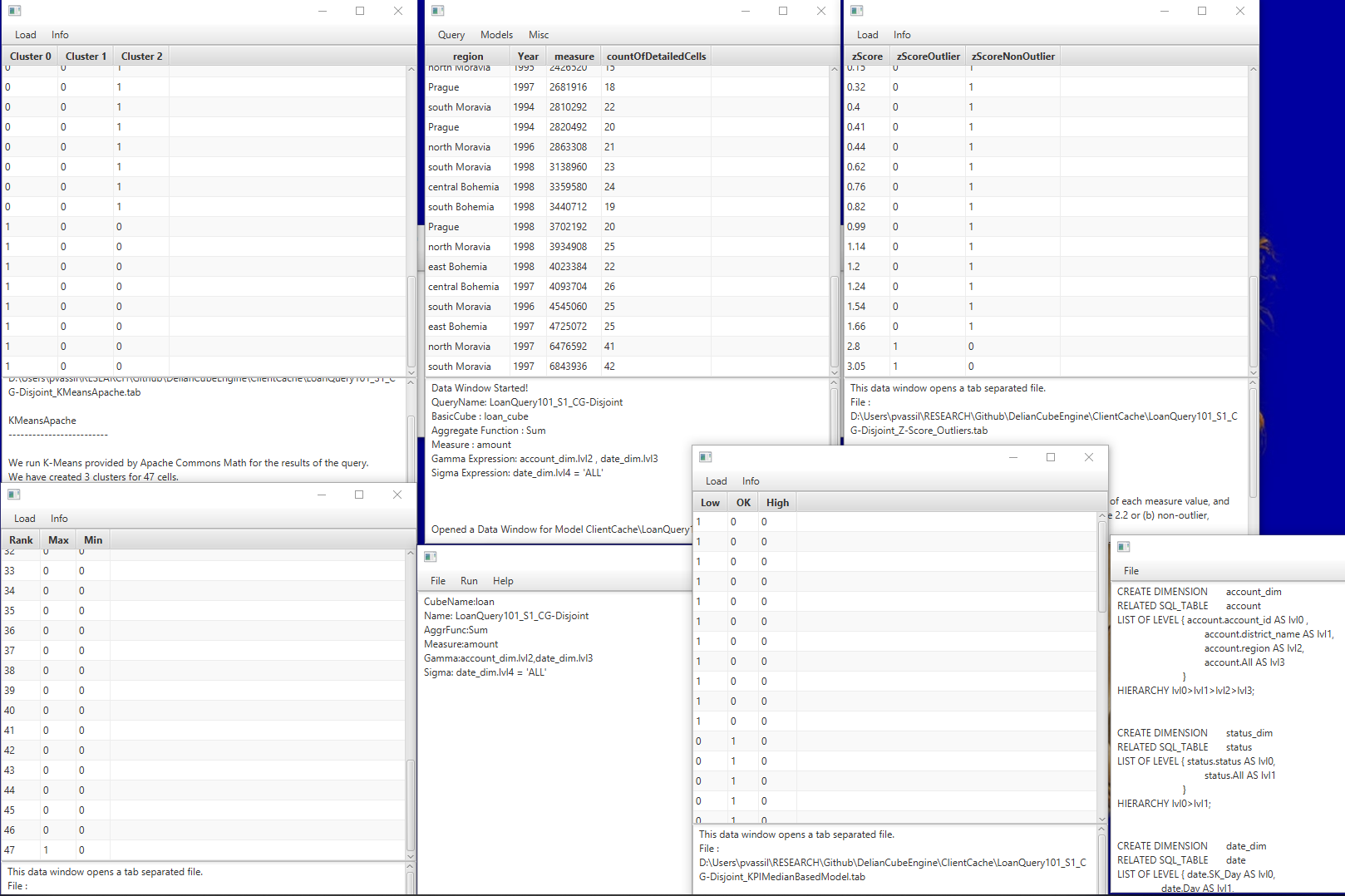
Figure 3: Delian Cube Engine: A dimension and cube description (bottom right), a cube query and its result (bottom and top middle, respectively) and a set of models and their model components as bitmaps.

Our Delian Cube Engine operates on top of a relational DBMS to support query answering and allows the registration of dimension hierarchies and cubes, in order to facilitate the answering of aggregate queries along the lines prescribed in the respective definition, involving selections on the levels, aggregations (and, internally, implicit joins of the fact to the dimension tables, in order to correctly construct the respective relational query). Practically, the user needs to map the tables of an underlying star schema to the respective dimension and cube structures. Once the cube dataset is registered and mapped to its underlying relational database, the system is ready to be queried. The user deals with cube queries, instead of using SQL, in a simple cube query language. The queries are passed from the front-end to the back-end of the engine for processing via an RMI connection. There, the following steps take place: (a) there is a model selection phase, where model extraction algorithms are selected to be applied on the results of the cube query, (b) there is a translation of the cube query into the respective SQL query that will actually be executed over the underlying database, (c) the resulting recordset is again translated back to cells and a cube is produced as an answer, (d) the selected model extraction algorithms are applied to the result of the query, (e) all the resulting cells, cubes, models, and model components are packaged and transferred back to the front-end for presentation (Fig. 3).

To assess the practicality of the method we have worked with a cubified version of the PKDD99 schema. The setup of both the client and the server parts, as well as the execution of all experiments, have been performed on a rudimentary laptop with an Intel i5-7200U CPU at 2.5GHz, 8GB install RAM, and a 512GB disk. We have worked with the original PKDD99 data set on bank loans, which is of small size, and artificially generated larger versions of it at 1M and 10M rows. The data set has a cube on loans; the amount loaned is the measure and the dimensions are accounts (generalized to geographical regions, with 3 levels), date, and status of the loan (practically single level). We execute a session that (1) starts by querying the entire cube, (2) focuses on the loan contracts that are running without problems, (3 and 4) compares drilled-down variants in terms of geography and date, and, finally, (5) re-focuses on a particular region where all contracts are queried. The execution of the queries is accompanied with the generation and execution of models: ranking, outlier detection, K-Means and KPI assessment.

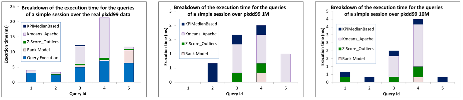
Figure 4: Breakdown of query and model execution time for the same query session, over different sizes for the same schema. All times are with hot cache.

The querying time scales linearly with the cube size, and we depict them only in the first of the sub-Figures of Fig. 4 to avoid visually suppressing the key message of the experiments which is found in the model generation and execution: in all cases, the model generation requires simply a few milliseconds (and frequently, fractions of them)! This is expected, as the models operate on the query result and not on the underlying cube. Thus, the psychological limit of 500 msec for producing an answer is not affected at all by the application of our models, in our experiment. We recognize that the visualizations employed are naïve, and thus fail to plug-in any time costs due to the visualization part —however, we consider this to be a matter of an open, wide field of research for the future.

6 Related work

6.1 Coupling data and models

The idea of coupling data and analytical models is not completely new. Already in the mid-90’s, inductive databases were proposed to couple data with patterns, i.e., generalizations extracted from the data. In this framework knowledge discovery is modelled as an interactive process in which users can query data as well as patterns using an ad hoc query language [33].

More specifically, in [16], among the research challenges in BI the authors emphasized the need to achieve a unified view of data and models that describe data, so that this two components can be used and queried together. The intuition proposed to move from data to models and vice-versa is that of folding data into models and unfolding models into data. Our approach goes exactly in this direction, being folding/unfolding achieved through the definition of components.

Some degree of data-to-model unification is actually achieved in MauveDB [34], which provides language constructs for declaratively specifying model-based views of data based on a variety of commonly used statistical models, meant as simplified descriptions of the underlying data. Though the authors recognize that the view definition has to be model-specific, they suggest to rely on the common aspects of different models to decrease the variation in the view-definition statements. They also indicate as the most promising approach to query processing over model-based views that of materializing an intermediate model-specific representation of the view. While their work is mostly focused on maintaining model-based views and transparently querying them in a SQL-like fashion, ours introduces intentional operators as a querying abstraction and uses highlights to emphasize relevant findings.

Most recently, the Northstar system has been proposed as a support to interactive data science [35]. Importantly, among the key requirements for interactive data science, the author mentions that of enabling users to seamlessly switch between data exploration and model building. To this end he developed the Alpine Meadow optimizer, which features a declarative language for machine learning tasks and a real-time strategy for hyper-parameter tuning.

6.2 Exploratory querying and data exploration

Interactive Database Exploration (IDE) is the process of exploring a database by means of a sequence of queries aiming at answering an often imprecise user information need. Typically, an exploration includes several queries where the result of each query triggers the formulation of the next one. Many approaches have recently been developed to support IDE, as illustrated by a recent survey of the topic [21]. In their survey, Idreos et al. adopt a top-down viewpoint and classify the existing approaches in three main categories: user interaction, middleware and database layer. Techniques range from visual optimization (like query result reduction [36]), automatic exploration (like query recommendation [27]), assisted query formulation (like data space segmentation [37]), data prefetching (like result diversification [38]) and query approximation [39].

One of the conclusion of this survey is that declarative “exploration” languages are still to be invented. We believe that the present work is a first step towards such a language.

OLAP exploration of data warehouses is a particular use case of database exploration that enables to work with simplifying assumptions, precisely, the multidimensional star schema or the regularities of multidimensional queries. Many approaches have been specifically developed to support OLAP exploration, as illustrated by the next subsection.

6.3 OLAP models and operators

The research on traditional models for OLAP and its operators (roll-up, drill-down, slice, drill-across) practically concluded around the turn of the millennium. We refer the interested reader to an excellent survey [2].

Apart from the traditional operators, related research has explored the possibility of providing operators with more knowledge extraction results. In an emblematic paper in the area, Sarawagi introduces the DIFF operator in [3], which returns a set of tuples that most successfully describe the difference of values between two cells of a cube that are given as input. The same author in [4] describes a method that profiles the exploration of a user and uses the Maximum Entropy principle to recommend which unvisited parts of the cube can be the most surprising in a subsequent query. In [5], Sathe and Sarawagi introduce the operator RELAX which verifies whether a pattern observed at a certain level of detail is also present at a coarser level of detail, too.

The Cinecubes method, introduced in [40] and [9] is aimed to provide automated reporting as a result to an original OLAP query. The proposed method enriches an original OLAP query with auxilliary queries to aid (a) the comparison and assessment of the result of the query to similar data and (b) the explanation of the result with values at the most detailed level. So, the result of the Cinecubes system can coarsely be grouped as the result of two operators: the first operator computes queries for values similar to ones defining the selection filters of the original query and the second one by drilling down into the dimensions of the result, one dimension at a time. The Cinecubes method also comes with the features of (a) (simple) highlight extraction, (b) packaging the result as a story, presented as a Powerpoint story, with text commenting on the highlights, audio produced automatically from the text and visualization of the query results in slides. We refer the interested reader to [9] which also includes the discussion of data narration and visualization, that is not covered here.

The Shrink operator [22, 23] goes in the direction of approximate query answering, whose main goal is to increase query efficiency by returning a reduced result while minimizing the approximation introduced. In particular, Shrink aims at balancing data precision with data size in cube visualization via pivot tables. To this end it takes as input a cube and compresses it to a given target size; this is done by fusing cube slices into a single representative slice, in such a way that the information loss is minimal. Other approaches to approximate query answering for OLAP are presented in [41, 42, 43].

Finally, in [10] the OLAP paradigm is reused to explore prediction cubes besides traditional data cubes. In a prediction cube, each cell summarizes a predictive model trained on the data corresponding to that cell. Specifically, each cell can measure either the accuracy of the model, or the similarity between two models, or the model predictiveness based on a test-set. This approach empowers decision making by supporting users in searching for interesting subsets of data in the light of a prediction model; however, differently from our approach, it does not identify highlights nor it provides a goal-oriented query language.

6.4 Query Recommendations

Query recommendation refers to the situation where (a) a user submits a query to the system and (b) the system follows up with suggesting subsequent queries to aid the user’s exploration. The suggestion can be based on the user’s profile, history of queries, history of other users’ queries, or other information. Query recommendation has recently attracted many attentions for Interactive Database Exploration [44, 27, 32] and particularly in the case of OLAP exploration of data cubes [45, 46, 47, 30, 31, 48, 49], including approaches applied to spatial OLAP [50, 51]. See [44, 52, 31, 53] for a broader discussion.

As it is the case for general purpose recommender systems, query recommendation methods can be classified into content-based approaches, collaborative approaches, or combination thereof. Content-based approaches compute suggestions based on the data seen by the user and and unseen data. For instance, Cariou et al., in [28] describe a method that mines the most interesting dimension for a user to explore, based on his history. As already mentioned, a similar problem has been addressed in [4]. Jerbi et al. [45] propose an approach where recommendations are computed based on the navigation context and preferences stated in the user profile. Collaborative approaches take advantage of the wisdom-of-the-crowd effect. The authors of [47, 31] use the query log of previous users to find similar queries which can give information to user who may not know it is available. Drushku et al. [49] use the query log of previous users to detect user intents and recommend queries that fit the user’s current intents.

As explained in Section 4, our suggest intention encapsulates these recommendation strategies in their variety.

6.5 Intensional querying

Non-conventional query answering includes a variety of answering mechanisms and happens when either the user has no clear formulation of his needs (e.g., he does not know what he really wants) or has a good understanding of his needs but is flexible enough to accept an alternate, approximate or intensional answer. Among several kind of non-conventional answers, we distinguish intensional query answering as the more relevant to our work. According to [54], an intensional query answer complements the extensional one by including either a concise description of the answer or some useful facts about it.

Intensional query answering relies generally on knowledge like integrity constraints, inference rules (in knowledge-based systems), ontology (and more frequently a taxonomy), and user’s preferences to either provide more insight about the extensional answer or give an approximate answer.

Intensional query answering has been applied in many area of computer science (e.g., object-oriented databases [55], deductive database [56], and question answering systems [57, 58]) but, to the best of our knowledge, the only work related to the OLAP area is [59], that proposes a framework for computing an intensional answer to an OLAP query by leveraging the previous queries in the current session. The idea is to use an intensional answer to concisely characterize the cube regions whose data do not change along the sequence, coupled with an extensional answer to describe in detail only the cube regions whose data significantly differ from the expectation.

6.6 Interestingness

As explained in Section 3, our approach for highlight selection based on a significance score is inspired by the framework for subjective interestingness in exploratory data mining proposed by De Bie [19]. The framework is based on the idea that the goal of the explorative pattern mining is to pick patterns that will result in the best updates of the user’s belief state, while presenting a minimal strain on the user’s resources. In this sense, an interestingness measure (IM) is subjective in that it depends on the belief of the explorer. A general definition for this IM is a real-valued function of a background distribution (that represents the belief) and a pattern (the artifact to be presented to the explorer). The belief is the probability P$(\omega)$ of the event $x\in\omega$, i.e., the degree of belief the user attaches to a pattern (characterized by $\omega$) being present in the data $x$. In other words, if this probability is small, then the pattern is subjectively surprising for the explorer. The data mining process consists of extracting patterns and presenting first those that are subjectively surprising, and then refining the belief. Our principle of highlight selection is inspired by this framework, in the sense that the highlights to be selected maximize the surprise caused by confronting a significance score computed for the initial cube (that can be thought of as the user belief) with the significance score computed for the target cube to select a model component (that can be thought of as the pattern to be presented).

6.7 Principles behind the foundation of our operators

The foundations of what are the basic operators that users perform during OLAP and data exploration have been a really difficult problem in our search. The related literature that we could find does not particularly help towards this direction.

We start by observing that our approach goes in the direction of reducing the number of interactions a user needs to achieve her analysis goals. Specifically, with reference to the Observation-Orientation-Decision-Action loop applied to BI [60], intentional analytics empowers both the observation phase (look at the data with an expectation of what it should be) and the orientation phase (we look at the data in different ways depending on what it shows).

Interestingly, intent-driven query formulation in the OLAP context has been investigated to some extent in [61], which proposes meta-morphing as a way to have incomplete user queries completed by the system based on the previous interactions of that user. This approach is different from ours mainly in two ways: (i) an intention for us is not an incomplete query but a high-level analytical goal, and (ii) query answers for us encompass both data and models.

In [62] the authors perform a semi-structured interview with 25 analysts to understand what data analysis and visualization entails as a process. The authors come up with 5 high-level tasks: discovery, wrangling, profiling, modeling and reporting of information. Expectedly (at least for the educated data warehouse experts) discovery and wrangling of data are the most tedious of the tasks. However, when it comes to the environment of OLAP, which is performed over simply-but-neatly organized cubes, these two tasks, along with profiling (i.e., data quality assurance) have already been completed, either by the organization ETL workflow, or by a do-it-yourself data wrangling. The rest of the high-level tasks are too few and too high for our purpose here.

In a similar vein, in [63], the authors propose a taxonomy of user tasks in exploratory data analysis that include (1) discovery (hypothesis formulation and determination of the data source that can answer it) , (2) data acquisition (and preparation), (3) exploration of the data, (4) modeling, via the construction of a model that explains the data, and, (5) communication of the results to other people via reports and presentations. The discussed taxonomy is very close to the one presented in [62] , but similarly suffers from the high-level of abstraction for the exploration part. Having said that, we also say that we are very close to the fundamental principle of working with data that this paper outlines: once the data are ready, users explore to find out what the status is and to understand the data, and construct models that explain the phenomena – what we add is more detail on the exploration and, notably, automation of the process.

Another path that we followed was to search for foundations for on-line search in the web, which is a similar area. In [64] the authors conduct a user study of 72 participants engaged in 426 user tasks and deduce it is worthwhile to deduce the intentions that drive the users to perform their searches. We quote from the abstract of the paper: ”The implication of this research is that rather than solely addressing a searcher’s expressed information need, searching systems can also address the underlying learning need of the user.” After a detailed survey of the literature on learning styles, the authors suggest that the best candidate to serve as the foundation of the learning tasks of users is the cognitive learning framework that was proposed by Anderson and Krathwohl as a refinement to Bloom’s taxonomy.

It is worthwhile to discuss Bloom’s taxonomy and Anderson and Krathwohl’s refinement to it [65], [66]. The framework tries to categorize the different domains of human learning (mainly with a view to children education), and includes the following main cognitive tasks: (a) remembering, (b) understanding (by extracting meaning out of messages or activities), (c) applying the material learned via a procedure, (d) analyzing by understanding how the different parts of artifacts or concepts relate to each other, (e) evaluating based on criteria and standards, (f) creating of new artifacts by composing individual pieces into a coherent or functional assembly. Our framework, tries to automate the remembering and application, but at the same time retains the understanding (via the description of the status in different ways and levels of abstraction), the analysis (via the explanations provided) and the evaluation parts. We cover the creation part at the future work section.

6.8 Relationship to our previous work

A first version of this paper appears in [18]. The largest part of [18] is included in Section 1.2. The rest of the contents of the paper are completely novel. The initial set of intentional operators of [18] has been abstracted further in this paper and replaced by the operators of Section 4. The parts on the model’s definition and the interestingness evaluation are not covered in [18].

7 Conclusions and paths for future research

This paper is a vision paper describing, in broad terms, a potential future for OLAP, to strengthen its place as the corner stone of BI. We are convinced that, after 50 years of query answering, it is now time to replace it with effortless, automatic insight gaining from the user. Instead of making the end user dig into sets of records, we can increase productivity and the understanding of the essence of the data by using two pillars, one devoted to querying (i.e., what an OLAP query is), and another devoted to answering (i.e., what the answer to an OLAP query is). Specifically, firstly, we want to allow the user to focus on high-level goals of information acquisition, rather than details of what data to bring in, and secondly, to automatically suggest focus-points in the answers that will move the user effort from manual ”jewel mining” to addressing the insights gained.

Beyond the proposed new viewpoint to OLAP, our call to arms to the research community involves several open roads for research.

New intentional operators. In this paper we have proposed a set of fundamental operators for the OLAP tools of the close future. New operators, esp., as combinations of old ones can also be devised. We would assume as a pre-requisite for each such operator to come with a graceful linkage to the overall model proposed here (in an attempt to be able to gracefully plug it in the respective BI tools under a uniform setting).

Alternatives for full automation. Much like in traditional query processing, the intentional operators can come with alternative execution algorithms for the data collection and the model construction, in order to facilitate the optimization of the task. The optimization can be thought, not only in terms of performance, but also in terms of information content delivered. Of course, the fine tuning of any algorithms concerning their parameter fixing is also important.

Optimization concerns. In practice, intentional operators can be envisioned as sequences of different logical OLAP and ML operators. Besides, the cube resulting from each logical operator can be enhanced with highlights obtained by applying different algorithms (e.g., clustering or classification). Thus, much like for the selection of an execution plan for a SQL query, executing an intentional operator requires an optimization phase to decide which logical operators and model mining algorithms to execute. How exactly this optimizer will be structured internally, and what optimization algorithms and tunings will be employed is clearly a topic of future research.

Packaging into data stories. In this paper we have focused on the deeper layers of query answering, which involves data acquisition and mining. The visual representation of all these results, the automatic choice of graphical representation, the automatic generation of data stories and the overall packaging to the user are topics that, despite their importance, have traditionally been outside the walls of the database community, mainly due to the difficulty of experimentally verifying the effectiveness of any proposed method. Still, answers to the automation of the aforementioned tasks are highly valuable and pose open research topics.

Benchmarking and tools. A free, open-source (FOSS) tool and a reference benchmark for the future BI (involving data, model, and highlight extraction requests and sessions) can be a really handy tool for the research community (otherwise, each new paper will need to improvise on its experimental assessment). A tool will also trigger other research directions like, e.g., the incorporation of research results on natural language processing to accept the user requests, new visualizations to show models and highlights, etc.

Acknowledgments. We are particularly thankful to the reviewers of both this paper and its preliminary version in DOLAP 2018 for their comments that helped us enrich the breadth of the related work, and the clarity of concepts and terminology.

APPENDIX

8 Formalizing data, dimension hierarchies cubes and cube queries

An OLAP session is a sequence of dashboards that the analyst sees, each with its own information, including data, charts and informative summaries of KPI performance. The sequence is produced by the actions of the analyst that changes the contents of the dashboard by requesting more information on the basis of a set of operations made available to him by the tool.

8.1 Preliminaries on multidimensional modeling

In this Section, we give the formal background of our modeling concerning multidimensional databases, hierarchies and queries. We closely follow the model of [9] and slightly extend it. As typically happens with multidimensional models, we assume that dimensions provide a context for facts [8]. This is especially important considering that dimension values come in hierarchies; every single fact can be simultaneously placed in multiple hierarchically-structured contexts, thus giving users the possibility of analyzing sets of facts from different perspectives. The underlying data sets include measures that are characterized with respect to these dimensions. Cube queries involve measure aggregations at specific levels of granularity per dimension, along with filtering of data for specific values of interest.

8.2 Domains, dimensions and underlying data

Domains. We assume the following infinitely countable and pairwise disjoint sets: a set of level names (or simply levels) $\mathcal{U_{L}}$, a set of measure names (or simply measures) $\mathcal{U_{M}}$, a set of regular data columns $\mathcal{U_{A}}$, a set of dimension names (or simply dimensions) $\mathcal{U_{D}}$ and a set of cube names (or simply cubes) $\mathcal{U_{C}}$. The set of data columns $\mathcal{U}$ is defined as $\mathcal{U}$ = $\mathcal{U_{L}}$ $\cup$ $\mathcal{U_{M}}$ $\cup$ $\mathcal{U_{A}}$. For each $L$ $\in$ $\mathcal{U_{L}}$, we define a countable totally ordered set $dom(L)$, the domain of $L$, which is isomorphic to the integers. Similarly, for each $M$ $\in$ $\mathcal{U_{M}}$, we define an infinite set $dom(M)$, the domain of $M$, which is isomorphic either to the real numbers or to the integers. The domain for the regular data columns of $\mathcal{U_{A}}$ is defined in a similar fashion to the one of measures. We can impose the usual comparison operators to all the values participating to totally ordered domains ${\{}<,>,\leq,\geq{\}}$.

Dimensions and levels.A dimension $D$ is a lattice ($\mathbf{L}$,$\prec$) such that:

• $\mathbf{L}$ = $\{$$L_{1}$,$\ldots$ ,$L_{n}$$\}$, is a finite subset of $\mathcal{U_{L}}$.

• $dom(L_{i})$ $\cap$ $dom(L_{j})$= $\emptyset$ for every $i$ $\neq$ $j$.

• $\prec$ is a partial order defined among the levels of $\mathbf{L}$.

• With $D$ being a lattice, it follows that there is a highest and a lowest level in the hierarchy. The highest level of the hierarchy is the level $D$.$ALL$ with a domain of a single value, namely ’$D$.$all$’. Moreover, there is also the lowest level in the dimension, $D.L_{\perp}$, for which there does not exist any other level $L$’ in $\mathbf{L}$, such that $L$’ $\prec$ $L_{\perp}$.

Each path in the dimension lattice, beginning from its upper bound and ending in its lower bound is called a dimension path. The values that belong to the domains of the levels are called dimension members, or simply members (e.g., the values $Paris$, $Rome$, $Athens$ are members of the domain of level $City$, and, subsequently, of dimension $Geography$).

To ensure the consistency of the hierarchies, a family of functions $anc_{L_{1}}^{L_{2}}$ is defined, satisfying the following conditions:

1. For each pair of levels $L_{1}$ and $L_{2}$ such that $L_{1}$ $\prec$ $L_{2}$, the function $anc_{L_{1}}^{L_{2}}$ maps each element of $dom(L_{1})$ to an element of $dom(L_{2})$.

2. Given levels $L_{1}$, $L_{2}$ and $L_{3}$ such that $L_{1}$ $\prec$ $L_{2}$ $\prec$ $L_{3}$, the function $anc_{L_{1}}^{L_{3}}$ equals to the composition $anc_{L_{1}}^{L_{2}}$ $\circ$ $anc_{L_{2}}^{L_{3}}$. This implies that:

   • $anc_{L_{1}}^{L_{1}}(x)$ = $x$.

   • if $y$ = $anc_{L_{1}}^{L_{2}}(x)$ and $z$ = $anc_{L_{2}}^{L_{3}}(y)$, then $z$ = $anc_{L_{1}}^{L_{3}}(x)$.

   • for each pair of levels $L_{1}$ and $L_{2}$ such that $L_{1}$ $\prec$ $L_{2}$, the function $anc_{L_{1}}^{L_{2}}$ is monotone (preserves the ordering of values). In other words:

     $\forall$ $x$,$y$ $\in$ $dom(L_{1})$: $x$ $<$ $y$ $\Rightarrow$ $anc_{L_{1}}^{L_{2}}(x)$ $\leq$ $anc_{L_{1}}^{L_{2}}(y)$, $L_{1}$ $\prec$ $L_{2}$

3. For each pair of levels $L_{1}$ and $L_{2}$ such that $L_{1}\prec L_{2}$ the $anc_{L_{1}}^{L_{2}}$ function determines a set of finite equivalence classes $X_{i}$ such that:

   $$(\forall x,y\in dom(L_{1}))\ (anc_{L_{1}}^{L_{2}}(x)=anc_{L_{1}}^{L_{2}}(y)\Rightarrow x~{}and~{}y\mbox{ belong to the same }X_{i}).$$

4. The relationship $desc^{L_{2}}_{L_{1}}$ is the inverse of the $anc_{L_{1}}^{L_{2}}$ function, i.e.,

   $$desc^{L_{2}}_{L_{1}}(l)=\{x\in dom(L_{1}):anc_{L_{1}}^{L_{2}}(x)=l\}.$$

Level properties. Levels are also annotated with properties. For each level $L$, we define a finite set of functions, which we call properties, that annotate the members of the level. So, for each level $L$, we define a finite set of functions $\mathcal{F}^{L}$ = $\{F^{L}_{1},~{}\ldots,~{}F^{L}_{k}\}$, with each such function $F^{L}_{i}$ mapping the domain of $L$ to a regular data column $A_{i}$, s.t., $A_{i}$ $\in$ $\mathcal{U_{A}}$, i.e., $F^{L}_{i}$: $dom(L)$ $\rightarrow$ $dom(A_{i})$. So, for example, for the level $City$, we can define the functions $population()$ and $area()$. Then, for the value $Paris$ of the the level $City$, one can obtain the value $2M$ for $population(Paris)$ and $100Km^{2}$ for $area(Paris)$.

Schemata. First, we define what a schema is in a multidimensional space.

A schema $\mathbf{S}$ is a finite subset of $\mathcal{U}$.

A multidimensional schema is divided in two parts: $\mathbf{S}$ = [$D_{1}$.$L_{1}$, $\ldots$, $D_{n}$.$L_{n}$, $M_{1}$, $\ldots$, $M_{m}$], where:

• $\{$$L_{1}$,$\ldots$ ,$L_{n}$$\}$ are levels from a dimension set $\mathbf{D}$ = $\{$$D_{1}$,$\ldots$, $D_{n}$$\}$ and level $L_{i}$ comes from dimension $D_{i}$, for 1 $\leq$ $i$ $\leq$ $n$.

• $\{$$M_{1}$,$\ldots$, $M_{m}$$\}$ are measures.

A detailed multidimensional schema $\mathbf{S}^{0}$ is a schema whose levels are the lowest in the respective dimensions.

Facts and cubes. Now we are ready to define what a fact is, expressed as a cell, or multidimensional tuple in the multidimensional space.

A tuple under a schema $\mathbf{S}$ = [$A_{1}$, $\ldots$, $A_{n}$] is a point in the space formed by the Cartesian Product of the domains of the attributes $A_{i}$, $dom(A_{1})$ $\times$ $\ldots$ $\times$ $dom(A_{n})$, such that $t[A]$ $\in$ $dom(A)$ for each $A$ $\in$ $\mathbf{S}$.

A multidimensional tuple, or equivalently, a cell or a fact, $t$ is a tuple under a multidimensional schema $\mathbf{S}$ = [$D_{1}$.$L_{1}$, $\ldots$, $D_{n}$.$L_{n}$, $M_{1}$, $\ldots$, $M_{m}$].

Having expressed what individual pieces of data, or facts, are, we are now ready to define data sets and cubes .

A data set $\mathbf{DS}$ under a schema $\mathbf{S}$ = [$A_{1}$, $\ldots$, $A_{n}$] is a finite set of tuples under $\mathbf{S}$.

A multidimensional data set $\mathbf{DS}$, also referred to as a cube, under a schema $\mathbf{S}$ = [$D_{1}$.$L_{1}$, $\ldots$, $D_{n}$.$L_{n}$, $M_{1}$, $\ldots$, $M_{m}$] is a finite set of cells under $\mathbf{S}$ such that:

• $\forall$ $t_{1}$, $t_{2}$ $\in$ $\mathbf{DS}$, $t_{1}$[$L_{1}$,$\ldots$, $L_{n}$] = $t_{2}$[$L_{1}$, $\ldots$, $L_{n}$] $\Rightarrow$ $t_{1}$ = $t_{2}$.

• for no strict subset $X$ $\subset$ ${\{}L_{1},\ldots,L_{n}{\}}$, the previous also holds.

In other words, $M_{1}$, $\ldots$, $M_{m}$ are functionally dependent (in the relational sense) on levels $\{$$L_{1}$,$\ldots$ ,$L_{n}$$\}$ of schema $\mathbf{S}$.

A detailed multidimensional data set $\mathbf{DS}^{0}$ is a data set under a detailed schema $\mathbf{S}^{0}$.

A star schema ($\mathbf{D}$,$\mathbf{S}^{0})$ is a couple comprising a finite set of dimensions $\mathbf{D}$ and a detailed multidimensional schema $\mathbf{S}^{0}$ defined over (a subset of) these dimensions.

Example 13

Consider the detailed data set $DS$ displayed in Figure 5, coming from the well known Adult (a.k.a census income) dataset referring to data from 1994 USA census. There are 8 dimensions (Age, Native Country, Education, Occupation, Marital status, Work class, Race and Gender) in the data set and a single measure, Hours per Week. Each dimension comes with a lowest possible level, which we denote as $L_{0}$. Being a multidimensional data set, immediately makes $DS$ a detailed cube, so in the subsequent discussions, $DS$ will also be referred to as $C^{0}$. This detailed data set will be the basis of our running example.

Figure 5: A subset of the detailed data set $DS$ (equiv., $C^{0}$), with its 8 dimensions at the lowest possible level of detail and its single measure (depicted in the last column).

8.3 Selections

Selection filters. An atom is $true$, $false$, (with obvious semantics) or an expression of the form $anc_{L_{0}}^{L_{1}}(L_{1})$ $\theta$ $v$, or in shorthand, $L_{1}$ $\theta$ $v$, with $v$ $\in$ $dom(L_{1})$. $\theta$ is an operator from the set $\{>,<,=,\geq,\leq,\neq\}$.

A selection condition $\phi$ is a formula involving atoms and the logical connectives $\wedge$, $\vee$ and $\neg$. A well-formed selection condition is defined as a selection condition that is applied to a data set with all the level names that occur in it belonging to the schema of the data set. In the rest of our deliberations, we assume that all the selection conditions are well-formed, unless specifically mentioned otherwise. The expression $\phi(\mathbf{DS})$ is a set of tuples $\mathbf{X}$ belonging to $\mathbf{DS}$ such that when, for all the occurrences of level names in $\phi$, we substitute the respective level values of every $x$ $\in$ $\mathbf{X}$, the formula $\phi$ becomes true.

A detailed selection condition $\phi^{0}$ is a selection condition where all participating levels are the detailed levels of their dimensions.

8.4 Cube queries

Cube queries. The user can submit cube queries to the system. A cube query specifies (a) the detailed data set over which it is imposed, (b) the selection condition that isolates the records that qualify for further processing, (c) the aggregator levels, that determine the level of coarseness for the result, and (d) an aggregation over the measures of the underlying cube that accompanies the aggregator levels in the final result. More formally, a cube query, is an expression of the form:

$$c=\langle\ \mathbf{DS}^{0},\ \phi^{0},\ [L_{1},\ldots,L_{n},M_{1},\ldots,M_{m}],\ [agg_{1}(M^{0}_{1}),\ldots,agg_{m}(M^{0}_{m})]\ \rangle$$

where

1. $\mathbf{DS}^{0}$ is a detailed data set over the schema $\mathbf{S}$ =[$L_{1}^{0}$, $\ldots$, $L_{n}^{0}$, $M_{1}^{0}$, $\ldots$ ,$M_{k}^{0}$], $m$ $\leq$ $k$.

2. $\phi^{0}$ is a detailed selection condition,

3. $L_{1},\ldots,L_{n}$ are levels such that $L^{0}_{i}\prec L_{i}$, $1\leq i\leq n$,

4. $M_{1},\ldots,M_{m}$, $m\leq k$, are aggregated measures (without loss of generality we assume that aggregation takes place over the first $m$ measures – easily achievable by rearranging the order of the measures in the schema),

5. $agg_{1},\ldots,agg_{m}$ are aggregate functions from the set $\{sum,$ $min,max,count\}$.

The semantics of a cube query in terms of SQL over a star schema are:

SELECT $L_{1}$,…,$L_{n}$, $agg_{1}(M_{1}^{0})$ AS $M_{1}$,…,$agg_{1}(M_{m}^{0})$ AS $M_{m}$

FROM DS0 NATURAL JOIN D1 … NATURAL JOIN Dn

WHERE $\phi^{0}$

GROUP BY $L_{1}$,…,$L_{n}$

where $D_{1}$, $\ldots$, $D_{n}$ are the dimension tables of the underlying star schema and the natural joins are performed on the respective surrogate keys

A cube query specifies (a) the cube over which it is imposed, (b) a selection condition that isolates the facts that qualify for further processing, (c) the grouping levels, which determine the coarseness of the result, and (d) an aggregation over some or all measures of the cube that accompanies the grouping levels in the final result.

Interestingly, a cube query carries the typical duality of views: it is, at the same time, both a query, as it involves a query expression imposed over the underlying data, but, also a cube, as it computes a set of cells as a result that obey the constraints we have imposed for cubes.

Example 14

The following cube query produces the cube of Table 16: $C^{N}=\langle DS,$

education.L3=’Post-secondary’ and work_class.L2=’With-Pay’,

$\langle$ALL,ALL,L2,ALL,L0,ALL,ALL$\rangle,$

$Avg(Hours~{}per~{}Week)\rangle$

where $DS$ is the detailed data set, the selection condition fixes Education to ’Post-Secondary’ (at level L3), and Work to ’With-Pay’ (at level L2), data is grouped by Education at level 2, and Work at level 1, and the Avg of Hours per Week is requested.

Hrs per Week	Assoc	Post-grad	Some-college	University
Federal-gov	41.15	43.86	40.31	43.38
Local-gov	41.33	43.96	40.14	42.34
State-gov	39.09	42.96	34.73	40.82
Private	41.06	45.19	38.73	43.06
Self-emp-inc	48.68	53.05	49.31	49.91
Self-emp-not-inc	45.88	43.39	44.03	44.44

Table 16: A new cube $C^{N}$ as the output of the cube query of Example 14

For the reader familiar with OLAP terminology, the new cube $C^{N}$ resulting from the query, is practically the result of a Drill-Down operation over the old cube $C^{O}$ of Example 1.

The expression characterizing a cube has the following formal semantics:

$$\begin{array}[]{l}c=\mbox{\{}\ x\ |\mbox{(}\exists y\in\phi^{0}(DS^{0}))\ (x=(anc^{L_{1}}_{L^{0}_{1}}(y[L^{0}_{1}]),\ldots,anc^{L_{n}}_{L^{0}_{n}}(y[L^{0}_{n}]),\ agg_{1}\{G_{1}\},\ldots,agg_{m}\{G_{m}\})\mbox{)}\mbox{\ }\}\end{array}$$

where for every $i$ ($1$ $\leq$ $i$ $\leq$ $m$) the set $G_{i}$ is defined as follows:

$$\begin{array}[]{l}G_{i}=\mbox{\{}\ q\ |\mbox{(}\exists z\in\phi^{0}(DS^{0}))\ (x[L_{1}]=anc^{L_{1}}_{L^{0}_{1}}(z[L^{0}_{1}]),\ldots,x[L_{n}]=anc^{L_{n}}_{L^{0}_{n}}(z[L^{0}_{n}]),q=z[M^{0}_{i}]\mbox{)}\ \mbox{\}}\end{array}$$

9 Formalizing Algorithms

To be able to compute the results of model and highlight extraction algorithms, we resort to the modeling of algorithms as functions. We will present a simple taxonomy of algorithms in the context of our cube model and then, we will proceed to define the formalization of algorithms as black-box functions. In our subsequent deliberations, we will discuss how algorithms facilitate the extension of database-generated query results with (a) simple computations over the query results, (b) model extraction data mining algorithms, and (c) highlight extraction algorithms isolating the important results of the previous computations for the dashboard state.

9.1 Algorithms as functions and a taxonomy of functions

Taxonomy. Specifically, we classify algorithms (remember: practically, functions) in three classes:

• Cell-based algorithms. These algorithms operate locally on a cell, independently of the rest of the contents of the input cube. Simple arithmetic computations belong to this category (e.g., $profit$ = $price$ - $cost$).

• Subcube-based algorithms. These algorithms can operate by splitting the input cube to equivalence classes, which we call subcubes, according to some criterion. Then, the computation of the new attributes for the cells of the subcube, require the entire sub-cube to be fed to the algorithm as input. Take for example, (a) a time series decomposition algorithm producing three new attributes for each input cell (specifically, $trend$, $seasonality$ and $noise$), and, (b) a cube of $Sales$ that is grouped per $Product$ and $Month$. Each product, then, defines a time series. Thus, the algorithm can split the input to a set of subcubes, one per product and perform time series decomposition for each of its cells. Again, notice that although, ultimately, each cell gets its own values: (a) we cannot compute the new cell values by looking at each cell in isolation, and on the other hand, (b) we do not need the entire cube to compute them, but only the set of values that pertain to the same time series.

• Cube-based algorithms. These algorithms require the entire cube to be present for the computation of a cell’s extra attribute. Examples of this kind of algorithms range from very simple algorithms, like determining the bottom 3 values of a cube to highly sophisticated algorithms like outlier detection or Fourier analysis.

Given a data set $D$, and a tuple $x$ belonging to $D$, an algorithm $f$, depending on its category, induces an equivalence class relation $eqClass_{f}(x)$ producing a set of tuples that include (a) only $x$ for a cell-based algorithm $f$, (b) all $D$ for a cube-based $f$, and (c) a subset of $D$, depending on the semantics of $f$, in the case of subcube-based $f$.

Algorithms as Functions. We adopt a traditional modeling of algorithms, which treats an algorithm, or equivalently, a function as a triplet involving the following signature :

• a algorithm name, say $f$

• a vector of input parameters, say $X$ = $\langle X_{1},\ldots,X_{I}\rangle$

• a vector of output parameters, say $Y$ = $\langle Y_{1},\ldots,Y_{O}\rangle$

To model algorithms and parameters, we assume a countable set of data computation function names $\mathcal{U_{F}}$ and a countable set of parameter names $\mathcal{U_{P}}$, which is a subset of the names appearing in $\mathcal{U_{A}}$. Each parameter $A$, input or output, is accompanied by a domain, $dom(A)$. We will refer to $X$ as the input schema of the algorithm and to $Y$ as the output schema of the algorithm. Then, the algorithm is a relation mapping $dom(X_{1})$ $\times$ $\ldots$ $\times$ $dom(X_{I})$ to $dom(Y_{1})$ $\times$ $\ldots$ $\times$ $dom(Y_{O})$.

The call of an algorithm requires fixing a data set over which the algorithm will be applied and the assignment of the input parameters of the algorithm to columns of the data set or constants. The latter is done by assigning to them (a) constant values (without loss of generality we assume constants belonging to $\mathbb{R}$), or, (b) data columns from a data set. Given an underlying data set, a valid parameter binding of an algorithm to the data set is a total mapping $B$: $X$ $\rightarrow$ $\mathcal{U}$ $\cup$ $\mathbb{R}$ that uses only constants and data columns of the data set, respecting also the compatibility of the domains between the algorithm signature and the members of the binding. Unless explicitly mentioned, all our parameter bindings of algorithms to cube queries are valid. We denote the binding $B$ of a algorithm $f$ to a data set $D$ and a valid binding of its input parameters $B(X)$ as $B(X|D)$.

Once such a binding has been done, the execution of a algorithm produces a set of tuples abiding by the output schema $Y$. To denote the execution of the algorithm we will use the notation $D^{+}$ = $f_{D}^{B(X)}$.

Assuming a data set $D$ under the schema $X$ and a algorithm $f$: $X$ $\rightarrow$ $Y$, the extended data set $D^{+}$ resulting from the execution of $f$ under a binding $B(X|D)$ is defined as follows:

• The schema of $D^{+}$ is $S$ = $X$ $\cup$ $Y$

• For each tuple $x$ $\in$ $X$, there is exactly one tuple $s$ in $D^{+}$, such that $s[X_{1},\ldots,X_{I}]$ = $x[X_{1},\ldots,X_{I}]$ and $s[Y_{1},\ldots,Y_{O}]$ = $f_{D}^{B(X)}$($eqClass_{f}(x))$

• No tuples other than the aforementioned belong to $D^{+}$

Observe, that we want to annotate each input tuple with a set of output values, independently of whether the algorithm is cell-based or not. In the case of cell-based algorithms, $f_{D}^{B(X)}(x)$ ignores the other tuples of $D$ and uses only $x$, whereas in the case of subcube-based algorithms it uses only the subcube of $x$. This also means that each time, a tuple $x$ gets the same result with its equivalence class.

Whenever the details of the binding are not important, we will use a shorthand notation $D^{+}$ = $f(D)$.

An extended cube query $c^{+}$ produced by the application of a algorithm $f$ to a cube query $c$ under the schema [$L_{1}$, $\ldots$, $L_{n}$, $M_{1}$, $\ldots$, $M_{m}$], i.e., $c^{+}$ = $f(c)$, comes with the same semantics as data sets.

9.2 The generating data of a dashboard

As we will demonstrate in the sequel, a dashboard includes a set of queries. We can exploit the raw generating data of the dashboard (i.e., the data that come from the underlying database via database queries), to produce derived values for each of the cells of a cube query, via the application of simple data computing functions. The produced cells are the generating data of the dashboard.

We employ the term cube query set, or for short, query set for a finite set of queries $C$ = ($c_{1}$, $\ldots$, $c_{k}$). Assuming a query set $C$ = ($c_{1}$, $\ldots$, $c_{k}$) for a dashboard $S$, the results of the queries of $C$ are the raw generating data of $S$. Similarly to query sets, an extended query set $C^{+}$ = ($c_{1}^{+}$, $\ldots$, $c_{k}^{+}$) is a finite set of extended queries, providing the generating data of $S$.

9.3 Algorithm and function composition

The composition $f\circ g$ of two algorithms $f$ and $g$ carries the same semantics and constraints as the composition of functions in mathematics. The composition of a list of algorithms $f_{1}$, $\ldots$, $f_{n}$ is a repetitive application of the composition operator (($\ldots$($f_{1}\circ f_{2}$) $\ldots$ $\circ$ $f_{n-1}$) $\circ$ $f_{n}$).

For the sake of generality, we can also compute the composition of individual data computing algorithms over simple cube queries. Assume a cube query $c$ under the schema [$L_{1}$, $\ldots$, $L_{n}$, $M_{1}$, $\ldots$, $M_{m}$]. Assume also the composition of a list of algorithms $\mathcal{F}$ = $f_{1}$, $\ldots$, $f_{n}$. We say that the composition of the algorithms’ list has a valid binding to the cube query $c$ when each algorithm $f_{i}$ has a valid binding to the result of the composition $f_{1}$ $\circ$ $f_{2}$ $\circ$ $\ldots$ $\circ$ $f_{i-1}$ applied over $c$. The schema and the contents of the extended cube query produced $c^{+}$ by the application of $f_{1}$ $\circ$ $f_{2}$ $\circ$ $\ldots$ $\circ$ $f_{n}$ to $c$ are produced as defined above.

10 Formalities for models

10.1 General Principles

Having defined data and algorithms, we ca now proceed to discuss the computation of statistical models from the data. We are going to treat model construction algorithms as ”black-box” functions without probing into their internals, and, most importantly, without assuming any specialized properties for their output. What does a model construction algorithm do? Basically, the algorithm receives as input (a) a set of input data, and, (b) a set of execution parameters that have to be fixed for the algorithm’s execution. Without loss of generality, we can assume that a subset of these parameters will be bound to string or numerical values and the rest will be mapped to attributes of the input data. The output of a model construction algorithm is a model of the input data. Depending on the algorithm, the result differs. For instance, a descriptive model built using unsupervised clustering is basically just a labeling of each cube’s cells, while a predictive one allows enriching the cube with predictions and comes with an accuracy score. In summary, the main properties of a model construction algorithm are outlined as follows:

1. Input: a set of input data, which is the result of an extended cube query set of the dashboard, along with a binding of the algorithm’s input parameters.

2. Output: a (possibly complex) result composed of (a) a model of the input data, and, (b) several characterizations of it (precision, strength, p-value, etc.).

Models are produced as instances of model types. A model is a concise representation of some knowledge about the data. This knowledge can be some relationship between data attributes, some property or characterization of subsets of data, or some computed value over the existing data. At the same time, despite its conciseness, typically a model also serves as an enrichment of the underlying data – in other words, conceptually, each record of the data can be extended, annotated, or, in any case, enriched with extra information by the model. We do this by organizing models as sets of model components, with each model component having exactly one value for each of the cells of the model’s generating data. This is what we refer to as data-to-model mappings.

10.2 Model Types

Every model construction algorithm has a result type: after the execution of the algorithm, its output, i.e., the resulting model of the input data is bound to this result type. To facilitate the management of models, we assume an infinitely countable domain of data type names $\mathcal{U_{T}}$, each member of which, say $T$, has a domain, $dom(T)$.

A model type $T$ is a tuple $T$ = $\langle S_{I},S_{O}^{\star},S_{P}\rangle$, where $S_{I},S_{O}^{\star},S_{P}$ are schemata with their members’ names belonging to $\mathcal{U_{A}}$, with $S_{I}$ being the input schema, $S_{O}^{\star}$ being the output schema and, $S_{P}$ being the model characterization schema. The output and characterization schemata are not to be in 1NF and can employ complex type constructors of the form set or tuple. $S_{O}^{\star}$ obligatorily includes a set-valued attribute $S_{o}:set\{A\}$, $A~{}\in~{}\mathcal{U_{A}}$, to be instantiated as a schema of components at the model level [67].

10.3 Models, Model Components and Data-To-Model Mappings

A model $m$ is an instance of a model type $T$ and it is computed over a given cube $c$. To this end, we need a binding. The contents of the model, stored under the model’s output schema, are structured along model components, which are practically annotations of the input cube cells with respect to the model being computed over them. This requires a mapping between the elements of the model contents and in the input cells.

10.3.1 Models

Given a model type $T$ = $\langle S_{I},S_{O}^{\star},s_{P}\rangle$, a cube $c$, a valid binding $B(S_{I}~{}|~{}c)$ of $S_{I}$ to $c$ (i.e., assigning levels and measures to the type’s input parameters, along with any needed constants for the tuning of the algorithms), then, a model $m$ is a named tuple $m$ = $\langle B(S_{I}~{}|~{}c),S_{O},s_{p}\rangle$, with $m$ acting as a (possibly automatically computed) name for the model, $S_{O}$ an output schema belonging to the domain of $S_{O}^{\star}$ and $s_{p}$ $\in$ $dom(S_{P})$. By definition, a model’s output schema $S_{O}$ includes $S_{O}.S_{o}$, which we call the output component schema of the model and simplify its naming as simply $S_{o}$.

There are two necessary explanations here, on the output and the statistical characterization of a model. Let’s start with the output schema. Assume a model type of decision trees. The output is a set of paths, with each path being characterized by an expression and a bitmap vector for the cells of the cube, on whether they belong to the path or not. So at the model type level the output schema is a pair $S_{O}^{\star}$ = $\langle$ $Paths:~{}set\{Expr:String\}$, $S_{O}:set\{MC:Boolean\}\rangle$. Then, at the model level, the model can contain an arbitrary number of paths, not a-priori known at the type level. Suppose then that a particular model $m$ has 6 paths, then we model the output schema of $m$ as a pair of (a) the set $Paths$ = $\{p_{1},\ldots,p_{6}\}$, with each path $p$ defined as an expression, e.g., $p_{3}$ = $age>10~{}and~{}weight>50\rightarrow class=overweight$ and (b) the components schema, $S_{o}$ being a set of components $S_{o}$ = $\{MC_{1},\ldots,MC_{6}\}$, defined as Boolean attributes. Then, $m.S_{O}$ is the pair $S_{O}$ = $\langle Paths,~{}S_{o}\rangle$. Naturally, $p_{3}$ refers to the model component $MC_{3}$ which is annotating the cube cells. In an exactly similar manner, a clustering algorithm has as the output of its model type a pair including a set of medoids corresponding to a set of clusters, $S_{O}^{\star}$ = $\langle$ $Medoids:~{}set\{MD:vector\{coordinates\}\},~{}S_{o}:~{}set\{MC:Boolean\}\rangle$. A particular cluster, say cluster $c_{4}$, can be reconstructed be the respective medoid $MD_{4}$ and the model component $MC_{4}$. The statistical characterization of a model is an instance of the respective attribute of the model type, can follow arbitrary structures and can even avoid annotating the cells of the input cube.

What is implied by the above definitions of model and model types is that model types can be data types of arbitrary complexity, in an object-oriented manner, and not restricted to be in 1NF. At the same time, the model schemata, can ultimately be treated in a relational format, as a simple set of attributes. Even if the data type is a complex data type, it is always possible to un-nest it into a relational-like structure – and, in any case, it is important that what matters here, i.e., the model components, are explicitly modeled as attributes. Attempts to relationaly code mining results already exist [68].

10.3.2 Model Components

A model has an output, which includes a component schema of attributes. So practically speaking, the result of a model is a data set, with named attributes. These attributes we call model components.

Assume the aforementioned model $m$ = $\langle B(S_{I}~{}|~{}c),S_{o},s_{p}\rangle$. A model component $MC$ is an attribute belonging to $S_{o}$ (equiv., the output component schema $S_{o}$ is composed of model components). Assuming $S_{o}$ = $\{MC_{1},MC_{2},\dots,MC_{m}\}$, each component $MC$ of $S_{o}$ is instantiated with a list of values $\{v_{1},v_{2},\dots,v_{n}\}$, each $v_{i}$ $\in$ $dom(MC)$. We call the values that instantiate $MC$ as the model component elements or simply elements. We denote the elements of a model component $MC$ as MC.elements.

10.3.3 Data-To-Model Mappings

Due to the inherent heterogeneity of models and model components, we need to devise a unifying model to cover them all. The unifying essence of all the plethora of diverse model types is that, at the end of the day, all of them are annotations of the original data.

We impose a data-to-models constraint that there is a bijective mapping between the cells of cube $c$ and the elements of each of its model components. Thus, we have two ways of viewing the computation of a model $m$ over a cube $c$:

• Extended data set computation: practically, the schema of $c$ is extended with $S_{o}$, and the instances are appropriately matched

• Data-to-model mapping: there is a bijection via the functions $f_{c}^{mc}$: $c.cells$ $\rightarrow$ $MC.elements$ and its inverse $f_{mc}^{c}$: $MC.elements$ $\rightarrow$ $c.cells$.

In other words, we can think of model components as a uniform mechanism for transforming statistical models to data, and at the same time, extending the input data with annotations concerning the respective models.

10.4 Highlight Production

The set of highlights of the dashboard is a set of important findings that accompany the dashboard. These can be findings of any nature, e.g., important outliers in the contents of the dashboard’s data, all the tuples belonging to a certain class of a classification scheme, the top or bottom values of a measure, etc.

To define highlights, we need to introduce two more concepts.

• We need a highlight selection criterion to allow us define which component is actually a highlight or not. We devote the entire Section 3 to this end. From the formal perspective, we assume the existence of a function (equiv., algorithm) $interestingness()$ that allows to annotate each component $MC$ with an interestingness score $MC.interestingness$. Then, a highlight selection criterion is a function that assigns true or false to the component of the output schema of a model, thus assigning to them the highlight property or not –i.e., $\phi_{H}$: $M.S_{o}$ $\rightarrow$ $Boolean$

• Since each highlight component annotates all the cells of a cube, we need to isolate only the elements of the component that are of particular importance. We call this subset, the core data of the highlight. Which elements qualify as core data is dependent (i) upon the model type (i.e., it is different if a clustering scheme devotes a bitmap per cluster, in which case we are interested in ’1”s only, vs., the case of a classification scheme, where each element is assigned to a class, e.g., ’Low’ or ’Unexpected’), and (ii) possibly, upon the criterion used (i.e., if the interestingness criterion is mostly focused towards outlierness, values like ’unexpected’ are the highlight’s core, whereas if the criterion is regularity, exactly the opposite holds). Since there is a 1:1 mapping between component elements and cube cells, we denote the core elements of a component as $MC.coreElements$ and their respective cube cells as $MC.coreCells$.

Given an intentional query $q$ issued over a cube $C^{O}$ of a dashboard, and resulting to a new cube $c$, a new model $M$ over cube $c$, with components $M.MC_{1},\ldots,M.MC_{k}$, a criterion for highlight selection $\phi_{H}$ (on the basis of a component scoring function $interestingness$), then, the triplet $h$ = $\langle MC_{I}$, $MC_{I}.coreElements$, $MC_{I}.coreCells\rangle$ is a highlight, with:

• $MC_{I}$ being a specific component of $M$, s.t., $\phi_{H}$($MC_{I}.interestingness$) = $true$, i.e., it qualifies as highlight with respect to the selection criterion.

• $f_{c}^{MC_{I}}(MC_{I}.coreCells)$ = $MC_{I}.coreElements$, i.e., the core elements and the core cells fulfill the 1:1 mapping.

The modeling that we adopt is open in many ways. First, the interestingness function can be defined in many ways. Second, the criterion $\phi_{H}$ is also open to alternative definitions: e.g., it can be whether the component has the top interestingness, or it is within the top-k, or it has some other property (e.g., it is in the skyline of interestingness aspects, if one defines a multi-aspect definition of interestingness in terms of a vector of scores). Finally, the definition of core cells is also open to different alternatives.

10.5 Dashboards

The triple of a cube $C$, its (set of) models $\mathbf{M}$, and its highlights $\mathbf{H}$ is called an enhanced cube.

A dashboard $S$ is a finite set of enhanced cubes, $S$ = $\{c_{1}^{\star},\ldots,c_{S}^{\star}\}$.

11 Operators and their Formal Definition

In this section, we formally define the operators of the Intentional Analytics Model. In all our deliberations we assume:

• A dashboard $S$ including a finite set of enhanced cubes, $S$ = $\{c_{1}^{\star},\ldots,c_{S}^{\star}\}$

• An arbitrary enhanced cube $c^{\star}$ of $S$ is defined as a triplet with its generating cube data, its models and highlights, $c^{\star}$ = $\{c^{+},\mathbf{M},\mathbf{H}\}$, where the models of the enhanced cube are a finite set of models $\mathbf{M}$ = $\{M_{1},\ldots,M_{M}\}$ and the highlights a finite set of highlights $\mathbf{H}$ = $\{h_{1},\ldots,h_{H}\}$ and the extended $c^{\star}$ is produced from a cube query $c$ via a set of functions, where $c$ = ( $\mathbf{DS}^{0}$, $\phi^{0}$, $[L_{1},\ldots,L_{n},m_{1},\ldots,m_{m}]$, $[agg_{1}(m^{0}_{1}),\ldots,agg_{m}(m^{0}_{m})]$ )

• An arbitrary model $M$ comprises a finite set of model components in its output $M$ = $\{MC_{1},\ldots,MC_{c}\}$

For each operator we assume a set of model types to be produced after the application of the operator. We will commonly refer to every such list as $\mathbf{T}$ and each time we will prescribe its components with an indicative set of models to be produced.

After the execution of each operator, the dashboard $S$ is extended with a new enhanced cube $c^{\star~{}n}$ = $\{c^{+~{}n},\mathbf{M}^{n},\mathbf{H}^{n}\}$

The highlights $\mathbf{H}^{n}$ of $c^{\star~{}n}$ are automatically computed following the principle presented in Section 3, using a function called $selectHL()$. The cubes and models given as parameters of this function are the initial cube $c$, the new cube $c^{n}$ and the set of models $\mathbf{M}^{n}$ . The other parameters, i.e., relation $proxies$ and functions $significance$, ${\cal D}$, ${\cal A}^{C}$ and ${\cal A}^{M}$, pertain to the subjective aspect of the interestingness assessment and therefore are predetermined by both the type of models used and by the user history with the system. They are not detailed any further in what follows, where we simply abbreviate the call to $selectHL()$ by $selectHL(c^{n},\mathbf{M}^{n})$.

The removal of cube from the dashboard is beyond the discussion of this paper –one can envision explicit removals by the user (user closes the respective window), or automatic caching-like replacements over a fixed screen, or any other scheme).

11.1 Describe

The describe operator produces a new enhanced cube by focusing on a subcube at a possibly different aggregation level – practically this is the operator to add new information to a dashboard. Remember that the general form of the operator was:

with cube describe measure {, measure} [for subcube] [by ({level} $|$ size integer)]

Semantics. The ’by level’ variant of the describe operator is formally defined as follows:

$c^{\star~{}n}$ = $Describe(c,~{}m_{1},\ldots,m_{d},~{}\phi,~{}D_{i}.L)$, with:

1. First, a cube $c^{n}$ = ($\mathbf{DS}^{0}$, $\phi\wedge\phi^{0}$, $[L_{1},\ldots,L_{i-1},L,L_{i+1},\ldots,L_{n},m_{1},\ldots,m_{d}]$, $[agg_{1}(m^{0}_{1}),\ldots,agg_{m}(m^{0}_{d})]$ ) is computed, $d~{}\leq~{}m$

2. Second, $\mathbf{M}^{n}$, a set of models that are computed over $c^{n}$, via the respective binding of the model types of $\mathbf{T}$=$\{T_{topK}$, $T_{DomR}$, $T_{DomC}$, $T_{outl}\}$ is also obtained.

3. Third, a set of highlights, $\mathbf{H}^{n}$, is automatically computed over $\mathbf{M}^{n}$ via an automatic highlight selection mechanism $\mathbf{H}^{n}$ = $selectHL(c^{n},\mathbf{M}^{n})$.

The variant of the operator without the ’by level’ clause is a simplification of the aforementioned variant, where $L^{n}$ retains the level it had at $c$.

The ’size integer’ variant of the describe operator is formally defined as follows:

$c^{\star~{}n}$ = $Describe(c,~{}m_{1},\ldots,m_{d},~{}\phi,k)$, with:

1. First, a cube $c^{n}$ = ($\mathbf{DS}^{0}$, $\phi\wedge\phi^{0}$, $[L_{1},\ldots,L_{n},m_{1},\ldots,m_{d}]$, $[agg_{1}(m^{0}_{1}),\ldots,agg_{m}(m^{0}_{d})]$) is computed, $d~{}\leq~{}m$

2. Second, apply (a) a clustering’s type $T_{clust}$ algorithm to the cube $c^{n}$ to produce $k$ clusters and (b) a shrink’s type $T_{shr}$ algorithm to produce $k$ cells, one per target summarizing value. The elements of $T_{clust}$’s output are bitmaps showing the participation or not of a cell to the respective cluster. The elements of $T_{shr}$’s output are bitmaps showing the participation or not of a cell to the respective shrunk cell.

3. Third, a set of highlights, $\mathbf{H}^{n}$, is automatically computed over $\mathbf{M}^{n}$ via an automatic highlight selection mechanism $\mathbf{H}^{n}$ = $selectHL(c^{n},\mathbf{M}^{n})$.

11.2 Assess

The assess operator is all about comparing the results of a cube to ”similar” or ”reference” benchmark data that allow us to assess how good the situation presented by the cube is. Remember that the invocation of the Assess operator follows the syntax:

with cube assess measure {, measure} [ for subcube] using benchmark model {, benchmark model}

The formalization of the assess operator is as follows:

$c^{\star~{}n}$ = $Assess(c,~{}m_{1},\ldots,m_{k},~{}\phi,~{}\mathbf{B})$, with the set of benchmark types $\mathbf{B}$ = $\{T_{1}^{b},\ldots,T_{B}^{b}\}$

Assumptions. We assume a set of benchmark model types, $\mathcal{U}_{T}^{b}$, subset of $\mathcal{U}_{T}$ that are used for the computation of the assess operator. Each such type $T$ must satisfy the following two constraints: (i) whenever bound to a cube $c$, it produces a single-component model, with $mc$ being the respective component, such that a bijection $f_{c}^{mc}$ can be defined (in other words, we can compute a total 1:1 mapping between the elements of the benchmark and the cells of the cube), and, (ii) it is accompanied by a computation algorithm $f_{T}$.

Semantics. The semantics of the operator are as follows.

1. First, we apply $\phi$ to $c$ producing a new base cube $c^{a}$ = ( $\mathbf{DS}^{0}$, $\phi$ $\wedge$ $\phi^{0}$, $[L_{1},\ldots,L_{n},m_{1},\ldots,m_{k}]$, $[agg_{1}(m^{0}_{1}),\ldots,agg_{m}(m^{0}_{k})]$ )

2. Second, we apply the algorithms that pertain to the set of types of $\mathbf{B}$ over $c^{a}$ and obtain a set of single-component models $\mathbf{M^{b}}$ = $\{M_{1}^{b},\ldots,M_{M}^{b}\}$.

3. Third, for each component of the models of $\mathbf{M^{b}}$, we compute the difference of its elements with their respective cells of $c^{a}$ and populate an extra set of models $\mathbf{M^{\delta}}$ = $\{M_{1}^{\delta},\ldots,M_{M}^{\delta}\}$. The union of $\mathbf{M^{b}}$ and $\mathbf{M^{\delta}}$ forms the set of models $\mathbf{M}^{n}$ for the operator’s execution.

4. Finally, a set of highlights, $\mathbf{H}^{n}$, automatically computed over $\mathbf{M}^{n}$ via an automatic highlight selection mechanism $\mathbf{H}^{n}$ = $selectHL(c^{n},\mathbf{M}^{n})$ is obtained. Unless otherwise tuned, the selection mechanism picks the members of $\mathbf{M^{b}}$ for which the respective member of $\mathbf{M^{\delta}}$ is maximized (i.e., the ones with maximum discrepancy from the benchmarks)

The members of $\mathcal{U}_{T}^{b}$, i.e., the benchmarks along with their underlying computation algorithms is open and extensible (including, for example, having registered predefined goals for each cell, averaging of sibling cells, last $k$ values, etc). What is important is that for each cell of the cube, we can obtain (typically via its coordinates) the respective model element in a 1:1 fashion. This enables the assessment of each cell of the cube, by contrasting it to its respective component element!

11.3 Explain

The explain operator applies models to the results of cube queries that perform statistical (or other) analyses to them. For example, these models may test the correlation of the cube measures with other attributes, classify the data on the basis of a classifier, extract regression formulae for the measures, etc.

To apply the model construction algorithms that explain results over the cubes, we are in need to bind their execution to specific attributes. So, we need to define the binding in the invocation of the operator.

The simplest invocation of the Explain operator follows the syntax

with cube explain measure [ for subcube ] using explanation model (attribute list) {, explanation model (attribute list)}

The formalization of the first variant of the explain operator is as follows:

$c^{\star~{}n}$ = $explain(c,~{}m,~{}\phi,~{}\mathbf{T},~{}\mathbf{MB})$,

with a set of model types $\mathbf{T}$ = $\{T_{1}^{e}$, $\ldots$, $T_{B}^{e}\}$ and a set of bindings $\mathbf{MB}$ = $\{MB_{1}^{e}(\mathbf{A}_{1})$, $\ldots$, $MB_{B}^{e}(\mathbf{A}_{B})\}$ being bindings of the model types of $\mathbf{T}$ to the underlying data.

Assumptions. Much like the assess operator, we assume a set of explanatory model types, $\mathcal{U}_{T}^{e}$, subset of $\mathcal{U}_{T}$ that are used for the computation of the explanation operator. Each such type $T$ must satisfy the following two constraints: (i) whenever bound to a cube $c$, it produces valid models, such that for each of their components, say $mc$, a bijection $f_{c}^{mc}$ can be defined to the underlying cube $c$ (in other words, we can compute a total 1:1 mapping between the elements of the benchmark and the cells of the cube), and, (ii) it is accompanied by a computation algorithm $f$.

We assume that for the bindings to be valid, the members of each set of data columns $\mathbf{A}_{i}$ are either attributes of the underlying cube $c$, or properties of the levels of their dimensions.

Semantics. The semantics are as follows.

1. First, we apply $\phi$ to $c$ producing a new base cube $c^{a}$ = ( $\mathbf{DS}^{0}$, $\phi$ $\wedge$ $\phi^{0}$, $[L_{1},\ldots,L_{n},m]$, $[agg(m^{0})]$ )

2. For each of the involved data types and bindings, we apply the model construction algorithms to $c^{a}$, i.e., we execute $f_{c^{a}}^{MB^{e}(\mathbf{A})}$ for each $MB$ $\in$ $\mathbf{MB}$. This computes the set of models $\mathbf{M}^{n}$ for the operator’s execution.

3. Third, a set of highlights, $\mathbf{H}^{n}$, is automatically computed over $\mathbf{M}^{n}$ via an automatic highlight selection mechanism $\mathbf{H}^{n}$ = $selectHL(c^{n},\mathbf{M}^{n})$

The second variant of the explain operator does the aforementioned procedure over two cubes (instead of one), which we compare:

with cube explain measure [ for subcube ] using explanation model (attribute list) {, explanation model (attribute list)} against comparison cube

The essence of the operator is the demonstration to the user of the differences in the models of the antagonizing cubes. This is of course specific to the model type. For example, the difference in correlation is just a numerical value, whereas the difference in a decision tree is a set of paths, along with the change in the strength measures per path.

Practically, this entails the operator
$c^{\star~{}n}$ = $explain(c,~{}c^{c},~{}m,~{}\phi,~{}\mathbf{T},~{}\mathbf{MB})$

The semantics of the operator are:

1. We perform steps (1) and (2) independently, for $c$ and $c^{c}$, obtaining $\mathbf{M}^{n}$ and $\mathbf{M}^{n^{c}}$ with the respective models for the input cubes

2. For each model $M_{i}$ in $\mathbf{M}^{n}$ and its homologous model $M_{i}^{c}$ in $\mathbf{M}^{n^{c}}$, and for each pair of homologous model components $M_{i}.MC_{j}$ and $M_{i}^{c}.MC_{j}$, we compute the difference of their elements, resulting in a new model $M_{i}^{\delta}$. The union of this models is the set $\mathbf{M}^{n^{\delta}}$ which constitutes the set of models of the resulting $c^{\star~{}n}$.

3. Third, a set of highlights are computed over $\mathbf{M}^{n^{\delta}}$ as usual.

11.4 Predict

The operator Predict estimates a set of points for (a) a measure, evolving with respect to (b) a time dimension, via (c) a predictive model that computes the predicted value. The syntax of the operator is:

with cube predict next k points of measure [ for subcube] over time dimension using predictive model

The formalization of the operator is as follows:

$c^{\star~{}n}$ = $predict(c,~{}m,~{}\phi,~{}k,~{}A,~{}T)$

We assume that the model type $T$ requires for its input a binding $B(m,k,A)$ for (a) a measure to be predicted, (b) the number of predicted points, $k$, and (c) an attribute $A$ (quite possibly a dimension level with time semantics) that plays the role of time dimension (a cube can have many of them). We also assume an algorithm $f$ for the computation of the prediction. As a side effect of the attribute $A$, the data of the input cube are sorted by $A$ internally in the execution of $f$.

Semantics. The semantics are as follows.

1. First, we apply $\phi$ to $c$ producing a new base cube $c^{a}$ = ( $\mathbf{DS}^{0}$, $\phi$ $\wedge$ $\phi^{0}$, $[L_{1},\ldots,L_{n},m]$, $[agg(m^{0})]$ )

2. We bind the algorithm $f$ to $B(m,k,A)$ and execute $f^{B(m,k,A)}_{c^{a}}$. This computes the set of models $\mathbf{M}^{n}$ that depending on the algorithm may include (a) a single component model $M_{P}$ with a vector component for the projection of $k$ points later, for each point in the input cube, (b) a model with a component for the expected values on the basis of the regression -or other- model employed by $f$, (c) a model with components for trend, seasonality and noise, etc.

3. Third, a set of highlights, $\mathbf{H}^{n}$, that is either assigned to include $M_{P}$ (default) or tuned to be automatically computed over $\mathbf{M}^{n}$ via an automatic highlight selection mechanism $\mathbf{H}^{n}$ = $selectHL(c^{n},\mathbf{M}^{n})$

References

- [1] J. Gray, A. Bosworth, A. Layman, H. Pirahesh, Data cube: A relational aggregation operator generalizing group-by, cross-tab, and sub-total, in: Proceedings of ICDE, 1996, pp. 152–159.
- [2] O. Romero, A. Abelló, On the need of a reference algebra for OLAP, in: Proceedings of DaWaK, 2007, pp. 99–110.
- [3] S. Sarawagi, Explaining differences in multidimensional aggregates, in: Proceedings of VLDB, 1999, pp. 42–53.
- [4] S. Sarawagi, User-adaptive exploration of multidimensional data, in: Proceedings of VLDB, 2000, pp. 307–316.
- [5] G. Sathe, S. Sarawagi, Intelligent rollups in multidimensional OLAP data, in: Proceedings of VLDB, 2001, pp. 531–540.
-
[6]
E. F. Codd, Relational database:
A practical foundation for productivity, Commun. ACM 25 (2) (1982)
109–117.
doi:10.1145/358396.358400.
URL https://doi.org/10.1145/358396.358400 - [7] T. D. Bie, An information theoretic framework for data mining, in: Proceedings of SIGKDD, 2011, pp. 564–572.
- [8] C. S. Jensen, T. B. Pedersen, C. Thomsen, Multidimensional Databases and Data Warehousing, Synthesis Lectures on Data Management, Morgan & Claypool Publishers, 2010.
- [9] D. Gkesoulis, P. Vassiliadis, P. Manousis, CineCubes: Aiding data workers gain insights from OLAP queries, Inf. Syst. 53 (2015) 60–86.
- [10] B. Chen, L. Chen, Y. Lin, R. Ramakrishnan, Prediction cubes, in: Proceedings of VLDB, Trondheim, Norway, 2005, pp. 982–993.
- [11] M. Terrovitis, P. Vassiliadis, S. Skiadopoulos, E. Bertino, B. Catania, A. Maddalena, S. Rizzi, Modeling and language support for the management of pattern-bases, Data Knowl. Eng. 62 (2) (2007) 368–397.
- [12] M. Lombardi, M. Milano, A. Bartolini, Empirical decision model learning, Artif. Intell. 244 (2017) 343–367.
- [13] A. Banerjee, R. N. Davé, Validating clusters using the hopkins statistic, in: Proceedings of FUZZ-IEEE, 2004, pp. 149–153.
- [14] C. Lemke, M. Budka, B. Gabrys, Metalearning: a survey of trends and technologies, Artif. Intell. Rev. 44 (1) (2015) 117–130.
- [15] M. Feurer, A. Klein, K. Eggensperger, J. T. Springenberg, M. Blum, F. Hutter, Efficient and robust automated machine learning, in: Proceedings of NIPS, 2015, pp. 2962–2970.
- [16] T. B. Pedersen, Warehousing the world: A vision for data warehouse research, in: New Trends in Data Warehousing and Data Analysis, 2009, pp. 1–17.
- [17] L. Geng, H. J. Hamilton, Interestingness measures for data mining: A survey, ACM Comput. Surv. 38 (3) (2006) 9.
- [18] P. Vassiliadis, P. Marcel, The road to highlights is paved with good intentions: Envisioning a paradigm shift in OLAP modeling, in: Proceedings of DOLAP, 2018.
- [19] T. D. Bie, Subjective interestingness in exploratory data mining, in: Proceedings of IDA, 2013, pp. 19–31.
- [20] B. Padmanabhan, A. Tuzhilin, A belief-driven method for discovering unexpected patterns, in: Proceedings of the Fourth International Conference on Knowledge Discovery and Data Mining (KDD-98), New York City, New York, USA, August 27-31, 1998, 1998, pp. 94–100.
- [21] S. Idreos, O. Papaemmanouil, S. Chaudhuri, Overview of data exploration techniques, in: Proceedings of SIGMOD, 2015, pp. 277–281.
- [22] M. Golfarelli, S. Graziani, S. Rizzi, Shrink: An OLAP operation for balancing precision and size of pivot tables, Data Knowl. Eng. 93 (2014) 19–41.
- [23] S. Rizzi, M. Golfarelli, S. Graziani, An OLAM operator for multi-dimensional shrink, IJDWM 11 (3) (2015) 68–97.
- [24] H. F. Hansen, Choosing evaluation models. a discussion on evaluation design, Evaluation 11 (4) (2005) 447–462.
- [25] G. R. Mayes, Theories of Explanation, Internet Encyclopedia of Philosophy.
- [26] R. J. Hyndman, G. Athanasopoulos, Forecasting: Principles and Practice, Otexts.com, 2014.
- [27] M. Drosou, E. Pitoura, YmalDB: exploring relational databases via result-driven recommendations, VLDB J. 22 (6) (2013) 849–874.
- [28] V. Cariou, J. Cubillé, C. Derquenne, S. Goutier, F. Guisnel, H. Klajnmic, Built-in indicators to discover interesting drill paths in a cube, in: Proceedings of DaWaK, 2008, pp. 33–44.
- [29] C. Sapia, PROMISE: predicting query behavior to enable predictive caching strategies for OLAP systems, in: Proceedings of DaWaK, 2000, pp. 224–233.
- [30] M. Aufaure, N. Kuchmann-Beauger, P. Marcel, S. Rizzi, Y. Vanrompay, Predicting your next OLAP query based on recent analytical sessions, in: Proceedings of DaWaK, 2013, pp. 134–145.
- [31] J. Aligon, E. Gallinucci, M. Golfarelli, P. Marcel, S. Rizzi, A collaborative filtering approach for recommending OLAP sessions, Decision Support Systems 69 (2015) 20–30.
- [32] M. Eirinaki, S. Abraham, N. Polyzotis, N. Shaikh, QueRIE: Collaborative database exploration, IEEE Trans. Knowl. Data Eng. 26 (7) (2014) 1778–1790.
- [33] L. D. Raedt, A perspective on inductive databases, SIGKDD Explorations 4 (2) (2002) 69–77.
- [34] A. Deshpande, S. Madden, MauveDB: supporting model-based user views in database systems, in: Proceedings of SIGMOD, Chicago, Illinois, 2006, pp. 73–84.
- [35] T. Kraska, Northstar: An interactive data science system, PVLDB 11 (12) (2018) 2150–2164.
- [36] L. Battle, M. Stonebraker, R. Chang, Dynamic reduction of query result sets for interactive visualizaton, in: Proceedings of Int’l Conference on Big Data, 2013, pp. 1–8.
- [37] T. Sellam, M. L. Kersten, Meet charles, big data query advisor, in: Proceedings of CIDR, 2013.
- [38] H. A. Khan, M. A. Sharaf, A. Albarrak, Divide: efficient diversification for interactive data exploration, in: Proceedings of SSDBM, 2014, pp. 15:1–15:12.
- [39] J. M. Hellerstein, P. J. Haas, H. J. Wang, Online aggregation, in: Proceedings of SIGMOD, 1997, pp. 171–182.
- [40] D. Gkesoulis, P. Vassiliadis, Cinecubes: cubes as movie stars with little effort, in: Proceedings of DOLAP, 2013, pp. 3–10.
- [41] S. Acharya, P. B. Gibbons, V. Poosala, Congressional samples for approximate answering of group-by queries, in: Proceedings of SIGMOD, 2000, pp. 487–498.
- [42] Y. Feng, S. Wang, Compressed data cube for approximate OLAP query processing, J. of Computer Science and Technology 17 (5) (2002) 625–635.
- [43] F. Buccafurri, F. Furfaro, G. M. Mazzeo, D. Saccà, A quad-tree based multiresolution approach for two-dimensional summary data, Inf. Syst. 36 (7) (2011) 1082–1103.
- [44] K. Stefanidis, M. Drosou, E. Pitoura, ”You May Also Like” Results in Relational Databases, in: Proceedings of PersDB, 2009.
- [45] H. Jerbi, F. Ravat, O. Teste, G. Zurfluh, Preference-based recommendations for OLAP analysis, in: DaWaK, Vol. 5691 of Lecture Notes in Computer Science, Springer, 2009, pp. 467–478.
- [46] F. Bentayeb, C. Favre, Rok: Roll-up with the k-means clustering method for recommending OLAP queries, in: DEXA, Vol. 5690 of Lecture Notes in Computer Science, Springer, 2009, pp. 501–515.
- [47] A. Giacometti, P. Marcel, E. Negre, A. Soulet, Query recommendations for OLAP discovery-driven analysis, Int. J. of Data Warehousing and Mining 7 (2) (2011) 1–25.
- [48] E. Negre, F. Ravat, O. Teste, OLAP queries context-aware recommender system, in: DEXA (2), Vol. 11030 of Lecture Notes in Computer Science, Springer, 2018, pp. 127–137.
- [49] K. Drushku, J. Aligon, N. Labroche, P. Marcel, V. Peralta, Interest-based recommendations for business intelligence users, Information Systems, to appear.
- [50] O. Layouni, F. Alahmari, J. Akaichi, Recommending multidimensional spatial OLAP queries, in: IIMSS, Springer, 2016, pp. 405–415.
- [51] S. Bimonte, E. Negre, Evaluation of user satisfaction with OLAP recommender systems: an application to recoolap on a agricultural energetic consumption datawarehouse, IJBIS 21 (1) (2016) 117–136.
- [52] P. Marcel, E. Negre, A survey of query recommendation techniques for data warehouse exploration, in: Proceedings of EDA, 2011, pp. 119–134.
- [53] N. Kozmina, An empirical study of recommendations in OLAP reporting tool, in: ICEIS 2015 - Proceedings of the 17th International Conference on Enterprise Information Systems, Volume 1, Barcelona, Spain, 27-30 April, 2015, 2015, pp. 303–312.
- [54] A. Motro, Cooperative database systems, Encyclopedia of Library and Information Science 66 (2000) 79–97.
- [55] S. Yoon, I. Song, E. K. Park, Intelligent query answering in deductive and object-oriented databases, in: Proceedings of CIKM, 1994, pp. 244–251.
- [56] P. A. Flach, From extensional to intensional knowledge: Inductive logic programming techniques and their application to deductive databases, in: Proceeding of Workshop on (Trans)Actions and Change in Logic Programming and Deductive Databases, 1998, pp. 356–387.
- [57] F. Benamara, Generating intensional answers in intelligent question answering systems, in: Proceedings INLG, 2004, pp. 11–20.
- [58] P. Cimiano, S. Rudolph, H. Hartfiel, Computing intensional answers to questions - an inductive logic programming approach, Data Knowl. Eng. 69 (3) (2010) 261–278.
- [59] P. Marcel, R. Missaoui, S. Rizzi, Towards intensional answers to OLAP queries for analytical sessions, in: Proceedings of DOLAP, 2012, pp. 49–56.
- [60] M. Middelfart, Improving business intelligence speed and quality through the OODA concept, in: Proceedings of DOLAP, Lisbon, Portugal, 2007, pp. 97–98.
- [61] M. Middelfart, T. B. Pedersen, The meta-morphing model used in TARGIT BI suite, in: Proceedings of ER, Brussels, Belgium, 2011, pp. 364–370.
- [62] S. Kandel, A. Paepcke, J. M. Hellerstein, J. Heer, Enterprise data analysis and visualization: An interview study, IEEE Trans. Vis. Comput. Graph. 18 (12) (2012) 2917–2926.
- [63] A. Batch, N. Elmqvist, The interactive visualization gap in initial exploratory data analysis, IEEE Trans. Vis. Comput. Graph. 24 (1) (2018) 278–287.
- [64] B. J. Jansen, D. L. Booth, B. K. Smith, Using the taxonomy of cognitive learning to model online searching, Information Processing and Management 45 (6) (2009) 643–663.
- [65] D. R. Krathwohl, A revision of bloom’s taxonomy: An overview, Theory Into Practice 41 (4).
-
[66]
L. O. Wilson, Anderson and Krathwohl - Bloom’s Taxonomy
Revised (2016).
URL thesecondprinciple.com/teaching-essentials/beyond-bloom-cognitive-taxonomy-revised/ -
[67]
S. Khoshafian, G. P. Copeland,
Object identity, in: Conference
on Object-Oriented Programming Systems, Languages, and Applications
(OOPSLA’86), Portland, Oregon, USA, Proceedings., 1986, pp. 406–416.
doi:10.1145/28697.28739.
URL https://doi.org/10.1145/28697.28739 - [68] A. Giacometti, P. Marcel, A. Soulet, A relational view of pattern discovery, in: Proceedings of DASFAA, 2011, pp. 153–167.