Embedded solitons in the double sine-Gordon lattice with the next neighbor interactions

Abstract

Topological solitons can propagate without radiation in discrete media. These solutions are known as embedded solitons (ES). They come as isolated solutions and exist despite their resonance with the linear spectrum of the respective lattices. In this paper the properties of embedded solitons in the discrete double sine-Gordon equation with the next-neighbor and second-neighbor interactions are investigated. Depending on the sign of these interactions they can be either destructive or favorable for the ES creation. The ES existence area depends on the width of the linear spectrum: narrowing of the spectrum widens the ES existence range and vice versa. The application to the Josephson junction arrays is discussed.

I Introduction

The double sine-Gordon (DbSG) equation Condat et al. (1983); Campbell et al. (1986) is used in many physical systems, including ultrashort optical pulses that propagate in degenerate media Dodd et al. (1975), spin waves in superfluid ³He Maki and Kumar (1976), nonlinear waves in the piezoelectric XY model Remoissenet (1981). It also serves as an approximation of the non-sinusoidal generalizaitons of the Frenkel-Kontorova model Peyrard and Remoissenet (1982); Braun et al. (1990). In particular, we would like to highlight the applications of the DbSG equation to the systems based on the Josephson effect. It is used to describe the dynamics of long Josephson junctions (JJs) of the superconducotor-ferromagnet-superconducotor (SFS) and/or superconducotor-insulator-ferromagnet-superconducotor (SIFS) type Goldobin et al. (2007); Atanasova et al. (2010). In these junctions the current-phase relation differs significantly from the single-harmonic dependence and the second harmonic is taken into accountGolubov et al. (2004); Askerzade (2015). Also the non-local generalization of the DbSG has been used to describe the long JJ where the superconducting layers are thin Alfimov et al. (2014a). The discrete version of the DbSG equation has been introduced in Ref. Nishida et al. (2010) for the asymmetric array of JJ SQUIDs (superconducting quantum interference devices). An important feature of the spatially distributed JJ systems (both continuous and discrete) is existence of the topological solitons. They carry a magnetic flux quantum and are known as fluxons or Josephson vortices Barone and Paterno (1982); Ustinov (1998).

One important property of the discrete double sine-Gordon (DDbSG) equation is that it possesses Zolotaryuk and Starodub (2015) moving embedded solitons (ESs). Embedded solitons Champneys et al. (2001) are solitons that exist in non-integrable systems and are in resonance with the linear waves of these systems. In particular, for the discrete media that are modelled by the equations of the nonlinear Klein-Gordon (NKG) type [discrete sine-Gordon (DSG), DDbSG, $\phi^{4}$] this resonance is the resonance between the soliton velocity and the phase velocity of the linear waves. As was first pointed out in Ref. Peyrard and Kruskal (1984) this happens because for the DNKG type equations the linear spectrum always has a gap, thus for any soliton velocity $v$ there is at least one non-zero root of the equation $vq=\omega_{L}(q)$, where $\omega_{L}(q)$ is the linear wave spectrum and $q$ is the wavenumber. As a result any propagating soliton must be accompanied with the linear wave with the same phase velocity $v$. These solutions with the oscillating tails are known in the literature as nanopterons Boyd (1990). Nevertheless, such a resonance can be avoided if there is only one root of the above-mentioned equation Aigner et al. (2003). Note that acoustic lattices with the gapless spectrum do not have this problem and have a continuous velocity spectrum for the moving solitons. Friesecke and Wattis (1994). In some cases the embedded soliton can be found explicitly Schmidt (1979) and, moreover, systems that support embedded solitons can be generated in a systematic way Flach et al. (1999). A number of analytical Barashenkov et al. (2005); Oxtoby et al. (2006); Alfimov et al. (2014b) and numerical Zolotaryuk et al. (1997); Savin et al. (2000); Karpan et al. (2002); Dmitriev et al. (2008); Archilla et al. (2013) has demonstrated that discrete ESs are not a isolated effect but a generic phenomenon that occurs in various lattice models with the different physical background. The existence of ESs has been shown experimentally in the JJ arrays (JJAs) Pfeiffer et al. (2006). In this case the ESs were the bound states of two or more DSG kinks (fluxons) that propagate with velocities that are significantly different from the individual kink velocity. Their existence manifests itself as a distinct branch of the current-voltage curve of the array. Continuous ESs have been demonstrated to exist in the DbSG with the fourth order dispersion Bogdan et al. (2001) and with the non-local dispersion Alfimov et al. (2014a).

The more correct description of the various nonlinear phenomena in lattices requires consideration of not just the nearest-neighbor interactions but also the next-neighbor and/or the further distant neighbor interactions Braun et al. (1990); Gaididei et al. (1995); Szameit et al. (2009); Chen et al. (2018). In the case of JJ arrays this means that not only the coupling due to the self-inductance of each JJ cell should be accounted for, but also the mutual inductances between the cells Phillips et al. (1993) should be taken into consideration. In this paper our aim it to study how the presence of the next-to-nearest interactions influences the properties of ESs.

The paper is organized as follows. The model of the Josephson junction array and the equations of motion are given in the next section. The linear spectrum is defined in Sec.III. In Sec. IV we discuss the properties of the JJA in the hamiltionian (dissipationless) limit. Next section is devoted to the current-voltage characteristics. Discussion and conclusions are given in the last section.

II The model and equations of motion

Here we study the resistively and capacitatively shunted array model (RCSJ) of the small SFS or SIFS junctions where the intercell inductance is taken into account. According to Golubov et al. (2004); Askerzade (2015) for such junctions one should consider not only the first harmonic of the current-phase relation, but also the second one: $I_{s}(\phi)=I_{c}\sin\phi+I_{c}^{(2)}\sin 2\phi$. In the RCSJ model the equations of motion of the JJA are derived from the combined Josephson relations, the Kirchhoff law and the flux quantization rules Watanabe et al. (1996); Ustinov (1998). The main dynamical variable is the Josephson phase $\phi_{n}$ of the $n$th junction which is the difference of the phases of the wavefunctions of the superconducting electrodes that form tha junction. Below we write down the equations of motion:

$$C\frac{\hbar}{2e}\ddot{\phi_{n}}+\frac{\hbar}{2eR}\dot{\phi_{n}}+I_{c}(\sin\phi_{n}+\eta\sin 2\phi_{n})=$$

$$=I_{B}+I_{n-1}-I_{n},~{}~{}~{}\eta=\frac{I_{c}^{(2)}}{I_{c}},$$ (1)

$$\phi_{n+1}-\phi_{n}=-\frac{2\pi}{\Phi_{0}}\left[L_{0}I_{n}+L_{1}(I_{n-1}+I_{n+1})\right]~{},$$ (2)

where $C$ is the cell capacitance, $R$ is the junction resistance, $I_{c}$ is its the critical current, $\Phi_{0}=\pi\hbar/e$ is the magnetic flux quantum. The current $I_{n}$ is the mesh current flowing in the $n$th cell of the array. In our notations the $n$th cell is placed between the $n$th and $(n+1)$th junctions. The dimensionless parameter $\eta$ measures the value of the second harmonic in the current-phase relation in the units of the main harmonic. According to the previous research Goldobin et al. (2007) it can change in the very broad range of values, both negative and positive. In this paper we will stick to the positive $\eta$.

The more accurate physical approach is to take into account not only the self-inductance of the junction cell, but also the mutual inductances between all the cells Phillips et al. (1993); Domínguez and José (1996). As a result, the flux through the $n$th cell should depend on all currents as $\Phi_{n}=\sum_{n}L_{mn}I_{m}$, where $L_{mn}$ are the elements of the inductance matrix. The diagonal element of this matrix is the self-inductance coefficient, and the off-diagonal elements are the mutual inductance coefficients. The properties of the inductance matrix has been studied in detail in the number of papers Domínguez and José (1996); Mazo (1996); Filatrella et al. (1999). Because the mutual inductance coefficient between the $n$th and $m$th cells decays as $L_{mn}\propto|m-n|^{-3}$ we limit ourselves to the mutual inductances between the neighboring cells. Thus, we denote the self-inductance as $L_{nn}=L_{0}>0$, and the mutual inductance between the neighboring cells as $L_{n,n\pm 1}=L_{1}$. Usually, the mutual inductance in JJAs is negative Domínguez and José (1996), however may be positive under some special current properties Mazo (1996). If only the cell self-inductance is taken into account, the Eqs. (1)-(2) are easily reduced to the discrete double sine-Gordon (DDbSG) equation with the nearest neighbor couplings Watanabe et al. (1996).

We consider here the circular JJA’s, thus, the periodic boundary conditions should apply. The curvature effects are neglected if the number of junctions in the array $N$ is large.

The second of Eqs. (1)-(2) can be rewritten in the matrix form

$$\hat{S}\vec{\phi}=-\frac{2\pi L_{0}}{\Phi_{0}}\hat{\Lambda}\vec{I},$$ (3)

$$\vec{\phi}=(\phi_{1},\phi_{2},\ldots,\phi_{N})^{T},~{}\vec{I}=(I_{1},I_{2},\ldots,I_{N})^{T}~{},$$ (4)

where two $N\times N$ circulant Gray (2006) matrices appear. The matrix $\hat{S}$ is bidiagonal

$$\hat{S}=\left(\begin{array}[]{cccccc}-1&1&0&0&\cdots&0\\ 0&-1&1&0&\cdots&0\\ \cdots&\cdots&\cdots&\cdots&\cdots&\cdots\\ 0&0&0&\cdots&-1&1\\ 1&0&0&\cdots&0&-1\end{array}\right)~{},$$ (5)

and the dimensionless inductance matrix $\hat{\Lambda}$ is symmetric

$$\hat{\Lambda}=\left(\begin{array}[]{cccccc}1&\nu&0&\cdots&0&\nu\\ \nu&1&\nu&\ddots&0&0\\ 0&\nu&1&\ddots&0&0\\ \vdots&\ddots&\ddots&\ddots&\ddots&\vdots\\ 0&0&0&\nu&1&\nu\\ \nu&0&0&\cdots&\nu&1\end{array}\right)~{}.$$ (6)

These matrices are circulant due to the periodicity of the boundary conditions. For the linear array they would be standard Toeplitz matrices. The parameter in matrix $\hat{\Lambda}$ is the ratio $\nu=L_{1}/L_{0},~{}|\nu|<1$. It is desirable to express the mesh currents $I_{n}$ as a function of the phases $\phi_{n}$ and substitute them into Eqs. (1)-(2). The circulant matrix (6) can be inverted using the known techniques Gray (2006). As a result, we obtain the elements of the inverted matrix

$$\Lambda^{-1}_{mn}=\frac{1}{N}\sum_{k=1}^{N}\frac{e^{\i\frac{2\pi}{N}(k-1)(n-m)}}{1+2\nu\cos\left(2\pi\frac{k-1}{N}\right)}~{},$$ (7)

where we keep in mind that $\nu$ is a small parameter. Next, we expand the elements of $\hat{\Lambda}^{-1}$ into the Taylor series with respect to the powers of $\nu$. If we ignore the terms smaller than ${\cal O}(\nu^{k})$, the matrix $\hat{\Lambda}^{-1}$ would become circulant with $2k+1$ non-zero diagonals. For example, if we keep only the linear terms, we would have a tridiagonal circulant matrix, if the ${\cal O}(\nu^{2})$ terms are included the inverse matrix would become pentadiagonal:

$$\Lambda^{-1}_{mn}=\left\{\begin{array}[]{cc}1+2\nu^{2},&m=n;\\ -\nu,&m=n\pm 1;\\ &m=1,n=N;\\ &m=N,n=1;\\ \nu^{2},&m=n\pm 2;\\ &m=1,n=N-1;\\ &m=2,n=N;\\ &m=N,n=N-1;\\ &m=N-1,n=2;\\ 0,&\mbox{else}\end{array}\right.\;\;\;+{\cal O}(\nu^{3}).$$ (8)

We shall limit ourselves with the ${\cal O}(\nu^{2})$ terms. Now the inverse matrix $\hat{\Lambda}^{-1}$ should be substituted into Eq. (3). After that it becomes possible to express the mesh currents through the Josephson phases explicitly:

$$I_{n}=-\frac{\Phi_{0}}{2\pi L_{0}}\left[\nu^{2}(\phi_{n+3}-\phi_{n-2})+\right.$$ (9)

$$\left.+\nu(1+\nu)(-\phi_{n+2}+\phi_{n-1})+\right.$$

$$\left.+(1+\nu+2\nu^{2})(\phi_{n+1}-\phi_{n})+{\cal O}(\nu^{3})\right],\;n=1,2,\ldots N.$$

This expansion is substituted into Eq. (1) and the terms of the order ${\cal O}({\nu^{3}})$ and weaker are neglected. After introducing the dimensionless variables

$$t\to t\omega_{J},\;\omega_{J}=\sqrt{\frac{2eI_{c}}{C\hbar}},\;$$ (10)

$$\alpha=\frac{\hbar\omega_{J}}{2eI_{c}R},\;\gamma=\frac{I_{B}}{I_{c}},\;\kappa=\frac{\Phi_{0}}{2\pi L_{0}I_{c}}~{},$$

one arrives to the DDbSG equation with the next-to-nearest and second-to nearest neighbor interactions:

$$\ddot{\phi}_{n}-\kappa\,\left[\sum_{j=1}^{3}D_{j}(\nu)\hat{\Delta}_{j}\right]\phi_{n}+\alpha\dot{\phi}_{n}+$$ (11)

$$+\sin{\phi_{n}}+\eta\sin{2\phi_{n}}=\gamma,~{}n=1,2,\ldots,N\,,$$

$${\hat{\Delta}}_{j}\phi_{n}=\phi_{n+j}-2\phi_{n}+\phi_{n-j}~{}.$$

The elements $D_{j}(\nu)$ of the coupling term in the above equation are as follows:

$$D_{1}(\nu)=1+2\nu+3\nu^{2},\;D_{2}(\nu)=-(\nu+2\nu^{2}),\;D_{3}(\nu)=\nu^{2}~{}.$$ (12)

We will focus on the annular JJAs, therefore, the periodic boundary conditions will be used: $\phi_{n+N}=2Q\pi+\phi_{n}$, where $Q$ is the topological charge of the trapped soliton (fluxon).

III Linear dispersion law

The dispersion law for the small-amplitude waves (Josephson plasmons) of Eq. (11) can be easily obtained:

$$\omega_{L}(q)=\sqrt{1+2\eta+4\kappa\left[\sum_{j=1}^{3}D_{j}(\nu)\sin^{2}{\left(\frac{jq}{2}\right)}\right]}~{}.$$ (13)

The law is shown in Fig.1. The bandwidth $\Delta\omega_{L}=\omega_{L}(\pi)-\omega_{L}(0)=\sqrt{1+2\eta+\kappa[D_{1}(\nu)+D_{3}(\nu)]}-1$ increases as $\kappa$ increases. It also increases with $\nu$ if $\nu>0$. For negative $\nu$ the opposite situation is observed and $\Delta\omega_{L}$ decreases, however, not monotonically because the $\nu^{2}$ and $\nu$ term can contribute differently to the final expression (see curves curves $4$ and $5$).

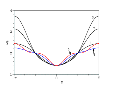
Figure 1: (Color online). The dispersion law (13) for the plane waves for $\nu=0$ (curve 1), $\nu=0.3$ (curve 2) $\nu=0.5$ (curve 3), $\nu=-0.3$ (blue curve, 4) and $\nu=-0.5$ (red curve, 5). The rest of the parameters are $\eta=0.5$ and $\kappa=1$.

The situation of the large $|\nu|$, however, does not correspond to the JJA array, because the expansion over the powers of $\nu$ obviously fails. Nevertheless, it may be relevant to other physical systems where them DDbSG equation is used. It will be discussed in the next sections.

IV Embedded soliton properties in the hamiltonian limit

In this section we consider an idealized but still very important limit of the DDbSG equation when the dissipation and the external bias are neglected ($\alpha=0$, $\gamma=0$). In this case we are interested in the existence of the traveling wave solutions that propagate with exactly the same shape and velocity:

$$\phi_{n}(t)=\phi(n-vt)\equiv\phi(z)\,\,,\,\,z\equiv n-vt\,.$$ (14)

After substituting this ansatz into the equations of motion (11) one arrives to the differential equation with delay and advance terms:

$$v^{2}\phi^{\prime\prime}(z)+\sin[\phi(z)]+\eta\sin[2\phi(z)]-$$ (15)

$$-\kappa\left\{\sum_{j=1}^{3}D_{j}(\nu)[\phi(z+j)+\phi(z-j)-2\phi(z)]\right\}=0~{},$$

which can be solved only numerically. The appropriate pseudo-spectral method has been developed in Hochstrasser et al. (1989); Eilbeck and Flesch (1990); Duncan et al. (1993) and can trace the traveling wave solution with a desired precision. Using this method we scan all possible soliton velocities from $v=0$ to $v_{max}$. The continuous DbSG equation in the dimensionless variables reads $\phi_{tt}-v_{0}^{2}\phi_{xx}+V^{\prime}(\phi)=0$, and it is Lorentz-invariant, thus $v_{max}=v_{0}$. Its discrete counterpart is not Lorentz-invariant but from the numerical simulations we have observed that a certain maximum soliton velocity exists. If the continuum approximation of Eq. (11) is performed (see the next section), one can find that the maximal kink velocity is close to its continuum counterpart $v_{max}\sim\sqrt{\kappa\sum_{j=1}^{3}j^{2}D_{j}(\nu)}$. After scanning the whole velocity interval $[0,v_{max}]$ with the pseudo-spectral method we observe the situation typical for the DNKG models Schmidt (1979); Savin et al. (2000); Flach et al. (1999); Karpan et al. (2002); Aigner et al. (2003). For all soliton velocities except some discrete set $\{{\bar{v}}_{n}\}_{n=1}^{M}$ one obtains a bound soliton-plane wave state with the non-vanishing oscillating tails. These solutions are often referred to as nanopterons Boyd (1990). The solutions that belong to the above-mentioned discrete set ($v={\bar{v}}_{n}$) are exponentially localized with the following asymptotics:

$$\phi(z)\to\left\{\begin{array}[]{cc}0\,,&z\to-\infty\\ 2\pi Q\,,&z\to+\infty\,,\end{array}\right.$$ (16)

where $Q$ is the topological charge. The set of these velocities will be called sliding velocities. As was pointed out first in Ref. Peyrard and Kruskal (1984), nanopterons or solitons with non-vanishing tails appear because for any soliton velocity $v$ there always exists a plane wave with the same phase velocity. In other words, the resonance condition

$$\omega_{L}(q)=vq,$$ (17)

always has at least one real root for any $v\neq 0$. Appearance of the ESs means that this resonance can be avoided for the selected set of velocities $\{{\bar{v}}_{n}\}_{n=1}^{M}$.

The typical dependence of the nanopteron tail amplitude $A$ on its velocity $v$ is shown in Fig. 2. Existence of the ES with ${\bar{v}}\approx 0.607$ at $\kappa=1$ and $\eta=0.5$ is clearly visible.

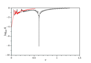
Figure 2: (Color online). Oscillation amplitude $A$ in the soliton tail as a function of its velocity for $\eta=0.5$, $\nu=-0.3$, $\kappa=1$ (black) and $\kappa=-0.45$ (red).

As it was shown for the nearest-neighbor DDbSG equation Zolotaryuk and Starodub (2015), the existence diagram for one member of the ES set has the following structure. On the parameter plane discreteness-asymmetry ($\kappa,\eta$) there exists a monotonous decaying function $\eta_{c}(\kappa)$, such that

$$\eta_{c}(\kappa)\to\left\{\begin{array}[]{cc}0\,,&\kappa\to 0\\ \infty\,,&\kappa\to+\infty\,,\end{array}\right.$$ (18)

Everywhere below this function there is no ESs and above this function there is at least one such soliton. This is quite natural because the coupling $\kappa$ should be strong enough to support the soliton propagation. Also, the parameter $\eta$ should be big enough in order to keep the system far enough from the DSG limit that is known to have no ESs. This is shown in Fig. 2 where $\kappa=0.45$ is too small to sustain an ES, but there exist an ES for $\kappa=1$.

We focus on the dependence of the ES velocity (sliding velocity) ${\bar{v}}$ on the coupling constant $\kappa$ for the fixed value $\eta$. For this purpose we construct the dependence of ${\bar{v}}$ on the renormalized coupling constant

$$\kappa^{\prime}=D_{1}(\nu)\kappa=(1+2\nu+3\nu^{2})\kappa~{}.$$ (19)

This constant should be used instead of $\kappa$ because it is the correct measure of the nearest-neighbor interaction if $\nu\neq 0$ [see Eq. (11)]. Thus, by comparing the ${\bar{v}}(\kappa^{\prime})$ for the different values of $\nu$ we find out how the next-to-nearest and second-to-nearest neighbor interaction influences the existence of embedded solitons. In Fig. 3(a) the dependence of the ES velocity on $\kappa^{\prime}$ is given. In the case of $\nu<0$ the next-neighbor interactions increase the existence range of ESs and their velocity while for $\nu>0$ the existence range together with the velocity decrease. The ${\bar{v}}(\kappa^{\prime})$ dependence is not always purely monotonic and may consist of several pieces, as for $\nu=0$ and $\nu=-0.3$

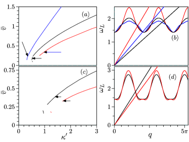
Figure 3: (Color online). Dependence of the ES velocity on the renormalized the coupling parameter $\kappa^{\prime}$ (a,c) and the roots of Eq. (17) on the dispersion laws (b,d). For all figures $\eta=0.5$. In Fig. (a) $\nu=0$ (black), $\nu=0.3$ (red), $\nu=-0.3$ (blue). In Fig. (b) the dispersion laws are shown for $\kappa=0.52$ and $\nu=0$ (black), $\nu=0.3$ (red) and $\nu=-0.3$ (blue). The solid straight lines ${\bar{v}}q$ correspond to the ES velocities pointed by the arrows in (a) and the colors correspond to the different values of $\nu$ in the same way as in (a). Figures (c) and (d) correspond to the case when $D_{3}(\nu)=0$. In Fig. (c) $\nu=0.3$ (black) and $\nu=0.4$ (red). In Fig. (d) $\kappa=0.75$ and the color of the dispersion law and the ${\bar{v}}q$ correspond to $\nu=0.3$ (black) and $\nu=0.4$ (red). The straight lines correspond to the ES velocities, pointed by the arrows in (c).

This can be easily understood from the analysis of the linear spectrum of the array. It is important to recall the result of Ref. Aigner et al. (2003) where the lowest bond of the ES velocity has been determined. This paper states that ${\bar{v}}$ cannot lie in the parameter range where the Eq. (17) has more than one root. As the velocity is decreased, the $q{\bar{v}}$ line can cross the linear spectrum band $\omega_{L}$ three, five or more times. This argument originates from the idea that the ES appears as a result of the destructive interference of the plane waves, emitted by the moving solitons. It was first formulated in Ref. Peyrard and Kruskal (1984) for the bound state of two or more $0-2\pi$ kinks in the DSG equation. In the DDbSG equation there are two limits when it turns into the standard DSG equation. The limit $\eta\to 0$ is trivial. Another limit is $\eta\to\infty$. In this case the proper renormalization of the nonlinear term is necessary (see Ref. Nishida et al. (2010)). In this limit the term $\sin 2\phi$ will dominate over the $\sin\phi$ term, and, as a result, the $0-\pi$ kinks will replace the $0-2\pi$ kinks. Thus, as was also pointed out in Ref. Bogdan et al. (2001) for the strongly dispersive continuous DbSG, in the intermediate situation with $\eta$ being large enough but finite, one can speak about the $0-2\pi$ kinks as weakly coupled pair of two $0-\pi$ kinks. Therefore, the ES for $0<\eta<\infty$ is a continuation of the two $0-\pi$ kink bound state from the limit $\eta=\infty$. Of course, if $\eta$ decreases down to the critical value $\eta_{c}$ this bound state breaks down and we have no ES. The destructive interference between these two “virtual kinks” will work only if there is just one resonance (17) to be avoided. Therefore, if the $vq$ line crosses the dispersion law more times, additional resonances appear and they cannot be suppressed.

In Fig. 3(b) this argument can be clearly demonstrated as we show how the resonance condition (17) works for the ES near the edge of its existence area. The dispersion laws corresponds to $\kappa=0.52$ in all three cases. The $\nu=0$ case is shown by the black line. The corresponding $\bar{v}(\kappa^{\prime})$ dependence is fragmented, and, apart from the main curve, has two small pieces below it. The ES velocity value, that corresponds to the black line [${\bar{v}}\approx 0.18098$, pointed by the arrow in Fig. 3(a)] creates one crossing with the dispersion law in the fourth Brillouin zone (BZ). For larger $\kappa^{\prime}$ and larger velocity the respective crossing would occur in the second BZ and that would correspond to the main curve of the $\bar{v}(\kappa^{\prime})$ dependence. Precisely this is shown by two other resonances $\nu=-0.3$ (blue curve) and $\nu=0.3$ (red curve). In these two cases the dispersion law is crossed by the respective ${\bar{v}}q$ line in the second BZ. For the $\nu=-0.3$ the the slope of the ${\bar{v}}q$ line (blue) crosses the dispersion law once but is very close to the situation when it will cross the dispersion law three times. Thus, there exists a small forbidden interval for velocities where no ES is possible. After passing this interval there is again one root of Eq. (17), but in the fourth BZ. Depending on the width of the spectrum, $\Delta\omega_{L}$, there could be single roots of Eq. (17) in the next even BZs. Therefore, we observe that positive $\nu$ plays a destructive role in the ES formation because it causes widening of the linear wave band, and, as a result, reduces the parameter space for the one-root solutions of the resonance equation (17). For the same reason, the case of $\nu<0$ is more favorable for the existence of ESs, as the linear spectrum becomes more narrow in comparison to the $\nu=0$ situation. As an interesting side observation, we note that the ES velocity always corresponds to the root of (17) that lies in the even BZ. From the plots it is quite obvious that a single root is not possible in the $3,5,\ldots,(2n+1)$th BZ. However we have not seen any ES that corresponds to the resonance in the first BZ either. We think that ES can exist only if the respective group velocity is negative because then the radiated energy travels backwards and the soliton can separate itself from it.

To study further the influence of the linear wave spectrum on the ES existence we consider the case when the dispersion law has a local maximum at $q=0$ and its minimum is placed between $q=0$ and $q=\pi$, and, in addition to that $\omega_{L}(q_{min})<\sqrt{1+2\eta}$. This can be achieved if the term $D_{2}$ in (12) dominates over the first term $D_{1}$. It should be noted that this situation can not be achieved if the expansion (8) holds. Thus, it is not directly applied to the JJ array. We put by hands $D_{3}=0$ and take $\nu=0.3$ and $\nu=0.4$. In this case the dispersion law takes the shape as in Fig. 3(d). In Fig. 3(c) we observe the further decrease of the existence area of the ES on the $\kappa$ axis. For $\nu=0.5$ we did not manage to find ES at all and for $\nu=0.6$ did not find any traveling-wave solutions of Eq. (15). This particular case is different from the dispersion laws discussed in the previous paragraphs because its lower bond decreases as $\kappa$ increases. At some point $\omega_{L}(q_{min})$ will reach zero, thus, signaling instability. This is not surprising if we think for a moment about Eq. (11) as a lattice of interacting particles and $\phi_{n}$’s as their spatial coordinates. Then the nearest-neighbor interaction term describes attractive interaction because $D_{1}(\nu)>0$ and the next-to-nearest interaction is repulsive because $D_{2}(\nu)<0$. If $\nu$ is sufficiently large, the attractive interaction is no longer strong enough to balance the repulsive term and the whole system becomes unstable. Even in the parameter range where it stays stable, the linear spectrum width becomes so big that it becomes impossible to have one root of the resonance equation (17) anywhere except the first BZ.

V Current-voltage characteristics of the annular array

Realistic simulations of the JJAs should take into account the effects of dissipation that originate from the normal electron tunneling across each junction. Also, the external DC bias should be included into consideration. Thus, the full Eqs. (11) should be solved with $\alpha>0$ and $\gamma\neq 0$.

V.1 Continuous approximation

In the continuous approximation the DDbSG equation can be written as a standard double sine-Gordon (DbSG) equation:

$$\phi_{tt}-v_{0}^{2}\phi_{xx}+\sin\phi+\eta\sin{2\phi}=-\alpha\phi_{t}+\gamma~{},$$ (20)

$$v_{0}^{2}=\kappa\sum_{j=1}^{3}j^{2}D_{j}(\nu)~{}.$$

In order to get the current-voltage characteristics (CVCs) in this case we use the energy balance approach, developed previously McLaughlin and Scott (1978). According to this approach the total power $\bar{V}\gamma$, applied to the soliton is compensated by the dissipation, $\bar{V}_{c}\gamma=-P_{diss}$. The dissipative losses can be easily computed if we use the exact solution Campbell et al. (1986); Condat et al. (1983) of the unperturbed continuous DbSG equation with the arbitrary velocity $v$:

$$P_{diss}=-\alpha\int_{-\infty}^{+\infty}\phi_{t}^{2}dx=\frac{4\alpha\Phi(\eta)}{\pi\sqrt{v_{0}^{2}-v^{2}}},$$ (21)

$$\Phi(\eta)=\frac{\sqrt{1+2\eta}}{2}\left[1+\right.$$

$$\left.+\frac{1}{\sqrt{2\eta(2\eta+1)}}~{}\mbox{arctanh}\sqrt{\frac{2\eta}{1+2\eta}}\right]~{},$$ (22)

As a result we arrive to the analytical expression for the average voltage drop:

$$\bar{V}_{c}=\frac{2\pi v}{N}=\frac{2\pi v_{0}}{N}\left[1+\Phi^{2}(\eta)\left({4\alpha}\over{\pi\gamma}\right)^{2}\right]^{-1/2}~{}.$$ (23)

In the limit $\eta\to 0$ the standard SG equation is restored. From Eq. (V.1) one observes that $\Phi(\eta)_{\eta\to 0}\to 1$. Thus, the equilibrium velocity coincides with the equilibrium velocity of the SG equation $v=\left[1+\left({4\alpha}\over{\pi\gamma}\right)^{2}\right]^{-1/2}$ McLaughlin and Scott (1978).

V.2 Numerically computed current-voltage characteristics

The CVCs provide the necessary information about the JJ array dynamics and are accessible through experimental measurements. The average voltage drop is defined as

$${\bar{V}}=\frac{1}{N}\sum_{n=1}^{N}\lim_{t\rightarrow\infty}\frac{1}{t}\int_{0}^{t}{\dot{\phi}}_{n}(t^{\prime})dt^{\prime}~{}.$$ (24)

If there is a soliton that moves along the array with velocity $v$ it will produce the average voltage drop $2\pi v/N$. Since Eq. (11) is dissipative, we are going to deal with its attractor solutions. The numerically computed CVC curves are shown in Fig. 4. To obtain these figures we have changed the bias current $\gamma$ in both directions: from $\gamma=0$ till $\gamma=0.06$ and in the reverse way. To integrate Eqs. (11) the 4th order Runge-Kutta method was used.

We remind here the basic difference between the CVCs in the continuous JJs and in the JJ arrays. In the former case the CVC is a continuous monotonic function given by Eq. (23). The soliton dynamics in the continuous JJ is qualitatively similar to the particle moving in the viscous liquid under the influence of gravitation, where the DC bias plays the role of gravitation and $\alpha$ plays the role of viscosity. Discreteness and periodic boundary conditions bring the fundamental changes to the shape of the CVCs. In the JJ array they constitute a series of separate curves, as can be seen in Fig. 4. The presence of the periodic boundary conditions means that only a certain integer number of the plane wave periods can fit into the array of $N$ junctions Ustinov et al. (1993); Braun et al. (2000). Each branch corresponds to the distinct number of periods and the wavelength of each period is defined by the resonance condition (17). Sometimes it is not possible to identify separate branches, especially for the large values of $\gamma$, because the JJA dynamics may be quasiperiodic or even chaotic. The continuous CVCs (23) are given by the solid lines. It appears that this approximation is in satisfactory agreement with the numerical data only near the origin of the CVC. Another prominent signature of discreteness is hysteresis of the CVCs. If we start from the superconducting state (pinned soliton), it will stay pinned until the bias $\gamma$ reaches the critical value. This critical value depends only on the static properties of the array and does not depend on dissipation. The retrapping current is the minimal current for which soliton motion is possible. This current decreases with the decrease of $\alpha$.

The case when no ESs exist in the hamiltonian limit is presented in Fig. 4(a). One can observe that the CVCs occupy almost all accessible voltage range. For $\kappa=0.5$ the CVC is approximately continuous for the larger voltages, while for the smaller voltages some vertical branches can be identified. Closer to the origin the separate branches can hardly be distinguished from each other. For $\kappa=0.8$ the vertical branches appear more clearly because for the larger values of $\kappa$ the JJ dynamics is less chaotic. The behavior near the origin is similar to the $\kappa=0.5$ case.

Figure 4: (Color online). Current-voltage characteristics for the annular JJA with $N=30$ junctions. Figure (a) corresponds to $\kappa=0.5$, $\nu=\eta=0$ (red $\circ$) and $\eta=0.1$, $\kappa=0.8$ (black $\blacklozenge$). In both cases $\alpha=0.02$ and $\nu=0$. Continuous approximation is shown by the solid black lines. Figure (b) corresponds to $\kappa=0.8$, $\eta=0.5$, $\nu=-0.3$, $\alpha=0.02$ (black $\blacklozenge$) and $\alpha=0.01$ (red $\circ$). Inset shows the Josephson phase distribution for $\gamma=0.01$ ($\circ$) and $\gamma=0.0079$ ($\blacklozenge$). Vertical blue line corresponds to the voltage $V=2\pi{\bar{v}}/N$, where ${\bar{v}}$ is the ES velocity (see text for details).

The best manifestation of the ESs is possible if the parameter $\eta$ is large enough to keep the system far from the DSG limit. In Fig. 4(b) the case of $\eta=0.5$ is considered. On the respective CVC one observes the situation similar to the previously discussed case of the DDbSG model with just the nearest neighbour interactions ($\nu=0$) Zolotaryuk and Starodub (2015). The general picture looks more ordered with the distinct separate almost vertical CVC branches that exist only above some certain value of ${\bar{V}}$. The inaccessible voltage interval (IVI) $[0,V_{IVI}]$ is formed, within which there is no CVC branches. The upper edge of this range appears to lie close to the voltage, produced by the ES in the hamiltonian limit, which is ${\bar{V}}=2\pi{\bar{v}}/N\approx 0.0969$ and is shown in the figure by the vertical blue line. For the respective system parameters ($\eta=0.5$, $\nu=-0.3$) the upper bond of the IVI is $V_{IVI}\approx 0.086$, and it weakly depends on dissipation (up to the fourth decimal for $\alpha=0.01$ and $\alpha=0.02$). From Fig. 4 we see that not the lowest but the third lowest branch of CVC springs off the voltage $2\pi{\bar{v}}/N$ that corresponds to the ES in the hamiltonian limit. The threshold value of the DC bias at the voltage $V_{IVI}$ decreases as $\alpha$ tends to zero, what is a principal difference from the situation when no ESs is possible. The soliton profile at the edge of the IVI has very small radiating tails [see the inset of Fig. 4(b)] while the soliton profile from the neighboring branch of the CVC has much better pronounced oscillating asymptotics. We have computed the detuning $\epsilon=2\pi{\bar{v}}/N-V_{IVI}$ of the IVI edge from the voltage created by the moving ES. This detuning parameter is given in Tab. 1 for the parameters of Fig. 4 except $\nu$ which is increased up to $\nu=0$.

$\nu$	$\epsilon$
-0.3	0.0109
-0.2	0.0063
-0.1	0.0045
-0.05	0.0047
0	0.0008

Table 1: The detuning parameter $\epsilon=2\pi{\bar{v}}/N-V_{IVI}$ as a function of $\nu$. The other parameters are as in Fig.4

As we approach to the pure next-neighbor limit ($\nu$), the difference between the upper edge of IVI and the voltage, produced by the moving ES becomes very small. We conclude that in the presence of small dissipation and for the small values of DC bias $\gamma$ the JJA dynamics settles on the attractor that originates from the ES soliton in the hamiltonian limit.

VI Discussion and conclusions

In this paper we have investigated how the presence of the next-to-nearest and second-to-nearest interactions in the nonlinear discrete Klein-Gordon (NDKG) lattice influences the properties of the embedded solitons (ES). We have taken the discrete double sine-Gordon equation as a working model because of the broad range of its application in various fields of modern physics and because it is known to support ESs in the limit of the nearest-neighbor interactions Zolotaryuk and Starodub (2015). In particular, this equation is used for modeling of the arrays of JJs, in particular arrays of SFS or SIFS junctions Goldobin et al. (2007). The appearance of the next-to-nearest and second-to-nearest interactions is due to the fact that the inductive coupling between the neighboring cells of the array was taken into account. If this coupling is weak comparing to the self-inductance of the cell, the resulting equations of motion for the Josephson phase can be rewritten as the DDbSG equation with the next-neighbor and second-neighbor interactions. The interaction with the $j$th neighbor comes as a discrete Laplasian term with the coefficient of the order ${\cal O}(\nu^{j-1})$, where $\nu$ is the ratio of the mutual inductance between the neighboring cells of the array to the self-inductance of the cell.

We have demonstrated that existence of embedded solitons (ESs) depends primarily on the properties of the spectrum of the linear waves of the system. Our results confirm previous findings Aigner et al. (2003) where it was shown that a discrete ES cannot exist with velocities for which Eq. (17) has more than one root. The case of $\nu<0$ is more relevant to the JJ physics and for it the next-to-nearest and the second-to-nearest interactions create more favorable conditions for the ESs formation as compared to the $\nu=0$ limit. In particular, the existence range (in the terms of the nearest-neighbor interaction term) for the ESs on the increases, the ES velocity increases as well. For the positive values of $\nu$ the situation is opposite. The ES velocity decreases, as well as the existence range. The explanation is as follows: in the former case the linear wave spectrum narrows, thus creating more possibilities for having just one root of the resonance condition (17). In the latter case the linear band widens and, as a result, makes more difficult to have just one root of this equation.

This research can be further extended into other physical models that are not connected to the Josephson effect. Recent research on the nonlinear electric circuits with the next-neighbor interactions Chen et al. (2018) seems to be a promising field for application of the ideas developed in this article.

References

- Condat et al. (1983) C. A. Condat, R. A. Guyer, and M. D. Miller, Phys. Rev. B 27, 474 (1983).
- Campbell et al. (1986) D. K. Campbell, M. Peyrard, and P. Sodano, Physica D 19, 165 (1986).
- Dodd et al. (1975) R. K. Dodd, R. K. Bullough, and S. Duckworth, Journal of Physics A: Mathematical and General 8, L64 (1975).
- Maki and Kumar (1976) K. Maki and P. Kumar, Phys. Rev. B 14, 118 (1976).
- Remoissenet (1981) M. Remoissenet, Journal of Physics C: Solid State Physics 14, L335 (1981).
- Peyrard and Remoissenet (1982) M. Peyrard and M. Remoissenet, Phys. Rev. B 26, 2886 (1982).
- Braun et al. (1990) O. M. Braun, Y. S. Kivshar, and I. I. Zelenskaya, Phys. Rev. B 41, 7118 (1990).
- Goldobin et al. (2007) E. Goldobin, D. Koelle, R. Kleiner, and A. Buzdin, Phys. Rev. B 76, 224523 (2007).
- Atanasova et al. (2010) P. K. H. Atanasova, T. L. Boyadjiev, Y. U. M. Shukrinov, E. V. Zemlyanaya, and P. Seidel, Journal of Physics Conference Series 248 (2010).
- Golubov et al. (2004) A. A. Golubov, M. Y. Kupriyanov, and E. Il’ichev, Rev. Mod. Phys. 76, 411 (2004).
- Askerzade (2015) I. N. Askerzade, Low Temp. Phys. 41, 241 (2015).
- Alfimov et al. (2014a) G. Alfimov, A. Malishevskii, and E. Medvedeva, Physica D: Nonlinear Phenomena 282, 16 (2014a), ISSN 0167-2789.
- Nishida et al. (2010) M. Nishida, T. Kanayama, T. Nakajo, T. Fujii, and N. Hatakenaka, Physica C 470, 832 (2010).
- Barone and Paterno (1982) A. Barone and G. Paterno, Physics and Applications of the Josephson Effect (Wiley, New York, 1982).
- Ustinov (1998) A. V. Ustinov, Physica D 123, 315 (1998).
- Zolotaryuk and Starodub (2015) Y. Zolotaryuk and I. O. Starodub, Phys. Rev. E 91, 013202 (2015).
- Champneys et al. (2001) A. Champneys, B. Malomed, J. Yang, and D. Kaup, Physica D 152-153, 340 (2001).
- Peyrard and Kruskal (1984) M. Peyrard and M. D. Kruskal, Physica D 14, 88 (1984).
- Boyd (1990) J. P. Boyd, Nonlinearity 3, 177 (1990).
- Aigner et al. (2003) A. Aigner, A. Champneys, and V. Rothos, Physica D 186, 148 (2003).
- Friesecke and Wattis (1994) G. Friesecke and J. A. D. Wattis, Commun. Math. Phys. 161, 391 (1994).
- Schmidt (1979) V. H. Schmidt, Phys. Rev. B 20, 4397 (1979).
- Flach et al. (1999) S. Flach, Y. Zolotaryuk, and K. Kladko, Phys. Rev. E 59, 6105 (1999).
- Barashenkov et al. (2005) I. V. Barashenkov, O. F. Oxtoby, and D. E. Pelinovsky, Phys. Rev. E 72, 035602(R) (2005).
- Oxtoby et al. (2006) O. Oxtoby, D. E. Pelinovsky, and I. V. Barashenkov, Nonlinearity 19, 217 (2006).
- Alfimov et al. (2014b) G. L. Alfimov, E. Medvedeva, and D. E. Pelinovsky, Phys. Rev. Lett. 112, 054103 (2014b).
- Zolotaryuk et al. (1997) Y. Zolotaryuk, J. C. Eilbeck, and A. V. Savin, Physica D 108, 81 (1997).
- Savin et al. (2000) A. V. Savin, Y. Zolotaryuk, and J. C. Eilbeck, Physica D 138, 265 (2000).
- Karpan et al. (2002) V. M. Karpan, Y. Zolotaryuk, P. L. Christiansen, and A. V. Zolotaryuk, Phys. Rev. E 66, 066603 (2002).
- Dmitriev et al. (2008) S. V. Dmitriev, A. Khare, P. G. Kevrekidis, A. Saxena, and L. Hadžievski, Phys. Rev. E 77, 056603 (2008).
- Archilla et al. (2013) J. F. R. Archilla, Y. A. Kosevich, N. Jimenez, V. J. Sanchez-Morcillo, and L. M. Garcia-Raffi, Ukr. J. Phys. 58, 646-656 (2013); J. F. R. Archilla, Y. Zolotaryuk, Y. A. Kosevich, and Y. Doi, Chaos: An Interdisciplinary Journal of Nonlinear Science 28, 083119 (2018).
- Pfeiffer et al. (2006) J. Pfeiffer, M. Schuster, J. A. A. Abdumalikov, and A. V. Ustinov, Phys. Rev. Lett. 96, 034103(4) (2006).
- Gaididei et al. (1995) Y. Gaididei, N. Flytzanis, A. Neuper, and F. G. Mertens, Phys. Rev. Lett. 75, 2240 (1995).
- Szameit et al. (2009) A. Szameit, R. Keil, F. Dreisow, M. Heinrich, T. Pertsch, S. Nolte, and A. Tünnermann, Opt. Lett. 34, 2838 (2009).
- Chen et al. (2018) X.-L. Chen, S. Abdoulkary, P. G. Kevrekidis, and L. Q. English, Phys. Rev. E 98 (2018).
- Phillips et al. (1993) J. R. Phillips, H. S. J. van der Zant, J. White, and T. P. Orlando, Phys. Rev. B 47, 5219 (1993).
- Watanabe et al. (1996) S. Watanabe, H. S. J. van der Zant, S. H. Strogatz, and T. P. Orlando, Physica D 97, 429 (1996).
- Domínguez and José (1996) D. Domínguez and J. V. José, Phys. Rev. B 53, 11692 (1996).
- Mazo (1996) J. J. Mazo, J. J. Ciria, Phys. Rev. B 54,16068 (1996).
- Filatrella et al. (1999) G. Filatrella, A. Petraglia, and G. Rotoli, Eur. Phys. J. B 12, 23 (1999).
- Gray (2006) R. M. Gray, Toeplitz and Circulant Matrices: A Review, vol. 2 of Foundation and Trends in Communications and Information Theory (NOW Publishers Inc., Boston-Delft, 2006).
- Hochstrasser et al. (1989) D. Hochstrasser, F. Mertens, and H. Büttner, Physica D: Nonlinear Phenomena 35, 259 (1989).
- Eilbeck and Flesch (1990) J. C. Eilbeck and R. Flesch, Phys. Lett. A 149, 200 (1990).
- Duncan et al. (1993) D. Duncan, J. Eilbeck, H. Feddersen, and J. Wattis, Physica D 68, 1 (1993).
- Bogdan et al. (2001) M. M. Bogdan, A. Kosevich, and G. A. Maugin, Wave Motion 34, 1 (2001).
- McLaughlin and Scott (1978) D. W. McLaughlin and A. C. Scott, Phys. Rev. A 18, 1652 (1978).
- Ustinov et al. (1993) A. V. Ustinov, M. Cirillo, and B. A. Malomed, Phys. Rev. B 47, 8357 (1993).
- Braun et al. (2000) O. Braun, B. Hu, and A. Zeltser, Phys. Rev. E 62, 4235 (2000).