IFJPAN-IV-2018-20

Machine learning classification: case of

Higgs boson CP state in $H\to\tau\tau$ decay at LHC

K. Lasocha^a,b, E. Richter-Was^a, D. Tracz^a,∗, Z. Was^c and P. Winkowska^d,∗
a Institute of Physics, Jagellonian University, ul. Lojasiewicza 11, 30-348 Kraków, Poland

^b CERN, 1211 Geneva 23, Switzerland

^c IFJ-PAN, 31-342, ul. Radzikowskiego 152, Kraków, Poland
^d Department of Computer Science, AGH USiT, Al. Mickiewicza 30, 30-059 Kraków, Poland

ABSTRACT

Machine Learning (ML) techniques are rapidly finding a place among the methods of High Energy Physics data analysis. Different approaches are explored concerning how much effort should be put into building high-level variables based on physics insight into the problem, and when it is enough to rely on low-level ones, allowing ML methods to find patterns without explicit physics model.

In this paper we continue the discussion of previous publications on the CP state of the Higgs boson measurement of the $H\to\tau\tau$ decay channel with the consecutive $\tau^{\pm}\to\rho^{\pm}\nu$; $\rho^{\pm}\to\pi^{\pm}\pi^{0}$ and $\tau^{\pm}\to a_{1}^{\pm}\nu$; $a_{1}^{\pm}\to\rho^{0}\pi^{\pm}\to 3\pi^{\pm}$ cascade decays. The discrimination of the Higgs boson CP state is studied as a binary classification problem between CP-even (scalar) and CP-odd (pseudoscalar), using Deep Neural Network (DNN). Improvements on the classification from the constraints on directly non-measurable outgoing neutrinos are discussed. We find, that once added, they enhance the sensitivity sizably, even if only imperfect information is provided. In addition to DNN we also evaluate and compare other ML methods: Boosted Trees (BT), Random Forest (RF) and Support Vector Machine (SVN).

IFJPAN-IV-2018-20 December 2018

^(∗) In time of working on this project.

This project was supported in part from funds of Polish National Science Centre under decisions DEC-2017/27/B/ST2/01391. DT and PW were supported from funds of Polish National Science Centre under decisions DEC-2014/15/B/ST2/00049.

Majority of the numerical calculations were performed at the PLGrid Infrastructure of the Academic Computer Centre CYFRONET AGH in Krakow, Poland.

1 Introduction

Machine Learning (ML) techniques find increasing number of applications in High Energy Physics phenomenology. With Tevatron and the LHC experiments, it became an analysis standard. The ML techniques are used for event selection, event classification, background suppression for the signal events of the interest, etc. For a comprehensive recent review see [1, 2, 3]. Over the last years the most significant progress in phenomenology due to ML techniques, in particular recent development in neural network methods, was in hadronic jets reconstruction and classification: jet substructure, jet-flavour, jet-charge and jet-mass. They addressed successfully long-standing challenges of more classical algorithms, see e.g. Refs. [4, 5, 6, 7, 8, 9, 10].

In this paper we present studies on the seemingly related problem: exploration how the substructure and pattern of hadronically decaying $\tau$ leptons can be useful to determine the CP state of the Higgs boson in the decay $H\to\tau\tau$. Theoretical description of the process incuding $\tau$ lepton decays is relatively simple and of the minor theoretical ambiguities only. On the other hand, complicated detection approach remains a challenge. For example, indirect constraints had to be devised and validated instead of non-measurable $\tau$-neutrino momenta. Related part of the sensitivity was often compromised.

This problem has a long history [11, 12]. It was studied both for electron-positron [13, 14] and for hadron-hadron [15, 16] colliders. Despite some interest, CP in $H\to\tau\tau$ was not measured or even explored in LHC analysis designs. While more classical experimental analysis strategies have been prepared and documented, see e.g. [17], for HL-LHC strategies exploring the ML methods are still at the early stage.

A typical experimental data sample consists of events. Each event can be understood as a point in a multi-dimensional coordinate space, representing four-momenta and flavours of observed particles or groups of particles. The physics goal is to identify properties of distributions constructed from these events and to interpret them in physically meaningful way. The ML algorithms with only the low-level features of the event are not necessarily able to capture efficiently all information available. The best performing strategy still seems to be mixing of low-level information with the human-derived high-level features, based on the physics insight into the problem. Examples of such analyses are presented in [18, 19]. The strategy of mixing low-level and high-level features, prepared to remove trivial (physics-wise) symmetries are explored successfully there. Then, the ML algorithms do not need to learn some basic physics rules, like rotation symmetry.

In the previous papers [20, 21] we have demonstrated that ML methods, like Deep Neural Network (DNN) [22], can serve as a promising analysis method to constrain the Higgs boson CP state in the decay channel $H\to\tau\tau$. We considered two decay modes of the $\tau$ leptons: $\tau^{\pm}\to\rho^{\pm}\nu$, $\tau^{\pm}\to a_{1}^{\pm}\nu$, followed by $\rho^{\pm}\to\pi^{\pm}\pi^{0}$ and $a_{1}^{\pm}\to\rho^{0}\pi^{\pm}\to 3\ \pi^{\pm}$. This forms three possible hadronic final state configurations: $\rho^{\pm}\rho^{\mp}$, $a_{1}^{\pm}\rho^{\mp}$ and $a_{1}^{\pm}a_{1}^{\mp}$, each accompanied by the $\tau$-neutrino pair. The information about the Higgs boson CP state is encoded in the angles between outgoing decay products and angles between intermediate resonances decay planes. From the early studies [12, 23] performed with the rather classical optimal variable  approach, we have observed that the best discrimination was achievable from features constructed in the rest-frame of the primary intermediate resonance pair of the $\tau$ decays, with the $z$-axis aligned to these resonances direction. This idea was explored also in [20] and will be followed in this paper. We have investigated inputs consisting of mixed low-level and high-level features. Many of the high-level features turned out to be not necessary, but nevertheless provided benchmark results. On the other hand, (post-fact seemingly simple) non-trivial choices for the representation of some low-level features was necessary to achieve any significant result.

The studies presented in paper [20] were limited to input from the hadronic decay products, $\pi^{\pm},\pi^{0}$; no detector effects were taken into account. That study was followed by a more systematic evaluation within the context of experimental analysis [21], namely applying simplified detector effects to the input features. The conclusions of [20] on the DNN method performance survived, and we will not follow this evaluation in the scope of the paper again.

Studies presented in [20] have shown, that the case of $\rho^{\pm}\rho^{\mp}$ followed by $a_{1}^{\pm}\rho^{\mp}$ is the most sensitive to Higgs CP channel, and somewhat weaker sensitivity is achieved in $a_{1}^{\pm}a_{1}^{\mp}$ case. Should all the decay channels be equally sensitive to the Higgs CP state? In [24] it was demonstrated that yes, the sensitivity of each $\tau$ decay channel to spin is the same. Unfortunately, this requires control of all $\tau$ decay products momenta, in particular of non-measurable neutrinos. Studies presented in [20] did not rely on the complete information, limiting input information to the hadronic (visible) decay products only. However, it is possible to overcome this limitation and reconstruct, with approximation, the neutrino momenta from the $\tau$ decay vertex position and event kinematics (momenta of visible $\tau$ decay products, overall missing $p_{T}$ and overall collision center of mass system energy). Such reconstruction is challenging from the experimental perspective and also for the analysis design: relations between necessary features are more complicated. Nevertheless this brings new opportunities for ML methods which we will explore with the help of expert variables: the azimuthal angles of the neutrino orientation. The encouragement that the angle may become experimentally available with adequate precision can be concluded from a recent experimental publication of the LHC collaborations on the $H\to\tau\tau$ signal measurement [25, 26], $\tau$ substructure reconstruction and classification [27, 28] and also progress on the precision of B meson decay vertex position measurements  [29, 30].

We attempt to reconstruct the two neutrinos four-momenta (i.e. 6 quantities) from the experimentally available quantities and examine when such approximate information can be useful. To achieve this goal the following 3 steps are proposed:

1. reconstruction of neutrino 4-momenta components collinear to directions of visible decay products of $\tau$ leptons, from the whole event missing transverse energy $E^{x}_{miss},E^{y}_{miss}$ and from the invariant mass of the Higgs boson $m_{H}$,

2. reconstruction of the transverse part of neutrino momenta from the $\tau$ lepton invariant mass constraint,

3. reconstruction of the two remaining azimuthal angles $\phi_{\nu_{1}}$, $\phi_{\nu_{2}}$ of the neutrinos (or equivalent information); with the help of $\tau$-decay position vertices.

After step (1) we have 4 independent variables to constrain, after step (2) only two remain. The load on constraints from the $\tau$ decay vertex position, probably the least precise to measure, is minimized. This approach can be understood as an attempt to construct high-level feature with the expert-supported design. This, if useful, may be later replaced with better choices. Several papers with optimal variables in mind followed such strategy [13, 14, 16].

For compatibility, we use the same simulated samples as for Ref. [20], namely Monte Carlo events of the Standard Model, 125 GeV Higgs boson, produced in pp collision at 13 TeV centre-of-mass energy, generated with Pythia 8.2 [31] and with spin correlations simulated using TauSpinner [23]. For $\tau$ lepton decays we use Tauolapp [32]. All spin and parity effects are implemented with the help of TauSpinner weight $wt$. That is why the samples prepared for the CP even or odd Higgs are correlated. For each channel we use about $10^{7}$ simulated Higgs events . To partly emulate detector conditions, a minimal set of cuts is used. We require that the transverse momenta of the visible decay products combined, for each $\tau$, are larger than 20 GeV. It is also required that the transverse momentum of each $\pi^{\pm}$ is larger than 1 GeV.

As in [20] we perform DNN analysis for the three channels of the Higgs i.e. $\tau$ lepton-pair decays, denoted respectively as: $\rho^{\pm}-\rho^{\mp}$, $a_{1}^{\pm}-\rho^{\mp}$ and $a_{1}^{\pm}-a_{1}^{\mp}$. Only two hypotheses on Higgs parity are confronted. However, extension to parametrised classification, similar to the approach taken in  [33], could be envisaged as an obvious next step; the measurement of the Higgs CP parity mixing angle. Our paper can be also understood as a work in that direction.

Our baseline for ML methods is the DNN, nonetheless we have also worked with more classical ML techniques like Boosted Trees (BT) [34], Random Forest (RF) [35] and Support Vector Machine (SVM) [36]. The comparative analysis is presented for the $\rho^{\pm}-\rho^{\mp}$ case and for smaller events samples of about $10^{6}$ events.

Our paper is organized as follows. In Section 2 we briefly recall the physics nature of the problem and results from previous studies of Ref. [20]. In Section 3 we discuss how to reconstruct, with some approximation, the outgoing neutrinos momenta. We exploit: collinear approximation, mass constraints, and information on spatial position of production and decay vertices. In Section 4 we present an improvement in the DNN classification from information on the neutrinos. We quantify what is the necessary precision on neutrinos azimuthal angle to improve the performance of the classifier. In Section 5 the main results are sumarised and outlook is provided.

In Appendix A details concerning the DNN analysis implementation are given. In Appendix B results achieved on the problem, but with other ML techniques: – BDT, RF and SVM – are presented. We also discuss technical performance, like usage of CPU or transient memory.

2 Classification based on hadronic decay products

Let us comment briefly on a few selected results  from paper [20], summarized in Table 1. For the DNN classification, only directly measurable 4-momenta of the hadronic decay products of the $\tau$ leptons were considered. They were boosted to the rest-frame of the primary intermediate resonance pairs; respectively $\rho^{\pm}-\rho^{\mp}$, $a_{1}^{\pm}-\rho^{\mp}$ or $a_{1}^{\pm}-a_{1}^{\mp}$. All four vectors were later rotated to the frame where primary resonances were placed along the $z$-axis. It greatly improved the learning process. The DNN algorithm did not have to e.g. rediscover rotational symmetry and from the very beginning internal weights of the DNN algorithms could determine transverse CP sensitive degrees of freedom from the longitudinal ones. To quantify the performance for Higgs CP classification we have used a weighted Area Under Curve (AUC) and Receiver Operator Characteristic (ROC) curve [37, 38]. For each simulated event we know, from the calculated matrix elements, the probability that an event is sampled as scalar or pseudoscalar (for details see Appendix A). This forms so called oracle predictions, i.e. ultimate discrimination for the problem which is about 0.782, independently  of the $\tau$ decay channels. Random classification corresponds to 0.500.

For the studied $\tau$-pair decay channels, the AUC in the 0.557 - 0.638 range was achieved. Note, that so much lower than oracle predictions AUC is due to missing information on the neutrino momenta, which are important carriers of the spin information, but are not accessible directly from the measurement. Let us explain very briefly the physics context of the problem.

The Higgs boson Yukawa coupling expressed with the help of the scalar–pseudoscalar parity mixing angle $\phi$ reads as

$${\cal L}_{Y}=N\;\bar{\tau}{\mathrm{h}}(\cos\phi+i\sin\phi\gamma_{5})\tau$$ (1)

where $N$ denotes normalization, $\mathrm{h}$ Higgs field and $\bar{\tau}$, $\tau$ spinors of the $\tau^{+}$ and $\tau^{-}$. The matrix element squared for the scalar / pseudoscalar / mix parity Higgs, with decay into $\tau^{+}\tau^{-}$ pairs can be expressed as

$$|M|^{2}\sim 1+h_{+}^{i}\;h_{-}^{j}\;R_{i,j};\;\;\;\;\;i,j=\{x,y,z\}$$ (2)

where $h_{\pm}$ denote polarimetric vectors of $\tau$ decays (solely defined by $\tau$ decay matrix elements) and $R_{i,j}$ the density matrix of the $\tau$ lepton pair spin state. In Ref. [40] details of the frames used for the definition of $R_{i,j}$ and $h_{\pm}$ are given. The corresponding CP sensitive spin weight $wt$ is simple:

$$wt=1-h_{{+}}^{z}h_{{-}}^{z}+h_{{+}}^{\perp}R(2\phi)~{}h_{{-}}^{\perp}.$$ (3)

The formula is valid for $h_{\pm}$ defined in $\tau^{\pm}$ rest-frames, $h^{z}$ stands for longitudinal and $h^{\perp}$ for transverse component of $h$. $R(2\phi)$ denotes the matrix of $2\phi$ angle rotation around the $z$ direction: $R_{xx}=R_{yy}={\cos 2\phi}$, $R_{xy}=-R_{yx}={\sin 2\phi}$. The $\tau^{\pm}$ decay polarimetric vectors $h_{+}^{i}$, $h_{-}^{j}$, in the simplest case of $\tau^{\pm}\to\pi^{\pm}\pi^{0}\nu$ decay, read

$$h^{i}_{\pm}={\cal N}\Bigl{(}2(q\cdot p_{\nu})q^{i}-q^{2}p_{\nu}^{i}\Bigr{)},\;\;\;$$ (4)

where $\tau$ decay products $\pi^{\pm}$, $\pi^{0}$ and $\nu_{\tau}$ 4-momenta are denoted respectively as $p_{\pi^{\pm}}$, $p_{\pi^{0}},p_{\nu}$ and $q=p_{\pi^{\pm}}-p_{\pi^{0}}$. For $h_{\pm}^{i}$ of $\tau^{\pm}\to\pi^{\pm}\pi^{\pm}\pi^{\mp}\nu$ the formula is longer, because dependence on modeling of the decay appear too [21]. Obviously, complete CP sensitivity can be extracted only if $p_{\nu}$ is known. Note that the spin weight $wt$ is a simple first order trigonometric polynomial in a (doubled) Higgs CP parity mixing angle. This observation is valid for all $\tau$ decay channels.

Table 1: The DNN performance taken from [20] for discrimination between scalar and pseudoscalar Higgs CP state. For DNN classification only hadronic decay products 4-momenta are used.

Line content	Channel: $\rho^{\pm}-\rho^{\mp}$	Channel: $a_{1}^{\pm}-\rho^{\mp}$	Channel: $a_{1}^{\pm}-a_{1}^{\mp}$
	$\rho^{\pm}\to\pi^{\pm}\pi^{0}$	$a_{1}^{\pm}\to\rho^{0}\pi^{\pm},\rho^{0}\to\pi^{+}\pi^{-}$	$a_{1}^{\pm}\to\rho^{0}\pi^{\pm},\rho^{0}\to\pi^{+}\pi^{-}$
		$\rho^{0}\to\pi^{+}\pi^{-}$
Fraction of $H\to\tau\tau$	6.5%	4.6%	0.8%
Number of features	24	32	48
Oracle predictions	0.782	0.782	0.782
DNN classification (AUC)	0.638	0.590	0.557

3 Approximating components of neutrino momenta

Our conjecture is that some of the steps listed in the introduction and presented below may in the future be replaced or optimized with the solutions present in ML libraries. The expert variables, in particular $\phi_{\nu_{1}}$, $\phi_{\nu_{2}}$, will not be needed. We need to explain our construction in detail first.

We start with approximate neutrino momenta in the ultra-relativistic (collinear) approximation. We temporarily assume that neutrino momenta and visible $\tau$ products momenta are collinear to each other. Later we relax this oversimplification. This gives a reasonable approximation for collinear components which are the largest ones (not only in the laboratory frame but also in the Higgs rest-frame and the rest-frame of its visible decay products).

3.1 Collinear approximation

The basic kinematical constraint on 4-momenta of each $\tau^{\pm}\to had^{\pm}\;\nu$ decay reads ( $had^{\pm}$ stands for the hadronic system produced in decay, i.e. $\pi^{\pm},\pi^{0}$, etc. combined):

$$p_{\tau_{1}}=\ \ p_{{had}_{1}}+p_{\nu_{1}},\ \ \ \ \ \ \ p_{\tau_{2}}=\ \ p_{{had}_{2}}+p_{\nu_{2}}$$ (5)

where $p_{\tau_{1}},p_{\tau_{2}}$ denote 4-momenta of decaying $\tau$ leptons; $p_{{had}_{1}},p_{{had}_{2}}$ denote 4-momenta of their hadronic (i.e. measurable) decay products combined and $p_{\nu_{1}},p_{\nu_{2}}$ denote 4-momenta of the decay neutrinos.

We temporarily assume that the directions of the hadronic decay products and neutrino are parallel to the direction of the decaying $\tau$ and

$$\vec{p}_{had}=\ \ x\cdot\vec{p}_{\tau},\ \ \ \ \ \ \ \vec{p}_{\nu}=\ \ (1-x)\cdot\vec{p}_{\tau},$$ (6)

where $x$ is of the (0,1) range, then for the $\tau^{+}$ and $\tau^{-}$ we can write:

$$\vec{p}_{\nu}=\ \ \frac{1-x}{x}\cdot\vec{p}_{had}=\ \ \alpha\cdot\vec{p}_{had}.$$ (7)

From Eq. (7) we obtain

$$|\vec{p}_{\nu_{1}}|=\ \ \alpha_{1}\cdot|\vec{p}_{{had}_{1}}|,\ \ \ \ \ \ \ |\vec{p}_{\nu_{2}}|=\ \ \alpha_{2}\cdot|\vec{p}_{{had}_{2}}|.$$ (8)

These relations hold in the laboratory frame and in the rest-frame of the hadronic decay products as well, which is a consequence of properties of Lorentz transformations of ultra-relativistic particles. That is why we can calculate $\alpha_{1}$, $\alpha_{2}$ in the laboratory frame but use them in the rest-frame of the hadronic decay products combined. That frame seems to be optimal [20] for the construction of expert variables for ML classification.

3.1.1 The $E^{x}_{miss},E^{y}_{miss}$ constraints

The laboratory frame event momentum imbalance in the plane transverse to the beam direction, usually denoted as $E_{miss}^{x},E_{miss}^{y}$, can be used to constrain neutrino momenta. It can be attributed to the sum of transverse components of the neutrino momenta, but it also accumulates all imperfections of the reconstruction of the other outgoing particles of that event. Then, thanks to relation (7):

$$E_{miss}^{x} =\ \ p_{\nu_{1}}^{x}+p_{\nu_{2}}^{x}=\ \ \alpha_{1}\cdot p_{{had}_{1}}^{x}+\alpha_{2}\cdot p_{{had}_{2}}^{x},$$ (9)

$$E_{miss}^{y} =\ \ p_{\nu_{1}}^{y}+p_{\nu_{2}}^{y}=\ \ \alpha_{1}\cdot p_{{had}_{1}}^{y}+\alpha_{2}\cdot p_{{had}_{2}}^{y},$$

$$\alpha_{1}=\frac{E_{miss}^{x}-\alpha_{2}\cdot p_{{had}_{2}}^{x}}{p_{{had}_{1}}^{x}}$$ (10)

or

$$\alpha_{1}=\frac{E_{miss}^{y}-\alpha_{2}\cdot p_{{had}_{2}}^{y}}{p_{{had}_{1}}^{y}}.$$ (11)

Finally solving for $\alpha_{1}$, $\alpha_{2}$ we obtain expressions

$$\alpha_{2} =\frac{E_{miss}^{y}\cdot p_{{had}_{1}}^{x}-E_{miss}^{x}\cdot p_{{had}_{1}}^{y}}{p_{{had}_{2}}^{y}\cdot p_{{had}_{1}}^{x}-p_{{had}_{2}}^{x}\cdot p_{{had}_{1}}^{y}},$$ (12)

$$\alpha_{1} =\frac{E_{miss}^{x}-\alpha_{2}\cdot p_{{had}_{2}}^{x}}{p_{{had}_{1}}^{x}},$$

useful for the studies of ML classification.

3.1.2 Using $m_{H}$ constraint

Equations (12) alone provide solution for $\alpha_{1}$ and $\alpha_{2}$. However, input $E^{x}_{miss},E^{y}_{miss}$ have large experimental uncertainties. At the same time, the high quality constraint from the known Higgs-boson and $\tau$-lepton masses is available

$$m^{2}_{H}=(p_{\tau_{1}}+p_{\tau_{2}})^{2}=2\cdot m_{\tau}^{2}+2\cdot(1+\alpha_{1})\cdot(1+\alpha_{2})$$ (13)

$$[E_{{had}_{1}}E_{{had}_{2}}-p_{{had}_{1}}^{x}\cdot p_{{had}_{2}}^{x}-p_{{had}_{1}}^{y}\cdot p_{{had}_{2}}^{y}-p_{{had}_{1}}^{z}\cdot p_{{had}_{2}}^{z}].$$

$E_{{had}_{1}}$, $E_{{had}_{2}}$ denote the hadronic systems ${had}_{1}$ and ${had}_{2}$ energies. Later we will use similar notation $E_{\nu}$ for the neutrino energy.

Unfortunately, only the product $(1+\alpha_{1})\cdot(1+\alpha_{2})$ can be controlled in this way,

$$(1+\alpha_{1})\cdot(1+\alpha_{2})=$$ (14)

$$\frac{m^{2}_{H}/2-m_{\tau}^{2}}{E_{{had}_{1}}E_{{had}_{2}}-p_{{had}_{1}}^{x}\cdot p_{{had}_{2}}^{x}-p_{{had}_{1}}^{y}\cdot p_{{had}_{2}}^{y}-p_{{had}_{1}}^{z}\cdot p_{{had}_{2}}^{z}}.$$

3.1.3 Choosing optimal solution for longitudinal neutrino momentum

To constrain $\alpha_{1},\alpha_{2}$ we have three independent equations of (12) and (14) at our disposal. We have checked that all three options:

• Approx-1 : formulae (12) only,

• Approx-2 : formula (14) and $\alpha_{1}$ from formulae (12),

• Approx-3 : formula (14) and $\alpha_{2}$ from formulae (12),

lead to comparable predictions and marginal differences of the ML performance at least as long as measurement ambiguities of $E_{miss}^{x}$, $E_{miss}^{y}$ are not taken into account. It will be of concern for experimental precision. For now, the option Approx-1 is chosen as a base-line for the results  without much elaboration.

To illustrate the effectiveness, the correlation between $\alpha_{1}$-true  and $\alpha_{1}$-Approx-1 is shown in Fig. 1 for the $a_{1}^{\pm}-\rho^{\mp}$ case (left plot). In the right plot, as consistency check, the correlation of the $a_{1}^{\pm}-\rho^{\mp}$ rest-frame and laboratory frame energy fraction $x_{1}$, calculated from $\alpha_{1}$ of Approx-1, is given. A sample of $10^{4}$ events was used for these scattergrams. The fraction of events contained in the band of $\Delta\alpha_{1}/\alpha_{1}=\pm 5\%(\pm 10\%$) is about 25%(39%) and in the band $\Delta x_{1}/x_{1}=\pm 1\%$ is about 85%. This relatively poor resolution in $\alpha_{1}$ will be reflected in the resolution of approximated neutrino momenta. It will be interesting to observe how much it will affect the classification capability of trained DNN, which will be discussed in Section 4.

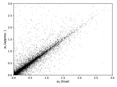
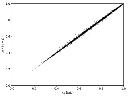
Figure 1: Left-side plot: correlation between true and approximated $\alpha_{1}$ calculated for the $a_{1}^{\pm}-\rho^{\mp}$. right-side plot: Correlation between fraction $x$ of $\tau$ lepton momentum carried by hadronic decay products obtained in the Approx-1 approximation; in the $a_{1}^{\pm}-\rho^{\mp}$ and laboratory frames.

3.2 Energy and transverse component of neutrino momenta

Now, with the help of approximated $p_{\nu}^{z}$ (the component longitudinal along visible decay products), we can turn our attention to $p_{\nu}^{x}$ and $p_{\nu}^{y}$. In the hadronic decay products system rest-frame the $p_{{had}_{1,2}}$ momenta are set along the $z$ direction thus $p_{had}^{x}=p_{had}^{y}=0$. The $\tau$ mass constraint reads

$$m_{\tau}^{2}=(E_{\nu}+E_{had})^{2}-(p_{\nu}^{x})^{2}-(p_{\nu}^{y})^{2}-(p_{\nu}^{z}+p_{had}^{z})^{2},$$ (15)

and for massless $\nu_{\tau}$

$$0=(E_{\nu})^{2}-|p^{T}_{\nu}|^{2}-(p^{z}_{\nu})^{2}.$$ (16)

The equations lead to the following relations:

$$E_{\nu} =\ \ \frac{m_{\tau}^{2}-E_{had}^{2}+(p_{had}^{z})^{2}+2\cdot p_{\nu}^{z}p_{had}^{z}}{2E_{had}},$$ (17)

$$p^{T}_{\nu} =\ \ \sqrt{E_{\nu}^{2}-(p_{\nu}^{z})^{2}},$$

where for $p_{\nu}^{z}=\alpha\cdot p_{had}^{z}$ one of the $\alpha$ approximations from Section 3.1.3 is used.

The $\alpha_{1},\alpha_{2}$, $E_{\nu_{1}}$ and $E_{\nu_{2}}$ must be positive, otherwise the approximation fails and the event can not be used. Also events with negative approximated $(p^{T}_{\nu})^{2}$ could be rejected, but for our studies we decided to set this component to zero instead. In total, about $17\%$ events are rejected for Approx-1. An additional $11\%$ are rejected when for each event it is requested that with Approx-2 and Approx-3 the above criteria are also fulfilled. In Fig. 2, the distribution of relative shifts from generated to approximated $E_{\nu},p^{z}_{\nu},p^{T}_{\nu}$ is given for the $a_{1}^{\pm}-\rho^{\mp}$ case. The $p^{T}_{\nu}$ is approximated better than $E_{\nu},p^{z}_{\nu}$. We remain encouraged because for ML classifications even approximate observables (expert variables) may be useful to improve classification scores.

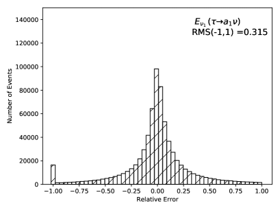
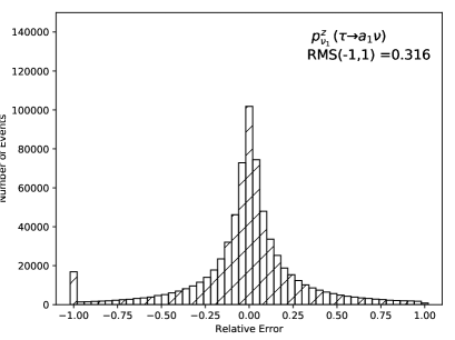
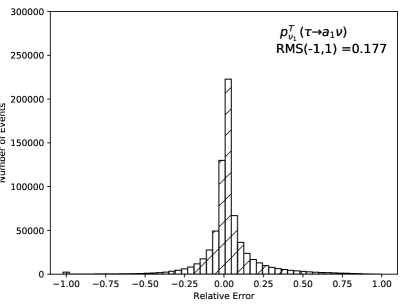
Figure 2: The $(x_{true}-x_{approx.})/x_{true}$ distribution for the reconstructed neutrino energy (left), longitudinal (right) and transverse (bottom) momenta; Approx-1 was used. Events of shifts outside (-1.0, 1.0) window are cumulated at -1.0 bin. The standard deviation denoted as (RMS) is calculated for the (-1.0, 1.0) range.

3.3 Azimuthal angles of neutrinos

At this point, we are left without two azimuthal angles for the orientation of $p^{T}_{\nu_{1}}$ and $p^{T}_{\nu_{2}}$ only. To capture the sensitivity of the Higgs boson CP they have to be known, preferably in the visible $\tau$-pair decay products rest-frame. Those two angles can be inferred from the $\tau$ decay vertices positions and then through boosts and rotations related to the azimuthal angles in visible decay products frame.

The transverse coordinates of the primary interaction point are to a good precision consistent with zero. At the same time, the tracks of the $\tau$ decay products will not point to this interaction vertex but to the position of the $\tau$ decay vertex shifted by the $\tau$ flight. The direction of the $\tau$ flight can be reconstructed, and as a consequence, so can be its momentum components. This provides a constraint on the $\nu_{\tau}$ momentum as well. We do not intend to go into details of this challenging secondary vertex position measurement. Let us point to Ref. [29, 30], which discuss a similar problem of secondary vertex in case of B-meson decay and its application for the classification of hadronic jets. One may assume that such measurement is possible for a $\tau$ lepton, and that the orientation of $\nu_{\tau}$ momentum around the direction of visible hadronic $\tau$ decay products can be constrained.

To access how precisely we need to know this information we take the true azimuthal angles $\phi_{\nu_{1}}$, $\phi_{\nu_{2}}$ in the rest-frame of visible decay products and smear them. For  $\Delta\phi_{\nu}=|\phi_{\nu}^{smear}-\phi_{\nu}^{true}|$ smearing probability we take

$$f_{train}(\Delta\phi_{\nu},\beta)=\frac{1}{\beta}\ exp(-\frac{1}{\beta}\Delta\phi_{\nu}).$$ (18)

We have chosen the exponential shape, instead of often used Gaussian shape . Note however that the length of the $\tau$ flight path follows an exponential distribution. We choose the sign for the shift with equal probabilities.

We think, that at present it is premature to attempt realistic detector smearing. Only in case of $\tau^{\pm}\to\pi^{\pm}\pi^{\pm}\pi^{\mp}\nu$ decay channel of the $Z/\gamma^{*}\to\tau\tau$ production, at LHC such attempts on investigating experimental smearings for secondary vertex position are reported [41].

3.4 Ansatz for direction of the $\tau$ leptons

In Subsection 3.3 above we have discussed the possibility of adding approximate information on the angle of the outgoing neutrino in the decay plane to the features list. However, for the multi-variate methods, this angle does not have to be present explicitly in the feature list. In fact, indirect information such as approximated direction of the outgoing $\tau$ lepton may be good enough.

From the primary and secondary vertex positions, direction of the laboratory system $\tau$ lepton momentum, i.e. $p_{x},p_{y},p_{z}$, is constrained. Assuming known $\tau$ time of flight ($t_{flight}$) and mass $m_{\tau}$, we calculate

$$p_{i}^{\tau}=m_{\tau}\cdot(i_{sec.\ vtx}-i_{prim.\ vtx})/t_{flight},$$ (19)

where $i_{sec.\ vtx},i_{prim.\ vtx}$ denote spatial position of the reconstructed primary and secondary vertex respectively in the laboratory (collision) frame ($i=x,y,z$). Instead of unknown true time-of-flight, we use the one of PDG [42]: $c\tau_{\tau}=87\mu m$. The true time-of-flight behaves according to the exponential distribution with mean $<t_{flight}>$ = $\tau_{\tau}$. It imposes that the approximation used for estimating $p_{x},p_{y},p_{z}$ is also characterised by an exponential distribution, with mean and sigma close to their true values. The energy of the $\tau$ lepton is then calculated using $\tau$ mass constraint

$$E^{\tau}=\sqrt{(p_{x}^{\tau})^{2}+(p_{y}^{\tau})^{2}+(p_{z}^{\tau})^{2}+m_{\tau}^{2}}.$$ (20)

Now, the complete 4-momentum of each $\tau$ is boosted into the $\rho^{\pm}-\rho^{\mp}$, $a_{1}^{\pm}-\rho^{\mp}$ or $a_{1}^{\pm}-a_{1}^{\mp}$ system rest-frame and added to the feature lists for DNN training.

4 Classification with DNN

The structure of the data and neural network architecture follows [20]. We start from the code used there. For the convenience of the reader, we summarise the technical description of our DNN model in Appendix A.

Simulated data consist of events where all decay products are stored together with their flavours. The four-momenta of the laboratory frame are stored and, whenever it is needed, transformed to respective rest-frames as explained in Section 2. With respect to the analysis published in [20] we explore approximate information on neutrino momenta derived from the kinematical constraints of the Higgs decay products. We show that significant improvement may originate from even very inaccurate information on the azimuthal angles of the neutrinos’ directions.

We explore the potential of classification with the DNN technique with several variants of the feature lists as detailed in Table 2. They are grouped and marked as Variant-X.Y, where X labels a choice of the main features and Y in most cases labels if they are calculated from the generator-level 4-momenta or from the approximation; it may also mark if additional, high-level, variables were used. It gives us very useful handles to quantify how much of the DNN performance we are loosing due to certain approximations made on the groups of features.

Table 2: Lists of features for ML classification, marked as Variant-X.Y. In the third column, number of features respectively for the $\rho^{\pm}-\rho^{\mp}$, $a_{1}^{\pm}-\rho^{\mp}$ and $a_{1}^{\pm}-a_{1}^{\mp}$ channels are given. All components of the 4-momenta are taken in the hadronic decay products rest-frame. Primary resonances ($\rho^{\pm}$, $a_{1}^{\pm}$) aligned with the $z$ axis. The $E^{x}_{miss}$, $E^{y}_{miss}$ are of the laboratory frame. In practice, instead of $p_{\nu}^{T}$ and $\phi_{\nu}$, the pair of variables $p_{\nu}^{T}\cos\phi_{\nu}$, $p_{\nu}^{T}\sin\phi_{\nu}$ is used.

Notation	Features	Counts	Comments
Variant-All	4-momenta ($\pi^{\pm},\pi^{0},\nu$)	24/28/32
Variant-1.0	4-momenta ($\pi^{\pm},\pi^{0}$)	16/20/24	as in Table 3 of [20]
Variant-1.1	4-momenta ($\pi^{\pm},\pi^{0},\rho^{\pm},a_{1}^{\pm}$), $m_{i}^{2},m_{k}^{2},y_{i},y_{k},\phi^{*}_{i,k}$	29/46/94
Variant-2.0	4-momenta ($\pi^{\pm},\pi^{0}$), $E_{\nu}$, $p^{z}_{\nu}$,$p^{T}_{\nu}$	22/26/30
Variant-2.1	4-momenta ($\pi^{\pm},\pi^{0}$), $E_{\nu}$, $p^{z}_{\nu}$,$p^{T}_{\nu}$	22/26/30	Approx. $E_{\nu},p_{\nu}^{z},p_{\nu}^{T}$
Variant-2.2	4-momenta ($\pi^{\pm},\pi^{0}$), $E_{\nu}$, $p^{z}_{\nu}$,$p^{T}_{\nu}$, $E^{x}_{miss}$, $E^{y}_{miss}$	24/28/32	Approx. $E_{\nu}^{z},p_{\nu},p_{\nu}^{T}$
Variant-3.0.0	4-momenta ($\pi^{\pm},\pi^{0}$), $E_{\nu}$, $p^{z}_{\nu}$, $p^{T}_{\nu}$, $\phi_{\nu}$	24/28/32	Approx. $E_{\nu},\vec{p_{\nu}}$
Variant-3.1.$\beta$	4-momenta ($\pi^{\pm},\pi^{0}$), $E_{\nu}$, $p^{z}_{\nu}$, $p^{T}_{\nu}$, $\phi_{\nu}$	24/28/32	Approx. $E_{\nu},\vec{p_{\nu}}$; $\phi_{\nu}$ smeared with $\beta$
Variant-4.0	4-momenta ($\pi^{\pm},\pi^{0}$, $\tau^{\pm}$)	24/28/32
Variant-4.1	4-momenta ($\pi^{\pm},\pi^{0}$, $\tau^{\pm}$)	24/28/32	Approx. $p_{\tau}$

In Table 3, we collect AUC scores and Average Precision Scores (APS) [39], obtained on the test sample of simulated data (i.e. events not used for training or validation) with the DNN trained on 50 epochs and with dropout = 0.20. Both are comparable, the APS score being systematically slightly lower, except for few cases of the $a^{\pm}_{1}-a^{\mp}_{1}$ channel. This configuration was found as most stable for comparison of Variant-X.Y classifications, but not necessarily represents the optimal performance of the particular variant of the features list. In the first line of Table 3 we recall the oracle predictions , for details see Appendix A. It cannot be outperformed by the DNN of any Variant-X.Y. It may not be reached even with a features list containing the complete set of 4-momenta of $\tau$ decay products, denoted as Variant-All.

In the following subsections we discuss those results in detail.

Table 3: The AUC and APS scores to discriminate scalar from pseudo-scalar CP state of the Higgs boson, obtained on the test sample. The DNN was trained on 50 epochs and dropout=0.2 (except explicitly marked case of Variant-All). Results for $\rho^{\pm}-\rho^{\mp}$, $a_{1}^{\pm}-\rho^{\mp}$ and $a_{1}^{\pm}-a_{1}^{\mp}$ channels are given. The first column labels choice of features. For details see Table 2.

Features	AUC/APS	AUC/APS	AUC/APS
list	($\rho^{\pm}-\rho^{\mp}$)	($a_{1}^{\pm}-\rho^{\mp}$)	($a_{1}^{\pm}-a_{1}^{\mp}$)
Oracle predictions	0.784/0.785	0.781/0.783	0.780/0.782
Variant-All (drop=0.0)	0.784/0.786	0.778/0.778	0.773/0.774
Variant-All	0.769/0.764	0.748/0.742	0.728/0.720
Variant-1.0	0.655/0.654	0.603/0.602	0.573/0.578
Variant-1.1	0.656/0.655	0.609/0.607	0.580/0.585
Variant-2.0	0.663/0.663	0.626/0.625	0.594/0.595
Variant-2.1	0.664/0.666	0.622/0.622	0.591/0.593
Variant-2.2	0.664/0.666	0.622/0.622	0.591/0.593
Variant-3.0.0	0.771/0.771	0.749/0.743	0.728/0.721
Variant-3.1.2	0.760/0.759	0.738/0.730	0.718/0.710
Variant-3.1.4	0.738/0.735	0.714/0.705	0.687/0.677
Variant-3.1.6	0.715/0.713	0.689/0.680	0.660/0.652
Variant-4.0	0.769/0.766	0.748/0.742	0.728/0.720
Variant-4.1	0.738/0.733	0.704/0.696	0.683/0.676

4.1 Benchmarks using all or only hadronic decay products

For the first benchmark each event is represented with 4-momenta of both $\tau$-leptons decay products (including neutrinos) in the rest-frame of all hadronic decay products combined. This set of features is denoted as Variant-All. Results are displayed in the second and third line of Table 3. The DNN should be able to reproduce oracle predictions, which is almost the case if dropout is not used, but only approaches it with base-line configuration of dropout=0.20. The dropout is lowering DNN performance in Variant-All, but we have verified that for other feature lists it is not always the case. It helps with suppressing overfitting, as illustrated in Fig. 8 of Appendix A. In Fig. 3, left plot, we show for the $a_{1}^{\pm}-\rho^{\mp}$ channel Variant-All, the AUC score as a function of number of epochs used for training and validating. The scores up to about $0.75$ are reached for the validation sample and Variant-All.

For the second benchmark following Ref. [20], the same events but with features limited to 4-momenta of visible $\tau$ leptons decay products and quantities derived directly from them are used  . The set with only 4-momenta of visible decay products in the respective rest-frames of intermediate resonances is called Variant-1.0. If supplemented with higher-level expert features like invariant masses of intermediate resonances or energy fractions, it is called Variant-1.1. For all three channels results for Variant-1.0 and Variant-1.1 are close. Expert variables provide redundant information only. In Fig. 3 (left plot) AUC results for training and validation of $a_{1}^{\pm}-\rho^{\mp}$ are shown for Variant-1.0. The highest result on the validation sample is around $0.60$.

In Fig. 3, right plot, we show ROC curves displaying True Positive Rates (TPR) versus False Positive Rates (FPR) for Variant-All and Variant-1.0.

The achieved AUC’s and APS’s are collected in the respective lines of Table 3. The large gap of AUC and APS performance between Variant-All and Variant-1.0 feature sets, is present for all channels. In the following, we attempt to improve performance thanks to information on the neutrino momenta and in particular their azimuthal angles.

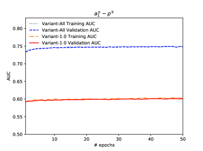
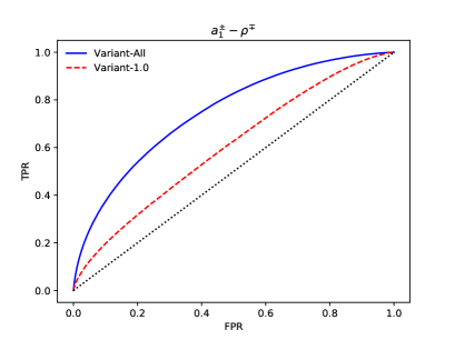
Figure 3: The AUC score (left plot) for training and validation of $a_{1}^{\pm}-\rho^{\mp}$ samples, as a function of number of epochs and ROC curve for 50 epochs (right plot). The Variant-All and Variant-1.0 were chosen for the list of features. Training and validation curves overlap.

4.2 Adding neutrino momenta

In this Subsection we present improvements due to the energy and longitudinal neutrino momenta. Such an extension of the features list is not expected to be very beneficial, as CP information is carried by the transverse degrees of freedom, but it may optimize the use of information learned from correlations of hadronic decay products.

With assumptions explained in Section 3, we approximate each of neutrino momentum components $E_{\nu}$, $p^{z}_{\nu}$, $p^{T}_{\nu}$ in the rest-frame of hadronic decay products. It is interesting to check first what is the potential impact of that information, i.e. when truth level values are used. We add the laboratory frame $E^{x}_{miss},E^{y}_{miss}$, redundant to some extend, as it was already used in Eq. (7) for $p^{z}_{\nu}$.

The augmented list of features, using true components of neutrino momenta, is denoted as Variant-2.0, while the ones using approximate components of neutrino momenta are denoted as Variant-2.1 and Variant-2.2, depending on whether the information on $E^{x}_{miss},E^{y}_{miss}$ is included or not. The AUC and APS scores by the DNN for $\rho^{\pm}-\rho^{\mp}$, $a_{1}^{\mp}-\rho^{\pm}$ and $a_{1}^{\pm}-a_{1}^{\mp}$ channels are displayed in Table 3. The improvement from Variant-1.0 to Variant-2.0 is not impressive. We observe later a small performance degradation from Variant-2.0 to Variant-2.1, which uses approximate neutrino features resulting in sensitivity loss. The laboratory frame $E^{x}_{miss},E^{y}_{miss}$ of Variant-2.2 are, as expected, of no help. In Fig. 4 we show DNN performance for the $a_{1}^{\pm}-\rho^{\mp}$ samples as a function of number of training epochs: the AUC achieved as a function of number of epochs and the ROC curves.

For the feature sets: Variant-2.1 and Variant-2.2, all three different approximations for $E_{\nu}$, $p^{z}_{\nu}$, $p^{T}_{\nu}$ were studied. The differences between Approx-1, Approx-2 and Approx-3 are small but will certainly show once detector effects are included.

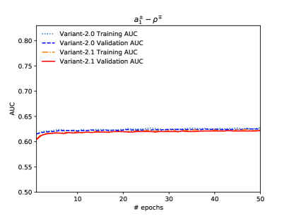
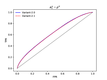
Figure 4: Left plot: the AUC score for training and validation of $a_{1}^{\pm}-\rho^{\mp}$ samples, as a function of number of epochs. The Variant-2.0 and Variant-2.1 were chosen for the list of features. Right plot: the corresponding ROC curves for 50 epochs.

Clearly, the improvement from approximated information on the neutrinos energy and momenta (longitudinal and module of transverse) is rather small for all three channels. The most sensitive information on the CP state lies in azimuthal angles of the individual neutrinos. That is in individual $p^{x}_{\nu},p^{y}_{\nu}$ components of hadronic decay products rest-frame and not in $p^{T}_{\nu}=\sqrt{(p^{x}_{\nu})^{2}+(p^{y}_{\nu})^{2}}$. Realistically any information on the individual $p^{x}_{\nu},p^{y}_{\nu}$ could be reconstructed only if the measurement of the $\tau$ decay vertices was possible. In the next Section, we evaluate how accurately this information has to be known to become useful. It constitutes a separate experimental challenge. Note that at this step, all components of $\nu_{\tau}$ momenta except individual $p^{x}_{\nu},p^{y}_{\nu}$ are reconstructed sufficiently well from the measurable quantities.

4.3 Azimuthal angles of neutrinos from decay vertices

The azimuthal angles $\phi_{\nu_{1}}$, $\phi_{\nu_{2}}$ can be obtained from the measurement of the $\tau$ lepton decay vertices. It allows to reconstruct the $\tau$-lepton momenta and hopefully can be used for our purpose as well. This is rather widely used technique in the experimental measurements, see e.g. [43], but so far for $\tau$-mass or $\tau$-lifetime measurement rather than for neutrino azimuthal angles.

We do not aim to reconstruct those angles, we simply calculate them from the neutrinos 4-momenta and add to the feature lists  Variant-3.0 and Variant-3.1.$\beta$. The first one is when the true $\phi_{\nu_{1}}^{true}$, $\phi_{\nu_{2}}^{true}$ are used, and the second one is with smeared $\phi_{\nu_{1}}^{smear}$, $\phi_{\nu_{2}}^{smear}$. In Fig. 5 the $\phi_{\nu}^{true}-\phi_{\nu}^{smear}$ distribution for $\beta=0.4$ of Eq. (18) is shown.

The AUC scores are evaluated for the $\beta$ in $(0,2)$ range. In Fig. 6 the AUC’s for test samples of the three channels are given as a function of $\beta$. The AUC scores for $\beta=0.0$ reproduce, as they should, the ones of Variant-3.0 and are not very far from scores of Variant-All. That is because the only difference is approximate information on energy, longitudinal and transverse momenta of the neutrino. For $\beta$ above 1.4, the AUC decrease to the ones of Variant-2.1 sets, which is then equivalent to not having information on the neutrino azimuthal angles at all. Even $\phi_{\nu_{1}}^{smear}$, $\phi_{\nu_{2}}^{smear}$, corresponding to rather large $\beta=0.$4 contributes sizably to CP Higgs sensitivity.

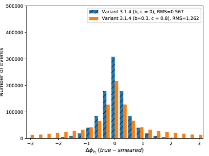
Figure 5: The (true - smeared) distribution of $\Delta\phi_{\nu_{1}}$ for $\beta$=0.4 with/without additional polynomial modulation of Eqs. (4.3)/(18).

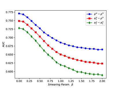
Figure 6: The AUC in function of smearing parameter $\beta$ of Eq. (4.3) for $\rho^{\pm}-\rho^{\mp}$, $a_{1}^{\pm}-\rho^{\mp}$ and $a_{1}^{\pm}-a_{1}^{\mp}$ channels and $Variant-3.1.\beta$.

The derivative of the sensitivity with respect to $\beta$, reaches its maximum at about $0.35$ and remains constant until $\beta=0.9$. Then nearly all sensitivity gain is lost. For even larger $\beta$, loss of sensitivity continues, but as the contribution is then already small, deterioration is small too.

Let us now check if the DNN algorithm is sensitive to precise modeling of the $\phi_{\nu_{1,2}}$ resolution. That is why, for the validation and test sample, we introduce  an additional polynomial component for the smearing

$$f_{valid}(\Delta\phi_{\nu},\beta,b,c)=f_{train}(\Delta\phi_{\nu},\beta)\bigl{(}1+b^{2}\Delta\phi_{\nu}^{2}+c^{2}\Delta\phi_{\nu}^{4}\bigr{)}.$$

The results should mimic the impact of inefficiencies (mismodeling) of the DNN training sample with respect to what is present in the validation or test samples. In Fig. 5 the distribution of $\phi_{\nu}^{true}-\phi_{\nu}^{smear}$ is given for $\beta=0.4,$ and $b,c=0.3,\;0.8$. In Table 4 results for $\rho^{\pm}-\rho^{\mp}$, $a_{1}^{\pm}-\rho^{\mp}$, $a_{1}^{\pm}-a_{1}^{\mp}$ channels and for $\beta$ = 0.2, 0.4, 0.6 with further choices of $b$ and $c$ are collected. The additional polynomial component of smearing introduced to the test sample is not affecting the DNN performance. We can see that the degradation due to $b,c=0.3,\;0.8$ is small and the results provide some encouraging insight to the DNN capacity to exploit imprecise information and point to possible direction for the studies of systematic uncertainities .

In our study, when precision of experimental inputs was expected to be better than that from decay vertices impact parameters, we have reconstructed neutrino momenta components from hadronic products and conservation laws. Only the $\phi_{\nu}$ angles required this rather low precision input. From Fig. 6 we can expect that approximate $\phi_{\nu}$ angle with ambiguity of up to $\pm\frac{\pi}{4}$ may sizably improve sensitivity.

Such conjecture on the size of $\phi_{\nu}$ smearing critical for CP sensitivity is of interest for any ML application. For $\beta=1.2$ the shift $\Delta\phi_{\nu}$ was bigger than $\frac{\pi}{4}$ in sizable fraction of events. Then; DNN solution does not gain sensitivity from $\phi_{\nu}$. Still, an approach relying less on $\phi_{\nu}$ measurement, but on restricting, which events should be dropped from the analysis could be useful. Possibly, for large smearing, elimination of events with high risk of $\phi_{\nu}$ misreconstruction may be appropriate as it was attempted in Ref. [14]. A discussion of physics properties simultaneously with those of the ML algorithms may be of interest again.

Table 4: The AUC and APS for $\rho^{\pm}-\rho^{\mp}$, $a_{1}^{\pm}-\rho^{\mp}$ and $a_{1}^{\pm}-a_{1}^{\mp}$ channels with features Variant - 3.1.$\beta$ ($\beta$ = 0.2, 0.4 and 0.6 is used for training, validation and test samples). For the test sample polynomial modifications of smearing function, Eq. (4.3), were introduced.

	AUC / APS
Parameters	($\beta=0.2$)	($\beta=0.4$)	($\beta=0.6$)
	$\rho^{\pm}-\rho^{\mp}$
b = 0.0, c = 0.0	0.761/0.759	0.739/737	0.715/0.714
b = 0.3, c = 0.8	0.760/0.758	0.739/0.736	0.716/0.713
b = 0.9, c = 0.9	0.759/0.756	0.738/0.734	0.714/0.713
	$a_{1}^{\pm}-\rho^{\mp}$
b = 0.0, c = 0.0	0.739/0.731	0.714/0.706	0.687/0.679
b = 0.3, c = 0.8	0.738/0.730	0.714/0.705	0.687/0.679
b = 0.9, c = 0.9	0.737/0.728	0.714/0.704	0.687/0.678
	$a_{1}^{\pm}-a_{1}^{\mp}$
b = 0.0, c = 0.0	0.713/0.705	0.690/680	0.660/0.653
b = 0.3, c = 0.8	0.715/0.706	0.693/0.682	0.661/0.653
b = 0.9, c = 0.9	0.714/0.706	0.688/0.680	0.660/0.653

4.4 Tau lepton direction

The approximate information on the $\tau$ lepton direction enables the DNN to constrain the neutrino and significantly improve the classification. For that Variant-4.0 and Variant-4.1 are defined in Table 2.

In Table 3, performances of the DNN are presented, when true level, or from approximation, $\tau$ lepton spatial momenta components in the respective $\rho^{\pm}-\rho^{\mp}$, $a_{1}^{\pm}-\rho^{\mp}$ and $a_{1}^{\pm}-a_{1}^{\mp}$ rest-frame are added. We observe significant improvement of the performance with respect to Variant-2.1 and comparable to Variant-3.1.X family. In fact, the performance of Variant-4.0 is close to Variant-All. Variant-4.1 is a bit lower, close to Variant-3.1.4. Then only $\tau$ direction in the laboratory frame is exact and the energy is obtained from the simple ansatz of Subsection 3.4. When such $\tau$ 4-momentum is boosted to $\rho^{\pm}-\rho^{\mp}$, $a_{1}^{\pm}-\rho^{\mp}$ and $a_{1}^{\pm}-a_{1}^{\mp}$ rest-frame, its direction absorbs some biases. Results of Variant-4.1 indicate that DNN efficiently converts such an input into information on $\nu_{\tau}$.

5 Summary

From the perspective of theoretical modeling, the CP parity phenomenology in cascade $H\to\tau\tau$, $\tau^{\pm}\to had^{\pm}\nu_{\tau}$ decay is rather simple, because the matrix element can be easily defined. On the other hand, the parity effect manifests itself in rather complicated features of multi-dimensional distributions where kinematic constraints related to ultra-relativistic boosts and detection ambiguities play an important role in the reconstruction of the $\tau$ decay kinematic. Our aim was to evaluate what level of precision and for each experimentally available features need to be achieved by experiments for the meaningful measurements.

In our previous paper [20] we have studied the performance of the DNN binary classification technique for the hadronic $\tau$ leptons decay products only. Now we have turned our attention also to the $\nu_{\tau}$ momenta.

Whenever possible, we have exploited constraints of $\tau$-mass, $H$-mass and energy momentum conservation to minimize dependence on highly smeared neutrino kinematic deduced from the impact parameter of $\tau$ decay and production vertices. The resulting set of expert variables helps DNN algorithms to identify physics sensitive variables useful to identify differences between the event classes.

Reconstructed with approximation but from visible decay products, longitudinal components of the neutrino momenta alone improved the AUC from 0.656, 0.609, 0.580 to about 0.664, 0.622, 0.591 respectively for $\rho^{\pm}-\rho^{\pm}$, $a_{1}^{\pm}-\rho^{\mp}$ and $a_{1}^{\pm}-a_{1}^{\mp}$ cases. The improvement for the Higgs boson CP sensitivity is rather minuscule, even when the detector effects were not taken into account.

A more significant improvement came when the transverse components of the neutrino momenta were known, even imprecisely. This can be achieved if the $\tau$-lepton decay vertices are measured and used to reconstruct directions of the $\tau$ leptons momenta. The performance of such reconstruction is detector specific and is a challenge. We have estimated how big of an improvement of CP sensitivity is obtained as a function of detection smearing for the azimuthal angles $\phi_{\nu}$ and $\phi_{\bar{\nu}}$. Even with large smearing, $\beta=0.4$, the AUC improved from 0.664, 0.622 and 0.591 to about 0.738, 0.714 and 0.687 for $\rho^{\pm}-\rho^{\pm}$, $a_{1}^{\pm}-\rho^{\mp}$ and $a_{1}^{\pm}-a_{1}^{\mp}$ cases, respectively. Note that $\phi_{\nu}$ and $\phi_{\bar{\nu}}$ angles represent an intermediate step in the quest: from expert variables to DNN algorithms with direct use of low-level features. We are leaving the topic of the angles measurements and use for forthcoming works.

Similar performance is expected when good quality $\tau$ lepton laboratory frame direction, as seen in the rest-frame of all visible Higgs decay products combined is available for the evaluation of $\tau$ direction. The ambiguity on the laboratory frame $\tau$ energy is not that important. The enhancement with $\tau^{\pm}$ directions was achieved (Variant-4.1), the AUC reached 0.738, 0.704 and 0.683 respectively for $\rho^{\pm}-\rho^{\pm}$, $a_{1}^{\pm}-\rho^{\mp}$ and $a_{1}^{\pm}-a_{1}^{\mp}$ cases.

In Fig. 7 we show ROC curves for different variants of feauture lists discussed in this paper.

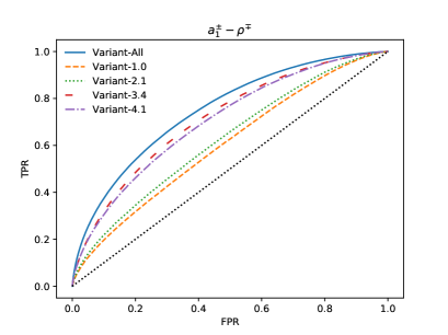
Figure 7: The ROC curves for different feauture lists.

The concept of the optimal observables is used since many years to obtain phenomenologically sound results. For ML classification, where multi-dimensional input is used, it provides essential tests. An approach, where sophisticated methods are used to measure $h_{\pm}$ of Eq. (2), should be mentioned. All complexity of hadronic $\tau$ decays and detector response is then hidden in each $\tau^{\pm}$ polarimetric vector $h_{\pm}$. Once an algorithm for $h_{\pm}$ reconstruction prepared, the later step of CP phenomenology is straightforward: details of $\tau^{\pm}$ decay channels and detector effects are resolved. The $h_{\pm}$ complexity is smaller than of the whole $H\to\tau\tau$ cascade decay. It is independent from the Higgs phenomenology and preparation can rely on the much more abundant $Z\to\tau\tau$ data. Such a possibility was mentioned in [44] and is pursued e.g. by the CMS collaboration. Then, the ML learning techniques could be used to reconstruct $h_{\pm}$ vectors from the complex detector responses to particular $\tau$ decay channels and details of its decay vertex position.

The evaluation which of the methods is best, or in fact, how complementary the methods can be, requires work of experimental groups.

Recently, in Ref. [45], classifiers specifically tuned to tackle the Lorentz group features of High Energy Physics signatures were prepared and used. This could be useful for Variant-1.0, where four momenta of secondary $H\to\tau\tau$ decay products are used only. In the present work this may be less straightforward as part of the features is intimately related to laboratory frame and their transformation to other frames may be poorly defined. That is why, expert variable style reconstruction of neutrinos azimuthal angles may be an efficient way to follow, or at least useful to better understand limitations and ambiguities of methods.

Acknowledgments

P. Winkowska would like to thank L. Grzanka for valuable comments and suggestions through the time of preparing results.

This project was supported in part from funds of Polish National Science Centre under decisions DEC-2017/27/B/ST2/01391. DT and PW were supported from funds of Polish National Science Centre under decisions DEC-2014/15/B/ST2/00049.

Majority of the numerical calculations were performed at the PLGrid Infrastructure of the Academic Computer Centre CYFRONET AGH in Krakow, Poland.

Appendix A Deep Neural Network

The structure of the simulated data and the DNN architecture follows what was published in our previous paper [20]. It is prepared for TensorFlow [46], an open-source machine learning library. The learning procedure is optimized using a variant of the stochastic gradient descent algorithm called Adam [47]. We also use Batch Normalization [48] (which has regularization properties) and Dropout [49] (which prevents overfitting) to improve the training of the DNN. The problem of determining Higgs boson CP state is framed as binary classification because the aim is to distinguish between the two possible scalar and pseudoscalar Higgs CP states.

We consider three separate problems for $H\to\tau\tau$ channels: $\rho^{\pm}-\rho^{\mp}$, $a_{1}^{\pm}-\rho^{\mp}$, $a_{1}^{\pm}-a_{1}^{\mp}$. We solve all three problems using the same neural network architecture. Depending on the decay channel for the outgoing $\tau$ pairs, each of the cases contains different number of dimensions to describe an event, i.e. production of the Higgs boson decaying into $\tau$ lepton pair. Each data point consists of features which represent the observables/variables of the consecutive event. The data point is thus an event of the Higgs boson production and decay into $\tau$ lepton pair. The structure of the event is represented as follows:

$$x_{i}=(f_{i,1},...,f_{i,D}),w_{a_{i}},w_{b_{i}}$$ (21)

The $f_{i,1},...,f_{i,D}$ represent numerical features and $w_{a_{i}},w_{b_{i}}$ are weights proportional to the likelihoods that an event comes from a set $A$ or $B$ (binary scalar or pseudoscalar classification). The weights calculated from the quantum field theory matrix elements are available and stored in the simulated data files. This is a convenient situation, which does not happen in many other cases of ML classification. The $A$ and $B$ distributions highly overlap in the $(f_{i,1},...,f_{i,D})$ space, a more detailed discussion can be found in [20]. The perfect separation is therefore not possible and $w_{a_{i}}/(w_{a_{i}}+w_{b_{i}})$ corresponds to the Bayes optimal probability that an event is sampled from set $A$ and not $B$. The $w_{a_{i}},w_{b_{i}}$ are used to compute targets during the training procedure.

Because model A and B samples are prepared with the same events and differ with the spin weights $w_{a_{i}},w_{b_{i}}$ only, the statistical fluctuations of the learning procedure are largely reduced. It has also consequences for the actual implementation of the DNN metric and code.

To quantify classification performance, weighted AUC and APS were used , we have not followed further alternatives. For each data point $x_{i}$, the DNN returns probability $p_{i}$ that it is correctly (not correctly) classified as of type A and it contributes to the final loss function twice, with weight $w_{a_{i}}$ and $w_{b_{i}}$ respectively. With this definition, the AUC = 0.5 would be obtained for random assignment, while the AUC = 1.0 would be reached for perfect separation. As in the studied problems distributions are overlapping, the best achievable AUC$\simeq 0.78$ is reached only with $p_{i}=w_{a_{i}}/(w_{a_{i}}+w_{b_{i}})$ (oracle predictions). The value depends slightly on the case studied, due to applied minimal set of cuts on the kinematics of $\tau$ decay products to partly emulate detector conditions.

Weighted events with $w_{a},w_{b}$ are used for implementation convenience and to limit statistical fluctuations. We have repeated some of the DNN classification chain (training, validation, testing) using unweighted events  too. We have found very good consistency of performance achieved in this way.

The DNN architecture , consists of D-dimensional input (list of features) followed by six layers of 300 nodes each with ReLU [50] activation functions and 1-dimensional output layer returning probability $p_{i}$ of the choice. It is calculated using the softmax function. The metric minimized by the model is negative log likelihood of the true targets under Bernoulli distributions.

The parameter which was optimized with respect to what was used in [20] was a dropout [49]. For the analysis presented in Ref. [20] AUC score was obtained after training with 5 epochs. It was considered sufficient. Here, given the variety of feature lists, we performed training on much larger number of epochs and studied what would be the optimal working point for number of epochs and dropout. The 20% dropout seemed to be the optimal choice to avoid overfitting, which occurs in the case of a larger number of training epochs. The best performance was achieved after 5-50 epochs, depending on the case. Training with 50 epochs was used on the test samples to quote the final AUC score. While optimizing dropout level, we have observed that although it leads to more robust DNN (smaller risk for overfitting), the performance was sometimes somewhat reduced. The positive impact of dropout is illustrated (on dataset consiting of 1M event samples) in Fig. 8 for $\rho^{\pm}-\rho^{\mp}$ channel and Variant-1.1 of training and validation.

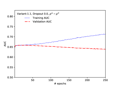
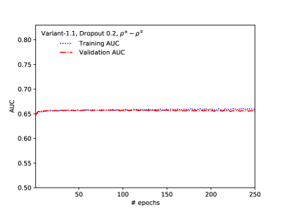
Figure 8: The DNN training and validation AUC as a function of number of epochs, for $\rho^{\pm}-\rho^{\pm}$ channel and sample features Variant-1.1, without dropout (left plot) and with dropout $=0.2$ (right plot).

Appendix B Alternative ML techniques

Although Deep Neural Networks are often used for classification tasks in High Energy Physics, many other more classical techniques are used as well and often are able to achieve similar classification performance. Despite promising results that are often enlisted in papers, one should always remember that a Machine Learning technique that perform well on one data-set with specific features, may deliver not so promising results on the other.

This observation is of fundamental nature and results from the mathematical assumption behind particular ML libraries. The solutions which were developed for the libraries, depend on the application domains the particular systems were prepared for. Ref. [51] can be used as a guidance. The recent study [52] collected extensive comparison of several Machine Learning algorithms. Despite not being able to contribute much to that topic, we show that for the application discussed through this paper it is indeed the case: the DNN technique by far outperforms the more classical approaches.

The following Machine Learning techniques were chosen for the comparative study:

• Boosted Trees (BT) [34]

• Random Forest (RF) [35]

• Support Vector Machine (SVM) [36]

For Boosted Trees the XGBoost [34] library was used while for SVM and Random Forest the scikit-learn [53] was chosen.

The AUC score was used to evaluate performance of ML methods. This is one of the recommended approaches when using a single number in evaluation of Machine Learning algorithms on binary classification problems. To minimize bias the comparisons were carried out on the same data-sets .

For the Boosted Trees method the point of interest was to check the dependence of obtained results on the depth of a tree. The AUC score as a function of a tree depth is given on Fig. 9 for the $\rho^{\pm}-\rho^{\mp}$ case and several variants of the feature list. As bigger depth affects complexity of computation, a search for optimal choice both in terms of results and efficiency of computation was performed. Tree depth between 3 and 10 is suggested in [34]. At first we have used depths from 3 to 20. The upper bound was increased to see the trend on AUC score plots. The results seemed to rise up to 20. Additional evaluation with the depth equal to number of features of a given Variant-X.Y was also carried out.

As suggested in the literature [54], for the Random Forest method 128 trees (estimators) were used. For the next best split during the tree building number of features equal to $log_{2}(N_{f})$ or $\sqrt{N_{f}}$, where $N_{f}$ denotes number of features, was tried. Performances of the two choices were comparable. For the trees depth the optimal value, as found for Boosted Trees was used. Tests with a larger number of trees (300) and bigger tree depths (30) were also carried out.

For the Support Vector Machine method, first tests were performed to determine which kernel, linear or RBF, gives more promising results. This resulted in choice of RBF kernel with better results stability. In the next step fine-tuning of $C$ and $\gamma$ parameters (soft margin and kernel parameter) was performed. The parameters evenly distributed on logarithmic scale from $10^{-3}$ to $10^{3}$ were tested. To avoid excessive computation, fine-tuning was performed only for Variant-All, and on smaller event sample. The obtained parameters, $C$ = 10 and $\gamma$ = 0.1, were then used to train the classifier on other feature lists as well.

The comparison of best performance for the $\rho^{\pm}-\rho^{\mp}$ channel and different variants of features is shown in Table 5. Clearly performance of the DNN is outstanding.

Table 5: AUC score for different ML methods and different feature sets obtained on validation $\rho^{\pm}-\rho^{\mp}$ sample.

Features set	DNN	BT	RF	SVM
Variant-All	0.764	0.641	0.626	0.635
Variant-1.0	0.655	0.569	0.567	0.559
Variant-2.1	0.657	0.564	0.564	0.572
Variant-2.2	0.657	0.562	0.559	0.568

We have compared execution times, memory usage and efficiency of all the classifiers. We have used the Prometheus cluster [55]. Jobs were executed at 1 node with 4 tasks per node and 5GB memory per task. The comparison is reported in Table 6. The SVM training took by far the longest time. Training of BT took the least time, under 10 minutes, which made it 8 times faster to train than DNN. Both DNN and RF used the resources well, achieving efficiency of 68.8% and 96.1% respectively.

Training time largely vary between the ML methods. This is probably due to unexpected by ML relations between features. The Higgs CP state classification turned out to be a challenge for more classical ML algorithms.

Table 6: Time of training, memory usage and efficiency information as reported by job submission system. The $\rho^{\pm}-\rho^{\mp}$ sample with the Variant-1.0 features was used and different ML methods were compared. The set of 800k training data points was used for DNN, BT and RF, while for SVM only 100k data-points were used.

Method	# Data	Training time	Memory usage	Efficiency
	points	(h:min:sec)	(% of 20GB)	(CPU)
DNN	800 k	01:21:58	6.3%	68.8%
SVM	100 k	01:52:03	4.3%	25.0%
BDT	800 k	00:09:40	9.6%	24.9%
RF	800 k	00:34:25	37.9%	96.1%

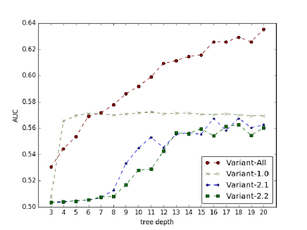
Figure 9: The AUC score of Boosted Trees classifier as a function of the tree depth.

References

- [1] D. Guest, K. Cranmer and D. Whiteson, Ann. Rev. Nucl. Part. Sci. 68, 161 (2018) doi:10.1146/annurev-nucl-101917-021019 [arXiv:1806.11484 [hep-ex]].
- [2] G. Carleo, I. Cirac, K. Cranmer, L. Daudet, M. Schuld, N. Tishby, L. Vogt-Maranto and L. Zdeborová, arXiv:1903.10563 [physics.comp-ph].
- [3] K. Albertsson et al., J. Phys. Conf. Ser. 1085 (2018) no.2, 022008 doi:10.1088/1742-6596/1085/2/022008 [arXiv:1807.02876 [physics.comp-ph]].
- [4] P. Baldi, K. Bauer, C. Eng, P. Sadowski, and D. Whiteson, Phys. Rev. D93 (2016), no. 9 094034, 1603.09349.
- [5] C. Shimmin, P. Sadowski, P. Baldi, E. Weik, D. Whiteson, E. Goul, and A. Søgaard, Phys. Rev. D96 (2017), no. 7 074034, 1703.03507.
- [6] D. Guest, J. Collado, P. Baldi, S.-C. Hsu, G. Urban, and D. Whiteson, Phys. Rev. D94 (2016), no. 11 112002.
- [7] G. Louppe, et al., 1702.00748.
- [8] K. Fraser, M. D. Schwartz, Journal of High Energy Physics10 (2018), 093. 1803.08066.
- [9] G. Kasieczka et al., SciPost Phys. 7 (2019) 014 doi:10.21468/SciPostPhys.7.1.014 [arXiv:1902.09914 [hep-ph]].
- [10] G. Kasieczka, N. Kiefer, T. Plehn and J. M. Thompson, SciPost Phys. 6 (2019) 069 doi:10.21468/SciPostPhys.6.6.069 [arXiv:1812.09223 [hep-ph]].
- [11] M. Kramer, J. H. Kuhn, M. L. Stong, and P. M. Zerwas, Z. Phys. C64 (1994) 21–30.
- [12] G. R. Bower, T. Pierzchala, Z. Was, and M. Worek, Phys. Lett. B543 (2002) 227–234.
- [13] A. Rouge, Phys. Lett. B619 (2005) 43–49.
- [14] K. Desch, Z. Was, and M. Worek, Eur. Phys. J. C29 (2003) 491–496, hep-ph/0302046.
- [15] S. Berge and W. Bernreuther, Phys. Lett. B671 (2009) 470–476.
- [16] S. Berge, W. Bernreuther, and S. Kirchner, Phys. Rev. D92 (2015) 096012, 1510.03850.
- [17] ATLAS Collaboration, ATL-PHYS-PUB-2019-008.
- [18] P. Baldi, P. Sadowski, and D. Whiteson, Nature Commun. 5 (2014) 4308, 1402.4735.
- [19] P. Baldi, P. Sadowski, and D. Whiteson, Phys. Rev. Lett. 114 (2015), no. 11 111801, 1410.3469.
- [20] R. Jozefowicz, E. Richter-Was, and Z. Was, Phys. Rev. D94 (2016), no. 9 093001, 1608.02609.
- [21] E. Barberio, B. Le, E. Richter-Was, Z. Was, D. Zanzi, and J. Zaremba, Phys. Rev. D96 (2017), no. 7 073002.
- [22] I. Goodfellow, Y. Bengio, and A. Courville, Deep learning. MIT Press, Cambridge, MA, 2017.
- [23] T. Przedzinski, E. Richter-Was, and Z. Was, Eur. Phys. J. C74 (2014), no. 11 3177, 1406.1647.
- [24] J. H. Kuhn, Phys. Rev. D52 (1995) 3128–3129.
- [25] ATLAS Collaboration, M. Aaboud et al., Phys. Rev. D99 (2019) 072001 1811.08856.
- [26] CMS Collaboration, S. Chatrchyan et al., JHEP 1405 (2014) 104 1401.5041.
- [27] ATLAS Collaboration, G. Aad et al., EPJC C76 (2016), 295, 1512.05955.
- [28] CMS Collaboration, A. Sirunyan et al., JINST 13 (2018) no.10, P10005. 1809.02816.
- [29] ATLAS Collaboration, G. Aad et al., JINST 11 (2016), no. 04 P04008, 1512.01094.
- [30] CMS Collaboration, A. Sirunyan et al., JINST 13 (2018) no.05, P05011. 1712.07158.
- [31] T. Sjöstrand et al., Comput.Phys.Commun. 191 (2015) 159–177 1410.3012.
- [32] N. Davidson, G. Nanava, T. Przedzinski, E. Richter-Was, and Z. Was, Comput.Phys.Commun. 183 (2012) 821–843.
- [33] P. Baldi, K. Cranmer, T. Faucett, P. Sadowski, and D. Whiteson, Eur. Phys. J. C76 (2016), no. 5 235.
- [34] T. Chen and C. Guestrin, 1603.02754.
- [35] L. Breiman, Machine Learning 45 (2001), no. 1 5–32.
- [36] A. Bevan, R. Goni, and T. Stevenson, J. Phys. Conf. Ser. 898 (2017), no. 7 072021, 1702.04686.
- [37] A. P. B. Bradley, Pattern recognition 30 (1997) 1145.
- [38] T. Fawcett, Pattern Recognition Letters 27 (2006), no. 7 861.
- [39] E. Zhang and Y. Zhang, Encyclopedia of Database Systems 2009, Springer US, page 192.
- [40] K. Desch, A. Imhof, Z. Was, and M. Worek, Phys. Lett. B579 (2004) 157–164, hep-ph/0307331.
- [41] V. Cherepanov and A. Zotz, “Kinematic reconstruction of decay in proton-proton collisions,” arXiv:1805.06988 [hep-ph].
- [42] M. Tanabashi et al. [Particle Data Group], Phys. Rev. D 98, no. 3, 030001 (2018). doi:10.1103/PhysRevD.98.030001
- [43] D. Jeans, Nucl. Instrum. Meth. A810 (2016) 51–58.
- [44] V. Cherepanov, E. Richter-Was and Z. Was, arXiv:1811.03969 [hep-ph].
- [45] M. Erdmann, E. Geiser, Y. Rath and M. Rieger, arXiv:1812.09722 [hep-ex].
- [46] M. Abadi, A. Agarwal, P. Barham, E. Brevdo, Z. Chen, C. Citro, G. S. Corrado, A. Davis, J. Dean, M. Devin, et al., Software available from tensorflow. org 1 (2015).
- [47] D. Kingma and J. Ba, arXiv:1412.6980 (2014).
- [48] S. Ioffe and C. Szegedy, arXiv:1502.03167 (2015).
- [49] N. Srivastava, G. E. Hinton, A. Krizhevsky, I. Sutskever, and R. Salakhutdinov, Journal of Machine Learning Research 15 (2014) 1929–1958.
- [50] A. F. Agarap, arXiv:1803.08375 (2018) 1803.08375.
- [51] M. Fernandez-Delgado et al., Journal of machine learning Research 15 (2014) 3133–3181.
- [52] C. Zhang, L. Changchang, Z. Xiangliang, and G. Almpanidis, Expert Systems with Applications 82 (2017) 128.
- [53] Pedregosa F. and et all, Journal of Machine learning Research 12 (2011) 2825.
- [54] T. Oshiro, P. Perez, and J. Baranauskas, “How many trees in a random forest?”, in International Workshop on Machine Learning and Data Mining in Pattern Recognition, Springer, Berlin, Heidelberg, 2012.
- [55] Prometheus computing cluster, Academic Computing Centre CYFRONET, Krakow, Poland.
- [56] M. Davier et al, Phys. Lett. B 306, 411 (1993).
- [57] P. Bialas, D. Nemeth and E. Richter-Was, arXiv:1803.00838 [cs.LG].