Remnants and ejecta of thermonuclear electron-capture supernovae

The explosion mechanism of electron-capture supernovae (ECSNe) remains equivocal: it is not completely clear whether these events are implosions in which neutron stars are formed, or incomplete thermonuclear explosions that leave behind bound ONeFe white dwarf remnants. Furthermore, the frequency of occurrence of ECSNe is not known, though it has been estimated to be of the order of a few per cent of all core-collapse supernovae. We attempt to constrain the explosion mechanism (neutron-star-forming implosion or thermonuclear explosion) and the frequency of occurrence of ECSNe using nucleosynthesis simulations of the latter scenario, population synthesis, the solar abundance distribution, pre-solar meteoritic oxide grain isotopic ratio measurements and the white dwarf mass-radius relation. Tracer particles from 3d hydrodynamic simulations were post-processed with a large nuclear reaction network in order to determine the complete compositional state of the bound ONeFe remnant and the ejecta, and population synthesis simulations were performed in order to estimate the ECSN rate with respect to the CCSN rate. The 3d deflagration simulations drastically overproduce the neutron-rich isotopes ${}^{48}\mathrm{Ca}$, ${}^{50}\mathrm{Ti}$, ${}^{54}\mathrm{Cr}$ , ${}^{60}\mathrm{Fe}$ and several of the Zn isotopes relative to their solar abundances. Using the solar abundance distribution as our constraint, we place an upper limit on the frequency of thermonuclear ECSNe as 1$-$3 % the frequency at which core-collapse supernovae (FeCCSNe) occur. This is on par with or 1 dex lower than the estimates for ECSNe from single stars. The upper limit from the yields is also in relatively good agreement with the predictions from our population synthesis simulations. The ${}^{54}\mathrm{Cr}$/${}^{52}\mathrm{Cr}$ and ${}^{50}\mathrm{Ti}$/${}^{48}\mathrm{Ti}$ isotopic ratios in the ejecta are a near-perfect match with recent measurements of extreme pre-solar meteoritc oxide grains, and ${}^{53}\mathrm{Cr}$/${}^{52}\mathrm{Cr}$ can also be matched if the ejecta condenses before mixing with the interstellar medium. The composition of the ejecta of our simulations implies that ECSNe, including accretion-induced collapse of oxygen-neon white dwarfs, could actually be partial thermonuclear explosions and not implosions that form neutron stars. There is still much work to do to improve the hydrodynamic simulations of such phenomena, but it is encouraging that our results are consistent with the predictions from stellar evolution modelling and population synthesis simulations, and can explain several key isotopic ratios in a sub-set of pre-solar oxide meteoritic grains. Theoretical mass-radius relations for the bound ONeFe WD remnants of these explosions are apparently consistent with several observational WD candidates. The composition of the remnants in our simulations can reproduce several, but not all, of the spectroscopically-determined elemental abundances from one such candidate WD.

1 Introduction

The fate of stars with initial masses between approximately 8 and 10 $M_{\sun}$ is believed to be either an oxygen-neon (ONe) white dwarf (WD) and a planetary nebula, or a neutron star (NS) and a supernova (SN) remnant (see Doherty et al., 2017, for a recent review). In the latter case, the event is called an electron-capture supernova (ECSN; Miyaji et al., 1980; Nomoto, 1987).

Electron-capture supernovae are instigated by the electron capture sequence ${}^{20}\mathrm{Ne}\rightarrow{{}^{20}\mathrm{F}}\rightarrow{{}^{20}\mathrm{O}}$ in degenerate ONe stellar cores or ONe WDs that reach the Chandrasekhar limit ($M_{\mathrm{Ch}}$). If the progenitor is an isolated star it will consist of a degenerate ONe core inside an extended H envelope, and the core will have grown to $M_{\mathrm{Ch}}$ via many recurrent thermally unstable He shell burning episodes (Ritossa et al., 1999; Jones et al., 2013). If the progenitor star was born in a close binary system its envelope can be stripped following the main sequence and the core can grow to $M_{\mathrm{Ch}}$ via stable He shell burning (Podsiadlowski et al., 2004; Tauris et al., 2015). Finally, the progenitor could also be an ONe WD stably accreting from a binary companion, retaining enough mass for the WD to reach $M_{\mathrm{Ch}}$ Schwab et al. (2015).

The $\gamma$-decay of ²⁰O heats the surrounding plasma and results in the ignition of Ne and O burning, which proceeds in a thermonuclear runaway because of the degenerate nature of the plasma. The burning moves outwards in a conduction front (Timmes & Woosley, 1992) behind which the electron densities are very large and so the ashes of the burning deleptonize quickly. The fate of the object depends upon whether the energy release from the nuclear burning can lift the degeneracy and blow up the star (Nomoto & Kondo, 1991; Isern et al., 1991; Canal et al., 1992; Jones et al., 2016b; Nomoto & Leung, 2017), or whether the deleptonization is so rapid that the star can never recover through nuclear burning and collapses into a neutron star (Miyaji et al., 1980; Miyaji & Nomoto, 1987; Nomoto, 1987; Kitaura et al., 2006; Fischer et al., 2010; Jones et al., 2016b). We distinguish these two fates semantically as explosion vs implosion, or tECSN (thermonuclear ECSN) vs cECSN (collapsing ECSN). It is currently believed that the ignition of burning due to electron captures on ²⁰Ne results in a collapse that can not be reversed by thermonuclear burning, resulting in implosion and a cECSNe. Which outcome is realized depends on the central density of the star when the deflagration wave is ignited, which depends intimately on the strength of the ground state–ground state second forbidden transition from ²⁰Ne to ²⁰F (Martínez-Pinedo et al., 2014; Schwab et al., 2015; Jones et al., 2016b), which has now been measured (Kirsebom et al., 2018), but the impact of the new measurement remains to be fully explored. The precise ignition conditions have been shown by Schwab et al. (2017) to be sensitive to the mass fractions of Urca nuclei ²⁵Mg and ²³Na as well as to the accretion or core growth rate.

Determining the initial stellar mass range and, hence, the frequency of occurrence of ECSNe is a difficult undertaking. One way of doing this is by simulating both binary and single stellar models across the initial mass range $8\lesssim M_{\mathrm{ini}}/M_{\sun}\lesssim 12$, where super-AGB stars are created, and noting the initial mass range for which ECSNe occur. Then, assuming one knows the IMF (including for binary and triple-star systems), the correct statistics should follow from integrating the IMF over the initial mass range for ECSNe.

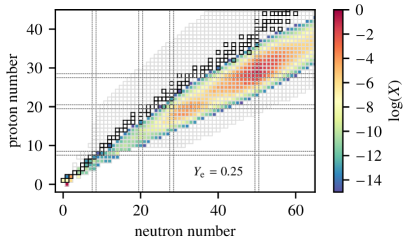
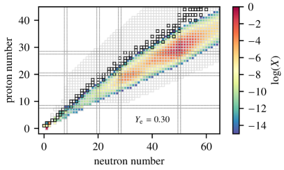
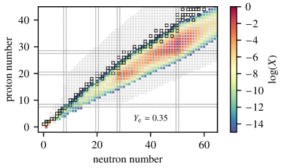
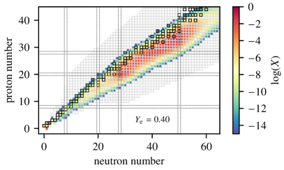
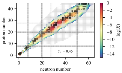
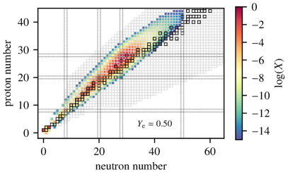
Figure 1: NSE distributions for varying electron fraction $Y_{\mathrm{e}}$ at $T=9$ GK and $\rho=10^{10}$ g cm^-3. The full reaction network is outlined in grey squares (it actually extends up to ²⁷⁶Bi with $Z=83$ and $N=193$). Stable isotopes are outlined in thicker, black squares. The vertical and horizontal dotted lines mark the magic neutron and proton numbers (shell closures) at 8, 20, 28 and 50.

These stellar evolution simulations are challenging, for a number of reasons. Firstly, super-AGB stars undergo several thousand thermal pulses (TPs; Ritossa et al., 1996; Siess, 2010; Jones et al., 2013; Doherty et al., 2015), in-between which the core increases very slowly in mass, at a rate of approximately $10^{-7}-10^{-6}\leavevmode\nobreak\ M_{\sun}\leavevmode\nobreak\ \mathrm{yr}^{-1}$. The rate of core growth depends crucially, however, on the efficiency, $\lambda$, of the third dredge-up (Herwig et al., 2012; Ventura et al., 2013; Jones et al., 2016a; Doherty et al., 2017). The thermal pulses themselves are the result of thermal instabilities in the He-burning shell, which is of the order of a mere $10^{-4}-10^{-5}\leavevmode\nobreak\ M_{\sun}$ of material (see, e.g. Ritossa et al., 1996, their Figure 15). Furthermore, the H burning shell resides inside the lower bound of the convective H envelope (hot bottom burning; Ventura & D’Antona, 2005a, b, 2011; Doherty et al., 2014). Resolving these phenomena for the entire evolution can require several hundreds of thousands, if not millions, of computational time steps in the stellar evolution calculation (Jones et al., 2013). Even then, the physics of convective boundary mixing during the TP-SAGB (CBM; Jones et al., 2016a) and the TP-SAGB wind mass loss rates are not known well enough (or modelled well enough; Groenewegen & Sloan, 2018) to accurately predict the dredge-up efficiency or the time at which the envelope would be completely expelled into the interstellar medium (Siess, 2007; Poelarends et al., 2008; Doherty et al., 2017). Understanding mass loss is further complicated by the fact that a substantial fraction of super-AGB stars are not isolated in space but exist in binary systems (Duchêne & Kraus, 2013) in which the companions will exchange mass during their lifetimes (Podsiadlowski et al., 2004; Sana et al., 2012; Tauris et al., 2015, 2017; Poelarends et al., 2017; Siess & Lebreuilly, 2018). At the upper end of this mass range, the evolution is challenging to model for different reasons. Most or all of the burning phases following C burning (that is, Ne, O and Si burning) ignite substantially away from the centre of the star and burn inwards as convectively bounded flames (Timmes et al., 1994; Jones et al., 2013; Woosley & Heger, 2015). These flames are typically not resolvable in stellar evolution calculations and so they tend to either burn inwards in some fashion influenced heavily by the numerical treatment, or they are quenched (perhaps somewhat artificially, e.g. Lecoanet et al., 2016) by mixing across them, induced by CBM from the bounding convection zone above (Jones et al., 2014). Simulating the evolution of the core during these events is also very time consuming and because the model depends on the numerical treatment, the accuracy is limited.

Another way of constraining the initial mass range for ECSNe would be to examine the observational statistics of their observable properties and compact remnants. In the case of a cECSN, the neutron stars produced are thought to have baryonic (gravitational) masses of around 1.35 $M_{\sun}$ (1.26 $M_{\sun}$; Schwab et al., 2010, e.g.). cECSN have similarities to the collapse produced when a white dwarf accretes sufficient matter to exceed the Chandrasekhar limit, also known as accretion induced collapse (AIC). Simulations of AICs predict remnant (gravitational) masses in the range $1.1-1.3\leavevmode\nobreak\ M_{\sun}$ (Hillebrandt et al., 1984; Baron et al., 1987; Fryer et al., 1999; Dessart et al., 2006; Abdikamalov et al., 2010). Both cECSN and AIC should produce similar compact remnant velocities. Because of the steep density profile, these systems produce explosions quickly. A number of mechanisms have been proposed to produce neutron star kicks (Fryer, 2004). If the remnant kick is produced through low-mode convection (that typically takes a longer timescale to develop), these systems will have low kick velocities (Herant, 1995; Fryer, 2004; Podsiadlowski et al., 2004; Knigge et al., 2011). If, instead, the kick is driven by asymmetries in the collapsing core, these systems will have strong kicks because convection will not have time to wash out the asymmetric collapse (Burrows & Hayes, 1996; Fryer, 2004).

Frustratingly, progenitors at the low-mass end of “regular” iron-core-collapse supernovae (FeCCSNe) also have relatively steep density gradients at the edge of the core, and similar core masses (Müller, 2016). Therefore it could be challenging to distinguish between neutron stars formed via cECSNe and those formed from the lower-mass end of the massive star mass range that explode as FeCCSNe.

Light curves of cECSNe from single stars are expected to be characterized by low peak bolometric luminosities and low ⁵⁶Ni ejecta masses compared to FeCCSNe from more massive FeCCSN progenitors with zero-age main sequence mass $M\gtrsim 12\leavevmode\nobreak\ M_{\sun}$. A number of such events have indeed been observed (e.g. Turatto et al., 1998; Botticella et al., 2009; Fraser et al., 2011; Kulkarni et al., 2007; Van Dyk et al., 2012) and reported as candidate cECSNe, but there are also theories that these optical transients are outbursts from massive stars (so-called supernova-impostors, e.g. Kulkarni et al., 2007; Bond et al., 2009; Berger et al., 2009) and not supernovae at all, or that they are FeCCSNe from massive stars in which there is a substantial amount of fallback, particularly of the ⁵⁶Ni (Turatto et al., 1998). In some cases candidate cECSN optical transients have even been ruled out as being exploding super-AGB stars (Eldridge et al., 2007).

Figure 2: Volume rendering showing the spatial distribution of electron fraction $Y_{\mathrm{e}}$ in the deflagration ashes of the $512^{3}$ ONe deflagration simulation G14.

Recently, Jerkstrand et al. (2018) published spectral synthesis results for the lowest-mass FeCCSN progenitor from Sukhbold et al. (2016) computed with the KEPLER stellar evolution code and exploded with the P-HOTB code in 1D (see Ugliano et al., 2012; Ertl et al., 2016; Sukhbold et al., 2016; Jerkstrand et al., 2018, for details). Jerkstrand et al. (2018) point out that of the three sub-luminous IIP SNe SN 1997D, SN 2005cs and SN 2008bk, all show He and C lines in their nebular spectra that are thought to originate from a thick He shell. This is consistent with massive star progenitors but not with super-AGB progenitors, adding weight to the interpretation of these three (and perhaps other) sub-luminous IIP SNe as being FeCCSNe from low-mass massive star progenitors and not cECSNe. Another low-luminosity IIP is SN 2016bkv, which does not exhibit the He and C lines associated with the He shell, but does still have O lines (Hosseinzadeh et al., 2018, their Figure 8), would be more consistent with a cECSN than SN 1997D, SN 2005cs or SN 2008bk, however its apparently large radioactive Ni ejecta mass is in tension with cECSN models. It cannot be ruled out, however, that the apparent enhancement of radioactive Ni in the ejecta of SN 2016bkv stems from an incomplete consideration of the CSM interaction in the modelling. There may still be life in the observational prospects of detecting ECSNe: super-AGB stars likely have low velocity winds with high mass loss rates, creating a dense circumstellar medium (CSM) around the star. Moriya et al. (2014) showed that because of this CSM, ECSNe would be of type IIn (H-rich but with narrow spectral lines from the slow-moving CSM), that may be consistent with the Crab supernova (Smith, 2013), which has been proposed to be the remnant of an ECSN.

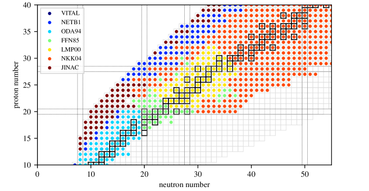
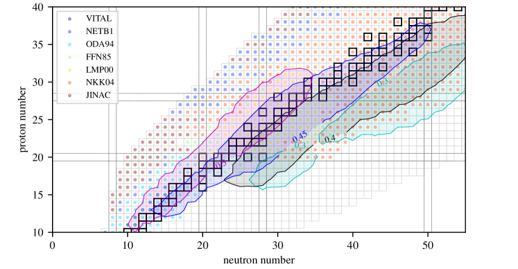
Figure 3: Top Panel: Sources of electron capture and positron decay ($\beta^{+}$) reaction rates in our reaction network. The labels are as follows: VITAL (only ${}^{7}\mathrm{Be}+\mathrm{e}^{-}\rightarrow^{7}\mathrm{Li}+\nu+\gamma$ from Caughlan & Fowler, 1988); NETB1 (weak reaction rates from NetGen – http://www.astro.ulb.ac.be/Netgen – which are predominantly from Takahashi & Yokoi, 1987 and Goriely, 1999); ODA94 (Oda et al., 1994); FFN85 (Fuller et al., 1985); LMP00 (Langanke & Martínez-Pinedo, 2000); NKK04 (Nabi & Klapdor-Kleingrothaus, 2004); JINAC (Cyburt et al., 2010). Bottom Panel: Same as top panel; shaded regions cover isotopes with mass fraction greater than $X=5\times 10^{-6}$ for an NSE state at $T=9$ GK and $\rho=10^{10}$ g cm^-3. The value of $Y_{\mathrm{e}}$ for each shaded region is written on the enclosing contour line. One can see that at $Y_{\mathrm{e}}=0.45$ there are a substantial number of isotopes outside of the region covered by the Langanke & Martínez-Pinedo (2000) tables with mass fractions greater than $X=5\times 10^{-6}$, indicating that they could potentially contribute to the evolution of $Y_{\mathrm{e}}$ when their weak reaction rates are considered, which is what we observe in our simulations when including the Nabi & Klapdor-Kleingrothaus (2004) rates.

If we continue down the path of not finding a transient or detecting a progenitor or a remnant that can unambiguously be identified as a smoking gun for a cECSN, then one must draw the conclusion that either (1) super-AGB stars never reach the conditions for explosion in isolated systems (i.e. not in an interacting binary); (2) that cECSNe are even less frequent than currently predicted, or (3) that our understanding of the explosion mechanism (and hence the synthetic observables, such as nucleosynthesis yields and light curves, spectra) is less complete than previously thought. This paper is an exploration of the possibility presented in point 3. Nomoto & Kondo (1991), Isern et al. (1991), Canal et al. (1992) and more recently Jones et al. (2016b) have suggested that there is a possibility that ECSNe could be thermonuclear explosions (i.e. exploding tECSNe rather than imploding cECSNe), as described above. Instead of collapsing into a neutron star, in a tECSN a portion of the core is ejected leaving a gravitationally bound WD remnant consisting of O, Ne and Fe-group elements (ONeFe WD) behind. It is these explosions that are the focus of this paper. There are two important predictions that can be used to constrain whether or not tECSNe can occur and at what frequency: the ejected material should contribute to galactic chemical evolution (GCE) and therefore to the solar chemical inventory, and the bound ONeFe WD remnants should still exist within our Galaxy. In both cases there are chemical signatures that are unique to these events owing to the extreme conditions under which the thermonuclear burning proceeds, compared to SNe Ia.

Building on the hydrodynamic tECSN simulations already performed by Jones et al. (2016b), we calculate the full nucleosynthesis in the ejecta and the bound remnant in the tECSN simulations. We also perform binary population synthesis simulations to obtain a theoretical estimate of the ECSN rate with respect to the FeCCSN rate should all ECSNe be tECSNe. We examine the nucleosynthesis results in the context of GCE, placing an upper limit on the frequency of occurrence of tECSNe by comparing to the solar abundance distribution. The composition of the ejecta is compared with recent measurements of pre-solar meteoritic oxide grains exhibiting extreme isotopic ratios for Cr and Ti, for which tECSNe are found to be a remarkably good match. Lastly, we compute mass-radius relations for the bound ONeFe WD remnants and compare them with both the population synthesis results and observational WD surveys.

It is worth re-emphasizing at this point that we believe the outcome of ECSNe – cECSN, implosion and NS or tECSN, explosion and ONeFe WD – remains an open question at present. This is because obtaining a convincing answer using simulations depends on several modelling assumptions and microphysics constraints, as described by Jones et al. (2016b). Additionally, the ignition density of the deflagration remains uncertain, which is critical input for the hydrodynamic simulations. We hope that this study of the nucleosynthesis and compact remnants in the case of a partial thermonuclear explosion brings us closer to an answer.

2 Post-processing technique and reaction network

2.1 Nuclear reaction network: approach and methods

The simulations presented in Jones et al. (2016b) included the advection of $\sim 10^{6}$ equal-mass tracer particles, as has been described in several previous works (Travaglio et al., 2004; Röpke et al., 2006; Seitenzahl et al., 2010, 2013b). In this work, we performed nucleosynthesis simulations of these tracer particles in post-processing, taking the temperature and density evolution of the tracer particles as a function of time and integrating the reaction equations for those conditions. For the post-processing, a derivative of the NuGrid nuclear reaction network was used (as has briefly been described in Pignatari et al., 2016; Ritter et al., 2018). The network was substantially renovated and updated to use the screening corrections for fusion reactions by Chugunov et al. (2007) and the semi-implicit extrapolation method by Bader & Deuflhard (1983) and Deuflhard (1983) was implemented (see also Timmes, 1999), which was used for all simulations presented here. A new nuclear statistical equilibrium (NSE) solver was also written largely following the work of Seitenzahl et al. (2009), and the NSE state solution at a given $(T,\rho,Y_{\mathrm{e}})$ is now coupled to the weak reactions (for the time-dependence of the electron fraction $Y_{\mathrm{e}}$) using a Cash-Karp type Runge-Kutta integrator (Cash & Karp, 1990). Reverse reaction rates were computed in real time from their forward rates using the principle of detailed balance (see the appendix of Calder et al., 2007, for a concise formulation). This improved the agreement between the reaction network and the NSE solver. The network dynamically adapts the problem size at every integration step in order to minimize the computational cost of the matrix inversion that must be performed at least twice per time step (i.e. for the first two levels of the Bader-Deuflhard integrator with $n=2$ and $n=6$). The matrix is written directly into a sparse format, after which it is compressed down to the problem size for the time step and the LU decomposition and subsequent back-substitutions are then performed using the SuperLU sparse matrix library (Demmel et al., 1999; Li et al., 1999; Li, 2005) together with the OpenBLAS BLAS library.

The abundance distributions were post-processed for a second time to account for the radioactive decay of the ejecta following the explosion. Only spontaneous decays occur in the cold, low density environment of the ejecta. The decay rates were assumed to be the same as under terrestrial conditions where many experimental data exist. The decays of isotopes with mass fractions $>10^{-20}$ were processed with a relative uncertainty of better than 1 %.

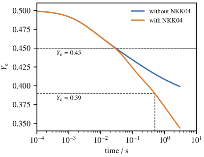
Figure 4: Evolution of electron fraction $Y_{\mathrm{e}}$ in a constant temperature and density network integration with and without the weak rates by Nabi & Klapdor-Kleingrothaus (2004) included in the reaction network at their positions from Figure 3. The conditions were $T=9$ GK, $\rho=10^{10}$ g cm^-3 and $Y_{\mathrm{e}}(t=0)=0.5$. The two curves separate below $ye\approx 0.45$, where the contribution of the fp and fpg shell nuclei to the deleptonization become significant.

2.2 Neutron-richness in thermonuclear explosions

Before we construct a nuclear reaction network and choose a suitable set of reaction rates, we first explore the conditions under which nucleosynthesis occurs in tECSNe. Although the physical mechanism is similar to thermonuclear explosions in CO white dwarfs, we find that the reaction networks used in these studies (Travaglio et al., 2004; Röpke et al., 2005; Seitenzahl et al., 2010) are insufficient for our models.

While in the context of Type Ia supernova explosion models two modes for the propagation of thermonuclear combustion fronts are discussed – subsonic deflagrations and supersonic detonations (see, e.g. Röpke, 2017) – our models of electron capture supernovae assume burning to proceed in the subsonic deflagration regime exclusively. The burning products by the deflagration in high density ONe cores or WDs can generally be well described by nuclear statistical equilibrium (see, e.g. Seitenzahl et al., 2009). That is, the timescale for the strong reactions to equilibrate is shorter than the timescale on which the local thermodynamic conditions of the material are changing. In this case, that is the hydrodynamic time-scale. The weak reaction rates (electron/positron-captures and $\beta^{\pm}$-decays) for the prevalent isotopes are typically much slower than the strong reactions and can not necessarily be assumed to reach equilibrium.

The isotopic composition of material in NSE depends critically on $Y_{\mathrm{e}}$. Figure 1 shows six pseudo-colour plots of the isotopic nuclear chart, where the colour scale represents the mass fractions of the isotopes for NSE solutions with $T=9$ GK, $\rho=10^{10}$ g cm^-3 (i.e. a typical state that is reached in a tECSN) and $Y_{\mathrm{e}}=\{0.25,0.3,0.35,0.4,0.45,0.5\}$. It is relatively well-known that the NSE distribution will tend to favour nuclei with a ratio of proton number to mass number $Z/A\approx Y_{\mathrm{e}}$ (e.g. Clifford & Tayler, 1965; Hartmann et al., 1985), which can be seen in the most abundant (red) isotopes in Figure 1, which tend to more neutron-rich nuclei for lower $Y_{\mathrm{e}}$. It is interesting that in Figure 1 one can clearly see the bifurcation of the peak NSE distribution (aside from the free nucleons) at lower values of electron fractions, with the two peaks staying close to the intersection of the magic neutron and proton numbers at $Z=\{20,28\}$ and $N=\{28,50\}$.

The values of $Y_{\mathrm{e}}$ reached in models for Type Ia supernova explosions depend on the metallicity of the progenitor star and its central density. The most massive Type Ia supernova progenitors are postulated to be degenerate CO white dwarf stars with masses at the Chandrasekhar limit, which for a non-rotating CO white dwarf star would be close to $1.4\leavevmode\nobreak\ M_{\odot}$. It has been argued that differential rotation can substantially increase the mass supported against collapse (Steinmetz et al., 1992; Pfannes et al., 2010b, a) and some observed superluminous Type Ia supernovae have been associated with explosions of progenitors with masses above $1.4\leavevmode\nobreak\ M_{\odot}$ (e.g. Howell et al., 2006; for an overview see Taubenberger, 2017), but burning is not expected to take place at extremely high densities in these scenarios and the results are inconsistent with observed supernovae (Fink et al., 2018). One widely discussed scenario for normal Type Ia supernovae is that a thermonuclear runaway of C in Chandrasekhar-mass WDs initiates a deflagration wave that almost immediately enters the turbulent burning regime and later may or may not transition into a detonation (delayed detonation model, Khokhlov, 1991). While a pure turbulent deflagration is a successful model for the subluminous class of SN 2002cx-like Type Ia supernovae (e.g. Kromer et al., 2013), three-dimensional simulations of the delayed detonation scenario reproduce many of the observational characteristics of Type Ia supernovae (e.g. Kasen et al., 2009; Blondin et al., 2013), but fail in some (important) aspects (Sim et al., 2013). The highest density that can be achieved in a Chandrasekhar-mass Type Ia supernova explosion is the initial central density of the progenitor, which is about $\rho_{\mathrm{c}}\approx 2-5\times 10^{9}$ g cm^-3 for an appropriate value of the electron fraction in the CO white dwarf (Lesaffre et al., 2006), depending on its cooling history. At these densities, the deflagration ashes will be buoyant (high Atwood number), resulting in substantial expansion of the CO white dwarf of the order of a few hundred milliseconds, together with a corresponding decrease in the maximum density. On the time-scale of a few hundred milliseconds the deleptonization of the densest material in a CO white dwarf proceeds only at a moderate rate and $Y_{\mathrm{e}}$ typically does not fall below about 0.46 (e.g. Travaglio et al., 2004).

Conversely, in the ONe deflagration during an ECSN the Atwood number is substantially lower than in a Type Ia SN owing to the higher densities and the higher degree of electron degeneracy. The densest regions expand more slowly and spend more time at densities where the rate of deleptonization is much faster. If the deleptonization is fast enough and the Atwood number is low enough, the ONe WD or the degenerate ONe core will experience a rapid decrease in $Y_{\mathrm{e}}$ and the core will eventually collapse into a neutron star (Miyaji et al., 1980; Nomoto, 1987; model H01 of Jones et al., 2016b). In less extreme cases (i.e. lower central densities of the ONe core at the time of deflagration ignition; $\rho_{c}\lesssim 10^{10}$ g cm^-3), the nuclear energy released may compete with the deleptonization and the buoyant acceleration of the hot ashes can lead to the unbinding of a substantial fraction of the core. For such a case, the minimum $Y_{\mathrm{e}}$ found in simulations is $Y_{\mathrm{e}}\sim 0.38$ (Figure 2 and Jones et al., 2016b, their Figure 2).

Table 1: Isotopes included in the post-processing reaction network.

element	min. $A$	max. $A$
n	1	1
H	1	3
He	3	6
Li	7	9
Be	7	12
B	8	14
C	11	18
N	11	21
O	13	22
F	17	26
Ne	17	41
Na	19	44
Mg	20	47
Al	21	51
Si	22	54
P	23	57
S	25	60
Cl	26	63
Ar	27	67
K	29	70
Ca	30	73

element	min. $A$	max. $A$
Sc	32	76
Ti	34	80
V	36	83
Cr	38	86
Mn	40	89
Fe	42	92
Co	44	96
Ni	46	99
Cu	48	102
Zn	51	105
Ga	53	108
Ge	55	112
As	57	115
Se	59	118
Br	61	121
Kr	63	124
Rb	66	128
Sr	68	131
Y	70	134
Zr	72	137
Nb	74	140

element	min. $A$	max. $A$
Mo	77	144
Tc	79	147
Ru	81	150
Rh	83	153
Pd	86	156
Ag	88	160
Cd	90	163
In	92	166
Sn	94	169
Sb	97	172
Te	99	176
I	101	179
Xe	103	182
Cs	106	185
Ba	108	189
La	110	192
Ce	113	195
Pr	115	198
Nd	118	201
Pm	120	205
Sm	123	208

element	min. $A$	max. $A$
Eu	125	211
Gd	128	214
Tb	130	218
Dy	133	221
Ho	136	224
Er	138	227
Tm	141	230
Yb	143	234
Lu	146	237
Hf	149	240
Ta	151	243
W	154	247
Re	156	250
Os	159	253
Ir	162	256
Pt	165	260
Au	167	263
Hg	170	266
Tl	173	269
Pb	175	273
Bi	178	276

2.3 Nuclear reaction network: species and rates

Owing to the extreme conditions encountered in our models, we have to extend the nuclear reaction network beyond the isotopes and rates usually accounted for in post-processing thermonuclear supernova explosion models. For these simulations, we simply used the largest pool of nuclei available in our reaction network, which is 5234. The bounds of the network on the neutron- and proton-rich sides are determined by comparing the $\beta^{\pm}$-decay half lives of the isotopes with a user-defined minimum characteristic time for the problem at hand. The network is closed at the boundaries by “ghost” isotopes that are forced to instantaneously $\beta^{\pm}$-decay (depending upon whether they are proton-rich or neutron-rich). For our problem we set the minimum characteristic time to $10^{-5}$ seconds. After establishing the boundaries of the network from this time-scale, we are left with a total of 5213 isotopes in the network proper (see Table 2.2). This is almost certainly too large a network for the problem at hand, however as one can see in Figure 1 – in which the isotopes included in the network are drawn in grey squares – in NSE at the lowest $Y_{\mathrm{e}}$ (0.25), there are moderately abundant isotopes only a handful of neutrons away from the edge of the network on the neutron-rich side. Similarly, at $Y_{\mathrm{e}}=0.5$, there are moderately abundant isotopes only a handful of protons away from the edge of the network on the proton-rich side. One can also see in Figure 1 that in NSE at lower $Y_{\mathrm{e}}$ there is more material with higher $A$, necessitating that the network extend well above $A=100$. In order not to artificially influence our results by hitting the network boundaries, we did not attempt to make the network any smaller, although there are ways in which this could have been done. From a practical standpoint, the motivation to reduce the network size originates from a desire to also reduce the computational cost of the simulation. However, the nuclear reaction network is designed to perform the time-integration at each time step only for a sub-set of isotopes whose abundances are actually changing. This means that all of the matrix inversions and back-substitutions are much cheaper than if we were to perform them for the complete set of 5213 isotopes every time step. In order to determine which isotopes should be included in the solve each time step, we do still need to evaluate all of the reaction rates for all of the isotopes in the network, which does come with an additional and perhaps somewhat avoidable computational cost.

The reaction rates in the network were taken from JINA Reaclib (Cyburt et al., 2010), KaDoNiS (Dillmann et al., 2006), NACRE (Angulo et al., 1999) and NON-SMOKER (Rauscher & Thielemann, 2000), as well as from Fuller et al. (1985), Takahashi & Yokoi (1987), Goriely (1999), Langanke & Martínez-Pinedo (2000), Iliadis et al. (2001) and Oda et al. (1994). There are also a handful of reactions whose rates have been individually selected from the literature, including from Caughlan & Fowler (1988) for several reactions, Jaeger et al. (2001) for the ${}^{22}\mathrm{Ne}(\alpha,n)^{25}\mathrm{Mg}$ reaction, Imbriani et al. (2005) for the ${}^{14}\mathrm{N}(p,\gamma)^{15}\mathrm{O}$ reaction, several proton capture reactions from Champagne & Wiescher (1992), Fynbo et al. (2005) for ${}^{4}\mathrm{He}(2\alpha,\gamma)^{12}\mathrm{C}$, Kunz et al. (2002) for ${}^{12}\mathrm{C}(\alpha,\gamma)^{16}\mathrm{O}$, Heil et al. (2008) for ${}^{13}\mathrm{C}(\alpha,n)^{16}\mathrm{O}$ and Rauscher et al. (1994) for ${}^{17}\mathrm{O}(n,\alpha)^{14}\mathrm{C}$. Several of the $(n,\gamma)$ reactions have been updated from the KaDoNis release and have been listed in Denissenkov et al. (2018, footnote 13). We also made use of the NUDAT Nuclear data files provided by the National Nuclear Data Center (NNDC; Kinsey et al., 1996). Nuclear masses and partition funtions are as provided by the JINA Reaclib database, and are used in the NSE solver and for calculating reverse reaction rates.

Given that the majority of the burning takes place under conditions where assuming NSE is appropriate, we paid special care to the weak reaction rates. The top panel of Figure 3 shows the sources of electron-capture and $\beta^{+}$-decay rates that we use in the reaction network. The bottom panel of Figure 3 shows the same information as the top panel but has a portion of the information about the NSE distributions from Figure 1 overlaid. More specifically, it shows shaded contours enclosing regions of the isotopic chart where the isotopic mass fractions are greater than $5\times 10^{-6}$ in an NSE state for $T=9$ GK, $\rho=10^{10}$g cm^-3 and $Y_{\mathrm{e}}=\{0.3,0.4,0.45,0.5\}$. Already at $Y_{\mathrm{e}}=0.45$ (approximately the minimum $Y_{\mathrm{e}}$ reached in standard type Ia SNe) there are isotopes with relatively large mass fractions that lie outside of the pf shell and are therefore quite inaccessible to nuclear shell-model codes. Nevertheless, there is a possibility that these isotopes can collectively contribute to the overall rate of (de)leptonization in the star. Weak reaction rate tables for a large pool of nuclei were computed and made available by Juodagalvis et al. (2010), however they included only electron-capture and $\beta^{+}$-decay reactions and did not include their inverses. This omission is likely inconsequential if modelling FeCCSNe, however having an as-accurate-as-possible balance of the forward and reverse rates is necessary for ECSNe when one is attempting to determine whether the situation resolves in core collapse or not. We have opted to use the reaction rates from the quasiparticle random phase approximation (QRPA) calulations by Nabi & Klapdor-Kleingrothaus (2004) for fp and fpg shell nuclei because of their extensive coverage of the isotopic chart and the fact that reaction rates have been computed for both directions. Even so, at $Y_{\mathrm{e}}=\{0.3,0.4\}$ there are still a handful of isotopes with mass fractions greater than $5\times 10^{-6}$ (i.e. within the shaded regions in Figure 3, bottom panel) for which we do not have electron-capture or $\beta^{+}$-decay reaction rates.

The impact of the additional weak reaction rates by Nabi & Klapdor-Kleingrothaus (2004) is shown in Figure 4 for a network integration at constant temperature ($9$ GK) and density ($10^{10}$ g cm^-3) and initial $Y_{\mathrm{e}}(t=0)=0.5$. The $Y_{\mathrm{e}}$ evolution with and without the NKK reaction rates clearly diverge below $Y_{\mathrm{e}}\approx 0.45$, as discussed earlier in this Section. We also mentioned that the minimum $Y_{\mathrm{e}}$ achieved in the sub-set of partially exploding (i.e. not collapsing) simulations by Jones et al. (2016b) was 0.39. This $Y_{\mathrm{e}}$ has been marked on Figure 4 in a manner illustrating that this $Y_{\mathrm{e}}$ is reached after 0.5 seconds under these conditions. This is intuitive because the dynamical time-scale of an ONe white dwarf with a central density of $10^{10}$ g cm^-3 is indeed about 0.5 seconds.

Table 2: Relevant properties of the hydrodynamic simulations from Jones et al. (2016b). Only the models that are tECSNe are shown. In order from left to right, the columns are: model id, grid resolution, Coulomb corrections included in EoS (Y/N), central density at ignition of the deflagration, bound ONeFe remnant mass, mass of the ejected material, average electron fraction in the ONeFe remnant, and mass fraction of iron-group elements in the ONeFe remnant. The model J07 is a new addition. Nucleosynthesis simulations have been performed for models G14 and J07, which were used for this work.

id	res	CCs	$\log_{10}\rho_{\mathrm{c}}^{ini}$	$M_{\mathrm{rem}}$	$M_{\mathrm{ej}}$	$\langle Y_{\mathrm{e}}\rangle$	$X_{\mathrm{IGE}}$
			(g cm-3)	($M_{\odot}$)	($M_{\odot}$)
G13	$256^{3}$	N	9.90	0.647	0.741	0.491	0.267
G14	$512^{3}$	N	9.90	0.438	0.951	0.491	0.263
G15	$256^{3}$	Y	9.90	1.212	0.177	0.493	0.184
J01	$256^{3}$	N	9.95	0.631	0.768	0.491	0.271
J02	$256^{3}$	Y	9.95	1.291	0.104	0.493	0.175
J07	$576^{3}$	N	9.95	0.366	1.027	0.489	0.293

2.4 Input from hydrodynamic simulations

In Jones et al. (2016b), we performed 3d hydrodynamic simulations of deflagration fronts in ONe WDs with a range of plausible ignition densities (we will use the terminology ONe deflagrations to describe this scenario). Within the set of six models, there were five models that resulted in a partial ejection (gravitational unbinding) of material, leaving behind a gravitationally bound ONeFe WD (tECSNe). One model – with the highest central density at ignition, $2\times 10^{10}$ g cm^-3 – collapsed into a neutron star. Of the five models that were tECSNe, two included a correction to the internal energy and pressure in the equation of state (EoS) from the non-ideal behaviour of the plasma (Coulomb corrections; CCs).

The relevant results from Jones et al. (2016b) are summarized in Table 2 for convenience. This paper is concerned only with the nucleosynthesis in the tECSNe and therefore the model H01 has been omitted. We note that we have added a new hydrodynamic simulation J07 to this work, which is a higher-resolution version of J01 from Jones et al. (2016b). We added this model because we would like to compare the nucleosynthesis in models with different ignition densities at a similar (and as high as possible) numerical resolution. For this work we will therefore be using simulations G14 and J07. To re-state a pertinent point from Jones et al. (2016b): although our simulations do not yet exhibit convergence upon grid refinement, increasing the grid resolution yields a higher ejected mass, suggesting that further increasing the grid resolution will likely keep the outcome as a tECSN and not a core-collapse. Nevertheless, we admit that there is still much to do to improve the status of the hydrodynamic simulations, and this is currently a work in progress.

In each of the hydrodynamic simulations, a set of $\sim 10^{6}$ Lagrangian tracer particles were passively advected with the flow, sampling their local thermodynamic environment. As a result, we obtain a trajectory for each particle, which contains temperature and density as a function of time. The method for assigning the tracer particle masses and initial spatial distribution was the same as in Seitenzahl et al. (2010), which we briefly summarize here for convenience, but to which we refer the interested reader for complete details. The tracer particle masses vary smoothly with initial radius and their distribution is broken into three spatial parts. Within some radius $R_{1}$ the tracer particles have equal mass and resolve the region where the density profile is relatively flat and most of the NSE burning takes place. For initial radii $R_{1}<R<R_{2}$, where the density gradient is steeper and the density is lower, the tracer particles have equal volume and therefore provide better sampling of the lower density material where incomplete burning synthesizes intermediate-mass elements (IMEs). Lastly, the particles in the exterior layer with initial radii $R>R_{2}$ have equal mass again. To compute the nucleosynthesis, the particle trajectories were fed directly into the post-processing network for each particle at the time when the deflagration front arrives at that particle’s location.

3 Nucleosynthesis results

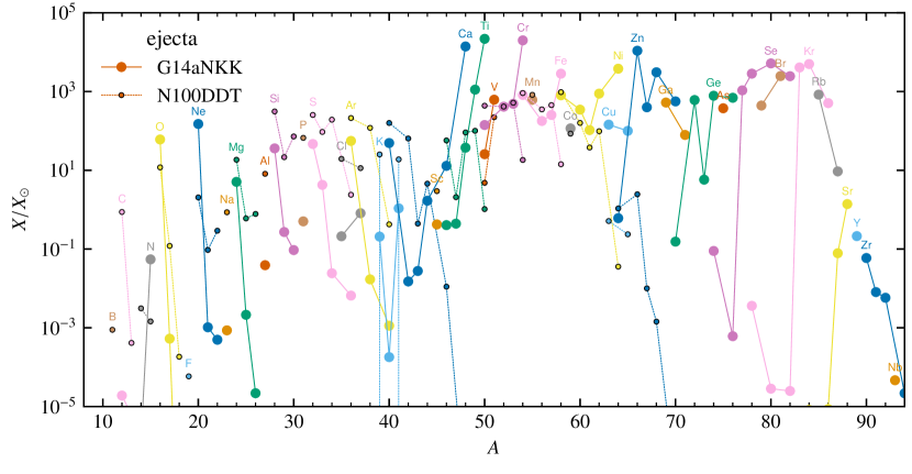
Figure 5: Overabundance (mass fraction relative to solar; $X/X_{\odot}$) of stable isotopes in the ejecta of simulation G14aNKK after decaying for $10^{16}$ s (0.32 Gyr). The striking production of ${}^{48}\mathrm{Ca}$, ${}^{50}\mathrm{Ti}$ and ${}^{54}\mathrm{Cr}$ is a partcular hallmark of deflagrations in degenerate media high-density (see, e.g. Woosley, 1997). The DDT simulation N100DDT from Seitenzahl et al. (2013b) is plotted for comparison, decayed to 2 Gyr.

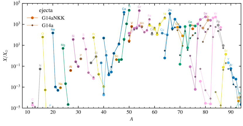
Figure 6: Overabundance (mass fraction relative to solar; $X/X_{\odot}$) of stable isotopes in the ejecta of simulation G14a after decaying for $10^{16}$ s. The two lines correspond to post-processing nucleosynthesis simulations where Nabi & Klapdor-Kleingrothaus (2004, NKK) weak reaction rates were included (”NKK”) and when they were not. Including the NKK rates results in a larger yield of ${}^{48}\mathrm{Ca}$ and smaller yields of ${}^{50}\mathrm{Ti}$ and ${}^{54}\mathrm{Cr}$. The yields of the trans-iron elements from Ga to Nb are substantially increased when the NKK rates are included.

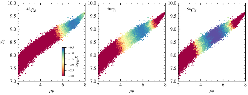
Figure 7: Mass fractions of ${}^{48}\mathrm{Ca}$, ${}^{50}\mathrm{Ti}$ and ${}^{54}\mathrm{Cr}$ as a function of peak temperature (GK) and density ($\rho_{9}=10^{9}$ g cm^-3) for the sub-set of tracer particles where these isotopes are made in abundance.

The nucleosynthesis in the ejecta of our ONe deflagration simulations is, rather unsurprisingly, very similar to the nucleosynthesis in the high density CO deflagration simulations by Woosley (1997). The overabundances (mass fractions relative to solar) of the stable nuclei after the ejecta has been allowed to decay for $10^{16}$ s are shown in Figure 5. Also shown for reference in Figure 5 is model N100DDT from Seitenzahl et al. (2013b), that follows a delayed detonation in a Chandrasekhar-mass CO white dwarf star. It is noteworthy that these are of course mass fractions, and the total ejecta of N100DDT is roughly 50% more massive than G14a. The four main distinguishing features of the ONe deflagration compared with N100DDT are: (1) substantial deficit of C; (2) ejection of large quantities of O and Ne from the progenitor; (3) presence of a very large (relative to solar) quantity of trans-iron elements from Zn to Rb, and (4) significant overproduction of ${}^{48}\mathrm{Ca}$, ${}^{50}\mathrm{Ti}$ and ${}^{54}\mathrm{Cr}$, again relative to solar. Observations 1 and 2 are perhaps obvious, and the remaining points have already been identified and published in the context of high density CO deflagrations by Woosley (1997), and so in this sense what we present here could be conveyed as not particularly novel. However, there are two aspects of our work that build on Woosley (1997): (a) the existence of ONe WDs with such extreme central densities is supported by stellar evolution theory (whereas there is no clear plausible formation channel for CO WDs with densities as high as $8\times 10^{9}$ g cm^-3), and (b) weak reaction rates for the fp- and fpg-shell neutron-rich iron-group isotopes are now available.

Woosley concluded that given there was no other compelling site for producing ${}^{48}\mathrm{Ca}$, exotic high density CO deflagrations must occasionally occur, at about 2% of the “normal” type Ia SN rate. However, it is not completely clear how such a high density CO white dwarf could be formed without burning C into O and Ne and transforming into an ONe white dwarf. One opportunity would be in the merger of two CO white dwarf stars, but those are expected to either explode during the merging process (e.g. Pakmor et al., 2012) or also transform into an ONe white dwarf and then a Si white dwarf, or burning proceeds through to Fe-group elements and the core collapses into a neutron star (see, e.g., Saio & Nomoto, 1985; Nomoto & Iben, 1985; Schwab et al., 2016). Our paper proposes a possible solution to this conundrum in which massive CO white dwarfs well above the critical mass for carbon ignition and ONe white dwarf formation do not have to exist. We, of course, are plagued by other, different questions and uncertainties such as whether or not the conditions of ONe cores at ignition are favourable for a partial thermonuclear explosion. If they indeed all collapse, neither do we have a solution. It should be mentioned, however, that since Woosley’s work in 1997, Wanajo et al. (2013a) found that ${}^{48}\mathrm{Ca}$ can also be produced in ECSNe in the case where they collapse into a neutron star. The yields from the cECSN simulations from Wanajo et al. (2013a, b) are given in the last column of Table 3, for comparison with our simulation results for tECSNe (G14 and J07). Per event, our tECSN simulations produce about $2\times 10^{-3}\leavevmode\nobreak\ M_{\sun}$ of ${}^{48}\mathrm{Ca}$ (ejecta mass is approximately 1 $M_{\sun}$) while the cECSN simulations by Wanajo et al. (2013a, b) produce about $2\times 10^{-5}\leavevmode\nobreak\ M_{\sun}$ – 2 orders of magnitude less.

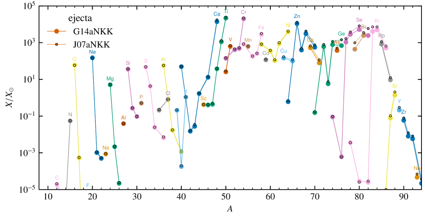
Figure 8: Same as Figures 5 and 6 but comparing two simulations with different initial central densities. G14a is the $512^{3}$ simulation from Jones et al. (2016b) with initial central density $\log_{10}(\rho/\mathrm{g\leavevmode\nobreak\ cm}^{-3})=9.9$ and J07a is a $576^{3}$ resolution version of simulation J01 from Jones et al. (2016b), which had an initial central density of $\log_{10}(\rho/\mathrm{g\leavevmode\nobreak\ cm}^{-3})=9.95$. The higher density simulation exhibits an ejecta that is moderately enhanced in the neutron-rich isotopes and the trans-iron elements (see also Table 2 and Table 3).

Table 3: Mass fractions of stable isotopes or elements of interest from the solar distribution (Asplund et al., 2009), the W7 type Ia SN model (Nomoto et al., 1984), the N100DDT type Ia SN model (Seitenzahl et al., 2013b), and the G14a ONe deflagration simulation (Jones et al., 2016b), with and without weak reaction rates by Nabi & Klapdor-Kleingrothaus (2004) included in the nucleosynthesis post-processing. The higher-density model J07 is also included (see Table 2). The last column is the cECSN yields from Wanajo et al. (2013a, b), where the total ejecta mass was $1.14\times 10^{-2}\leavevmode\nobreak\ M_{\sun}$. The simulation results are all decayed yields, i.e. they are for the ejecta only. The N100DDT model was decayed to 2 Gyr and the G14 and J07 models to $10^{16}$ s (enough time for all radioactive nuclides produced to decay – see half lives in Table 4.

isotope/element	$\odot$	W7	N100DDT	G14a	G14aNKK	J07aNKK	W13
Zn	1.85e-06	2.06e-05	2.22e-06	4.83e-03	6.80e-03	8.33e-03	9.97e-02
Se	1.34e-07	0.00e+00	0.00e+00	4.51e-05	4.80e-04	7.60e-04	6.87e-03
Kr	1.16e-07	0.00e+00	0.00e+00	4.41e-05	3.95e-04	5.86e-04	1.04e-02
${}^{48}\mathrm{Ca}$	1.53e-07	1.90e-09	5.60e-15	1.32e-03	2.13e-03	2.64e-03	2.04e-03
${}^{50}\mathrm{Ti}$	1.79e-07	7.82e-05	1.86e-07	4.46e-03	3.91e-03	4.37e-03	1.65e-04
${}^{54}\mathrm{Cr}$	4.33e-07	6.75e-04	7.92e-06	9.48e-03	8.64e-03	9.56e-03	3.97e-04

Table 4: Ejected masses of radioactive isotopes in the N100DDT type Ia SN model (Seitenzahl et al., 2013b), and the G14aNKK ONe deflagration simulation (Jones et al., 2016b) ejecta at 100 s after ignition. Isotopes with half lives less than $10^{4}$ s have been omitted.

isotope	N100DDT	G14aNKK	half life / s
56Ni	6.04e-01	1.87e-01	5.25e+05
57Ni	1.79e-02	6.00e-03	1.28e+05
66Ni		5.37e-03	1.97e+05
55Co	1.14e-02	4.45e-03	6.31e+04
60Fe	4.20e-10	2.81e-03	8.27e+13
52Fe	7.93e-03	2.42e-03	2.98e+04
55Fe	1.86e-03	1.48e-03	8.66e+07
57Co	8.70e-04	6.85e-04	2.35e+07
59Ni	3.93e-04	2.65e-04	2.40e+12
53Mn	2.35e-04	1.72e-04	1.18e+14
62Zn	3.22e-04	1.36e-04	3.31e+04
56Co	1.18e-04	8.78e-05	6.67e+06
48Cr	3.14e-04	8.63e-05	7.76e+04
59Fe	2.72e-09	5.26e-05	3.84e+06
72Zn		3.98e-05	1.67e+05
63Ni	1.76e-08	2.59e-05	3.19e+09
67Cu		2.00e-05	2.23e+05
77Ge		9.99e-06	4.04e+04
54Mn	3.03e-06	7.57e-06	2.70e+07
58Co	4.35e-06	4.18e-06	6.12e+06
51Cr	9.29e-06	3.59e-06	2.39e+06
44Ti	9.98e-06	2.50e-06	1.87e+09
52Mn	5.18e-06	2.12e-06	4.83e+05
37Ar	3.43e-05	1.70e-06	3.02e+06
60Co	2.03e-08	1.10e-06	1.66e+08
61Cu		9.58e-07	1.20e+04
85Kr		4.03e-07	3.39e+08
41Ca	6.07e-06	2.36e-07	3.14e+12
73Ga		7.06e-08	1.75e+04
47Ca		6.69e-08	3.92e+05
49V	3.57e-07	5.01e-08	2.85e+07
88Kr		4.98e-08	1.02e+04
48V	9.12e-08	4.41e-08	1.38e+06
77As		4.35e-08	1.40e+05
22Na	4.27e-09	4.10e-08	8.21e+07
26Al	5.68e-07	2.42e-08	2.26e+13
79Se		2.02e-08	1.03e+13
45Ti		1.97e-08	1.11e+04
64Cu		3.86e-09	4.57e+04
48Sc		3.56e-09	1.57e+05
43Sc		2.60e-09	1.40e+04
47Sc		2.36e-09	2.89e+05
90Sr		7.32e-10	9.09e+08
65Zn	7.35e-10	3.65e-10	2.11e+07
66Ga		3.39e-10	3.42e+04
68Ge	6.33e-10	1.91e-10	2.34e+07
89Sr		1.06e-10	4.37e+06
36Cl	7.77e-07	1.03e-11	9.51e+12
33P	3.76e-07	9.77e-12	2.19e+06
32Si	9.47e-09	7.32e-12	4.83e+09
35S	5.39e-07	3.04e-12	7.55e+06
32P	4.96e-07	1.97e-12	1.23e+06
40K	5.81e-08	9.99e-13	3.94e+16
39Ar	1.29e-08	3.17e-13	8.49e+09
14C	2.47e-06	6.49e-17	1.80e+11

We were fortunate enough to have access to the QRPA calculations by Nabi & Klapdor-Kleingrothaus (2004) for the fp and fpg shell nuclei on the neutron-rich side of the valley of stability, which were not available in 1997 when Woosley conducted his study of deflagrations in high-density CO white dwarfs. It is worth also mentioning that many of the reaction rates that we have used originate from more recent measurements or calculations than those used by Woosley (1997). Of particular note are the weak reaction rates for the pf shell nuclei by Langanke & Martínez-Pinedo (2000). Woosley (1997) commented that at some point when weak reaction rates for the fp and fpg shell nuclei became available, it would be of some interest to study how their inclusion could change the nucleosynthesis yields from deflagrations in high-density CO white dwarfs. We have indeed done this, but for high density ONe white dwarfs. We expect that the outcome is probably very similar whether the fuel is CO or ONe, because (a) the binding energy (relative to free nucleons) of ¹²C is similar to ²⁰Ne, i.e. $7.41\times 10^{18}$ erg g^-1 for ¹²C and $7.75\times 10^{18}$ erg g^-1 for ²⁰Ne (numbers are relative to free nucleons) and (b) because for both CO and ONe white dwarfs, at least 50% of the mass is ususally ¹⁶O. In fact, the binding energy of ¹⁶O is $7.70\times 10^{18}$ erg g^-1 (99% that of ²⁰Ne), meaning that an ONe white dwarf is very similar indeed to a CO white dwarf with a low C/O ratio.

The impact of including the NKK04 reaction rates in the post-processing nucleosynthesis simulation of model G14a is shown in Figure 6. As we have shown in Figure 4, including the NKK04 rates results in faster deleptonization at high densities than when they are omitted. We also showed in Figure 1 that with decreasing $Y_{\mathrm{e}}$ (for fixed $T,\rho$), the NSE distribution solution favours not only more neutron-rich nuclei, but nuclei with higher atomic weight, than at higher $Y_{\mathrm{e}}$. This effect is evident in Figure 6 in the extra production of the trans-iron elements between Zn and Sr. Although the changes may not look like much in Figure 6, because of the logarithmic scale, the enhancement of the elemental abundances of both Se and Kr are about 1 dex when the NKK04 rates are included (see Table 3). The ${}^{48}\mathrm{Ca}$ yield increases by 61%, the Zn yield increases by 41% and the yields of ${}^{50}\mathrm{Ti}$ and ${}^{54}\mathrm{Cr}$ decrease by 12% and 8.9%, respectively. The final mass fractions of ${}^{48}\mathrm{Ca}$, ${}^{50}\mathrm{Ti}$ and ${}^{54}\mathrm{Cr}$ for the tracer particles in the G14 simulation experiencing the most extreme conditions are shown as a function of the peak temperature and peak density in Figure 7.

Also shown in Table 3 are the mass fractions of these isotopes and elements in the ejecta of simulation J07a (final column). This simulation is a $576^{3}$ version of the simulation J01 from Jones et al. (2016b), which had an initial central density of $\log_{10}(\rho/\mathrm{g\leavevmode\nobreak\ cm}^{-3})=9.95$, compared to $9.9$ for G14a. One can see from the comparison in Figure 8 that the impact of the higher initial density is a moderate enhancement of the trans-iron elements and the neutron-rich isotopes ${}^{48}\mathrm{Ca}$, ${}^{50}\mathrm{Ti}$ and ${}^{54}\mathrm{Cr}$. Otherwise, the abundance distribution in the two models looks very similar. This implies that the central density of the ONe core when the deflagration wave is ignited by ²⁰Ne electron captures is a secondary effect in determining the distribution of the composition in the ejecta. We have not yet fully tested the impact of varying the ignition geometry (the position and shape of the initial flame kernels) on the ejecta composition, but we estimate that this will likely not have much of an effect.

The ejected masses of several radioactive isotopes produced in the ejecta of simulation G14 are given in Table 4, in descending order of ejected mass, together with their half-lives. The respective numbers from the DDT simulation N100DDT from Seitenzahl et al. (2013b) are also given, for comparison. One of the more interesting signatures of the composition of the G14 ejecta is the exceptionally large ratio of the two long-lived radionuclides ${}^{60}\mathrm{Fe}/^{26}\mathrm{Al}$. In the G14a, the ratio of their mole fractions is $Y(^{60}\mathrm{Fe})/Y(^{26}\mathrm{Al})=4.94\times 10^{4}$. If one includes the $\sim 10^{-5}\leavevmode\nobreak\ M_{\odot}$ of ²⁶Al from the envelope of the SAGB star (Siess & Arnould, 2008), this becomes $Y(^{60}\mathrm{Fe})/Y(^{26}\mathrm{Al})\approx 130$. The INTEGRAL/SPI mission has measured the line flux ratio $F(^{60}\mathrm{Fe})/F(^{26}\mathrm{Al})$ in the diffuse interstellar medium to be 0.17 (Bouchet et al., 2011, but see Wang et al., 2007 for a discussion of several similar measurements) – three to five orders of magnitude lower. The predominant source of both ⁶⁰Fe and ²⁶Al is thought to be massive stars and their FeCCSNe. The same ratio from FeCCSNe is typically between 0.1 and 1 (see, e.g. Timmes et al., 1995), making the ratio in our simulations something quite unique. There are two main reasons for this. First of all, ²⁶Al is produced in the H-burning, Ne-burning and O-burning shells in massive stars, with an additional contribution from shock and neutrino nucleosynthesis in the Ne and O shells. Of course, in our ONe deflagration simulations we are considering only the ONe white dwarf and therefore there is no ²⁶Al from H burning, although for ECSNe from single stars, there will be a contribution from the H envelope. To continue the comparison with massive stars, the Ne and O burning in a tECSN predominantly reaches NSE at the deflagration front. As one can see from Figure 1, sd-shell nuclei such as ²⁶Al (or ²⁵Mg, from which ²⁶Al can be created via $(p,\gamma)$), are not terribly abundant in the NSE compositions we encounter, particularly below $Y_{\mathrm{e}}=0.5$. Another contrasting feature between massive stars/FeCCSNe and tECSNe is the mechanism of ⁶⁰Fe production. ⁶⁰Fe is produced during the $s$ process in core He burning and C shell burning in massive stars and proceeds by neutron capture on ⁵⁹Fe, where the neutrons are released by the ²²Ne$(\alpha,n)^{25}$Mg reaction (see, e.g. Timmes et al., 1995; Limongi & Chieffi, 2006; Tur et al., 2010). The same reaction sequence takes place during the FeCCSN as the shock passes through the C shell and the He shell, only on much shorter time-scales and much higher neutron densities than in the $s$ process. In the tECSNe, ⁶⁰Fe is produced in the NSE state behind the deflagration front. This is most effective when $Y_{\mathrm{e}}\approx 26/60\approx 0.43$, and such a low $Y_{\mathrm{e}}$ is obtained in ONe deflagrations but not in normal Type Ia supernovae. The implications for the $F(^{60}\mathrm{Fe})/F(^{26}\mathrm{Al})$ ratio in the interstellar medium (ISM) could also be used as a constraint for the rate of occurence of tECSNe, however we believe that the current uncertainties in massive star yields for these two radionuclides (Wolf-Rayet mass loss rates and the currently unmeasured ⁵⁹Fe$(n,\gamma)^{60}$Fe cross section) prevent this constaint from being particularly meaningful at present. Indeed, current massive star models generally produce ratios that are too large to explain the INTEGRAL measurement.

The elemental yields for the simulation G14aNKK are presented in Figure 2.2. The large production of Zn compared to Fe in the simulations is a feature in common with hypernovae (HNe), which are currently the most favourable scenario to explain the high [Zn/Fe] observed in the oldest stars in the Milky Way (e.g., Kobayashi et al., 2011a; Nomoto et al., 2013, and references therein). Based on Figure 2.2, there might be the possibility that ECSNe could be an additional or even dominant source of Zn. This will of course need to be explored further and in more detail. The large production of trans-Fe elements relative to Fe, particularly Se and Kr, may limit the amount of Zn that could come from tECSNe in the early Galaxy. The tECSN simulations also show a strong production of Ti and Mn. The ratios [Ti/Fe] and [Mn/Fe] are currently not well reproduced in GCE simulations at low metallicities. Theoretical GCE simulations considering FeCCSNe and HNe contribution only tend to underestimate Ti and Mn compared to the observations of the majority of metal poor-stars (e.g., Kobayashi et al., 2011b; Sneden et al., 2016). The role of tECSNe in contributing to these elements in a chemical evolution context is therefore also something we would like to explore in the future.

Figure 9: Elemental yields from simulation G14aNKK relative to Fe and normalized to the solar composition.

4 Binary population synthesis simulations

In reality many of the progenitor stars of ECSNe will exist in close, interacting binary systems, which must be taken into account when predicting the frequency of their occurrence. We used the binary evolution population synthesis code StarTrack (e.g. Belczynski et al., 2002, 2008) to calculate birthrates of ECSNe arising from single and binary stars assuming field-like (no dynamics) evolution. We also included rates of accretion-induced collapse (AIC) of accreting white dwarfs as presented in Ruiter et al. (2018), where an oxygen-neon white dwarf approaches the Chandrasekhar mass via accretion (RLOF or wind-accretion) from a stellar companion.

Following Hurley et al. (2000), an ECSN is identified based on a star’s He core mass at the base of the asymptotic giant branch ($M_{\rm He,BAGB}$). We used the calculations of Eldridge & Tout (2004a, b) to allow for ECSNe for $M_{\rm He,BAGB}=1.83-2.25\leavevmode\nobreak\ M_{\sun}$. This corresponds to Zero Age Main Sequence star mass range $M_{\rm ZAMS}=7.6-8.3\leavevmode\nobreak\ M_{\sun}$ for solar-like metallicty ($Z=0.02$) for single stars. The evolution of single stars was performed with analytic fits to detailed stellar models (Hurley et al., 2000), with an updated wind mass loss prescription (Belczynski et al., 2010). In binary evolution we used the same range of the He core mass to decide when we encounter an ECSN. However, we note that during binary evolution mass gain and mass loss during Roche lobe oveflow may affect the initial ZAMS mass range for which an ECSN is encounetred, generally making it broader than for single stars. The details of the binary evolutionary prescriptions are described in Belczynski et al. (2008).

For this paper we employed the same prescription for common envelope evolution as described in Ruiter et al. (2018, the ‘new CE’ model, where the binding energy parameter $\lambda$ is dependent on the evolutionary stage of the donor), and all stars were evolved with an initial near-solar metallicity ($Z=0.02$). However, the simulations discussed in this paper differ in their initial orbital parameter distributions. While we assumed a three-component IMF for single stars and primary stars in binaries (see Ruiter et al., 2009), the secondary stars in binaries, rather than being drawn from a flat mass ratio distribution, were drawn from a distribution based on Sana et al. (2012). While a flat mass ratio distribution has been the general standard widely adopted in population synthesis studies of low- and intermediate-mass stars, with new observational analyses it is becoming clear that some of the standard choices for theoretically-adopted orbital parameters require some re-evaluation (see e.g. Moe & Di Stefano, 2017). Since we want to compare our ECSN rates with rates of core-collapse SNe, we adopted the Sana et al. (2012) probability distribution functions for our simulations since these distributions were found to be very important for massive stars. Following Sana et al. (2012), we adopted initial period and eccentricity power-law distributions accordingly. We assumed a conservative binary fraction of 50% to calibrate our numbers, meaning we assume that for every single star produced, a binary is produced.

We present ECSN birthrates in Table 5 normalized by total mass formed in stars (assuming a mass range of $0.08-150$ $M_{\sun}$), and also relative to the total number of core collapse supernovae (see Chruslinska et al., 2018, for treatment of core-collapse supernovae and ECSNe). The total rate for all AICs and ECSNe from single stars and stars in binary systems is 3.31 % of the FeCCCN rate, with the majority being ECSNe from stars in binary systems (occurring at 2.8 % of the FeCCSN rate). In the following section we will estimate an upper limit for this rate from the results of our tECSN nucleosynthesis simulations using the solar abundance distribution and show that the upper limit is in relatively good agreement with the population synthesis results.

Table 5: Relative total number of events from StarTrack that occur per simulation of 5.12 million ZAMS binaries and 5.12 million ZAMS single stars. We show birthrates of accretion-induced collapse ONe WDs to NSs (AIC), ECSNe from binaries and ECSNe from single stars. The rates are presented per total stellar mass formed in stars (rate $M_{\sun}$^-1) and relative to the total core collapse supernova rate from the same simulated population (percentages given in braces). A 50% binary fraction is assumed (see text).

Event	Rate $M_{\sun}$-1	Rate rel to CCSN
AIC	1.9e-5	4e-3	(0.36 %)
ECSN binary	1.4e-4	3e-2	(2.8 %)
ECSN single	1.5e-5	2e-3	(0.15 %)
total	1.7e-4	3.6e-2	(3.31 %)

Table 6: Mass fractions of stable isotopes or elements of interest relative to ¹⁶O from the solar distribution (Asplund et al., 2009), the simulation G14a from Jones et al. (2016b) post-processed including weak reaction rates from Nabi & Klapdor-Kleingrothaus (2004), and the IMF-weighted average per-explosion FeCCSN ejecta from Nomoto et al. (2006, at $Z=0$ and $Z=0.001$ and $Z=0.004$) together with the maximum allowed number of ECSNe as a fraction of the number of FeCCSNe for each set of assumed FeCCSN yields.

isotope/element	$\left(\frac{\displaystyle X_{i}}{\displaystyle X(^{16}\mathrm{O})}\right)_{\odot}$	G14aNKK	N06 ($Z=0$)		N06 ($Z=0.001$)		N06 ($Z=0.004$)
			$X_{i}/X(^{16}\mathrm{O})$	$\left(\frac{\displaystyle N_{\mathrm{ECSN}}}{\displaystyle N_{\mathrm{CCSN}}}\right)_{\mathrm{max}}$	$X_{i}/X(^{16}\mathrm{O})$	$\left(\frac{\displaystyle N_{\mathrm{ECSN}}}{\displaystyle N_{\mathrm{CCSN}}}\right)_{\mathrm{max}}$	$X_{i}/X(^{16}\mathrm{O})$	$\left(\frac{\displaystyle N_{\mathrm{ECSN}}}{\displaystyle N_{\mathrm{CCSN}}}\right)_{\mathrm{max}}$
${}^{48}\mathrm{Ca}$	2.52e-05	5.79e-03	6.87e-13	2.63e-02	9.93e-08	2.72e-02	3.04e-07	2.34e-02
${}^{50}\mathrm{Ti}$	2.94e-05	1.06e-02	9.12e-13	1.69e-02	2.98e-07	1.74e-02	1.13e-06	1.47e-02
${}^{54}\mathrm{Cr}$	7.12e-05	2.35e-02	4.92e-09	1.85e-02	8.02e-07	1.90e-02	2.56e-06	1.61e-02
${}^{66}\mathrm{Zn}$	8.55e-05	1.54e-02	2.07e-07	3.33e-02	7.33e-06	3.18e-02	2.68e-05	2.10e-02
${}^{67}\mathrm{Zn}$	1.27e-05	8.37e-05	4.82e-09	5.26e-01	9.38e-07	5.17e-01	4.40e-06	3.96e-01
${}^{68}\mathrm{Zn}$	5.92e-05	3.02e-03	8.56e-09	1.10e-01	6.27e-06	1.03e-01	2.71e-05	5.69e-02
${}^{70}\mathrm{Zn}$	2.01e-06	1.87e-05	5.01e-15	4.27e-01	5.87e-08	4.29e-01	1.44e-07	3.84e-01

5 Occurrence rate constraints from abundance measurements

In this section we estimate the maximum rate at which tECSNe could occur without overproducing ${}^{48}\mathrm{Ca}$, ${}^{50}\mathrm{Ti}$, ${}^{54}\mathrm{Cr}$ and ${}^{66}\mathrm{Zn}$ (since these have the largest abundances relative to solar in the ejecta; see Figure 5). This is done by combining our tECSN yields presented in Section 3 with Salpeter IMF-weighted FeCCSN yields from Nomoto et al. (2006) and comparing the resulting composition to the solar abundance distribution. The maximum tECSN rate is found to be consistent with the ECSN rates from population synthesis simulations from this work (Section 4) and from stellar evolution models by Poelarends (2007); Poelarends et al. (2008) and Doherty et al. (2015, 2017).

Because ECSNe are typically thought to collapse into NSs, their estimated rate is usually given as a fraction of all core-collapse events, where core-collapse events includes ECSNe and FeCCSNe. Although in this work we are considering the case for which ECSNe do not result in core-collapse, we still stick to convention to make a comparison with statistics from other studies. We define $f$ to be the number of ECSNe as a fraction of the total number of (ECSN+FeCCSN) events,

$$f=\dfrac{N_{\mathrm{EC}}}{N_{\mathrm{EC}}+N_{\mathrm{CC}}}.$$ (1)

Since we expect that the number of ECSNe is much lower than the number of CCSNe, $N_{\mathrm{EC}}\ll N_{\mathrm{CC}}$ (see, e.g. Table 5), to fairly good approximation

$$f\approx\dfrac{N_{\mathrm{EC}}}{N_{\mathrm{CC}}}.$$ (2)

Therefore, we will discuss the fraction $f$ as being the number of ECSNe relative to the number of CCSNe, or the rate of ECSNe relative to the CCSN rate. We feel that clarifying this point will make the discussion easier to follow and will make the comparison with the ECSN rate predictions from stellar evolution, cECSN nucleosynthesis and population synthesis syntactically more straightforward.

With this definition of $f$, the following equality should be true for two isotopes $i$ and $j$ made only in ECSNe and FeCCSNe:

$$\left(\frac{\displaystyle M^{i}}{\displaystyle M^{j}}\right)_{\odot}=\frac{\displaystyle(1-f)\bar{M}^{i}_{\mathrm{CC}}+fM^{i}_{\mathrm{EC}}}{\displaystyle(1-f)\bar{M}^{j}_{\mathrm{CC}}+fM^{j}_{\mathrm{EC}}}.$$ (3)

If an isotope is also partially produced in a site other than ECSNe or FeCCSNe, then the solar ratio (LHS of Equation 3) is an upper limit, and the RHS should remain below it. In either case, it is important that the ratio does not exceed the solar ratio. We consider the isotopes ${}^{48}\mathrm{Ca}$, ${}^{50}\mathrm{Ti}$ and ${}^{54}\mathrm{Cr}$, ${}^{66}\mathrm{Zn}$, ${}^{67}\mathrm{Zn}$, ${}^{68}\mathrm{Zn}$ and ${}^{70}\mathrm{Zn}$ and their abundances relative to the abundance of ¹⁶O. We are therefore assuming that these isotopes are produced in, and only in, FeCCSNe and tECSNe, implying a negligible contribution to the solar inventory from “normal” Type Ia SNe or AGB stars. This assumption is pretty sound for SNe Ia for all the isotopes considered here. For AGB stars, this is also a sound assumption for ${}^{48}\mathrm{Ca}$, ${}^{50}\mathrm{Ti}$ and ${}^{54}\mathrm{Cr}$. For the Zn isotopes the assumption that the solar inventory of Zn comes from FeCCSNe and ECSNe is good to about 10 % or better. That is, the contribution of the main s-process in AGB stars to the solar inventory of Zn is of the order of 10 % or less (Bisterzo et al., 2014).

It is important to clarify that we have assumed the same amount and composition of ejecta for all ECSNe (EC), and that all ECSNe are tECSNe whose yields are given by our nucleosynthesis simulations (including NKK04 weak rates) of model G14 by Jones et al. (2016b), and for the FeCCSNe (CC) we use a single ejecta mass and composition that is the IMF-weighted average

$$\bar{M}^{i}_{\mathrm{CC}}=\frac{\displaystyle\int_{m_{l}}^{m_{u}}M_{\mathrm{ej}}^{i}(M_{\mathrm{ini}})\xi(M_{\mathrm{ini}})\leavevmode\nobreak\ \mathrm{d}M_{\mathrm{ini}}}{\displaystyle\int_{m_{l}}^{m_{u}}\xi(M_{\mathrm{ini}})\leavevmode\nobreak\ \mathrm{d}M_{\mathrm{ini}}},$$ (4)

where $\xi(M_{\mathrm{ini}})$ is the initial mass function $\xi(M)=\xi_{0}M^{-\alpha}$ with $\alpha=2.35$ (Salpeter, 1955) and $M_{\mathrm{ej}}^{i}(M_{\mathrm{ini}})$ is the ejected mass of the isotope or element $i$ collectively in the stellar wind and the FeCCSN of a star with initial mass $M_{\mathrm{ini}}$. $\xi_{0}$ is a constant related to the local stellar density. The integral limits are the bounding intial masses of stars that undergo FeCCSN. That is, $m_{l}$ is the delimiting mass in-between super-AGB stars and massive stars that will undergo core-collapse, and $m_{u}$ is the delimiting mass in-between massive stars that will undergo core-collapse and massive stars that will become unstable to the pair creation and become pulsational pair-instability supernovae.

Figure 10: Number of tECSNe as a fraction of FeCCSNe, constrained by the solar ratio of key isotopes produced in the ejecta to oxygen. The minimum mass for FeCCSN was assumed to be $m_{l}=9\leavevmode\nobreak\ M_{\sun}$. The dashed horizontal lines are the solar value for each isotope, which we take as an upper limit. The dashed vertical lines therefore indicate the upper limit on the number of ECSNe using each constraint from the solar abundances. The CCSN yields used were those of Nomoto et al. (2006) at metallicity $Z=0$ (top row), $Z=0.001$ (middle row) and $Z=0.004$ (bottom row).

The lower mass limit for stars that explode as FeCCSNe was assumed to be $m_{l}=9\leavevmode\nobreak\ M_{\sun}$ for this study (we refer the reader to the following several relevant and recent publications regarding this mass limit: Jones et al., 2013; Doherty et al., 2015, 2017; Woosley & Heger, 2015). The upper limit for the initial mass of stars that explode as FeCCSNe was taken to be $m_{u}=80\leavevmode\nobreak\ M_{\sun}$. This is almost certainly above the initial mass for which black holes are expected to form, but below the initial mass of stars that are expected to undergo pulsational pair instabilities (see, e.g. Woosley, 2017). In fact, the yield sets that we have used for FeCCSNe come from Nomoto et al. (2006) and the most massive star for which yields are provided is 40 $M_{\sun}$. This means that we have assumed that all stars from 35 $M_{\sun}$ to 80 $M_{\sun}$ have the same yields, given by the 40 $M_{\sun}$ model.

In order to compute $\bar{M}^{i}_{\mathrm{CC}}$ we need the complete yields of stars with initial masses in the range $m_{l}\leq M_{\mathrm{ini}}\leq m_{u}$. These are only available as discrete data points in initial mass space and so we can either interpolate the data in-between the points (e.g. trapezoidal numerical integration or something more sophisticated) or we can bin the data and assume that the data points are average values for the bin. This second approach is the most common practice in galactic chemical evolution, because it prevents the artificial introduction of new extrema into the data set. However, it is also a less-than-satisfactory practice because there is likely quite a large variation in ejecta mass and composition as a function of progenitor mass, particularly at the low-mass end of the FeCCSN progenitor mass range. Nevertheless, this is only one of the many challenges of chemical evolution. Using the binned data, Equation 4 becomes

$$\bar{M}^{i}_{\mathrm{CC}}=\frac{\displaystyle\sum_{j=1}^{N}\left(M_{\mathrm{ej}}^{i}(M_{\mathrm{ini}}^{j})\int_{M_{j-1/2}}^{M_{j+1/2}}\xi(M_{\mathrm{ini}})\leavevmode\nobreak\ \mathrm{d}M_{\mathrm{ini}}\right)}{\displaystyle\int_{m_{l}}^{m_{u}}\xi(M_{\mathrm{ini}})\leavevmode\nobreak\ \mathrm{d}M_{\mathrm{ini}}},$$ (5)

where N is the number of mass bins, $M_{j-1/2}$ and $M_{j+1/2}$ are the edges of each mass bin $j$ and $M_{\mathrm{ej}}^{i}(M_{\mathrm{ini}}^{j})$ is the ejected mass of isotope $i$ in the wind and FeCCSN of a star with mass $M_{\mathrm{ini}}^{j}$, which is at the bin centre and is assumed to be the average for the whole bin.

In Figure 2.2 the ratios of the masses of our chosen isotopes to the mass of ¹⁶O in the mixed ejecta of tECSNe and FeCCSNe for some hypothetical population of stars (RHS of Equation 3) are plotted against the fraction of (ECSNe + FeCCSNe) that constitute tECSNe in this hypothetical population ($f$ from Equation 3). The horizontal lines demarcate the corresponding solar ratio $X_{i}/X(^{16}\mathrm{O})$ taken from Asplund et al. (2009), which is our upper limit from Equation 3. That is, values of $f$ for which a ratio exceeds this limit are inconsistent with the chemical evolution leading to the formation of the Sun for the chosen set of FeCCSN yields. We have excluded the yields for FeCCSNe from massive stars with $Z=0.02$ from Nomoto et al. (2006), even though they are provided, because they would be inconsistent with the evolution of a population of stars from whose mixed ejecta the Sun was formed.

The most stringent constraint from the set of isotopes that we have considered comes from ${}^{50}\mathrm{Ti}$ for any of the three sets of FeCCSN yields we have used. The upper limit for the rate of tECSNe is 1.4 % of FeCCSNe for $Z_{\mathrm{CCSN}}=0.004$. This increases to 1.6 % for $Z_{\mathrm{CCSN}}=0$. The constraints from ${}^{48}\mathrm{Ca}$ and ${}^{54}\mathrm{Cr}$ are similarly restrictive but to a lesser extent, giving allowed tECSN rates between 1.6 % and 2.7 % of the FeCCSN rate.

In general, considering only the Zn isotopes that are produced, the solar ratios ^AZn/¹⁶O allow for larger tECSN rates. The maximum rate for which we can get an upper limit is 52 %, with the constraint coming from ${}^{67}\mathrm{Zn}$ for $Z_{\mathrm{CCSN}}=0$ and 0.001. This reduces to 40 % at $Z_{\mathrm{CCSN}}=0.004$. The upper limits from the Zn isotopes for the zero-metallicity yields are probably so high because of the suppression of the weak s-process in massive stars at low metallicity, where there are less (or no) seed nuclei such as ⁵⁶Fe. Indeed, using the FeCCSN yields at $Z=0.004$, the tightest constraint from the Zn isotopes is 2 %, coming from ${}^{66}\mathrm{Zn}$. This is not surprising because of how strongly ${}^{66}\mathrm{Zn}$ is produced relative to the solar abundance, compared with the other Zn isotopes (see Figure 5).

So, the current yields we have obtained for tECSNe suggest that tECSNe can occur at a rate of up to $\sim 1-3\leavevmode\nobreak\ \%$ of the FeCCSN rate. This is at a similar level to or approximately 1 dex below the predictions from stellar evolution simulations convolved with a single-star IMF by Poelarends (2007); Poelarends et al. (2008), who found that ECSNe could constitute between 3 and 21 % of all core-collapse events (see Table 3 of Doherty et al., 2015). Doherty et al. (2015) find lower ECSN rate predictions, so much so that the mass range for ECSNe is limited to an initial mass interval of just $0.2\leavevmode\nobreak\ M_{\sun}$ in their simulations and results in an ECSN rate of $2-5$ % of all core-collapse events. This is actually in surprisingly good agreement with our predictions using the 3d hydrodynamic simulations by Jones et al. (2016b) and computing the nucleosynthesis from their tracer particles in a post-processing nuclear reaction network. These stellar evolution predictions are, however, for single stars only. Those predictions should also be taken with a pinch of salt owing to the outstanding uncertainties in the stellar models (see the discussion in the Introduction of this paper). As we can see from Section 4, our predictions are actually also in relatively good agreement with the rates from binary population synthesis simulations.

Interestingly, the ejected mass of ⁸⁶Kr in the nucleosynthesis yields for cECSNe by Wanajo et al. (2011) suggest that cECSNe could constitute up to 4% of all core collapse events, which is also in good agreement with the predictions from stellar evolution and population synthesis. Later, Wanajo et al. (2013a) also showed that cECSNe could also be a predominant source of ${}^{48}\mathrm{Ca}$ in addition to the rare and hypothetical class of high density SNe Ia proposed by Woosley (1997). Our models merge these two scenarios, where ECSNe are the high-density SNe Ia.

6 Isotopic ratios in pre-solar meteoritic oxide grains

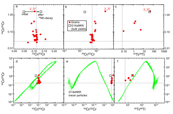
Figure 11: Comparison of isotopic ratios measured in pre-solar oxide grains (Dauphas et al., 2010; Qin et al., 2011; Nittler et al., 2018) compared to predictions of G14a simulation with NNK weak reaction rates. Open squares are bulk yields of G14aNKK, while green points (lower panels) are individual tracer particles. We note that the scales are different in the upper and lower panels. The dashed lines indicate solar ratios. Grain ${}^{50}\mathrm{Ti}$/${}^{48}\mathrm{Ti}$ ratios are calculated on the assumption that all measured signal at mass 50 is due to ${}^{50}\mathrm{Ti}$ (i.e., ${}^{50}\mathrm{Cr}$/${}^{52}\mathrm{Cr}$=0; Nittler et al., 2018).

Primitive chondritic meteorites preserve a record of the starting materials and earliest conditions of the formation of the solar system. Among their constituents are “pre-solar grains,” nm- to $\mu$-m sized mineral grains with extremely unusual isotopic compositions indicating that they originated in winds and explosions of ancient stars (see, e.g. Hoppe & Zinner, 2000) and were part of the protosolar molecular cloud. The vast majority of pre-solar grains, including many types of silicates, oxides, carbides, and graphite, are inferred to have formed in low-mass AGB stars or FeCCSNe. High-density SNe Ia such as those modelled by Woosley (1997) were suggested as the progenitors of a small number of $\lesssim$100-nm-diameter Cr-rich oxide grains from the Orgueil meteorite with large excesses in ${}^{54}\mathrm{Cr}$ relative to solar system materials (Dauphas et al., 2010; Qin et al., 2011). However, the grains in these studies were not fully spatially resolved on sample mounts and a FeCCSN origin could not be ruled out. Recently, Nittler et al. (2018) reported data for several additional such grains from Orgueil, acquired with substantially better spatial resolution. These measurements revealed a much broader range of ${}^{54}\mathrm{Cr}$/${}^{52}\mathrm{Cr}$ ratios than in previous studies, as well as resolved anomalies in ${}^{53}\mathrm{Cr}$ and/or at mass 50 in some grains. Nittler et al. (2018) showed that large excesses at mass 50 are most likely due to excess ${}^{50}\mathrm{Ti}$, which could not be resolved from ${}^{50}\mathrm{Cr}$ in these measurements. Nittler et al. (2018) further showed that the grains’ compositions were in reasonably good agreement with the predictions of Woosley (1997) for high-density SNe Ia and of Wanajo et al. (2013a) for cECSNe. It is thus useful to compare our tECSNe nucleosynthesis calculations with the measured pre-solar grain isotopic compositions.

The Cr- and Ti-isotopic data for the ${}^{54}\mathrm{Cr}$-rich pre-solar grains are compared with the bulk yields of the G14a simulation with the NKK04 weak reaction rates in Figures 11a-c. The simulation provides an almost-perfect match to the ${}^{54}\mathrm{Cr}$/${}^{52}\mathrm{Cr}$ ratio of the most extreme grain, 2-37. As seen before for the yields of high-density SNe Ia and cECSNe (Nittler et al., 2018), the predicted ${}^{50}\mathrm{Cr}$/${}^{52}\mathrm{Cr}$ ratio lies far below the grain data (Figure 11b), especially the five grains with ${}^{50}\mathrm{Cr}$/${}^{52}\mathrm{Cr}$$>$0.1, all of which also have apparent ${}^{50}\mathrm{Cr}$ enrichments (Figure 11b). Most likely, much of the measured signal at mass 50 in the grains is probably due to ${}^{50}\mathrm{Ti}$ rather than to ${}^{50}\mathrm{Cr}$. The inferred ${}^{50}\mathrm{Ti}$/${}^{48}\mathrm{Ti}$ ratios for these five grains, calculated on the assumption that all measured mass-50 signal is indeed ${}^{50}\mathrm{Ti}$, are shown in Figure 11c. Again, the predicted G14a bulk ejecta is in remarkable agreement with grain 2-37 (Figure 11c). The grains with more modest ${}^{54}\mathrm{Cr}$ enrichments have close-to-solar ${}^{50}\mathrm{Cr}$/${}^{52}\mathrm{Cr}$ ratios. Most likely the measured mass-50 signals for these grains are primarily due to ${}^{50}\mathrm{Cr}$, since if they were instead due to ${}^{50}\mathrm{Ti}$, the proximity of the data to the solar ${}^{50}\mathrm{Cr}$/${}^{52}\mathrm{Cr}$ ratio would require a highly improbable coincidence of Ti contents and ${}^{50}\mathrm{Ti}$/${}^{48}\mathrm{Ti}$ ratios. That said, the Cr isotopic data for these grains are far from the G14a predictions. This may reflect mixing of the supernova ejecta with more solar-like material, e.g., circumstellar material ejected prior to the explosion. Two predicted ${}^{53}\mathrm{Cr}$/${}^{52}\mathrm{Cr}$ ratios are shown in Figure 11a, one corresponding to directly after the explosion and one to after 0.3 Gyr, by which time all ${}^{53}\mathrm{Mn}$ ($t_{1/2}$=3.7 Myr) has fully decayed; the composition of 2-37 lies in between. If this grain formed in a tECSN as simulated by G14a bulk yields, this would thus require that some of the measured ${}^{53}\mathrm{Cr}$ was originally synthesized as ${}^{53}\mathrm{Mn}$. To preserve the highly anomalous isotopic signatures seen without dilution by circumstellar or interstellar matter, grain 2-37 most likely formed within a few years of the explosion, far shorter than the lifetime of ${}^{53}\mathrm{Mn}$. Therefore, if a significant fraction of the observed ${}^{53}\mathrm{Cr}$ was indeed due to ${}^{53}\mathrm{Mn}$ decay, Mn must have condensed into the grains at the time that they formed; the G14a yields would require that grain 2-37 had a few % stable ${}^{55}\mathrm{Mn}$. Indeed, spinel minerals (a likely form of the pre-solar ${}^{54}\mathrm{Cr}$-rich grains Dauphas et al., 2010) can accommodate Mn in their structure and future measurements of Mn in ${}^{54}\mathrm{Cr}$-rich grains could test this hypothesis. Alternatively, the discrepancy in ${}^{53}\mathrm{Cr}$ between the model and the data may indicate that the ejecta was not fully mixed before the grain condensed, as discussed further below.

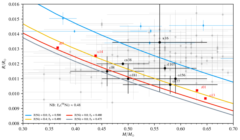
Figure 12: Theoretical white dwarf mass-radius relations for the surviving ONeFe bound remnants of the high-density ONe deflagration simulations by Jones et al. (2016b). The four curves are for different ONeFe white dwarfs with Fe-group mass fractions $X(\mathrm{Ni})$ represented by ⁵⁶Ni and ⁶⁴Ni mixed in a ratio to give the corresponding average $Y_{\mathrm{e}}$ for the white dwarf. The blue curve is for pure ONe white dwarfs. The grey points are the measurements from Bédard et al. (2017), the blue points are measurements from Joyce et al. (2018) which have vastly improved distance estimates from GAIA, and the black points are individual objects that have proposed as being either Fe white dwarfs or having Fe cores: Provencal et al. (1998, CD38-10980; G181-B58; G156-64), Catalán et al. (2008, C08; WD0433+270), Kepler et al. (2016, K16; SDSSJ124043.01), Bédard et al. (2017, J1107; SCR J1107-342). The red points are the bound remnants from the simulations by Jones et al. (2016b) and this work (see Table 2).

It is possible that the ejecta of a tECSN would not be fully mixed prior to condensation of dust grains. To explore the range of compositions that might be expected, the grain data are again compared to the G14a simulation in Figures 11d-f, only in this case the predicted compositions of $\sim$32,000 tracer particles are shown in addition to the bulk yields. These tracer particles contain essentially all of the ejected ${}^{54}\mathrm{Cr}$, and about 80% of the total ejected Cr. The remaining tracers contain either extremely small amounts of Cr or very ${}^{54}\mathrm{Cr}$-poor Cr (with variable ${}^{50}\mathrm{Cr}$) and are excluded from the plots for clarity. Figure 11d shows that the full range of ${}^{53}\mathrm{Cr}$/${}^{52}\mathrm{Cr}$ and ${}^{54}\mathrm{Cr}$/${}^{52}\mathrm{Cr}$ ratios observed in the grains could be explained by the model, if the ejecta were not fully mixed, obviating the need to incorporate radioactive ${}^{53}\mathrm{Mn}$ in the grains. The inability of this model to explain the grains’ measured ${}^{50}\mathrm{Cr}$/${}^{52}\mathrm{Cr}$ ratios is even clearer for the tracer particles than the bulk yields (Figure 11e). Again, the most extreme measured mass-50 excesses most likely indicate the presence of ${}^{50}\mathrm{Ti}$ enrichments (Figure 11f). In this case, the tracer particles are largely more ${}^{50}\mathrm{Ti}$-rich than the grain compositions, perhaps indicating a small amount of mixing with solar-like material.

In summary, the predicted Cr and Ti-isotopic compositions of the ejecta of a tECSN, as represented by the G14a simulation, are in remarkably good agreement with the most extreme reported ${}^{54}\mathrm{Cr}$-rich pre-solar grain and the grain data as a whole can be reasonably explained by the model when individual ejecta tracer particles are considered. As discussed by Nittler et al. (2018), an ECSN origin for the grains is attractive in that the lifetime of the parent star (of the order of 20 Myr) is comparable to the timescale of star-forming regions and it may be thus more reasonable to expect an association of dust from such an explosion with the forming solar system than from a SN Ia. An additional advantage of the present model is that, unlike the case of a cECSN (e. g., Wanajo et al., 2013a), a substantial amount of O is ejected by tECSN, making it more plausible for oxide grains to condense. The predicted O is essentially pure ${}^{16}{\mathrm{O}}$ and thus O-isotopic measurements of future ${}^{54}\mathrm{Cr}$-rich grains may provide additional constraints on their origin.

7 Bound ONeFe white dwarf remnants

In the simulations that do not collapse into neutron stars, only part of the ONe core becomes gravitationally unbound owing to energy release in thermonuclear burning, leaving behind a gravitationally bound remnant consisting of ¹⁶O, ²⁰Ne and some of the ashes of the deflagration (Nomoto & Kondo, 1991; Isern et al., 1991; Canal et al., 1992; Jones et al., 2016b). If such events do actually occur, and occur frequently enough, then they should be represented in the Galactic white dwarf population.

7.1 WD mass-radius relations for bound ONeFe remnants

We have constructed theoretical mass-radius relations for the bound ONeFe WD remnants left behind by tECSNe. There are now several known candidate WDs that we compare with our mass-radius relations and demonstrate could potentially be the gravitationally bound remnants of these explosions.

Using the equation of state by Potekhin & Chabrier (2010) we have constructed hundreds of spherically symmetric isothermal, uniform-composition white dwarf models in hydrostatic equilibrium using a Cash-Karp type Runge-Kutta integrator (Cash & Karp, 1990) starting from a given central density and integrating outwards to the surface, from which we have constructed theoretical white dwarf mass–radius relations for the bound remnants. The WDs are assumed to have no H or He layer at the surface. A range of compositions are possible outcomes from the hydrodynamic simulations, characterized by some fraction of Fe-group isotopes and an average $Y_{\mathrm{e}}$ (see Jones et al., 2016b, their Table 1). We have therefore chosen to use a two-parameter model for the white dwarf composition, where the ratio $X(^{16}\mathrm{O})/X(^{20}\mathrm{Ne})$ is held constant at $0.65/0.35=1.86$ (i.e. the same as the initial conditions before the deflagration) and the mass fraction of Ni and the $Y_{\mathrm{e}}$ are varied. We have assumed for simplicity that the Ni is made up from the two isotopes ⁵⁶Ni and ⁶⁴Ni, whose ratio is determined by $Y_{\mathrm{e}}$. More explicitly, given an “Fe-group” mass fraction $X_{\mathrm{Ni}}$ and an average $Y_{\mathrm{e}}$, the composition is given by

$$X_{56}=8(2Y_{\mathrm{e}}-1)+X_{\mathrm{Ni}},$$ (6)

$$X_{64}=X_{\mathrm{Ni}}-X_{56}=-8(2Y_{\mathrm{e}}-1),$$ (7)

$$X_{16}=0.65(1-X_{\mathrm{Ni}}),$$ (8)

$$X_{20}=1-X_{\mathrm{Ni}}-X_{16}.$$ (9)

We plot the resulting mass–radius curves for $(X_{\mathrm{Ni}},Y_{\mathrm{e}})=\{(0,0.5),(0.4,0.49),(0.8,0.48),(0.8,0.475)\}$ in Figure 12. The blue curve is for pure ONe white dwarfs. We have also plotted in Figure 12 the measurements from Bédard et al. (2017) (grey points) and some individual objects that have been proposed to be either Fe white dwarf or Fe-core white dwarf candidates: Provencal et al. (1998, CD38-10980; G181-B58; G156-64), Catalán et al. (2008, C08; WD0433+270), Kepler et al. (2016, K16; SDSSJ124043.01), Bédard et al. (2017, J1107; SCR J1107-342). Several of the individually-named (black points) candidates are reasonably fit with the cold ONeFe WD mass-radius relations. Only K16 appears to be more consistent with an ONe WD, although its error bars are quite large and all of our theoretical mass-radius curves the ONeFe WDs pass through the error bars for K16. The cloud of grey points from Bédard et al. (2017) contain several candidates that could be cold ONeFe WDs according to our theoretical mass-radius relations; some of the extreme WDs (in the lower-left portion of the figure) do not appear to be consistent with an ONeFe WD although again the error bars are quite large. We note at this point that observational tests of the WD mass-radius relationship are subject to uncertainties in the distance and surface gravity measurements. Previously, the distance estimates provided the largest source of the uncertainty, but with the launch of the GAIA mission the distance uncertainties have been considerably reduced and the spectroscopic measurements of H lines (from which the surface gravity can be derived) now pose the largest uncertainty (see, e.g. Joyce et al., 2018). Data from Joyce et al. (2018) using GAIA parallax distances are included as blue points in Figure 12 – note the substantially reduced radius error bars. All of the WDs reported by Joyce et al. appear to be more consistent with ONe or CO WDs (which would lie in the upper right of the figure) than ONeFe WDs.

Also plotted in Figure 12 are some of the models from Jones et al. (2016b, red squares). The relevant properties (i.e. remnant masses, mass of Fe-group elements and average electron fraction) from Table 1 of Jones et al. (2016b) are repeated in Table 2 for convenience. The bound ONeFe WD remnants do not match particularly well with any individual observed candidate, although they do populate a similar portion of the mass-radius plane. The simulations G13, G14, J01 and J07 shown in Figure 12 did not include Coulomb corrections in the EoS. Models including these corrections yielded significantly larger bound remnant masses (see Table 2) and would be outside the domain of this figure to the lower right. There are also some white dwarf candidates with such larger masses reported by Vennes et al. (2017) that may be good fits for those simulations.

Table 7: Decayed mass fractions of elements in the bound ONeFe remnant and the ejected material of the G14 simulation from Jones et al. (2016b). Decays were performed over $10^{16}$ s.

Element	Z	ejecta	bound remnant
H	1	1.05e-09	2.30e-10
He	2	6.25e-05	3.58e-05
Li	3	3.81e-16	1.41e-15
B	5	3.98e-15	3.78e-15
C	6	4.74e-08	4.91e-08
N	7	9.97e-08	1.29e-07
O	8	3.68e-01	4.58e-01
F	9	4.11e-12	5.78e-12
Ne	10	1.85e-01	2.29e-01
Na	11	2.68e-08	3.64e-08
Mg	12	2.98e-03	3.91e-03
Al	13	2.30e-06	3.12e-06
Si	14	2.34e-02	2.87e-02
P	15	3.13e-06	4.18e-06
S	16	1.45e-02	1.75e-02
Cl	17	3.17e-06	3.61e-06
Ar	18	3.31e-03	3.93e-03
K	19	8.74e-07	1.08e-06
Ca	20	5.38e-03	6.54e-03
Sc	21	2.08e-08	2.47e-08
Ti	22	4.20e-03	1.94e-03
V	23	2.09e-04	1.03e-04
Cr	24	1.57e-02	7.92e-03
Mn	25	7.09e-03	3.83e-03
Fe	26	3.08e-01	1.94e-01
Co	27	5.19e-04	2.65e-04
Ni	28	5.35e-02	3.03e-02
Cu	29	9.99e-05	6.05e-05
Zn	30	6.80e-03	6.82e-03
Ga	31	2.05e-05	2.64e-05
Ge	32	1.29e-04	7.89e-04
As	33	4.37e-06	7.89e-06
Se	34	4.80e-04	4.12e-03
Br	35	3.13e-05	1.85e-04
Kr	36	3.95e-04	2.28e-03
Rb	37	1.30e-05	2.48e-05
Sr	38	5.84e-08	3.92e-07
Y	39	2.39e-09	6.56e-09
Zr	40	8.60e-10	1.62e-09
Nb	41	9.70e-14	5.28e-13
Mo	42	8.43e-15	7.92e-14
Tc	43	1.26e-42	8.20e-43
Ru	44	4.29e-17	1.80e-17

There are other WD candidates identified by Gänsicke et al. (2010) and Raddi et al. (2018) worth mentioning here. Unfortunately, the data for the WDs identified by Gänsicke et al. (2010) are insufficient to derive the WD mass, however their large O/C ratios imply that they are, or were, ONe WDs as opposed to CO WDs.

The WD LP 40-365 studied by Raddi et al. (2018) is estimated to have a radius of 0.18$\pm 0.01\leavevmode\nobreak\ R_{\odot}$, and a mass of 0.37${}^{+0.29}_{-0.17}$ $M_{\sun}$, placing it outside of the domain of Figure 12. This means that the white dwarf has more than ten times the radius that we would expect it to have from our hydrostatic cold ($2\times 10^{4}$ K) WD models of the bound ONeFe remnant. For the radius of the WD to be this large, the star would need to be substantially hotter, say $\sim 10^{7}$ K.

7.2 Atmospheric composition of LP 40-365

Raddi et al. (2018) were able to spectroscopically derive compositional information for several elements in the atmosphere of LP 40-365, and they compared the composition to published yields from CCSN simulations, SN Ia simulations (DDTs) and SN Iax simulations (pure deflagrations with/without hybrid C/O/Ne progentiors). The detection of Mn in the atmosphere suggests that the composition originated in a single-degenerate SN Ia (Seitenzahl et al., 2013a), and the fact that a WD still exists suggests that the explosion failed to gravitationally unbind the entire star (Kromer et al., 2013).

Both of these characteristics ([Mn/Fe]$>0$ and a gravitationally bound remnant) are shared by our ONe deflagration simulations of tECSNe. In Table 7 we give the decayed mass fractions of elements in the bound remnant and in the ejecta of the G14 simulation. We plot the ratios of the decayed elemental composition to Fe compared to the solar ratios for the bound remnant and the ejecta of simulation G14 in Figure 13. The ratios for Ca, Ti, Cr, Fe and Ni in the G14 simulation appear to fit the data very well. The simulation produces a super-solar ratio for Mn of [Mn/Fe]$=0.44$, which is approximately half that measured in LP 40-365 ([Mn/Fe]$=0.82\pm 0.18$) by Raddi et al. and outside of the error bars, but not wildly inconsistent. Sc and V present much larger tensions with the measurements of higher-mass elements and stand out as being the only obviously problematic elements heavier than Ca. For the rest of the intermediate-mass elements the agreement between G14 and LP 40-365 is very poor, and even for Ne the simulation is 3 dex below the observational data. One of the caveats of our current nucleosynthesis simulations is the assumption that the initial composition is a mixture of pure ¹⁶O and ²⁰Ne. This means that there is no Na or Mg, etc from the prior C burning phases. There is also no signature of the metals that would have been present in the cloud that the star formed from. Lastly, ECSNe should be most prevalent from stars in binary systems (see Section 4) in which we expect a He shell and/or H envelope to surround the ONe core, which could further influence the atmospheric composition of the bound ONeFe remnant from a tECSN. Accounting for these shortcomings could help to alleviate some of the tensions that our tECSN simulations have with the atmospheric composition of LP 40-365, however it seems unlikely that the large discrepancies in the light- and intermediate-mass elements can be completely resolved in this way.

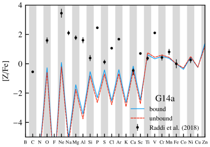
Figure 13: Elemental composition ratios ratio of the bound remnant and the unbound ejecta of the G14 simulation with respect to Fe and relative to the solar ratio. The black points are the spectroscopically determined composition of the atmosphere of the white dwarf LP 40-365 from Raddi et al. (2018). While the Ca, Ti, Cr, Fe and Ni abundances relative to Fe fit very well, the lighter elements are in distinct tension with the measurements.

8 Discussion of implications and concluding remarks

We have studied the nucleosynthesis in the ejecta and the bound ONeFe remnants of the thermonuclear ECSNe (tECSNe) from Jones et al. (2016b). The ejecta contains very large abundances of the neutron-rich isotopes ${}^{48}\mathrm{Ca}$, ${}^{50}\mathrm{Ti}$, ${}^{54}\mathrm{Cr}$ and ${}^{66}\mathrm{Zn}$ relative to solar. When weak reaction rates for fp- and fpg-shell nuclei (to the neutron-rich side of the pf shell) are included, the abundances of ${}^{48}\mathrm{Ca}$ and ${}^{66}\mathrm{Zn}$ are enhanced in the ejecta, the abundances of ${}^{50}\mathrm{Ti}$ and ${}^{54}\mathrm{Cr}$ are reduced and isotopes of the trans-iron elements Ge, Se and Kr are produced in greater abundance. The yields share many similarities with the core-collapse ECSN (cECSN) simulations by Wanajo et al. (2013a) and the high-density SNe Ia simulations by Woosley (1997). In the tECSNe scenario we present, ECSNe are the high-density SNe Ia.

The ejecta exhibits a high [Zn/Fe] ratio, which makes it an interesting candidate for explaining the high [Zn/Fe] in the early Milky Way, for which hypernovae are currently the most favourable scenario. The high [Ti/Fe] and [Mn/Fe] in the ejecta, if injected at early times into the Milky Way, could also help to alleviate the current tensions of GCE models with the observations of these two elements.

Owing to the low electron fractions achieved in portions of the ejecta, the $2.81\times 10^{-3}\leavevmode\nobreak\ M_{\sun}$ yield of ⁶⁰Fe is quite large – approximately ten or more times that of a FeCCSN. Perhaps more interestingly, owing to the different origin of ⁶⁰Fe in the tECSN scenario as compared with a FeCCSN, the molar ⁶⁰Fe/²⁶Al abundance ratio in the ejecta $Y(^{60}\mathrm{Fe})/Y(^{26}\mathrm{Al})=4.94\times 10^{4}$, which is $4-5$ orders of magnitude larger than what is expected from massive stars and FeCCSNe, which has interesting implications for interpreting the line ratio of 0.17 measured in the diffuse ISM by INTEGRAL/SPI. If the ²⁶Al from the progenitor envelope is included in the yield, the ratio in the tECSN is $Y(^{60}\mathrm{Fe})/Y(^{26}\mathrm{Al})\approx 130$, which is lower but still four orders of magnitude greater than the ISM value.

Using the solar abundance distribution and the FeCCSN yields from Nomoto et al. (2006), we place an upper limit on the occurrence of tECSNe to approximately $1-3\leavevmode\nobreak\ \%$ of the FeCCSN rate. This is in good agreement with the predictions from stellar evolution modelling and population synthesis simulations, which give $2-20\leavevmode\nobreak\ \%$ and $3-4\leavevmode\nobreak\ \%$, respectively. This is a somewhat surprising result and means that potentially all ECSNe being thermonuclear explosions does not apparently introduce an inconsistency between stellar evolution, binary population synthesis and galactic chemical evolution. If all ECSNe/AIC were tECSNe, this would mean that the Crab nebula is not the remnant of an ECSN (Davidson et al., 1982; Nomoto et al., 1982; Smith, 2013). Indeed, Woosley & Heger (2015) have shown that low-mass FeCCSNe could also be valid formation scenario for the Crab nebula and pulsar and Gessner & Janka (2018) demonstrate that the kick velocity of the Crab pulsar is more consistent with a low-mass FeCCSN than a cECSN. The outcome of the ONe deflagration is so sensitive to the prior evolution leading up to the ²⁰Ne electron capture phase and to the nuclear reaction rates themselves, amongst other things, that it is not impossible that both collapses and partial thermonuclear explosions could occur.

If accreting ONe WDs in ultra-close binaries undergoing stable mass transfer and retaining mass eventually undergo AIC but do not collapse into neutron stars (but are instead thermonuclear explosions), then they would no longer be candidates for forming low mass black holes (BHs, e.g. Belczynski & Taam, 2004). It is indeed currently the case that these low mass BHs have not been observed in binary systems, which is consistent with the scenario that AIC events do not produce NSs.

The isotopic ratios ${}^{54}\mathrm{Cr}$/${}^{52}\mathrm{Cr}$ and ${}^{50}\mathrm{Ti}$/${}^{48}\mathrm{Ti}$ (and ${}^{53}\mathrm{Cr}$/${}^{52}\mathrm{Cr}$ if the grains condense before mixing with the ISM) in a sub-set of meteoritic pre-solar oxide grains that have been identified as having extremely large ${}^{54}\mathrm{Cr}$ and ${}^{50}\mathrm{Ti}$ abundances are able to be very well reproduced by our tECSN simulations. The agreement is quite remarkable in fact. The close-to-solar ${}^{50}\mathrm{Cr}$/${}^{52}\mathrm{Cr}$ ratios measured in less anomalous (though still ${}^{54}\mathrm{Cr}$-enriched) grains, on the other hand, are much more difficult to match with the tECSN simulations and may require mixing of the ejecta with unprocessed pre-supernova material. tECSNe are very good candidates for explaining these types of oxide grains because there is a substantial amount of O in the ejecta, which is not the case for the yields of cECSNe.

The bound ONeFe WD remnants that tECSNe are expected to leave behind also look to be consistent with several observed candidate WDs. Theoretical mass-radius relation curves computed with typical remnant compositions pass through the error bars for several such objects. Unfortunately, for one particular object LP 40-365 where there is a spectroscopically-determined elemental composition for the WD’s atmosphere our WD remnants are far too small. This could be remedied if the remnants were hotter (about $10^{7}$ K), but even then we are unable to explain the entire composition in a satisfactory manner. For a sub-set of the elements though, including Ca, Ti, Cr, Mn, Fe and Ni, our model does match very well. Much more accurate parallax distances of WDs are available with the GAIA mission, making the spectroscopic determination of the surface gravities of WDs now the most uncertain aspect of constraining the observed WD mass-radius relation, which should help in either confirming or denying whether some or all ECSNe are tECSNe.

The rate predictions made in this paper using 3D hydrodynamics simulations and nucleosynthesis are fortunately not plagued by the difficult challenges of modelling the TP-SAGB phase of super-AGB stars or the convectively-bounded flames of low-mass FeCCSN progenitors, however they do have their own, sizeable, baggage attached. This includes the accuracy of the fp- and fpg-shell nuclear data, initial conditions for the modelling of the deflagration front and the precise ignition density of the deflagration. Many of these uncertainties are adequately discussed by Jones et al. (2016b) to which the interested reader is referred for further reading.