Bright Opportunities for Atmospheric Characterization of Small Planets: Masses and Radii of K2-3 b, c, d and GJ3470 b from Radial Velocity Measurements and Spitzer Transits

Abstract

We report improved masses, radii, and densities for four planets in two bright M-dwarf systems, K2-3 and GJ3470, derived from a combination of new radial velocity and transit observations. Supplementing K2 photometry with follow-up Spitzer transit observations refined the transit ephemerides of K2-3 b, c, and d by over a factor of 10. We analyze ground-based photometry from the Evryscope and Fairborn Observatory to determine the characteristic stellar activity timescales for our Gaussian Process fit, including the stellar rotation period and activity region decay timescale. The stellar rotation signals for both stars are evident in the radial velocity data and are included in our fit using a Gaussian process trained on the photometry. We find the masses of K2-3 b, K2-3 c and GJ3470 b to be 6.48${}^{+0.99}_{-0.93}$, 2.14${}^{+1.08}_{-1.04}$, and 12.58${}^{+1.31}_{-1.28}$ M_⊕ respectively. K2-3 d was not significantly detected and has a 3$\sigma$ upper limit of 2.80 M_⊕. These two systems are training cases for future TESS systems; due to the low planet densities ($\rho$ $<$ 3.7 g cm^-3) and bright host stars (K $<$ 9 mag), they are among the best candidates for transmission spectroscopy in order to characterize the atmospheric compositions of small planets.

1 Introduction

The field of exoplanets has shifted from detection to characterization due to technological improvements in instrumentation and large detection surveys such as NASA’s Kepler mission. One of the most surprising results from Kepler was the prevalence of planets between 1 and 4R_⊕, called super-Earths or sub-Neptunes , which are absent from our solar system (Howard et al., 2012; Dressing & Charbonneau, 2013, 2015; Fressin et al., 2013; Petigura et al., 2013). Planets of this size occur more frequently around M stars than G or F stars (Mulders et al. (2015) for orbital periods of $<$ 150 days).

Core-accretion models predict that an intermediate sized planet will become the core of a gas giant through runaway gas accretion. Therefore, these models are at odds with the prevalence of such intermediate mass planets (Mizuno, 1980; Bodenheimer & Lissauer, 2014). To avoid this problem, Lee et al. (2014) and Lee & Chiang (2016) proposed that super-Earths formed later than gas giants, without time to undergo runaway gas accretion. It is also debated whether there is sufficient material in the inner protoplanetary disk to form these planets (Weidenschilling, 1977; Hayashi, 1981). Pebble accretion and migration could address this problem and form closely packed multiplanet systems orbiting M dwarfs (Swift et al., 2013; Ormel et al., 2017).

Planet compositions provide a crucial link to their formation histories. The composition can be inferred either from the bulk density, which is derived from the planet’s mass and radius, or from atmospheric studies. Kepler transits and ground-based radial velocity (RV) follow-up discovered an increase in bulk density with decreasing size, suggesting a transition region at 1.5–2.0 R_⊕ between volatile-rich gas/ice planets and rocky planets (Weiss & Marcy, 2014; Rogers, 2015; Fulton et al., 2017; Van Eylen et al., 2017).

Due to the approaching launch of the James Webb Space Telescope (JWST) and selection for future European Space Agency (ESA) mission ARIEL, preparatory measurements of potential atmospheric characterization targets are important for identifying the best targets as well as for the interpretation of the spectra. Primarily, target ephemerides must be refined in order to reduce the transit timing uncertainty and therefore use space-based time most efficiently. Furthermore, precise mass measurements and surface gravity calculations are necessary as these parameters will affect the interpretation of the transmission spectra. Both atmospheric scale height and molecular absorption affect the depth of the planet’s spectroscopic features. Since atmospheric scale height is related to the surface gravity, a precise mass measurement is needed in order to correctly interpret the molecular absorption features in a spectrum (Batalha et al., 2017a).

The K2 mission has discovered many cool planets orbiting bright stars (Montet et al., 2015; Crossfield et al., 2016; Vanderburg et al., 2016; Dressing et al., 2017; Mayo et al., 2018), and TESS will find a large sample of even brighter systems around nearby stars (Ricker et al., 2014; Sullivan et al., 2015). These bright host stars can be more precisely followed up from ground-based telescopes and are amenable to transmission spectroscopy observations. This paper illustrates a follow-up program to prepare for potential JWST observations of two systems much like those that will be found by TESS.

In this paper we describe precise RV and photometry follow-up of two systems, K2-3 and GJ3470. Both of these systems have sub-Neptune-sized planets orbiting M-dwarf stars and are amenable to atmospheric transmission spectroscopy. In Section 2 we describe the two systems. In Section 3 we detail our Spitzer observations and analysis. In Section 4 we describe our RV analysis and related photometric follow-up, then present our RV results. In Section 5 we examine these planets in the context of other similar sub-Neptune systems and discuss atmospheric transmission spectroscopy considerations before concluding in Section 6.

2 Target Systems and Stellar Parameters

K2-3 (EPIC 201367065) is a bright (Ks = 8.6 mag), nearby (45 $\pm$ 3 pc) M0 dwarf star hosting three planets from 1.5 to 2 R_⊕ at orbital periods between 10 and 45 days (Crossfield et al., 2015a)(Table 1). These planets receive 1.5–10 times the flux incident on Earth; planet d orbits near the habitable zone.

Table 1: K2-3 Stellar Properties

Parameter	Value	Units	Source
Identifying Information
RA	11:29:20.388		(1)
DEC	-01:27:17.23		(1)
Photometric Properties
J	9.421 $\pm$ 0.027	mag	(2)
H	8.805 $\pm$ 0.044	mag	(2)
K	8.561 $\pm$ 0.023	mag	(2)
Kp	11.574	mag	(3)
Rotation Period	40 $\pm$ 2	days	(4)
Spectroscopic Properties
Barycentric RV	32.6 $\pm$ 1	km s-1	(1)
Distance	45 $\pm$ 3	pc	(1)
H$\alpha$	0.38 $\pm$ 0.06	Ang	(1)
Age	$\geq 1$	Gyr	(1)
Spectral Type	M0.0 $\pm$ 0.5 V		(1)
$[$Fe/H$]$	-0.32 $\pm$ 0.13		(1)
Temperature	3896 $\pm$ 189	K	(1)
Mass	0.601 $\pm$ 0.089	M⊙	(1)
Radius	0.561 $\pm$ 0.068	R⊙	(1)
Density	3.58 $\pm$ 0.61	$\rho_{\odot}$	(5)
Surface Gravity	4.734 $\pm$ 0.062	cgs	(5)

Note. — (1) Crossfield et al. (2015a), (2) Cutri et al. (2003), (3) Huber et al. (2016), (4) this work, (5) Almenara et al. (2015).

K2-3 b, c, and d were discovered in K2 photometry (Crossfield et al., 2015a). Since then, there have been multiple RV and transit follow-up measurements. Almenara et al. (2015) collected 66 HARPS spectra and determined the masses of planet b, c, and d to be $8.4\pm 2.1$, $2.1^{+2.1}_{-1.3}$, and $11.1\pm 3.5$ M_⊕, respectively. Almenara et al. (2015) caution that the RV semi-amplitudes of planets c and d are likely affected by stellar activity. Dai et al. (2016) collected 31 spectra with the Planet Finder Spectrograph (PFS) on Magellan and modeled the RV data with Almenara’s HARPS data. The combined datasets constrained the masses of planets b, c, and d to be $7.7\pm 2.0$, $<12.6$, and $11.3^{+5.9}_{-5.8}$ M_⊕, respectively. Damasso et al. (2018) performed an RV analysis on a total of 132 HARPS spectra and 197 HARPS-N spectra, including the Almenara sample. This HARPS analysis found the mass of planet b and c to be 6.6 $\pm$ 1.1 and 3.1${}^{+1.3}_{-1.2}$ M_⊕, respectively. The mass of planet d is estimated as 2.7${}^{+1.2}_{-0.8}$ from a suite of injection-recovery tests. Beichman et al. (2016a) refined the ephemeris and radii of the three planets with seven follow-up Spitzer transits and Fukui et al. (2016) observed a ground-based transit of K2-3 d to further refine its ephemeris.

GJ3470 is also a bright ($K$ = 8.0 mag), nearby (29.9${}^{+3.7}_{-3.4}$ pc) M1.5 dwarf hosting one Neptune-sized planet in a 3.33 day orbit (Cutri et al., 2003; Bonfils et al., 2012)(Table 2). GJ3470 b was discovered in a HARPS RV campaign that searched for short-period planets orbiting M dwarfs and was subsequently observed in transit. GJ3470 b has an equilibrium temperature near 700 K and a radius of 3.9 R_⊕. Its mass has been measured previously to be 13.73$\pm$1.61, 14.0$\pm$1.8, and 13.9${}^{+1.5}_{-1.4}$ M_⊕ by Bonfils et al. (2012), Demory et al. (2013), and Biddle et al. (2014) respectively. Its low density supports a substantial atmosphere covering the planet (Biddle et al., 2014). Seven previous studies have investigated its atmospheric composition. Fukui et al. (2013) found variations in the transit depths in the $J$, $I$, and 4.5 $\mu$m bands that suggest that the atmospheric opacity varies with wavelength due to the absorption or scattering of stellar light by atmospheric molecules. Nascimbeni et al. (2013) detected a transit depth difference between the ultraviolet and optical wavelengths also indicating a Rayleigh-scattering slope, confirmed by Biddle et al. (2014); Chen et al. (2017) and Dragomir et al. (2015). Crossfield et al. (2013) found a flat transmission spectrum in the $K$-band suggesting a hazy, methane-poor, or high-metallicity atmosphere. Finally, Bourrier et al. (2018) find the planet is surrounded by a large exosphere of neutral hydrogen from Hubble Lyman alpha measurements.

Table 2: GJ3470 Stellar and Planet b Transit Properties

Parameter	Value	Units	Source
Photometric Properties
Spectral type	M1.5		(1)
$V$	12.3	mag	(2)
$K$	7.989 $\pm$ 0.023	mag	(3)
$J$	8.794 $\pm$ 0.019	mag	(3)
$H$	8.206 $\pm$ 0.023	mag	(3)
Rotation Period	21.54 $\pm$ 0.49	days	(5)
Spectroscopic Properties
Luminosity	0.029 0.002	L⊙	(2)
Mass	0.51 $\pm$ 0.06	M⊙	(4)
Radius	0.48 $\pm$ 0.04	R⊙	(4)
Distance	30.7${}^{+2.1}_{-1.7}$	pc	(6)
Age	0.3–3	Gyr	(2)
Temperature	3652 $\pm$ 50	K	(4)
Surface Gravity	4.658 $\pm$ 0.035	cgs	(6)
$[$Fe/H$]$	+0.20 $\pm$ 0.10		(6)
Transit Properties
T0 ($-2450000$)	6677.727712 $\pm$ 0.00022	BJD	(7)
T14	0.07992${}^{+0.00100}_{-0.00099}$	days	(7)
P	3.3366413$\pm$0.0000060	days	(7)
Rp	3.88 $\pm$ 0.32	R⊕	(4)
a/R∗	12.92${}^{+0.72}_{-0.65}$		(7)
Teq	615 $\pm$ 16	K	(2)

Note. — (1) Reid et al. (1997), (2) Bonfils et al. (2012), (3) Cutri et al. (2003), (4) Biddle et al. (2014), (5) this work, (6) Demory et al. (2013), (7) Dragomir et al. (2015).

3 K2-3 Spitzer Observations

We observed six transits of K2-3 b, two transits of K2-3 c, and two transits of K2-3 d using Channel 2 (4.5 $\mu$m) of the Infrared Array Camera (IRAC) on the Spitzer Space Telescope to refine the transit parameters of these three planets (GO 11026, PI: Werner; GO 12081, PI: Benneke). K2-3 was observed in staring mode and placed on the “sweet spot” pixel to keep the star in one location during the observations and minimize the effect of gain variations. To minimize data volume and overhead from readout time, the subarray mode was used with an exposure time of 2 seconds per frame. This produced between 11392 and 26368 individual frames per observation. Total observation durations were between 6.5 and 15 hours to include adequate out-of-transit baseline and were typically centered near the predicted mid-transit time from the K2 ephemeris.

In the following subsection, we describe two different analyses performed on these Spitzer data. The first analysis performs an individual fit to each Spitzer transit separately to check for consistency of the parameters between individual transit events whereas the second analysis performs a combined fit to the Spitzer data to derive global parameters.

3.1 Spitzer Transit Analysis

We extract the Spitzer light curves following the approach taken by Knutson et al. (2012) and Beichman et al. (2016b), using a circular aperture 2.4 pixels in radius centered on the host star. We used the Python package photutils (Bradley et al., 2016) for centroiding and aperture photometry. We use a modified version of the pixel-level decorrelation (PLD, Deming et al. (2015)) adapted from Benneke et al. (2017) to simultaneously model the Spitzer systematics (intra-pixel sensitivity variations) and the exoplanet system parameters. The instrument sensitivity is modeled by equation 1 in Benneke et al. (2017), and we use the Python package batman (Kreidberg, 2015) to generate the transit models. For parameter estimation we use the Python package emcee (Foreman-Mackey et al., 2013), an implementation of the affine-invariant Markov chain Monte Carlo (MCMC) ensemble sampler (Goodman & Weare, 2010). We find that using a $3\times 3$ pixel grid sufficiently captures the information content corresponding to the motion of the point-spread function (PSF) on the detector (which is typically $\lesssim$ a few tenths of a pixel). In comparisons between various methods used to correct Spitzer systematics (Ingalls et al., 2016), PLD was among the top performers, displaying both high precision and repeatability. For more details about this type of IRAC photometry analysis, see Livingston et al. (2019) and K. Hardegree-Ullman (2019, in preparation).

We first analyzed the Spitzer transits one at a time to check for consistency of parameters between independent transit events. For the individual transit models, we fit for the scaled planet radius $R_{p}/R_{\star}$, the mid-transit time $T_{0}$, the scaled semi-major axis $a/R_{\star}$, and the orbital inclination angle $i$. The quadratic limb-darkening coefficients for the 4.5$\mu$m Spitzer bandpass were found by interpolating the values from Claret et al. (2012a). We held the orbital periods constant at the values found by Beichman et al. (2016a), and fixed eccentricity and longitude of periastron to 0, but note that these parameters have a negligible effect on the overall shape of the transit model. Gaussian priors were imposed on the transit system parameters based on our previous knowledge of the system from Crossfield et al. (2015b). We also found global system parameters by combining the posterior distributions from each individual result for each planet and finding the 16th, 50th, and 84th percentiles of the combined distribution. One example transit is shown in Figure 1.

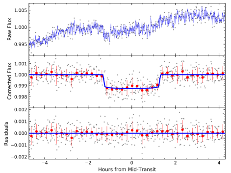
Figure 1: Example fit to one transit of K2-3 b. Top: raw Spitzer data (black points) including the fit to the systematics (blue line). middle: Transit of K2-3 b including raw data (grey points), binned data (red points), and transit model (blue line). Bottom: residuals from the model.

We then perform our global fit to the 10 Spitzer transit datasets of the three planets in this system by constructing a joint model comprising a set of shared transit parameters and a set of systematic parameters corresponding to each individual transit observation. We adopt a global quadratic limb-darkening law and set Gaussian priors on the parameters $u_{1}$ and $u_{2}$ by interpolating the table of Claret et al. (2012b), where the widths are determined by a Monte Carlo simulation. To restrict exploration of limb-darkening parameter space to only physical scenarios, we utilize the triangular sampling method of Kipping (2013); thus, we actually sample in $q_{1}$/$q_{2}$ space. For each of the three planets in the system, we use a unique set of transit parameters: the period $P$, time of mid-transit $T_{0}$, planet-star radius ratio $R_{P}/R_{\star}$, scaled semi-major axis $a/R_{\star}$, and impact parameter $b$. The rest of the parameters in the model correspond to the PLD coefficients for each individual dataset. Besides the Gaussian priors on the limb-darkening parameters, we also impose Gaussian priors on $T_{0}$, $P$, and the mean stellar density of the host star, based on the values reported in Crossfield et al. (2015b). See Figure 2 for the transit fits for K2-3 b, c, and d obtained from our global Spitzer analysis.

All of our transit parameters are shown in Table 3 along with the parameters derived from only the K2 transits for comparison (Crossfield et al., 2015a). We combined the parameters from the individual fits by adding their posteriors in order to compare the individual fits with the global analysis. The parameters from these two analyses are all within 1$\sigma$. We adopt the parameters from the simultaneous transit analysis for our RV analysis.

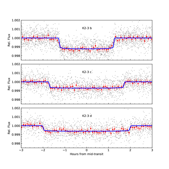
Figure 2: Transit fits to K2-3 b, c, and d displaying all of our Spitzer data for each planet. Individual Spitzer datapoints (grey), binned points (red), and planet fits from our simultaneous analysis (blue) for each K2-3 planet are shown.

Table 3: K2-3 Spitzer Transit Fit Parameters

Planet	P [days]	Mid-Transit [BJD]	$R_{p}/R_{\star}$ [%]	$R_{p}/R_{\oplus}$	$a/R_{\star}$	$i$ [∘]	$b$	Source
b	–	$2457094.94680^{+0.00080}_{-0.00068}$	$3.494^{+0.087}_{-0.087}$	$2.134^{+0.272}_{-0.260}$	$29.44^{+3.89}_{-3.91}$	$89.50^{+0.35}_{-0.43}$	$0.26^{+0.21}_{-0.17}$	IRAC2 Transit 1
b	–	$2457105.00241^{+0.00068}_{-0.00062}$	$3.864^{+0.094}_{-0.095}$	$2.366^{+0.298}_{-0.300}$	$29.478^{+3.93}_{-3.88}$	$89.56^{+0.30}_{-0.39}$	$0.23^{+0.19}_{-0.16}$	IRAC2 Transit 2
b	–	$2457275.92778^{+0.00149}_{-0.00121}$	$3.355^{+0.090}_{-0.090}$	$2.053^{+0.259}_{-0.258}$	$29.54^{+3.91}_{-3.99}$	$89.31^{+0.45}_{-0.50}$	$0.35^{+0.25}_{-0.23}$	IRAC2 Transit 3
b	–	$2457466.97119^{+0.00114}_{-0.00086}$	$3.360^{+0.084}_{-0.085}$	$2.057^{+0.253}_{-0.260}$	$29.43^{+3.89}_{-3.95}$	$89.46^{+0.37}_{-0.46}$	$0.27^{+0.23}_{-0.18}$	IRAC2 Transit 4
b	–	$2457497.13286^{+0.00107}_{-0.00111}$	$3.659^{+0.088}_{-0.088}$	$2.237^{+0.286}_{-0.271}$	$29.52^{+4.02}_{-4.00}$	$89.42^{+0.40}_{-0.49}$	$0.30^{+0.24}_{-0.20}$	IRAC2 Transit 5
b	–	$2457627.84302^{+0.00090}_{-0.00232}$	$3.572^{+0.090}_{-0.091}$	$2.192^{+0.267}_{-0.266}$	$29.46^{+3.89}_{-3.92}$	$89.52^{+0.33}_{-0.44}$	$0.25^{+0.21}_{-0.17}$	IRAC2 Transit 6
b	$10.054638\pm 0.000016$	–	$3.532^{+0.243}_{-0.185}$	$2.165^{+0.297}_{-0.284}$	$29.43^{+3.93}_{-3.91}$	$89.47^{+0.37}_{-0.46}$	$0.27^{+0.22}_{-0.19}$	Individual Combined
b	$10.054626^{+0.000009}_{-0.000010}$	$2456813.41843^{+0.00039}_{-0.00038}$	$3.44^{+0.04}_{-0.04}$	$2.103^{+0.257}_{-0.256}$	$30.02^{+0.25}_{-0.31}$	$89.588^{+0.116}_{-0.100}$	$0.22^{+0.05}_{-0.06}$	Simultaneous Fit
b	10.05403${}^{+0.00026}_{-0.00025}$	2456813$\pm$0.0011	3.483${}^{+0.123}_{-0.070}$	2.14${}^{+0.27}_{-0.26}$	29.2${}^{+1.8}_{-3.6}$	89.28${}^{+0.46}_{-0.60}$	0.37${}^{+0.22}_{-0.23}$	Crossfield et al. (2015a)
c	–	$2457108.03664^{+0.00172}_{-0.00187}$	$2.549^{+0.080}_{-0.081}$	$1.557^{+0.197}_{-0.190}$	$53.62^{+7.12}_{-7.13}$	$89.73^{+0.21}_{-0.27}$	$0.29^{+0.24}_{-0.19}$	IRAC2 Transit 1
c	–	$2457280.56131^{+0.00215}_{-0.00224}$	$2.554^{+0.080}_{-0.081}$	$1.559^{+0.198}_{-0.195}$	$53.28^{+7.19}_{-7.23}$	$89.69^{+0.21}_{-0.27}$	$0.28^{+0.24}_{-0.20}$	IRAC2 Transit 2
c	–	$2457477.73145^{+0.00254}_{-0.00253}$	$2.670^{+0.081}_{-0.081}$	$1.635^{+0.204}_{-0.200}$	$53.30^{+7.15}_{-7.07}$	$89.72^{+0.19}_{-0.26}$	$0.26^{+0.24}_{-0.18}$	IRAC2 Transit 3
c	–	$2457625.61918^{+0.00171}_{-0.00199}$	$2.726^{+0.077}_{-0.081}$	$1.668^{+0.211}_{-0.207}$	$53.49^{+7.10}_{-7.03}$	$89.73^{+0.19}_{-0.25}$	$0.26^{+0.22}_{-0.19}$	IRAC2 Transit 4
c	–	$2457650.26528^{+0.00191}_{-0.00129}$	$2.743^{+0.079}_{-0.079}$	$1.680^{+0.209}_{-0.207}$	$53.67^{+7.00}_{-7.01}$	$89.72^{+0.19}_{-0.24}$	$0.26^{+0.22}_{-0.18}$	IRAC2 Transit 5
c	$24.646569\pm 0.000047$	–	$2.653^{+0.116}_{-0.128}$	$1.618^{+0.212}_{-0.207}$	$53.47^{+7.10}_{-7.15}$	$89.71^{+0.20}_{-0.26}$	$0.27^{+0.23}_{-0.19}$	Individual Combined
c	$24.646582^{+0.000039}_{-0.000039}$	$2456812.28013^{+0.00090}_{-0.00095}$	$2.59^{+0.06}_{-0.06}$	$1.584^{+0.197}_{-0.195}$	$54.57^{+0.46}_{-0.56}$	$89.905^{+0.066}_{-0.088}$	$0.09^{+0.08}_{-0.06}$	Simultaneous Fit
c	24.6454$\pm$0.0013	2456812${}^{+0.00026}_{-0.00025}$	2.786${}^{+0.143}_{-0.083}$	1.72${}^{+0.23}_{-0.22}$	51.8${}^{+4.1}_{-9.1}$	89.55${}^{+0.29}_{-0.44}$	0.41${}^{+0.26}_{-0.25}$	Crossfield et al. (2015a)
d	–	$2457093.56831^{+0.00517}_{-0.00325}$	$2.479^{+0.089}_{-0.089}$	$1.521^{+0.191}_{-0.190}$	$79.09^{+10.55}_{-10.73}$	$89.81^{+0.13}_{-0.17}$	$0.27^{+0.23}_{-0.19}$	IRAC2 Transit 1
d	–	$2457271.79827^{+0.00477}_{-0.00359}$	$2.490^{+0.088}_{-0.089}$	$1.521^{+0.194}_{-0.191}$	$79.74^{+10.63}_{-10.82}$	$89.81^{+0.13}_{-0.17}$	$0.27^{+0.23}_{-0.19}$	IRAC2 Transit 2
d	–	$2457494.57861^{+0.00405}_{-0.00296}$	$2.454^{+0.082}_{-0.083}$	$1.503^{+0.184}_{-0.191}$	$79.51^{+10.55}_{-10.67}$	$89.79^{+0.14}_{-0.17}$	$0.30^{+0.22}_{-0.20}$	IRAC2 Transit 3
d	–	$2457628.23815^{+0.00891}_{-0.00200}$	$2.449^{+0.081}_{-0.082}$	$1.500^{+0.189}_{-0.185}$	$79.69^{+10.78}_{-10.63}$	$89.80^{+0.14}_{-0.17}$	$0.29^{+0.24}_{-0.20}$	IRAC2 Transit 4
d	$44.556913\pm 0.000182$	–	$2.468^{+0.086}_{-0.087}$	$1.511^{+0.191}_{-0.193}$	$79.35^{+10.71}_{-10.53}$	$89.80^{+0.14}_{-0.17}$	$0.28^{+0.23}_{-0.19}$	Individual Combined
d	$44.556456^{+0.000097}_{-0.000087}$	$2456826.22347^{+0.00053}_{-0.00052}$	$2.44^{+0.08}_{-0.08}$	$1.492^{+0.189}_{-0.186}$	$80.98^{+0.68}_{-0.84}$	$89.788^{+0.033}_{-0.029}$	$0.30^{+0.04}_{-0.05}$	Simultaneous Fit
d	44.5631${}^{+0.0063}_{-0.0043}$	2456826${}^{+0.00037}_{-0.00043}$	2.48${}^{+0.14}_{-0.10}$	1.52${}^{+0.21}_{-0.20}$	78.7${}^{+6.7}_{-13}$	89.68${}^{+0.21}_{-0.26}$	0.45${}^{+0.23}_{-0.28}$	Crossfield et al. (2015a)

3.2 Spitzer Ephemeris Improvement

These Spitzer data reduce the uncertainty on the transit times and periods of the K2-3 planets. Refining the ephemerides is particularly important in order to efficiently subdivide time on large telescopes and space-based telescopes.  Figure 3 shows the uncertainty of the transit time of each planet propagated forwards to 2022, shortly after the launch of JWST. This refinement is crucial to accurately schedule transit observations with future space-based atmospheric missions. For example, if one wanted to observe K2-3 d in the JWST era, the K2 3$\sigma$ uncertainty of the transit mid-point is over 25 hours; this would waste considerable telescope time and will only increase as the time baseline lengthens. Beichman et al. (2016a) refined its ephemeris with Spitzer measurements two years ago. Our measurements further refine the orbital period uncertainty by a over factor of twenty from the original K2 data and to one-third of that from Beichman et al. (2016a). From our Spitzer analysis, the 3$\sigma$ uncertainty in the transit mid-point of K2-3 d in 2022 has improved to only 30 minutes.

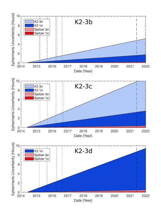
Figure 3: Transit time uncertainty for the K2-3 system in the JWST era. The blue region illustrates the 3$\sigma$ uncertainty (light blue) and 1$\sigma$ uncertainty (dark blue) on the transit times from the K2-derived ephemerides reported by Crossfield et al. (2015a). Equivalently, the red region illustrates the 1$\sigma$ and 3$\sigma$ uncertainty on the transit times from our Spitzer-derived ephemerides. The vertical dotted lines illustrate the times of the Spitzer observations. The vertical dashed line shows the scheduled JWST launch in March 2021. The Spitzer transits decrease the uncertainty on the transit times by over a factor of 10.

4 Radial Velocity Analysis

4.1 RV Observations

We obtained RV measurements of K2-3 and GJ3470 using the High Resolution Echelle Spectrometer (HIRES)(Vogt et al., 1994) on the Keck I Telescope. We collected 74 measurements of K2-3 from 2015 Feb 4 to 2017 Apr 11 and 56 measurements of GJ3470 from 2012 Sep 25 to 2017 Mar 15. These spectra were taken with an iodine cell and the C2 decker; a template spectrum was also taken in order to calibrate the wavelength and estimate the RV uncertainty. On average, measurements of K2-3 were collected with an exposure time of 1600s in order to reach a signal-to-noise ratio (S/N) of 87/pixel (80k counts on the HIRES exposure meter). Measurements of GJ3470 were collected with an exposure time of 1200s in order to reach a S/R of 60/pixel (40k counts). The observations and data reduction followed the California Planet Search method described in Howard et al. (2010). RV data for K2-3 and GJ3470 are shown in Table 4 and Table 5.

Table 4: K2-3 HIRES Relative RV Measurements

BJDTDB	RV (m/s)	Unc. (m/s)	$S_{\mathrm{HK}}$ $\pm$ 0.005
2457057.93921	0.366715	2.333335	0.9000
2457058.03821	-0.957106	1.734197	0.7805
2457058.05976	-3.153888	1.63551	0.7963
2457058.08085	-7.341192	1.583017	0.7784
2457058.92564	11.883496	1.898559	0.7086
2457058.95076	10.980076	2.34516	0.6743
2457058.97218	3.558983	2.28085	0.7210
2457059.08507	2.8289	1.947861	0.6640
2457059.10630	0.20892	1.917224	0.5664
2457059.13391	-1.2014	1.994416	0.5140
2457061.99505	0.377411	1.736609	0.7832
2457062.00959	3.934113	1.810443	0.8032
2457062.02387	4.739629	1.640702	0.8091
2457062.09685	-3.780676	1.574131	0.7972
2457062.11334	2.534422	1.596577	0.8000
2457062.13098	4.418034	1.67832	0.7943
2457150.95144	-8.490637	1.916942	0.7797
2457150.96587	-7.028363	1.936422	0.7828
2457179.79623	-8.162854	1.559401	0.7842
2457179.81064	-8.641193	1.509294	0.7974
2457179.82504	-10.420957	1.724975	0.7913
2457200.80146	-1.273851	1.799606	0.8192
2457200.81577	-2.722842	1.907786	0.7689
2457201.83038	-4.710788	2.031547	0.7397
2457208.77055	-6.80142	1.712294	0.7549
2457210.79928	-4.84792	2.040615	0.7334
2457213.81025	7.015119	1.824659	0.5133
2457216.77797	-8.124406	2.05162	0.6954
2457353.10152	4.475981	1.543244	0.7053
2457353.12056	0.028874	1.546589	0.7198
2457353.13925	-0.068528	1.601731	0.7463
2457354.10453	-0.48829	1.809439	0.7089
2457355.10054	1.319467	1.438562	0.7483
2457355.12162	-1.344597	1.361441	0.7516
2457355.14113	-1.368156	1.456596	0.7424
2457356.14169	-1.975064	1.440952	0.7642
2457379.16194	-4.437901	2.241596	0.6464
2457380.12667	-5.164231	1.315844	0.7863
2457402.09882	1.894179	1.464712	0.7416
2457412.01971	-5.863205	1.562807	0.7138
2457412.97043	-4.887563	1.686561	0.7082
2457440.00883	-0.910402	1.606493	0.8340
2457555.80733	1.681344	1.661285	0.8243
2457556.77194	-2.244875	2.209068	0.7812
2457561.77900	-7.481403	1.4887	0.7161
2457562.79062	-4.631916	1.580454	0.8505
2457568.76731	-10.052094	1.606564	0.7981
2457569.76509	-8.724515	1.558577	0.7550
2457582.75548	-3.797623	1.436803	0.6825
2457583.75403	-3.464112	1.364596	0.6969
2457584.75297	-1.794929	1.603735	0.7044
2457585.75810	-2.151584	1.60559	0.7309
2457586.75440	-3.55797	1.564322	0.3217
2457587.75599	-1.494904	1.358847	0.6771
2457595.74801	10.033845	2.654412	0.3791
2457598.74824	0.027648	2.425191	0.7842
2457704.13227	-0.506104	1.454338	0.6111
2457712.13329	-2.620005	1.708553	0.7164
2457713.13868	-2.609817	1.463878	0.7393
2457748.04174	6.208275	1.448043	0.6792
2457760.06409	-3.215456	1.623777	0.7917
2457764.05803	3.894852	2.171037	0.5624
2457764.07086	-7.417492	1.509814	0.7471
2457766.11836	1.378119	1.697936	0.6227
2457775.02567	-6.355654	1.394235	0.6265
2457776.02209	-6.467462	1.565302	0.6076
2457789.02271	-1.747466	1.475222	0.7479
2457790.06443	-1.473748	1.444261	0.7361
2457790.97319	-5.278218	1.465153	0.6644
2457793.02703	3.394093	1.45068	0.7481
2457794.05774	0.960206	1.40496	0.7684
2457807.14530	-5.723126	1.714786	0.6560
2457830.03452	0.125619	1.574956	0.7394
2457854.95873	-5.315930	1.674391	0.6144

Table 5: GJ3470 Relative RV Measurements

BJDTDB	RV (m/s)	Unc. (m/s)	$S_{\mathrm{HK}}$	Instrument
2456196.12523	7.288214	1.593834	.846	HIRES
2456203.092443	8.423508	1.834917	.905	HIRES
2456290.104424	6.622361	1.963188	.94	HIRES
2456325.977586	2.104225	1.866118	1.01	HIRES
2456326.975188	.832374	1.758792	.942	HIRES
2456327.88963	-7.895415	1.692606	.826	HIRES
2456343.870814	.923284	2.314857	1.33	HIRES
2456588.081082	-.35254	1.870567	1.13	HIRES
2456589.077408	.063746	1.937277	1.15	HIRES
2456614.065159	4.259696	1.6414	.94	HIRES
2456638.025333	.966082	1.984093	1.003	HIRES
2456639.072967	3.538801	2.074385	1.05	HIRES
2456674.864834	.191914	2.54771	.5569	HIRES
2456913.131531	9.193756	1.955105	1.011	HIRES
2457057.815422	10.436685	2.241942	.5531	HIRES
2457058.750372	-5.2962	2.076247	.7862	HIRES
2457058.873714	-8.422584	1.941071	.85	HIRES
2457060.982769	.678555	2.075819	.9992	HIRES
2457061.033057	6.206761	2.073267	1.228	HIRES
2457061.812464	-7.524646	1.785195	1.068	HIRES
2457061.94901	-6.276048	1.787998	.8942	HIRES
2457291.139283	5.543131	1.439182	.7674	HIRES
2457294.128406	7.733903	1.867845	1.421	HIRES
2457295.102025	3.158103	1.820473	.9017	HIRES
2457297.077797	11.011115	1.988343	1.009	HIRES
2457327.13922	1.997108	1.644166	.2899	HIRES
2457353.078119	-7.943347	2.093493	.9405	HIRES
2457353.944139	4.361439	1.818723	1.234	HIRES
2457355.060478	-7.495449	1.706797	1.067	HIRES
2457356.064562	-8.723251	2.051534	1.004	HIRES
2457379.916768	-4.3828	1.77893	1.109	HIRES
2457413.787232	9.647246	2.030947	.8166	HIRES
2457414.914383	7.061204	1.988887	1.079	HIRES
2457422.800915	-15.693013	1.906881	.9322	HIRES
2457653.107039	-4.250508	1.991533	.2492	HIRES
2457654.104405	3.586683	1.673021	.9448	HIRES
2457669.122191	-14.811282	1.578996	1.148	HIRES
2457672.13511	-11.112049	1.828574	1.234	HIRES
2457673.081487	-13.188282	1.909879	.9718	HIRES
2457679.036588	-5.932064	2.144353	1.578	HIRES
2457698.092274	-1.030799	1.614768	.961	HIRES
2457704.037282	2.59695	1.831448	.9315	HIRES
2457715.110143	-2.959431	1.638235	.8807	HIRES
2457716.043219	-9.729558	1.768124	1.031	HIRES
2457717.029436	-2.234329	1.714418	.9169	HIRES
2457746.949718	-.646912	1.913229	1.259	HIRES
2457747.976742	11.546778	1.926047	1.006	HIRES
2457760.011365	-9.438351	1.810585	1.073	HIRES
2457761.933534	-3.068847	2.321973	.8624	HIRES
2457763.825522	-3.939269	1.78412	2.341	HIRES
2457774.850285	13.127662	1.996166	1.025	HIRES
2457775.809841	2.277267	1.93025	1.117	HIRES
2457787.841488	6.761939	1.818927	.9395	HIRES
2457789.764085	-11.138971	1.723854	1.033	HIRES
2457790.753742	6.147943	1.950918	1.051	HIRES
2457828.957103	-.62745	2.03147	1.235	HIRES
2455987.609282	26499.6	5.53	–	HARPS
2455988.600211	26509.13	3.66	–	HARPS
2455989.61836	26520.36	4.12	–	HARPS
2455998.576091	26491.47	4.28	–	HARPS
2455999.591694	26512.37	4.39	–	HARPS
2456000.582575	26493.87	3.92	–	HARPS
2456004.556958	26499.35	4.41	–	HARPS
2456006.601714	26505.11	3.59	–	HARPS
2456009.541376	26508.57	3.51	–	HARPS
2456010.556922	26496.39	3.12	–	HARPS
2456020.540282	26500.09	3.76	–	HARPS
2456021.516266	26484.51	4.64	–	HARPS
2456022.539385	26508.62	4.53	–	HARPS
2456024.514473	26486.41	3.93	–	HARPS
2456026.493726	26505.56	4.99	–	HARPS
2456030.52744	26507.06	6.71	–	HARPS
2456052.469466	26508.64	3.61	–	HARPS
2456053.450485	26502.98	3.56	–	HARPS
2456054.474948	26488.64	7.07	–	HARPS
2456056.456245	26502.6	3.37	–	HARPS
2456058.446999	26494.33	3.22	–	HARPS
2456060.445313	26495.35	3.04	–	HARPS
2456062.441639	26502.2	3.89	–	HARPS
2456253.864979	26500.27	3.54	–	HARPS
2456254.863141	26490.16	3.79	–	HARPS
2456256.842426	26503.37	4.44	–	HARPS
2456258.844023	26497.3	4.5	–	HARPS
2456259.821681	26512.3	6.12	–	HARPS
2456285.804381	26504.38	4.06	–	HARPS
2456286.769862	26505.39	3.95	–	HARPS
2456287.774812	26494.21	5.19	–	HARPS
2456321.69114	26492.16	4.62	–	HARPS
2456360.575823	26506.15	4.55	–	HARPS
2456367.577169	26496.9	3.81	–	HARPS
2456374.535139	26486.66	3.63	–	HARPS
2457689.85429	26493.05	3.56	–	HARPS
2457698.86444	26499.26	2.99	–	HARPS
2457701.864633	26500.25	3.33	–	HARPS
2457703.861325	26501.58	3.4	–	HARPS
2457705.84997	26491.55	5.61	–	HARPS
2457733.795979	26502.41	4.13	–	HARPS
2457787.682997	26508.06	4.1	–	HARPS
2457798.632601	26505.13	4.61	–	HARPS
2457831.588482	26509.09	3.15	–	HARPS
2457832.551386	26496.92	3.76	–	HARPS
2457834.591927	26510.64	3.66	–	HARPS
2457835.55278	26499.5	5.46	–	HARPS
2457836.583106	26491.16	3.86	–	HARPS
2457850.508405	26491.16	4.2	–	HARPS
2457851.513158	26508.38	4.59	–	HARPS
2457852.506325	26494.51	4.07	–	HARPS
2457855.51815	26494.85	3.38	–	HARPS

An additional 360 Doppler measurements were used in the following K2-3 analysis. We include 31 spectra collected with PFS (Dai et al., 2016), 132 spectra collected with HARPS, and 197 spectra collected with HARPS-N (Almenara et al., 2015; Damasso et al., 2018). Our HIRES measurements have an average uncertainty of 1.7 m s^-1, whereas the PFS, HARPS, and HARPS-N measurements have average uncertainties of 2.5 m s^-1, 2.1 m s^-1, and 2.0 m s^-1 respectively. An additional 114 Doppler measurements collected with HARPS were used in the following GJ3470 analysis, 61 from the original discovery paper (Bonfils et al., 2012) and 53 additional measurements taken in the same fashion (Astudillo-Defru et al., 2015, 2017). Our HIRES measurements have an average uncertainty of 1.9 m s^-1 while the two sets of HARPS measurements have an average uncertainty of 4.2 m s^-1.

4.2 Stellar Activity

Magnetic activity on the stellar surface can induce planet-like signals in RV data (Robertson et al., 2013, 2015). This is especially problematic for M dwarfs, where the magnetic activity is not as well characterized as for solar-type stars and the stellar rotation period is often similar to planet orbital periods at days to tens of days (McQuillan et al., 2013; Newton et al., 2016). The stellar activity also causes absorption line variability (Cincunegui et al., 2007; Buccino et al., 2011; Gomes da Silva et al., 2012), which can be tracked by measuring tracers such as the Calcium II H and K lines, noted as $S_{\mathrm{HK}}$. $S_{\mathrm{HK}}$ may not always indicate activity for M dwarfs (Robertson et al., 2015); both photometry and H$\alpha$ can be useful diagnostics for M-dwarf stellar rotation periods (Newton et al., 2017) .

We first examined the potential effects of stellar activity by measuring the strength of these Calcium II H and K spectral lines in our HIRES RV measurements (Isaacson & Fischer, 2010). We calculated the correlation coefficient and probability value ($p$-value) for the $S_{\mathrm{HK}}$ and RV data for each season of data collection (using scipy, Jones et al. (2001)). Then, we examined the RV and $S_{\mathrm{HK}}$ periodograms for potential similarities. We also analyzed ground-based photometry of K2-3 and GJ3470 to determine the rotation period and compared this period to the RV periodograms. Finally, we modeled the RV data of K2-3 and GJ3470 with Gaussian processes (GPs) trained on the photometry to remove correlated noise in the RVs from the stellar activity.

4.2.1 K2-3 Stellar Activity and Ground-based Photometry

We investigate the possible correlation between $S_{\mathrm{HK}}$ and RV values for K2-3 (Table 4) as the stellar rotation period found from K2 photometry (40 $\pm$ 10 days; Dai et al., 2016) is near the orbital period of planet d. Dai et al. (2016) and Damasso et al. (2018) find the planet signal to be degenerate with the stellar rotation signal. The correlation coefficient is -0.0169 and $p$-value is 0.8869 for the full dataset, suggesting that the RVs are not correlated with the stellar activity as measured by $S_{\mathrm{HK}}$. We also do not find any similar significant peaks in the periodograms (Figure 4). However, as the RV periodogram does not show all of the planet signals, the activity signals may also be hidden.

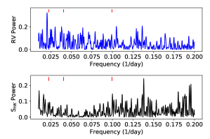
Figure 4: K2-3: periodograms of the radial velocity data (top) and $S_{\mathrm{HK}}$ (bottom). The three planet periods are shown by red tick marks at the top of the figures. The RV and $S_{\mathrm{HK}}$ periodogram do not have similar prominent peaks. Although the planet periods are not all visible in the RV periodogram due to their meter per second RV amplitudes, we are able to detangle the planet signals in the RV data by constraining the periods and conjunction times from K2 and Spitzer transits.

As mentioned above, $S_{\mathrm{HK}}$ may be a poor indicator for M-dwarf stars. To better characterize the possible rotation signal of K2-3, we analyzed photometry from the Evryscope. The Evryscope is an array of 24 61mm telescopes together imaging 8000 square degrees of sky every two minutes (Law et al., 2015). Since its 2015 installation at Cerro Tololo Inter-American Observatory (CTIO) in Chile, the Evryscope has observed on over 500 clear nights, tracking the sky for two hours at a time before ratcheting back and continuing observations, for an average of $\sim$6 hours of continuous monitoring each night. The Evryscope observes in Sloan-$g$’ at a resolution of 13”/pixel. High-cadence photometry of K2-3 is included in the Evryscope light curve database from 2016 January to 2018 March (Figure 5). Because K2-3 is in the northernmost region of the Evryscope field of view, the coverage of the target is limited each year, resulting in a total of $10^{4}$ epochs; most southern stars are observed with 4–6$\times$ more points.

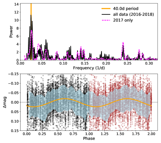
Figure 5: Evryscope photometry of K2-3, consisting of 9931 epochs at 2 minute cadence in Sloan-g’ from 2016 Jan to 2018 March. Top panel: the LS periodogram of K2-3 displays significant power around 40 days (orange line). A purple dashed line shows the power of only the 2017 photometry as a secondary confirmation. Bottom panel: phase-folded light curve folded over 40 days. The phase is repeated to guide the eye, and points are binned to eight-minute cadence to improve precision on this relatively faint Evryscope target. The 1$\sigma$ region about the mean of the phased lightcurve is shown (light blue area), along with a 40-day sinusoid with a characteristic amplitude of 0.02 mag (orange curve).

Evryscope light curves are generated using a custom pipeline. The Evryscope image archive contains 2.5 million raw images, $\sim$250TB of total data. Each image, consisting of a 30MPix FITS file from one camera, is dark-subtracted, flat-fielded and then astrometrically calibrated using a custom wide-field solver. Large-scale background gradients are removed, and forced-aperture photometry is then extracted based on known source positions in a reference catalog. Light curves are generated for approximately 15 million sources across the southern sky by differential photometry in small sky regions using carefully selected reference stars; residual systematics are removed using two iterations of the SysRem detrending algorithm. For 10th mag stars, this process results in $\approx$1% photometric stability at two-minute cadence when measured in multiple-year light curves over all sky conditions; co-adding produces improved precisions, down to $\sim$6 mmag.

Evryscope collected 9931 epochs of K2-3 at two-minute cadence in Sloan-$g$’ from 2016 January 2016 to 2018 March. The data were analyzed using a Lomb-Scargle (LS) periodogram to determine the likely rotation period of K2-3 (Figure 5). The highest peak is at 40.0 days, but power from the central peak is split due to the inter-year window function, verified by injecting similar signals to K2-3 and other nearby stars. An alias of the 40.0 day signal exists at a reduced power near 20 days. The periodogram for only the 2017 photometry produces a peak signal of 38 days. A signature of evolving starspot activity due to differential rotation near 40 days may explain this difference. The 40.0 day period shows a sinusoidal variation with a 0.02 mag variation. Therefore, we infer the rotation period of K2-3 to be 40 $\pm$ 2 days from the Evryscope data. Both the 2017 and the all-data rotation periods agree with the estimate from K2 data, within measurement errors. We use the Evryscope photometry to inform our GP priors in the RV fit (Section 4.3.2).

4.2.2 GJ3470 Stellar Activity

Figure 6: Top: Photometry of GJ3470 from 2012 to 2017 from the C14 AIT at Fairborn Observatory. Middle: Power spectrum of the observations in frequency space resulted in a stellar rotation period of 21.54 days. We inflated the period uncertainty to 21.54 $\pm$ 0.49 days, to account for the variation in rotation period over time. Bottom: Phased photometry over the periodogram peak at 21.54 days.

Table 6: Summary of C14 AIT Photometric Observations of GJ3470

Observing	Date Range		Sigma	Seasonal Mean
Season	(HJD$-$2,400,000)	$N_{obs}$	(mag)	(mag)
2012-2013	56272–56440	297	0.00535	$-0.99917\pm 0.00031$
2013-2014	56551–56813	289	0.00397	$-1.00205\pm 0.00023$
2014-2015	56949–57180	108	0.00419	$-1.00494\pm 0.00040$
2015-2016	57323–57508	83	0.00384	$-1.00214\pm 0.00042$
2016-2017	57705–57879	65	0.00586	$-1.00417\pm 0.00073$

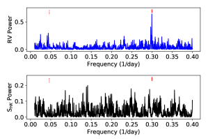
Figure 7: GJ3470: periodogram of the radial velocity data (top) and $S_{\mathrm{HK}}$ periodogram (bottom). The main peak in RV at 3.3 days matches the period of planet b (red tick mark). The next prominent peaks are near the stellar rotation period (red dotted mark; see Figure 6). The RV and $S_{\mathrm{HK}}$ periodograms do not have any prominent peaks in common.

To better characterize GJ3470, photometry was collected at the Fairborn Observatory in Arizona with the Tennessee State University Celestron C14 0.36 m Automated Imaging Telescope (AIT) (Henry, 1999; Eaton et al., 2003). The AIT has a SBIG STL-1001E CCD camera and a Cousins R filter. Images were corrected for bias, flat-fielding, and differential extinction. Differential magnitudes were computed using five field stars. 842 observations were collected from 2012 December to 2017 May (Table 6, Figure 6).

The tallest peak in the periodogram (Figure 6) corresponds to a period of 21.54 $\pm$ 0.49 days; the uncertainty is the standard deviation between the peaks for each observing season. We interpret this peak as the stellar rotation period, as shown by the brightness variation from star spots rotating in and out of view. This rotation period is consistent with that found by Biddle et al. (2014).

For GJ3470, there is a hint of an RV-$S_{\mathrm{HK}}$ correlation in the early HIRES data, although the full dataset has a correlation coefficient of -0.0753 and $p$-value of 0.5812. Furthermore, the RV periodogram contains a significant peak near the stellar rotation period (Figure 7), which suggests that the stellar rotation signal needs to be accounted for in the RV analysis. We therefore used this photometry to inform our GP priors in the RV fit (Section 4.3.1).

4.3 RV Analysis

We analyzed the RV data for both systems using RadVel, an open-source orbit-fitting toolkit for RV data (Fulton et al., 2018). RadVel models the RVs as the sum of Keplerian orbits. The model parameters are orbital period (P), time of inferior conjunction (T_conj), radial velocity amplitude (K), eccentricity ($e$), argument of periastron ($\omega$), a constant RV offset ($\gamma$), and a jitter term for each instrument ($\sigma$). In order to avoid biasing eccentricity, $\sqrt{e}cos(\omega)$ and $\sqrt{e}sin(\omega)$ are used as fitting parameters.

We modeled the correlated noise introduced from the stellar activity using a quasi-periodic Gaussian Process (GP) with a covariance kernel of the form

$$k(t,t^{\prime})=\eta_{1}^{2}\ \rm{exp}\left[-\frac{(t-t^{\prime})^{2}}{\eta_{2}^{2}}-\frac{sin^{2}(\frac{\pi(t-t^{\prime})}{\eta_{3}})}{\eta_{4}^{2}})\right],$$ (1)

where the hyper-parameter $\eta_{1}$ is the amplitude of the covariance function, $\eta_{2}$ is the active region evolutionary time scale, $\eta_{3}$ is the period of the correlated signal, and $\eta_{4}$ is the length scale of the periodic component (López-Morales et al., 2016; Haywood et al., 2014). We trained these parameters on the ground-based photometry of each star by performing a maximum likelihood fit to the associated ground-based light curve with the quasi-periodic kernel (Eq. 1) then determined the errors through a MCMC analysis. We then compare the period of the correlated signal ($\eta_{3}$) with the stellar rotation period found from our periodogram analysis in Section 4.2.

4.3.1 GJ3470 RV Analysis

For our RV analysis of GJ3470, we adopt the period, time of conjunction, and planet radius derived from a variety of ground-based telescopes (Biddle et al., 2014). The remaining parameters were initialized from Dragomir et al. (2015).

We used a GP to model the correlated noise associated with the stellar activity in our RV fit. We ran our GP analysis on the photometry from Fairborn Observatory (FO, Section 4.2) and find $\gamma_{FO}$ = $1.003\pm 0.001$, $\sigma_{FO}$ = $0.0029\pm 0.0001$, $\eta_{1}$ = $-0.0036^{+0.0003}_{-0.0004}$, $\eta_{2}$ = $48.98^{+9.54}_{-7.28}$, $\eta_{3}$ = $21.84^{+0.35}_{-0.36}$, and $\eta_{4}$ = $0.55\pm 0.06$. This stellar rotation period ($\eta_{3}$) is consistent with the results of our periodogram analysis in Section 4.2 to within 1$\sigma$.

We then perform our RV fit including a GP modeled as a sum of two quasi-periodic kernels, one for each instrument, as HIRES and HARPS have different properties that could alter the effect of stellar activity on the data. Each kernel includes identical $\eta_{2}$, $\eta_{3}$, and $\eta_{4}$ parameters but allows for different $\eta_{1}$ values. Our priors are as follows: $\eta_{1}$ is left as a free parameter as light curve amplitude cannot be directly translated to RV amplitude, for $\eta_{2}$, $\eta_{3}$, and $\eta_{4}$, we used a kernel density estimate (KDE) of the Fairborn Observatory photometry posteriors.

After running an initial RV fit including only one circular, Keplerian planet signal, we investigated models including an acceleration term, curvature term, and eccentricity. The Aikike information criterion (AIC) was used to determine if the fit improvement justified the additional parameters; a $\Delta$AIC of $<$ 2 indicates a similar fit, 2 $<$ $\Delta$AIC$<$ 10 favors the additional parameter, and a $\Delta$AIC $>$ 10 is a strong justification for the additional parameter. Only the eccentricity parameters improved the AIC ($\Delta$AIC_acc = -0.71, $\Delta$AIC_curv = -1.44, and $\Delta$AIC_ecc = 6.45). All of the tested RV models resulted in planet masses within 1$\sigma$ of the circular fit values shown in Table 7

We then investigated a model including an eccentricity constraint from Spitzer observations of the secondary eclipse. The secondary eclipse was 0.309 days later than expected for a circular orbit, which results in a constraint on $e$cos$(\omega)$ of $0.014546^{+0.000753}_{-0.000659}$ (Benneke, in review). For this fit we used $e$cos$(\omega)$ and $e$sin$(\omega)$ as the fitting basis due to the prior set by the secondary eclipse. We find an eccentricity of $e_{b}=0.114\pm 0.051$ for the eccentric model constrained by this secondary eclipse measurement, the best-fit curve is shown in Figure 8.

The non-zero eccentricity value of GJ3470 b is particularly interesting in the context of other systems. GJ436 b, another planet similar in mass, radius, period, and stellar host, has a puzzlingly high eccentricity of 0.150 $\pm$ 0.012 (Deming et al., 2007). These high eccentricity values may be an emerging clue on how these types of planets form and migrate.

Table 7: GJ3470 RV MCMC Priors and Posteriors

Parameter	Value	Units
Gaussian Priors
$T\rm{conj}_{b}$	$2455953.6645\pm 0.0034$	JD
$P_{b}$	$3.3371\pm 0.0002$	days
$e\cos{\omega}_{b}$	$0.01454\pm 0.00075323$
$\eta_{1,HIRES}$	[0,100]	m s-1
$\eta_{1,HARPS}$	[0,100]	m s-1
$\eta_{2}$	$48.98^{+9.54}_{-7.28}$	days
$\eta_{3}$	$21.84^{+0.35}_{-0.36}$	days
$\eta_{4}$	$0.55\pm 0.006$
Orbital Parameters
$P_{b}$	$3.336649^{+8.4e-05}_{-8.1e-05}$	days
$T\rm{conj}_{b}$	$2455953.663\pm 0.0035$	JD
$e_{b}$	$0.114^{+0.052}_{-0.051}$
$\omega_{b}$	$-1.44^{+0.1}_{-0.04}$	radians
$K_{b}$	$8.21^{+0.47}_{-0.46}$	m s-1
$M_{b}$	$12.58^{+1.31}_{-1.28}$	M⊕
$\rho_{b}$	$0.93^{+0.56}_{-0.31}$	g cm-3
Other Parameters
$\gamma_{\rm HIRES}$	$0.3^{+1.2}_{-1.1}$	m s-1
$\gamma_{\rm HARPS}$	$26500.52^{+0.59}_{-0.6}$	m s-1
$\dot{\gamma}$	$\equiv$ 0.0	m s-1 day-1
$\ddot{\gamma}$	$\equiv$ 0.0	m s-1 day-2
$\sigma_{\rm HIRES}$	$1.9^{+0.7}_{-0.67}$	$\rm m\ s^{-1}$
$\sigma_{\rm HARPS}$	$0.0023^{+0.49}_{-0.0023}$	$\rm m\ s^{-1}$
$\eta_{1,HIRES}$	$3.94^{+0.90}_{-0.78}$	m s-1
$\eta_{1,HARPS}$	$1.79^{+0.69}_{-0.71}$	m s-1
$\eta_{2}$	$49.40^{+10.00}_{-7.55}$	days
$\eta_{3}$	$21.92^{+0.42}_{-0.41}$	days
$\eta_{4}$	$0.56\pm 0.06$

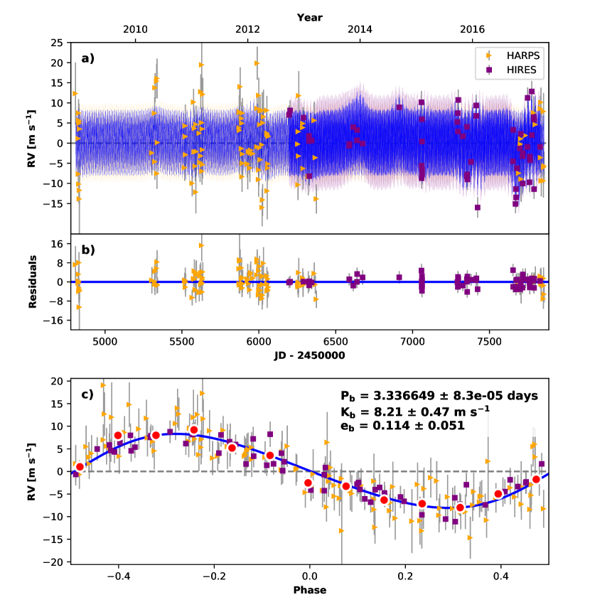
Figure 8: Best-fit one-planet Keplerian orbital model for GJ3470 with $e$cos$(\omega)$ constraints from the secondary eclipse observation. The maximum likelihood model is plotted while the orbital parameters listed in Table 7 are the median values of the posterior distributions. The thin blue line is the best fit one-planet model with the mean GP model; the colored area surrounding this line includes the 1$\sigma$ maximum likelihood GP uncertainties. We add in quadrature the RV jitter term(s) listed in Table 7 with the measurement uncertainties for all RVs. b) Residuals to the best-fit one-planet model. c) RVs phase-folded to the ephemeris of planet b. The small point colors and symbols are the same as in panel a). The red circles are the same velocities binned in 0.08 units of orbital phase.

4.3.2 K2-3 RV analysis

For our RV analysis of K2-3, we adopt the planet orbital periods and times of conjunction from our Spitzer analysis (Section 3). We used a GP to model the correlated noise associated with the stellar activity in our RV fit. We ran our GP analysis on the photometry from Evryscope (ES, Section 4.2) and find $\gamma_{ES}$ = $11.61\pm 0.01$, $\sigma_{ES}$ = $0.017^{+0.004}_{-0.003}$, $\eta_{1}$ = $0.03\pm 0.01$, $\eta_{2}$ = $44.57^{+12.58}_{-16.23}$, $\eta_{3}$ = $37.80^{+1.77}_{-2.04}$, and $\eta_{4}$ = $0.47\pm 0.05$. This stellar rotation period ($\eta_{3}$) is consistent with the results of our periodogram analysis in Section 4.2 to within 2-$\sigma$.

We then perform our RV fit including a GP modeled as a sum of four quasi-periodic kernels, one for HIRES, HARPS, HARPS-N and PFS, as described above for GJ3470. Our GP hyperparameter priors are as follows: $\eta_{1}$ is left as a free parameter as light curve amplitude cannot be directly translated to RV amplitude. To construct priors on $\eta_{2}$, $\eta_{3}$, and $\eta_{4}$, we use a KDE of the Evryscope photometry posteriors.

After running an initial RV fit including only three circular, Keplerian planet signals, we investigated additional models including an acceleration term, curvature term, and planet eccentricity. The fit including an additional term for acceleration, curvature, and eccentricity had $\Delta$AIC of -2.17, -2.22, and -2.92 respectively; none of these justified the additional parameter.  Table 8 shows the MCMC priors, orbital parameters, and statistics for the GP model of K2-3. The best-fit curves for each planet is shown in Figure 9.

Table 8: K2-3 RV MCMC Priors and Posteriors

Parameter	Three-Planet Fit	Units
Gaussian Priors
$T\rm{conj}_{b}$	$2456813.41843\pm 0.00039$	JD
$P_{b}$	$10.054626\pm 1e-05$	days
$T\rm{conj}_{c}$	$2456812.28013\pm 0.00095$	JD
$P_{c}$	$24.646582\pm 3.9e-05$	days
$T\rm{conj}_{d}$	$2456826.22347\pm 0.00053$	JD
$P_{d}$	$44.556456\pm 9.7e-05$	days
$\eta_{1,all}$	[0,100]	m s-1
$\eta_{2}$	$44.57^{+12.58}_{-16.23}$	days
$\eta_{3}$	$37.80^{+1.77}_{-2.04}$	days
$\eta_{4}$	$0.47\pm 0.05$
Orbital Parameters
$P_{b}$	$10.054626^{+1e-05}_{-1.1e-05}$	days
$T\rm{conj}_{b}$	$2456813.41843\pm 0.00041$	JD
$e_{b}$	$\equiv$ 0.0
$\omega_{b}$	$\equiv$ 0.0	radians
$K_{b}$	$2.72^{+0.29}_{-0.3}$	m s-1
$M_{b}$	$6.48^{+0.99}_{-0.93}$	M⊕
$\rho_{b}$	$3.70^{+1.67}_{-1.08}$	g cm-3
$P_{c}$	$24.646582^{+4.1e-05}_{-4e-05}$	days
$T\rm{conj}_{c}$	$2456812.28018^{+0.00098}_{-0.001}$	JD
$e_{c}$	$\equiv$ 0.0
$\omega_{c}$	$\equiv$ 0.0	radians
$K_{c}$	$0.67\pm 0.32$	m s-1
$M_{c}$	$2.14^{+1.08}_{-1.04}$	M⊕
$\rho_{c}$	$2.98^{+1.96}_{-1.50}$	g cm-3
$P_{d}$	$44.55646^{+0.00011}_{-0.0001}$	days
$T\rm{conj}_{d}$	$2456826.22346\pm 0.00056$	JD
$e_{d}$	$\equiv$ 0.0
$\omega_{d}$	$\equiv$ 0.0	radians
$K_{d}$	$-0.13^{+0.28}_{-0.31}$	m s-1
$M_{d}$	$-0.50^{+1.10}_{-1.20}$	M⊕
$\rho_{d}$	$-0.98^{+2.20}_{-2.83}$	g cm-3
$K_{d}$ (3$\sigma$ upper)	$0.71$	m s-1
$M_{d}$ (3$\sigma$ upper)	$2.80$	M⊕
$\rho_{d}$ (3$\sigma$ upper)	$5.62$	g cm-3
Other Parameters
$\gamma_{\rm PFS}$	$-1.3\pm 2.2$	m s-1
$\gamma_{\rm HIRES}$	$-2.98^{+0.97}_{-1.0}$	m s-1
$\gamma_{\rm HARPS-N}$	$0.53^{+0.71}_{-0.74}$	$\rm m\ s^{-1}$
$\gamma_{\rm HARPS}$	$-0.59^{+0.69}_{-0.73}$	m s-1
$\dot{\gamma}$	$\equiv$ 0.0	m s-1 day-1
$\ddot{\gamma}$	$\equiv$ 0.0	m s-1 day-2
$\sigma_{\rm PFS}$	$4.85^{+1.0}_{-0.88}$	$\rm m\ s^{-1}$
$\sigma_{\rm HIRES}$	$2.98^{+0.47}_{-0.42}$	$\rm m\ s^{-1}$
$\sigma_{\rm HARPS-N}$	$1.61^{+0.26}_{-0.25}$	$\rm m\ s^{-1}$
$\sigma_{\rm HARPS}$	$2.06^{+0.34}_{-0.32}$	$\rm m\ s^{-1}$
$\eta_{1,PFS}$	$4.75^{+3.72}_{-2.58}$	m s-1
$\eta_{1,HIRES}$	$3.21^{+0.84}_{-0.73}$	m s-1
$\eta_{1,HARPS}$	$3.04^{+0.64}_{-0.53}$	m s-1
$\eta_{1,HARPS-N}$	$3.07^{+0.61}_{-0.48}$	m s-1
$\eta_{2}$	$62.25^{+10.78}_{-9.84}$	days
$\eta_{3}$	$39.16^{+0.88}_{-0.96}$	days
$\eta_{4}$	$0.41^{+0.05}_{-0.04}$

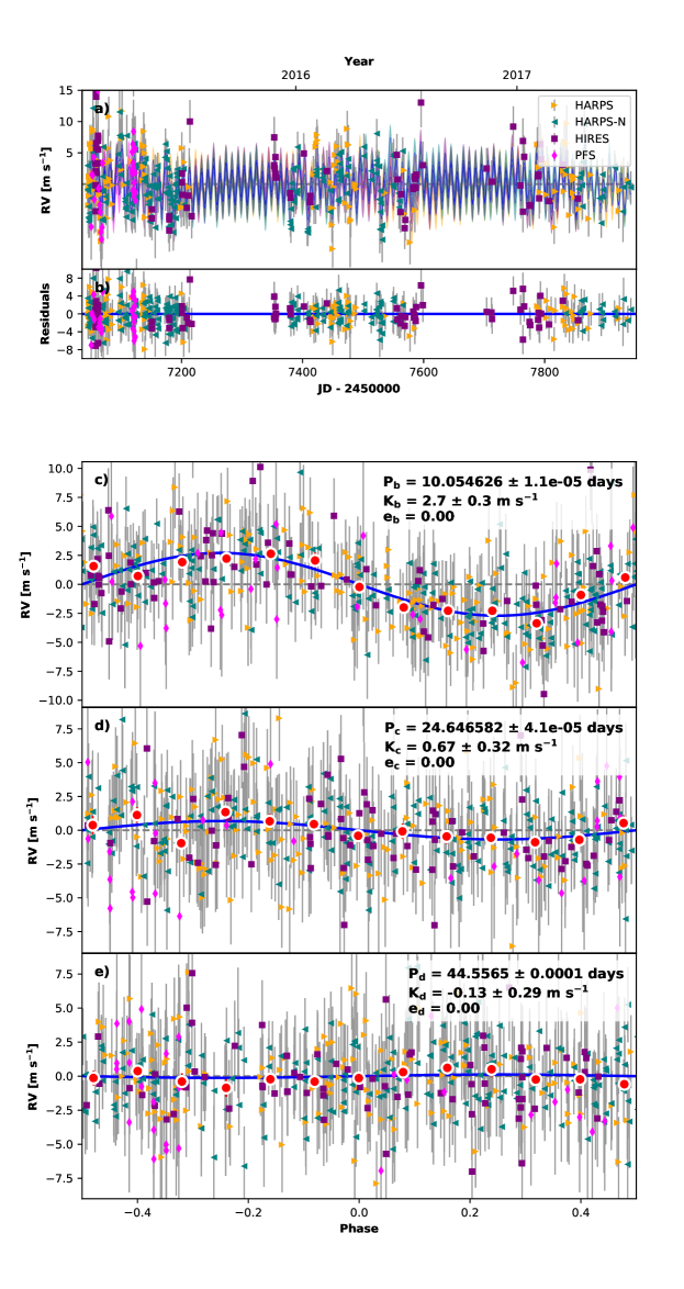
Figure 9: Best-fit three-planet Keplerian orbital model for K2-3. The maximum likelihood model is plotted while the orbital parameters listed in Table 8 are the median values of the posterior distributions. The thin blue line is the best-fit three-planet model with the mean GP model; the colored area surrounding this line includes the 1-$\sigma$ maximum likelihood GP uncertainties. We add in quadrature the RV jitter term(s) listed in Table 8 with the measurement uncertainties for all RVs. b) Residuals to the best-fit three-planet model. c) RVs phase-folded to the ephemeris of planet b. The Keplerian orbital models for all other planets have been subtracted. The small point colors and symbols are the same as in panel a). The red circles are the same velocities binned in 0.08 units of orbital phase. The phase-folded model for planet b is shown as the blue line. Panel d) and e) are the same as panel c) but for planet K2-3 c and d, respectively.

From our GP fit, we find that the semi-amplitude of the signal from planet d is consistent with 0 to 1$\sigma$. It is possible that this planet has a small semi-amplitude (K_d $<<$ m s^-1) and we were unable to detect it. Alternatively, as the period of planet d (P_d = 44.56 days) is near the stellar rotation period ($\eta_{3}\approx$ 40 days), it is possible that the signal of planet d is indistinguishable from the stellar activity signal. Further work is needed to distinguish between the two possibilities and determine the mass of planet d.

5 Discussion

These four Earth- to Neptune-sized planets are great candidate targets for atmospheric transmission spectroscopy due to their bright host stars (K $<$ 9 mag) and low densities ($<4.2$ g cm^-3). GJ3470 b has been observed with the Hubble Space Telescope (HST) in cycles 19 and 22 (GO 13064, GO 13665). K2-3 d and the K2-3 UV emission will be observed in cycles 24 and 25 (GO 14682, GO 15110). GJ3470 b already shows H₂O absorption (Tsiaras et al. (2017); Benneke et al. 2018, submitted) and is being targeted by JWST Guaranteed Time Observation (GTO) program observations.

It is important to characterize potential targets to determine precise mass and surface gravity measurements, as these parameters will affect the interpretation of future transmission spectroscopy observations. We examined the potential atmospheric composition of these planets in two ways. First, we investigate their potential compositions in a mass-radius diagram (Figure 10). Fulton et al. (2017) describes a bimodality in occurrence rates of small planets in terms of planet radius with a gap between 1.5 and 2.0 R_⊕. This distribution in radius suggests a similar distribution in planet composition, where planets smaller than 1.5 R_⊕ are super-Earths and planets 2.0–3.0 R_⊕ are sub-Neptunes. The three K2-3 planets fall in three different places relative to the radius gap (Fulton et al., 2017); planet b lies above, planet c is within the gap, and planet d is just below.

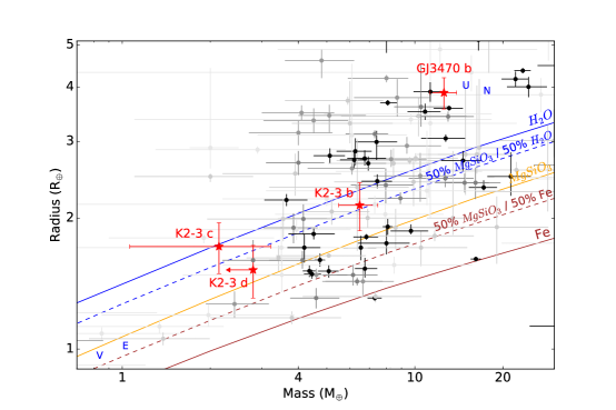
Figure 10: Mass-radius diagram for planets between the size of Earth and Neptune (darker points for smaller error). The compositional curves listed are theoretical models (Zeng et al., 2016) for planets with an iron (brown), silicate (orange), and water (blue) composition. K2-3 b, c, and GJ3470 b (red stars) are shown with 1$\sigma$ uncertainties along with the K2-3 d 3$\sigma$ upper limit on mass. All four planets likely have volatile-rich envelopes.

We examine the bulk composition of these four planets in the context of other super-Earth and sub-Neptune planets (Figure 10). GJ3470 b occupies the same mass-radius space as our own ice giants, Uranus and Neptune, and likely also has a substantial volatile envelope. Depending on its core composition, GJ3470 b has between 4% and 13% H/He (Lopez & Fortney, 2014). K2-3 b and c both have a bulk density consistent with a mixture of silicates and water. As a water planet is an unlikely product of planet formation, they likely have iron-silicate cores with a small volatile envelope. Assuming an Earth-like core, K2-3 b and c both have about 0.5% H/He by mass (Lopez & Fortney, 2014). However, K2-3 c is also consistent with no volatile atmosphere given a sufficient amount of lighter material in the core, and the 3$\sigma$ mass measurement is consistent with an Earth-like composition. K2-3 d is potentially the lightest planet compared to others of similar radii; it needs substantial volatiles to explain it’s placement on the mass-radius diagram. The two main interpretations are: (1) the planet is sufficiently low-mass to not detect its signal, requiring a significant volatile percentage, or (2) we have not adequately accounted for the stellar activity RV signal in this analysis, therefore, the actual mass of planet d is higher than listed here.

Our mass measurements of K2-3 b and c are within 1$\sigma$ of Almenara et al. (2015) and Dai et al. (2016). Our mass measurement of K2-3 d is within 3$\sigma$ of Dai et al. (2016) and 4$\sigma$ of Almenara et al. (2015). Our measurements of K2-3 b is within 1$\sigma$ of Damasso et al. (2018), K2-3 c is within 2$\sigma$, and K2-3 d is within 2$\sigma$ of their RV fit and within 3$\sigma$ of their injection/recovery tests. We have improved the precision of the mass measurement of all three planets compared to previous measurements. However, due to the potential stellar activity contamination, use caution with the measurement for K2-3 d.

We then simulated model transmission spectra for the K2-3 planet system using ExoTransmit (Kempton et al., 2017) to examine their possible atmospheric compositions (Figure 11). Two spectra were created for planet b and c according to the 1$\sigma$ lower and upper bounds on the mass. Two spectra were created for planet d according to the upper 2$\sigma$ and upper 3$\sigma$ mass, as the mass measurement is consistent with zero. Our assumptions include no clouds, chemical equilibrium, a 100 M/H ratio, and the 1 bar radius equals the transit radius.

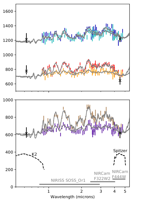
Figure 11: Simulated transmission spectra (grey) of K2-3 b (blue/green, top) and c (red/orange, middle) for their 1$\sigma$ low-mass and high-mass cases and spectra for K2-3 d (brown/purple, bottom) for the upper 1$\sigma$ and 2-$\sigma$ cases. The error bars refer to simulated JWST observations with PandExo (Batalha et al., 2017b). K2 and Spitzer datapoints and bandpasses are shown in black. JWST instrument wavelength ranges are shown in grey. Note the break in the y-axis used for clarity.

The transit depth was adjusted to match the K2 (Crossfield et al., 2015a) and Spitzer transit depths. Simulated JWST observations and error bars are superimposed on top of the spectra using PandExo (Greene et al., 2016; Batalha et al., 2017b). We simulated one transit for each planet with three instrument modes: NIRCam F332W2, NIRCam F444W, and NIRISS SOSS_Or1. We used the Phoenix grid models to simulate a stellar spectrum with a magnitude of 8.56 $K$ mag, temperature of 3890 K, metallicity of 0.3, and log(g) of 4.8. For each transit, we included a baseline of equal time to the transit time, zero noise floor, and resolution of R = 35.

For K2-3 b, the absorption features would be observable for a true mass value within 1$\sigma$ of our mass measurement; the light and dark blue simulated datapoints are both inconsistent with a flat spectra. From this, K2-3 b is particularly a good target for future atmospheric study. For K2-3 c, the absorption features would be easily observable for a mass on the lower 1$\sigma$ side of our measurement, but would be much more difficult for the higher mass case. Lastly, K2-3 d would have distinguishable features as long as the mass is lower than our 2$\sigma$ upper limit.

The Spitzer transit depths for K2-3 c and d are quite similar (Figure 2) although their K2 transit depths are considerably offset. Beichman et al. (2016a) also find similar Spitzer transit depths for K2-3 c and d. We were unable to create a model spectra for planet c that was consistent with both the K2 and Spitzer data to 1$\sigma$. However, this model did not include clouds, which could improve the fit of the model to the data (Sing et al., 2016).

Transmission spectra can help to constrain a planet’s mass further as the scale height depends on the planet’s gravity (de Wit & Seager, 2013). However, one must be careful as there are significant degeneracies between the effects of mass and composition for small planets (Batalha et al., 2017a). With the mass of the planets constrained here through the RV method, further constraints can be put on the atmospheric composition from the transmission spectra.

These planets are example training cases for future TESS planets. TESS will find a large sample of bright systems around nearby stars (Ricker et al., 2014; Sullivan et al., 2015; Ballard, 2018). These types of planets will be ideal for JWST atmospheric observations due to their bright host stars. Prior to transmission spectroscopy observations, these systems will need to be followed up in a similar method as described in this paper to determine the planet masses in order to correctly interpret the spectra.

6 Conclusion

In summary, we report improved masses, radii, and densities for four planets in two systems, K2-3 and GJ3470, derived from a combination of new RV, photometry, and transit observations. Our primary results are as follows.

Transit follow-ups are key for refining planet ephemerides sufficiently for future characterization. Extending the observation baseline with Spitzer greatly narrows the projected transit window. Our uncertainties are 20 times smaller than the original K2 data, which decreases the 3$\sigma$ uncertainty in the JWST era for planet d from $\sim$25 hours to under 30 minutes (Figure 3). Our additional Spitzer data improve the ephemeris for the K2-3 planets to one-thirds that of Beichman et al. (2016a). See Section 3 for our Spitzer analysis and discussion.

$S_{\mathrm{HK}}$ may not be a good indicator for stellar activity in M dwarfs. For GJ3470, there was little to no correlation between the RVs and $S_{\mathrm{HK}}$; however, the rotation period found by our photometric monitoring was present in our RV data. For K2-3, although there was no correlation with $S_{\mathrm{HK}}$, our Evryscope photometry showed clear periodicity near the orbital period of K2-3d. Photometry and H$\alpha$ can be useful diagnostics for M-dwarf stellar rotation periods instead of $S_{\mathrm{HK}}$ (Newton et al., 2017; Robertson et al., 2015; Damasso et al., 2018). See Sections 4.2.1 and 4.2.2 for a description of our $S_{\mathrm{HK}}$ values and stellar activity discussion.

Photometric monitoring of planet-hosting stars is important to determine the stellar rotation period and spot modulation to therefore separate the stellar activity from the planet-induced RV signals. This is especially important for planetary systems with low-amplitude RV signals as these signals may be hidden by stellar activity. We used a GP trained on our photometry to increase the accuracy of our RV fits. See Section 4.3 for our RV analysis including this GP.

From our radial velocity analysis, we determined the mass of GJ3470 b to nearly ten sigma (M_b = $12.58^{+1.31}_{-1.28}$ M_⊕), see Section 4.3.1. We additionally constrained the planet eccentricity ($e_{b}$ = 0.114${}^{+0.52}_{-0.51}$) from our RV analysis and a measured secondary eclipse from Spitzer. Non-zero eccentricities may be an emerging clue on how warm-Neptunes form and migrate.

We have determined an upper limit on the mass of K2-3 d of 2.80 M_⊕. With such a low mass, this planet is consistent with having a substantial volatile envelope which decreases its chance for habitability. As such, K2-3 likely hosts three sub-Neptune planets instead of super-Earth planets. These planets present an interesting case for transmission spectroscopy observations of temperate sub-Neptunes. See Section 5 for simulated transmission spectra of these three planets.

References

- Almenara et al. (2015) Almenara, J. M., Astudillo-Defru, N., Bonfils, X., et al. 2015, A&A, 581, L7
- Astudillo-Defru et al. (2015) Astudillo-Defru, N., Bonfils, X., Delfosse, X., et al. 2015, A&A, 575, A119
- Astudillo-Defru et al. (2017) Astudillo-Defru, N., Forveille, T., Bonfils, X., et al. 2017, A&A, 602, A88
- Ballard (2018) Ballard, S. 2018, ArXiv e-prints, arXiv:1801.04949
- Batalha et al. (2017a) Batalha, N. E., Kempton, E. M.-R., & Mbarek, R. 2017a, ApJ, 836, L5
- Batalha et al. (2017b) Batalha, N. E., Mandell, A., Pontoppidan, K., et al. 2017b, PASP, 129, 064501
- Beichman et al. (2016a) Beichman, C., Livingston, J., Werner, M., et al. 2016a, ApJ, 822, 39
- Beichman et al. (2016b) —. 2016b, ApJ, 822, 39
- Benneke (in review) Benneke, B. in review
- Benneke et al. (2017) Benneke, B., Werner, M., Petigura, E., et al. 2017, ApJ, 834, 187
- Biddle et al. (2014) Biddle, L. I., Pearson, K. A., Crossfield, I. J. M., et al. 2014, MNRAS, 443, 1810
- Bodenheimer & Lissauer (2014) Bodenheimer, P., & Lissauer, J. J. 2014, ApJ, 791, 103
- Bonfils et al. (2012) Bonfils, X., Gillon, M., Udry, S., et al. 2012, A&A, 546, A27
- Bourrier et al. (2018) Bourrier, V., Lecavelier des Etangs, A., Ehrenreich, D., et al. 2018, A&A, 620, A147
- Bradley et al. (2016) Bradley, L., Sipocz, B., Robitaille, T., et al. 2016, astropy/photutils: v0.3, , , doi:10.5281/zenodo.164986
- Buccino et al. (2011) Buccino, A. P., Díaz, R. F., Luoni, M. L., Abrevaya, X. C., & Mauas, P. J. D. 2011, AJ, 141, 34
- Chen et al. (2017) Chen, G., Guenther, E. W., Pallé, E., et al. 2017, A&A, 600, A138
- Cincunegui et al. (2007) Cincunegui, C., Díaz, R. F., & Mauas, P. J. D. 2007, A&A, 469, 309
- Claret et al. (2012a) Claret, A., Hauschildt, P. H., & Witte, S. 2012a, VizieR Online Data Catalog, 354
- Claret et al. (2012b) —. 2012b, VizieR Online Data Catalog, 354
- Crossfield et al. (2013) Crossfield, I. J. M., Barman, T., Hansen, B. M. S., & Howard, A. W. 2013, A&A, 559, A33
- Crossfield et al. (2015a) Crossfield, I. J. M., Petigura, E., Schlieder, J. E., et al. 2015a, ApJ, 804, 10
- Crossfield et al. (2015b) —. 2015b, ApJ, 804, 10
- Crossfield et al. (2016) Crossfield, I. J. M., Ciardi, D. R., Petigura, E. A., et al. 2016, ApJS, 226, 7
- Cutri et al. (2003) Cutri, R. M., Skrutskie, M. F., van Dyk, S., et al. 2003, VizieR Online Data Catalog: 2MASS All-Sky Catalog of Point Sources (Cutri+ 2003), Vol. 2246
- Dai et al. (2016) Dai, F., Winn, J. N., Albrecht, S., et al. 2016, ApJ, 823, 115
- Damasso et al. (2018) Damasso, M., Bonomo, A. S., Astudillo-Defru, N., et al. 2018, ArXiv e-prints, arXiv:1802.08320
- de Wit & Seager (2013) de Wit, J., & Seager, S. 2013, Science, 342, 1473
- Deming et al. (2007) Deming, D., Harrington, J., Laughlin, G., et al. 2007, ApJ, 667, L199
- Deming et al. (2015) Deming, D., Knutson, H., Kammer, J., et al. 2015, ApJ, 805, 132
- Demory et al. (2013) Demory, B.-O., Torres, G., Neves, V., et al. 2013, ApJ, 768, 154
- Dragomir et al. (2015) Dragomir, D., Benneke, B., Pearson, K. A., et al. 2015, ApJ, 814, 102
- Dressing & Charbonneau (2013) Dressing, C. D., & Charbonneau, D. 2013, ApJ, 767, 95
- Dressing & Charbonneau (2015) —. 2015, ApJ, 807, 45
- Dressing et al. (2017) Dressing, C. D., Vanderburg, A., Schlieder, J. E., et al. 2017, AJ, 154, 207
- Eaton et al. (2003) Eaton, J. A., Henry, G. W., & Fekel, F. C. 2003, in Astrophysics and Space Science Library, Vol. 288, Astrophysics and Space Science Library, ed. T. D. Oswalt, 189
- Foreman-Mackey et al. (2013) Foreman-Mackey, D., Hogg, D. W., Lang, D., & Goodman, J. 2013, PASP, 125, 306
- Fressin et al. (2013) Fressin, F., Torres, G., Charbonneau, D., et al. 2013, ApJ, 766, 81
- Fukui et al. (2016) Fukui, A., Livingston, J., Narita, N., et al. 2016, AJ, 152, 171
- Fukui et al. (2013) Fukui, A., Narita, N., Kurosaki, K., et al. 2013, ApJ, 770, 95
- Fulton et al. (2018) Fulton, B. J., Petigura, E. A., Blunt, S., & Sinukoff, E. 2018, ArXiv e-prints, arXiv:1801.01947
- Fulton et al. (2017) Fulton, B. J., Petigura, E. A., Howard, A. W., et al. 2017, ArXiv e-prints, arXiv:1703.10375
- Gomes da Silva et al. (2012) Gomes da Silva, J., Santos, N. C., Bonfils, X., et al. 2012, A&A, 541, A9
- Goodman & Weare (2010) Goodman, J., & Weare, J. 2010, Communications in Applied Mathematics and Computational Science, Vol. 5, No. 1, p. 65-80, 2010, 5, 65
- Greene et al. (2016) Greene, T. P., Line, M. R., Montero, C., et al. 2016, ApJ, 817, 17
- Hayashi (1981) Hayashi, C. 1981, Progress of Theoretical Physics Supplement, 70, 35
- Haywood et al. (2014) Haywood, R. D., Collier Cameron, A., Queloz, D., et al. 2014, MNRAS, 443, 2517
- Henry (1999) Henry, G. W. 1999, PASP, 111, 845
- Howard et al. (2010) Howard, A. W., Johnson, J. A., Marcy, G. W., et al. 2010, ApJ, 721, 1467
- Howard et al. (2012) Howard, A. W., Marcy, G. W., Bryson, S. T., et al. 2012, ApJS, 201, 15
- Huber et al. (2016) Huber, D., Bryson, S. T., Haas, M. R., et al. 2016, ApJS, 224, 2
- Ingalls et al. (2016) Ingalls, J. G., Krick, J. E., Carey, S. J., et al. 2016, AJ, 152, 44
- Isaacson & Fischer (2010) Isaacson, H., & Fischer, D. 2010, ApJ, 725, 875
- Jones et al. (2001) Jones, E., Oliphant, T., Peterson, P., et al. 2001, SciPy: Open source scientific tools for Python, ,
- Kempton et al. (2017) Kempton, E. M.-R., Lupu, R., Owusu-Asare, A., Slough, P., & Cale, B. 2017, PASP, 129, 044402
- Kipping (2013) Kipping, D. M. 2013, MNRAS, 435, 2152
- Knutson et al. (2012) Knutson, H. A., Lewis, N., Fortney, J. J., et al. 2012, ApJ, 754, 22
- Kreidberg (2015) Kreidberg, L. 2015, PASP, 127, 1161
- Law et al. (2015) Law, N. M., Fors, O., Ratzloff, J., et al. 2015, PASP, 127, 234
- Lee & Chiang (2016) Lee, E. J., & Chiang, E. 2016, ApJ, 817, 90
- Lee et al. (2014) Lee, E. J., Chiang, E., & Ormel, C. W. 2014, ApJ, 797, 95
- Livingston et al. (2019) Livingston, J. H., Crossfield, I. J. M., Werner, M. W., et al. 2019, arXiv e-prints, arXiv:1901.05855
- Lopez & Fortney (2014) Lopez, E. D., & Fortney, J. J. 2014, ApJ, 792, 1
- López-Morales et al. (2016) López-Morales, M., Haywood, R. D., Coughlin, J. L., et al. 2016, AJ, 152, 204
- Mayo et al. (2018) Mayo, A. W., Vanderburg, A., Latham, D. W., et al. 2018, ArXiv e-prints, arXiv:1802.05277
- McQuillan et al. (2013) McQuillan, A., Aigrain, S., & Mazeh, T. 2013, MNRAS, 432, 1203
- Mizuno (1980) Mizuno, H. 1980, Progress of Theoretical Physics, 64, 544
- Montet et al. (2015) Montet, B. T., Morton, T. D., Foreman-Mackey, D., et al. 2015, ApJ, 809, 25
- Mulders et al. (2015) Mulders, G. D., Pascucci, I., & Apai, D. 2015, ApJ, 798, 112
- Nascimbeni et al. (2013) Nascimbeni, V., Piotto, G., Pagano, I., et al. 2013, A&A, 559, A32
- Newton et al. (2017) Newton, E. R., Irwin, J., Charbonneau, D., et al. 2017, ApJ, 834, 85
- Newton et al. (2016) Newton, E. R., Irwin, J., Charbonneau, D., Berta-Thompson, Z. K., & Dittmann, J. A. 2016, ApJ, 821, L19
- Ormel et al. (2017) Ormel, C. W., Liu, B., & Schoonenberg, D. 2017, A&A, 604, A1
- Petigura et al. (2013) Petigura, E. A., Howard, A. W., & Marcy, G. W. 2013, Proceedings of the National Academy of Science, 110, 19273
- Reid et al. (1997) Reid, I. N., Hawley, S. L., & Gizis, J. E. 1997, VizieR Online Data Catalog, 3198
- Ricker et al. (2014) Ricker, G. R., Winn, J. N., Vanderspek, R., et al. 2014, in Proc. SPIE, Vol. 9143, Space Telescopes and Instrumentation 2014: Optical, Infrared, and Millimeter Wave, 914320
- Robertson et al. (2013) Robertson, P., Endl, M., Cochran, W. D., & Dodson-Robinson, S. E. 2013, ApJ, 764, 3
- Robertson et al. (2015) Robertson, P., Endl, M., Henry, G. W., et al. 2015, ApJ, 801, 79
- Rogers (2015) Rogers, L. A. 2015, ApJ, 801, 41
- Sing et al. (2016) Sing, D. K., Fortney, J. J., Nikolov, N., et al. 2016, Nature, 529, 59
- Sullivan et al. (2015) Sullivan, P. W., Winn, J. N., Berta-Thompson, Z. K., et al. 2015, ApJ, 809, 77
- Swift et al. (2013) Swift, J. J., Johnson, J. A., Morton, T. D., et al. 2013, ApJ, 764, 105
- Tsiaras et al. (2017) Tsiaras, A., Waldmann, I. P., Zingales, T., et al. 2017, ArXiv e-prints, arXiv:1704.05413
- Van Eylen et al. (2017) Van Eylen, V., Agentoft, C., Lundkvist, M. S., et al. 2017, ArXiv e-prints, arXiv:1710.05398
- Vanderburg et al. (2016) Vanderburg, A., Latham, D. W., Buchhave, L. A., et al. 2016, ApJS, 222, 14
- Vogt et al. (1994) Vogt, S. S., Allen, S. L., Bigelow, B. C., et al. 1994, in Proc. SPIE, Vol. 2198, Instrumentation in Astronomy VIII, ed. D. L. Crawford & E. R. Craine, 362
- Weidenschilling (1977) Weidenschilling, S. J. 1977, Ap&SS, 51, 153
- Weiss & Marcy (2014) Weiss, L. M., & Marcy, G. W. 2014, ApJ, 783, L6
- Zeng et al. (2016) Zeng, L., Sasselov, D. D., & Jacobsen, S. B. 2016, ApJ, 819, 127