Nucleon generalized form factors from two-flavor lattice QCD

Abstract

We determine the generalized form factors, which correspond to the second Mellin moment (i.e., the first $x$-moment) of the generalized parton distributions of the nucleon at leading twist. The results are obtained using lattice QCD with $N_{f}=2$ nonperturbatively improved Wilson fermions, employing a range of quark masses down to an almost physical value with a pion mass of about 150 MeV. We also present results for the isovector quark angular momentum and for the first $x$-moment of the transverse quark spin density. We compare two different fit strategies and find that directly fitting the ground state matrix elements to the functional form expected from Lorentz invariance and parametrized in terms of form factors yields comparable, and usually more stable results than the traditional approach where the form factors are determined from an overdetermined linear system based on the fitted matrix elements.

I Introduction

The understanding of hadron structure has greatly evolved over the last decades. The collected knowledge is parametrized by a large number of functions. Generalized parton distributions (GPDs) are one set of such functions. They parametrize, e.g., the transverse coordinate distribution of partons in a fast moving hadron and contain information on how these distributions depend on the parton or hadron spin direction. Pinning down all these multivariable functions experimentally is unrealistic at present. Therefore, lattice QCD has to substitute some of the missing experimental data. With this article we contribute to the effort of various lattice groups to provide some of these needed results Hägler et al. (2008); Bratt et al. (2010); Alexandrou et al. (2011); Syritsyn et al. (2011); Sternbeck et al. (2011); Alexandrou et al. (2013); Bali et al. (2014a); Alexandrou et al. (2014); Ji et al. (2015); Bali et al. (2016a); Chen et al. (2016, 2017); Zhang et al. (2017).

From the experimental point of view, GPDs play a similarly important role for the description of exclusive hadronic reactions as parton distribution functions (PDFs) do for inclusive reactions. The most extensively studied channel is deeply virtual Compton scattering (DVCS), i.e., Compton scattering with a highly virtual incoming photon and a correspondingly large, spacelike momentum transfer $Q^{2}=-q^{2}$. One advantage of DVCS is that the GPD matrix element interferes with the well-known Bethe-Heitler cross section for which the final state photon is emitted from the scattered lepton. Thus the measured cross sections provide not only information on the absolute value of the DVCS correlators but also on their signs. In all generality, including spin effects, the experimental analysis becomes somewhat involved, as is, e.g., illustrated by the publications Airapetian et al. (2001, 2012) of the Hermes experiment. For a recent careful theoretical analysis and references to experimental work see Ref. Kumericki et al. (2016).

The theoretical understanding of GPDs and their moments, the generalized form factors (GFFs), has already a long history and is presented in the seminal work of Refs. Dittes et al. (1988); Müller et al. (1994); Ji (1997); Radyushkin (1996); Collins et al. (1997). More recent reviews can be found in Refs. Diehl (2003); Belitsky and Radyushkin (2005). The interest in some of the nucleon GPDs (there exist in total eight) is increased by the fact that they provide information on the elusive orbital angular momentum of partons in the nucleon. However, the physical interpretation in this case is not straightforward, because there exist inequivalent definitions of orbital angular momentum Jaffe and Manohar (1990); Ji (1997). For recent discussions of this topic see, e.g., Refs. Leader and Lorcé (2014); Ji et al. (2016); Engelhardt (2017) and the articles cited therein. In this article we will not review the many fascinating aspects of GPDs but concentrate on our lattice calculation of the nucleon GFFs using well-established techniques for the calculation of Mellin moments of GPDs; see, e.g., Ref. Hägler (2010).

We remark that recently new methods have been proposed to obtain information on parton distribution functions (PDFs), distribution amplitudes (DAs), transverse momentum dependent PDFs (TMDPDFs) and GPDs that is complementary to the computation of Mellin moments with respect to Bjorken-$x$ from expectation values of local currents within external states, see, e.g., Refs. Ji (2013); Lin et al. (2015); Alexandrou et al. (2015, 2017a); Bali et al. (2018); Braun and Müller (2008). In these approaches Euclidean correlation functions are computed and then matched within collinear factorization to light cone distribution functions, employing continuum perturbative QCD. For the example of DAs Bali et al. (2018), some of us are involved in calculations with these new techniques, using the “momentum smearing” technique Bali et al. (2016b) to enable large hadron momenta to be realized, and found results that are consistent with, but less accurate than those obtained from the lowest nontrivial moment. This may change as smaller lattice spacings and larger computers become available. Here we will only determine the first $x$-moment, i.e., the second Mellin moment, to constrain the nucleon GPDs.

This paper is organized as follows. In Sec. II we shortly review definitions and the operator product expansion for Mellin moments of GPDs. The lattice QCD techniques used to extract GFFs are introduced in Sec. III followed by a discussion of the numerical methods in Sec. IV. In Secs. V and VI we present our results. Some preliminary findings have been reported in Refs. Sternbeck et al. (2011); Bali et al. (2014a, 2016a). Finally, we investigate the transverse spin density of the nucleon in Sec. VII.

II Basic Properties of GPDs

The starting point is the off-forward nucleon matrix element

$$\mathcal{M}_{q}^{\Gamma}(x)=\int^{\infty}_{-\infty}\!\frac{\mathrm{d}\lambda}{4\pi}\,e^{i\lambda x}\left\langle N(p^{\prime},\sigma^{\prime})|O_{q}^{\Gamma}(\lambda)|N(p,\sigma)\right\rangle$$ (1)

of a bilocal operator with quark flavor $q$

$$O_{q}^{\Gamma}(\lambda)=\bar{q}\left(-\lambda n/2\right)\,\Gamma\ \mathcal{U}_{-\lambda n/2}^{+\lambda n/2}\,q\left(+\lambda n/2\right)\,.$$ (2)

The Wilson line $\mathcal{U}$ in Eq. (2) connects ${-\lambda n/2}$ and $+\lambda n/2$ on the light cone ($n^{2}=0$). Depending on the Dirac structure, indicated by the symbol $\Gamma$ in Eqs. (1) and (2), one can parametrize the matrix element $\mathcal{M}$ in terms of GPDs. For leading twist these read (see, e.g., Refs. Ji (1998); Hägler (2010)),

$$\mathcal{M}_{q}^{\gamma^{\mu}}=\ \overline{U}(p^{\prime},\sigma^{\prime})\left[\begin{pmatrix}\gamma^{\mu}\\ \frac{i\sigma^{\mu\nu}\Delta_{\nu}}{2m_{N}}\end{pmatrix}\!\cdot\!\begin{pmatrix}H^{q}\\ E^{q}\end{pmatrix}\;\;\right]\!U(p,\sigma)\,,$$ (3a)

$$\mathcal{M}_{q}^{\gamma^{\mu}\gamma_{5}}=\ \overline{U}(p^{\prime},\sigma^{\prime})\left[\ \ \ \begin{pmatrix}\gamma^{\mu}\gamma_{5}\\ \frac{\Delta^{\mu}\gamma_{5}}{2m_{N}}\end{pmatrix}\!\cdot\!\begin{pmatrix}\widetilde{H}^{q}\\ \widetilde{E}^{q}\end{pmatrix}\,\;\right]\!U(p,\sigma)\,,$$ (3b)

$$\mathcal{M}_{q}^{i\sigma^{\mu\nu}}\!=\ \overline{U}(p^{\prime},\sigma^{\prime})\left[\begin{pmatrix}i\sigma^{\mu\nu}\\ \frac{\gamma^{[\mu}\Delta^{\nu]}}{2m_{N}}\\ \frac{\overline{p}^{[\mu}\Delta^{\nu]}}{m_{N}^{2}}\\ \frac{\gamma^{[\mu}\overline{p}^{\nu]}}{m_{N}}\\ \end{pmatrix}\!\cdot\!\begin{pmatrix}H_{T}^{q}\\ E_{T}^{q}\\ \widetilde{H}_{T}^{q}\\ \widetilde{E}_{T}^{q}\\ \end{pmatrix}\right]\!U(p,\sigma)\,,$$ (3c)

with $\sigma^{\mu\nu}=i\,[\gamma^{\mu},\gamma^{\nu}]/2$ and the nucleon spinors $\overline{U}(p^{\prime},\sigma^{\prime})$ and $U(p,\sigma)$. The GPDs, e.g., $H^{q}$ and $E^{q}$, and the corresponding tensor structures $\gamma^{\mu}$ and $i\sigma^{\mu\nu}\Delta_{\nu}/(2m_{N})$ are written as vectors, where we apply a standard scalar product to simplify the notation and introduce the kinematic variables

$$\Delta\coloneqq p^{\prime}-p,\quad\quad\overline{p}\coloneqq(p^{\prime}+p)/2\,.$$ (4)

For the antisymmetrization of indices we use the notation $[\ldots]$, e.g., $B^{[\mu}C^{\nu]}\coloneqq B^{\mu}C^{\nu}-C^{\nu}B^{\mu}\eqqcolon\mathsf{A}_{\mu\nu}B^{\mu}C^{\nu}$. The GPDs are functions of the three variables $(x,\xi,\mathsf{t})$, such that $H^{q}=H^{q}(x,\xi,\mathsf{t})$ etc. We define

$$\mathsf{t}\coloneqq\Delta^{2}\leq 0,\quad\quad\xi\coloneqq-\frac{n\cdot\Delta}{2},$$ (5)

where $\mathsf{t}$ is the total momentum transfer squared which is related to the virtuality $Q^{2}=-\mathsf{t}$. The longitudinal momentum fraction $x$ varies between $-1$ and $1$ and the skewness $\xi$ between $0$ and $1$. Negative values of $x$ correspond to plus or minus (depending on the GPD) times the corresponding antiquark GPD at $-x$. In this work we restrict ourselves to the isovector case and therefore we only consider the above eight quark GPDs. An analogous set of gluonic GPDs exists, which we will not address here. For a more detailed discussion we refer the reader to Refs. Ji (1998); Vanderhaeghen et al. (1999); Goeke et al. (2001); Diehl (2003); Belitsky and Radyushkin (2005); Hägler (2010).

In physical terms (for $|x|>\xi$) GPDs parametrize the probability amplitude for a hadron to stay intact if a parton is removed at the light cone point $-\lambda/2$ and replaced by a parton with different momentum at light cone time $\lambda/2$. In practice, it is of crucial importance to find effective parameterizations of GPDs with a minimum number of parameters which are then fitted to experimental data see, e.g., Ref. Kumericki et al. (2016). Lattice input in principle allows one to pin down the values of these parameters; however, at present the accuracy of such studies is for many GPDs not yet sufficient to make a decisive impact.

As time is analytically continued to imaginary time to enable the numerical evaluation on the lattice, the light cone loses its meaning. The operator product expansion (OPE) relates, however, Mellin moments of GPDs to local matrix elements that are amenable to lattice calculation. For $H^{q}$ and $E^{q}$, for instance, these $x$-moments read (see, e.g., Refs. Ji (1998); Hägler (2010))

$$\int_{-1}^{+1}\!\!\mathrm{d}x\,x^{n-1}\,H^{q}(x,\xi,\mathsf{t}) =$$

$$\sum\limits_{i=0,\,\mathrm{even}}^{n-1}(-2\xi)^{i}A^{q}_{ni}(\mathsf{t}) +(-2\xi)^{n}\,C^{q}_{n0}(\mathsf{t})|_{n=\mathrm{even}},$$ (6a)

$$\int_{-1}^{+1}\!\!\mathrm{d}x\,x^{n-1}\,E^{q}(x,\xi,\mathsf{t}) =$$

$$\sum\limits_{i=0,\,\mathrm{even}}^{n-1}(-2\xi)^{i}B^{q}_{ni}(\mathsf{t}) -(-2\xi)^{n}\,C^{q}_{n0}(\mathsf{t})|_{n=\mathrm{even}}\,,$$ (6b)

where the real functions $A^{q}(\mathsf{t})$, $B^{q}(\mathsf{t})$ and $C^{q}(\mathsf{t})$ in the $\xi$-expansion on the rhs are the GFFs. The case $n=1$ corresponds to the electromagnetic form factors $F_{1}^{q}(\mathsf{t})=A^{q}_{10}(\mathsf{t})$ and $F_{2}^{q}(\mathsf{t})=B^{q}_{10}(\mathsf{t})$. For $n=2$ and $\mathsf{t}=0$ we obtain the average quark momentum fraction $A^{q}_{20}=\langle x\rangle_{q^{+}}$, where, for this example, we indicated $q^{\pm}=q\pm\bar{q}$. Below we will drop this distinction since in the case of the vector and tensor GPDs the even moments automatically give the $q^{+}$ combination and the odd moments $q^{-}$, while for axial GPDs it is the opposite.

In principle one can determine Mellin moments of GPDs for any $n$ on the lattice, in practice one is restricted to the lowest few $n$. The reason for this restriction is twofold. On the one hand the signal to noise ratio becomes worse for an increasing number of covariant derivatives. On the other hand as $n$ increases, mixing with lower-dimensional operators will take place, resulting in divergences that are powers of the inverse lattice spacing $a^{-1}$. In this study we focus on the case $n=2$, where such mixing does not occur. Similarly to elastic form factors, the respective GFFs are extracted from lattice calculations of two- and three-point correlation functions where the currents are the local twist-2 operators,

$$\mathcal{O}^{\mu\nu}_{V,q}(z) =\mathsf{S}_{\mu\nu}\>\bar{q}(z)\,\gamma^{\mu}i\overleftrightarrow{D}^{\nu}q(z)\,,$$ (7a)

$$\mathcal{O}^{\mu\nu}_{A,q}(z) =\mathsf{S}_{\mu\nu}\>\bar{q}(z)\,\gamma^{\mu}\gamma_{5}i\overleftrightarrow{D}^{\nu}q(z)\,,$$ (7b)

$$\mathcal{O}^{\mu\nu\rho}_{T,q}(z) =\mathsf{A}_{\mu\nu}\mathsf{S}_{\nu\rho}\>\bar{q}(z)i\sigma^{\mu\nu}i\overleftrightarrow{D}^{\rho}q(z)\,.$$ (7c)

Here $\mathsf{S}_{\mu\nu}$ and $\mathsf{A}_{\mu\nu}$ denote symmetrization (also subtracting traces and dividing by $n!$ for $n$ indices) and antisymmetrization operators, respectively, and

$$\overleftrightarrow{D_{\mu}}\coloneqq\frac{1}{2}(\overrightarrow{D_{\mu}}-\overleftarrow{D_{\mu}})$$ (8)

is the symmetric covariant derivative.

In the continuum we can decompose the matrix elements

$$\big{\langle}N(p^{\prime},\sigma^{\prime})|\mathcal{O}^{\mu\nu}_{V,q}|N(p,\sigma)\big{\rangle}\!=\!\overline{U}(p^{\prime},\sigma^{\prime})\mathbb{D}_{V,q}^{\mu\nu}U(p,\sigma)\,,$$ (9a)

$$\big{\langle}N(p^{\prime},\sigma^{\prime})|\mathcal{O}^{\mu\nu}_{A,q}|N(p,\sigma)\big{\rangle}\!=\!\overline{U}(p^{\prime},\sigma^{\prime})\mathbb{D}_{A,q}^{\mu\nu}U(p,\sigma)\,,$$ (9b)

$$\big{\langle}N(p^{\prime},\sigma^{\prime})|\mathcal{O}_{T,q}^{\mu\nu\rho}|N(p,\sigma)\big{\rangle}\!=\!\overline{U}(p^{\prime},\sigma^{\prime})\mathbb{D}_{T,q}^{\mu\nu\rho}U(p,\sigma)\,,$$ (9c)

with the nucleon four-momentum $(p^{\mu})=(E_{N}(\vec{p}\,),\vec{p}\,)$. In Sec. III we will show how we extract the matrix elements from the temporal dependence of the three-point correlation functions. The desired GFFs are contained in the Dirac structures,

$$\mathbb{D}^{\mu\nu}_{V,q} =\mathsf{S}_{\mu\nu}\,\begin{pmatrix}\gamma^{\mu}\overline{p}^{\nu}\\ i\sigma^{\mu\rho}\Delta_{\rho}\overline{p}^{\nu}/(2m_{N})\\ \Delta^{\mu}\Delta^{\nu}/m_{N}\\ \end{pmatrix}\cdot\begin{pmatrix}A^{q}_{20}\\ B^{q}_{20}\\ C^{q}_{20}\end{pmatrix}\,,$$ (10a)

$$\mathbb{D}^{\mu\nu}_{A,q} =\mathsf{S}_{\mu\nu}\begin{pmatrix}\gamma^{\mu}\gamma^{5}\overline{p}^{\nu}\\ \gamma_{5}\Delta^{\mu}\overline{p}^{\nu}/(2m_{N})\end{pmatrix}\cdot\begin{pmatrix}\widetilde{A}^{q}_{20}\\ \widetilde{B}^{q}_{20}\end{pmatrix}\,,$$ (10b)

$$\mathbb{D}^{\mu\nu\rho}_{T,q} =\mathsf{A}_{\mu\nu}\mathsf{S}_{\nu\rho}\!\begin{pmatrix}i\sigma^{\mu\nu}\overline{p}^{\rho}\\ \gamma^{[\mu}\Delta^{\nu]}\overline{p}^{\rho}/(2m_{N})\\ \overline{p}^{[\mu}\Delta^{\nu]}\overline{p}^{\rho}/m_{N}^{2}\\ \ \gamma^{[\mu}\overline{p}^{\nu]}\Delta^{\rho}/m_{N}\end{pmatrix}\cdot\begin{pmatrix}A^{q}_{T20}\\ B^{q}_{T20}\\ \widetilde{A}^{q}_{T20}\\ \widetilde{B}_{T21}\end{pmatrix}\,.$$ (10c)

Some aspects of GFFs have been more intensively discussed in the literature than others, in particular,

• As has already been mentioned above, in the forward limit ($\mathsf{t}=0$), $A^{q}_{20}$ equals the average quark momentum fraction. Similar limits exist for $\widetilde{A}^{q}_{20}$ and $A^{q}_{T20}$ and the polarized and transversity PDFs, respectively.

• Furthermore, in this limit $A^{q}_{20}$ and $B^{q}_{20}$ add up to twice the total angular momentum of the quark $q$ plus that of the antiquark $\bar{q}$ in the nucleon (the Ji sum rule Ji (1997)) such that

  $$J^{q}=\frac{1}{2}\left[A_{20}^{q}(0)+B^{q}_{20}(0)\right]$$ (11)

  represents the quark contribution to the nucleon spin. Combining $J^{q}$ with the quark spin contribution $\tfrac{1}{2}\Delta\Sigma_{q}$, one can also obtain the quark orbital angular momentum $L_{q}=J_{q}-\tfrac{1}{2}\Delta\Sigma_{q}$. We remark that this decomposition is not unique Jaffe and Manohar (1990).

• The five GFFs $A_{20}$, $B_{20}$, $A_{T20}$, $B_{T20}$ and $\widetilde{A}_{T20}$ parametrize, after Fourier transformation to impact parameter space, the first $x$-moment of the transverse spin density of a quark in a fast-moving nucleon Burkardt (2000).

III Extracting generalized form factors

On the lattice, the GFFs are extracted from combinations of hadronic two- and three-point correlation functions in Euclidean space-time. The two-point function reads

$$C^{2\mathrm{pt}}_{\alpha\beta}(t^{\prime},\vec{p}^{\,\prime})=\sum_{\vec{x}^{\,\prime}}\!e^{-i\vec{p}^{\,\prime}\!\cdot\vec{x}^{\,\prime}}\left\langle\mathcal{N}_{\alpha}(t^{\prime},\vec{x}^{\,\prime})\,\overline{\mathcal{N}}_{\!\beta}(0,\vec{0}\,)\right\rangle,$$ (12)

where the nucleon destruction and creation interpolators $\mathcal{N}$ and $\overline{\mathcal{N}}$ are appropriate combinations of $u$ and $d$ (anti)quark fields

$$\mathcal{N}_{\alpha}(t,\vec{x}\,) =\varepsilon^{abc}u^{a}_{\alpha}(t,\vec{x}\,)\left[u^{b}(t,\vec{x}\,)^{\intercal}\mathsf{C}\,\gamma_{5}d^{c}(t,\vec{x}\,)\right],$$ (13a)

$$\overline{\mathcal{N}}_{\beta}(t,\vec{x}\,) =\varepsilon^{abc}\left[\bar{u}^{b}(t,\vec{x}\,)\,\mathsf{C}\gamma_{5}\bar{d}^{c}(t,\vec{x}\,)^{\intercal}\right]\bar{u}^{a}_{\beta}(t,\vec{x}\,)\,.$$ (13b)

$\mathsf{C}$ is the charge conjugation matrix. The lattice three-point function is expressed as

$$C^{3\mathrm{pt}}_{\alpha\beta}(\tau,t^{\prime},\vec{p}^{\,\prime},\vec{p}\,)=\sum_{\vec{x}^{\,\prime}\vec{z}}e^{-i\vec{p}^{\,\prime}\!\cdot\vec{x}^{\,\prime}}e^{+i\vec{z}\cdot(\vec{p}^{\,\prime}-\vec{p}\,)}$$

$$\times\left\langle\!\mathcal{N}_{\alpha}(t^{\prime},\vec{x}^{\,\prime})\mathcal{O}(\tau,\vec{z}\,)\overline{\mathcal{N}}_{\!\beta}(0,\vec{0}\,)\right\rangle\,.$$ (14)

In this work we only consider isovector currents $\mathcal{O}$; therefore, all quark lines are connected. To improve the overlap of our interpolators in Eqs. (13) with the physical ground state we employ the combination of APE and Wuppertal (Gauss) smearing techniques described in Refs. Bali et al. (2012, 2015, 2014b). This procedure reduces the impact of excited states substantially. For the computation of Eq. (III), we use the sequential propagator method Maiani et al. (1987) which implies fixing the sink time $t^{\prime}$. We use the projector

$$\mathbb{P}^{\rho}=\frac{1}{2}\left(1+\gamma_{4}\right)\left(-i\gamma^{\rho}\gamma_{5}\right)^{1+\delta_{\rho,4}}$$ (15)

and contract it with the open spin indices of Eq. (III) to realize different spin projections and positive parity. For $\rho=1,2,3$ we obtain the difference of the spin polarization with respect to the quantization axis $\rho$, while $\rho=4$ corresponds to the unpolarized case. The positive parity projection is only correct for zero momentum; however, excited state contributions (including states of different parity for nonvanishing momentum) are exponentially suppressed at large Euclidean times $\tau$. (The outgoing nucleon is projected onto zero momentum.)

The definition of the operator $\mathcal{O}$ in Eq. (III) depends on the desired GFF. For the vector, axial and tensor GFFs at leading twist-2 the operators are given in Eq. (7). On the lattice we construct our operators as linear combinations of

$$\mathcal{O}^{\mu\nu}_{V,q}(z) =\bar{q}(z)\gamma^{\mu}\overleftrightarrow{\nabla}^{\nu}q(z)\,,$$ (16a)

$$\mathcal{O}^{\mu\nu}_{A,q}(z) =\bar{q}(z)\gamma^{\mu}\gamma_{5}\overleftrightarrow{\nabla}^{\nu}q(z)\,,$$ (16b)

$$\mathcal{O}^{\mu\nu\rho}_{T,q}(z) =\bar{q}(z)i\sigma^{\mu\nu}\overleftrightarrow{\nabla}^{\rho}q(z)\,.$$ (16c)

Table 1: The renormalization factors used to translate our bare lattice data to the $\mathsf{\overline{MS}}$ scheme at $\mu=2\,\text{GeV}$, obtained by reanalyzing the data of Ref. Göckeler et al. (2010)

	$\beta=5.20$	$\beta=5.29$	$\beta=5.40$
$Z_{\mathsf{\overline{MS}}}^{v_{2,a}}$	$1.090\,(19)$	$1.113\,(15)$	$1.140\,(16)$
$Z_{\mathsf{\overline{MS}}}^{v_{2,b}}$	$1.096\,(17)$	$1.117\,(21)$	$1.143\,(13)$
$Z_{\mathsf{\overline{MS}}}^{r_{2,a}}$	$1.083\,(16)$	$1.106\,(13)$	$1.134\,(14)$
$Z_{\mathsf{\overline{MS}}}^{r_{2,b}}$	$1.118\,(16)$	$1.138\,(22)$	$1.163\,(13)$
$Z_{\mathsf{\overline{MS}}}^{h_{1,a}}$	$1.115\,(19)$	$1.141\,(19)$	$1.171\,(16)$
$Z_{\mathsf{\overline{MS}}}^{h_{1,b}}$	$1.129\,(20)$	$1.154\,(20)$	$1.184\,(16)$

Table 2: Relative error of the GFFs for the flavor combination $u-d$, induced by the uncertainty of the renormalization constants. This error turns out to be almost independent of the virtuality.

$A_{20}^{u-d}$	$B_{20}^{u-d}$	$\widetilde{A}_{20}^{u-d}$	$\widetilde{B}_{20}^{u-d}$	$A_{T20}^{u-d}$	$B_{T20}^{u-d}$	$\widetilde{A}_{T20}^{u-d}$	$\widetilde{B}_{T21}^{u-d}$	$\overline{B}_{T20}^{u-d}$
0.019	0.019	0.015	0.034	0.020	0.020	0.020	0.027	0.020

In the case of the vector operator we work with multiplets that transform according to two distinct irreducible representations of the hypercubic group H(4) labeled as $v_{2,a}$ and $v_{2,b}$. These are combinations of the operators in Eq. (16a) given by

$$\mathcal{O}_{\mu\nu}^{v_{2,a}} =\mathsf{S}_{\mu\nu}\mathcal{O}_{\mu\nu}^{V}\quad\mathrm{with}\quad 1\leq\mu<\nu\leq 4$$ (17)

and

$$\mathcal{O}_{1}^{v_{2,b}} =\frac{1}{2}(\mathcal{O}_{11}^{V}+\mathcal{O}_{22}^{V}-\mathcal{O}_{33}^{V}-\mathcal{O}_{44}^{V})\,,$$ (18a)

$$\mathcal{O}_{2}^{v_{2,b}} =\frac{1}{\sqrt{2}}(\mathcal{O}_{33}^{V}-\mathcal{O}_{44}^{V})\,,$$ (18b)

$$\mathcal{O}_{3}^{v_{2,b}} =\frac{1}{\sqrt{2}}(\mathcal{O}_{11}^{V}-\mathcal{O}_{22}^{V})\,,$$ (18c)

respectively. The renormalized operators read

$$\mathcal{O}_{\mathsf{\overline{MS}}}^{v_{2,a|b}}(\mu)=Z(\beta,\mu)^{v_{2,a|b}}_{\mathsf{\overline{MS}}}\,\mathcal{O}^{v_{2,a|b}}(\beta)\,,$$ (19)

where we use $\mu=2\,\text{GeV}$ as the renormalization scale. Note that the renormalization factors depend on the multiplet, i.e., they slightly differ for $v_{2,a}$ and $v_{2,b}$. Similarly, the axial operators are renormalized with factors $Z_{\mathsf{\overline{MS}}}^{r_{2,a}}$ and $Z_{\mathsf{\overline{MS}}}^{r_{2,b}}$, substituting $v_{2,a}\mapsto r_{2,a}$, $v_{2,b}\mapsto r_{2,b}$ in Eqs. (17), (18) and (19). The tensor operators are renormalized with $Z_{\mathsf{\overline{MS}}}^{h_{1,a}}$ and $Z_{\mathsf{\overline{MS}}}^{h_{1,b}}$. The operator multiplets used in this case are listed in Appendix A.

A detailed description of the renormalization procedure, that consists of first nonperturbatively matching from the lattice to the $\mathsf{RI^{\prime}\textnormal{-}MOM}$ scheme Martinelli et al. (1995); Chetyrkin and Retey (2000) and then translating perturbatively to the $\mathsf{\overline{MS}}$ scheme, may be found in Ref. Göckeler et al. (2010). To make the article self-contained we summarize the basic steps in Appendix B, where we also address the error propagation from the renormalization constants to the GFFs. The relevant renormalization factors are summarized in Table 1. They result from a reanalysis of the data presented in Ref. Göckeler et al. (2010) and correspond to the physical input $r_{0}=0.5\,\text{fm}$ Bali et al. (2013) and $r_{0}\Lambda^{\mathsf{\overline{MS}}}=0.789$ Fritzsch et al. (2012). Table 2 lists the relative errors on the renormalized GFFs, associated with the uncertainties in the renormalization constants; these amount to about $2\%$.

Table 3: Parameters of the $N_{f}=2$ lattice ensembles used in this study. Latin numerals in the first column serve as ensemble identifiers. After the number of configurations $N_{\mathrm{conf}}$ we list in parentheses the number of independent (randomly chosen) source positions that we average over within each gauge configuration. Wherever this is indicated by parentheses after the sink-source separation $t^{\prime}/a$, a smaller number of sources was used for this value. For more information about our setup we refer to Ref. Bali et al. (2015).

Ensemble	$\beta$	$a$ [fm]	$\kappa$	$V$	$m_{\pi}$ [GeV]	$m_{N}$  [GeV]	$Lm_{\pi}$	$N_{\mathrm{conf}}$	$t^{\prime}/a$
I	5.20	0.081	0.13596	$32^{3}\times 64$	0.2795(18)	1.091(08)	3.69	$1986(4)$	13
II	5.29	0.071	0.13620	$24^{3}\times 48$	0.4264(20)	1.289(15)	3.71	$1999(2)$	15
III			0.13620	$32^{3}\times 64$	0.4222(13)	1.247(06)	4.90	$1998(2)$	15,17
IV			0.13632	$32^{3}\times 64$	0.2946(14)	1.071(11)	3.42	$2023(2)$	7(1),9(1),11(1),13,15,17
V				$40^{3}\times 64$	0.2888(11)	1.079(09)	4.19	$2025(2)$	15
VI				$64^{3}\times 64$	0.2895(07)	1.072(05)	6.71	$1232(2)$	15
VII			0.13640	$48^{3}\times 64$	0.1597(15)	0.968(19)	2.78	$3442(2)$	15
VIII				$64^{3}\times 64$	0.1497(13)	0.944(17)	3.47	$1593(3)$	9(1),12(2),15
IX	5.40	0.060	0.13640	$32^{3}\times 64$	0.490(02)	1.302(11)	4.81	$1123(2)$	17
X			0.13647	$32^{3}\times 64$	0.4262(20)	1.262(09)	4.18	$1999(2)$	17
XI			0.13660	$48^{3}\times 64$	0.2595(09)	1.010(09)	3.82	$2177(2)$	17

In the following we demonstrate the extraction procedure for the vector GFFs. The axial and tensor GFFs are treated analogously. We start by expanding Eq. (III) in terms of energy eigenstates

$$C^{3\mathrm{pt}}_{\alpha\beta}(\tau,t^{\prime},\vec{p}^{\,\prime},\vec{p}\,)=\mathcal{A}_{\alpha\beta}\cdot\mathrm{e}^{-E_{N}(\vec{p}^{\,\prime})\,(t^{\prime}-\tau)}\,\mathrm{e}^{-E_{N}(\vec{p}\,)\,\tau}\,+\,\mathrm{excited\,\,states}\,,$$ (20)

where the ground state amplitude reads

$$\mathcal{A}_{\alpha\beta}=\frac{1}{4\,E_{N}(\vec{p}^{\,\prime})E_{N}(\vec{p}\,)}\sum\limits_{\sigma^{\prime}\sigma}\big{\langle}0|\mathcal{N}_{\alpha}|N(p^{\prime},\sigma^{\prime})\big{\rangle}\,\big{\langle}N(p^{\prime},\sigma^{\prime})|\mathcal{O}_{\mathsf{\overline{MS}}}^{v_{2,a|b}}\,|N(p,\sigma)\big{\rangle}\,\big{\langle}N(p,\sigma)|\overline{\mathcal{N}}_{\!\beta}|0\big{\rangle}\,.$$ (21)

The exponentials contain the energy of the nucleon as a function of the considered spatial momentum, the Euclidean operator insertion time $\tau$, and the sink time $t^{\prime}$. Up to lattice artifacts, the matrix elements of an operator $\mathcal{O}^{\mu\nu}_{V,q}(z)$ can be decomposed according to the Euclidean versions of Eqs. (9a) and (10a). In doing so, it is necessary to distinguish between the two multiplets $v_{2,a}$ and $v_{2,b}$ [cf. Eqs. (17) and (18)]. The decomposition can be written as

$$\left\langle N(p^{\prime},\sigma^{\prime})|\mathcal{O}_{\mathsf{\overline{MS}}}^{v_{2,a|b}}\,|N(p,\sigma)\right\rangle=\overline{U}(p^{\prime},\sigma^{\prime})\,\mathbb{D}_{\mathsf{\overline{MS}}}^{v_{2,a|b}}\,U(p,\sigma)\,.$$ (22)

Applying the projection operator $\mathbb{P}^{\rho}$ [cf. Eq. (15)] to $C^{3\mathrm{pt}}$ yields

$$c^{\rho}_{V}(\tau,t^{\prime},\vec{p}^{\,\prime},\vec{p}\,)\coloneqq\sum_{\alpha,\beta}\mathbb{P}^{\rho}_{\beta\alpha}C^{3\mathrm{pt}}_{\alpha\beta}(\tau,t^{\prime},\vec{p}^{\,\prime},\vec{p}\,)=\sqrt{Z(\vec{p}^{\,\prime})\,Z(\vec{p}\,)}\>\mathcal{F}_{V}\>\mathrm{e}^{-E_{N}(\vec{p}^{\,\prime})\,(t^{\prime}-\tau)}\,\mathrm{e}^{-E_{N}(\vec{p}\,)\,\tau}\,+\,\mathrm{excited\,\,states}$$ (23)

with

$$\mathcal{F}_{V}=\frac{\operatorname{tr}\left\{\mathbb{P}^{\rho}\,[-i\not{p}^{\prime}+m_{N}]\>\mathbb{D}_{\mathsf{\overline{MS}}}^{v_{2,a|b}}\,[-i\not{p}+m_{N}]\,\right\}}{4\,E_{N}(\vec{p}^{\,\prime})E_{N}(\vec{p}\,)}$$ (24)

and $\not{p}\coloneqq iE_{N}(\vec{p}\,)\gamma_{4}+\vec{p}\cdot\vec{\gamma}\,.$ The $Z$ factors in Eq. (23) depend on the overlap of our nucleon interpolation operators with the nucleon ground state. They vary with momentum and smearing and can be extracted from the two-point correlation function $C^{2\mathrm{pt}}$.

The right-hand side of Eq. (24) contains the desired GFFs. The prefactors can be computed by inserting the respective Euclidean $\gamma$-matrices. Here we restrict ourselves to the final momentum $\vec{p}^{\,\prime}=\vec{0}$. Taking all available combinations of operators [cf. Eqs. (17) and (18)], projections $\mathbb{P}^{\rho}$ and momenta $\vec{p}$ for a fixed virtuality

$$Q^{2}=-\mathsf{t}=\left(\vec{p}^{\,\prime}-\vec{p}\,\right)^{2}-\left(\!\!\sqrt{m_{N}^{2}+\vec{p}^{\,\prime 2}}-\sqrt{m_{N}^{2}+\vec{p}^{\,2}}\right)^{2}\,,$$ (25)

we obtain a linear system of equations

$$\vec{\mathcal{F}}_{V}=M_{V}\cdot\vec{g}_{V}$$ (26)

with the GFF vector $\vec{g}_{V}=\left(A_{20}(\mathsf{t}),B_{20}(\mathsf{t}),C_{20}(\mathsf{t})\right)^{\intercal}$. The coefficient matrix $M_{V}$ consists of the prefactors calculated from Eq. (24) and $\vec{\mathcal{F}}_{V}$ is extracted from a fit of Eqs. (20) and (23) to lattice data for $C^{2\mathrm{pt}}$ and $C^{3\mathrm{pt}}$. The number of columns of $M_{V}$ is equal to the number of unknown GFFs (in this case 3), but the number of rows depends on the available combinations. In almost all the cases this yields an overdetermined system of equations, meaning that the number of elements in $\vec{\mathcal{F}}_{V}$, denoted with $\dim{\vec{\mathcal{F}}_{V}}$, is larger than the number of GFFs. Note that the individual rows of $M_{V}$ are either real or imaginary.

For a given ensemble this system of equations has to be solved separately for each virtuality to yield the GFFs as functions of $\mathsf{t}$. In the general case we write Eq. (26) as

$$\vec{\mathcal{F}}_{\Gamma}^{\,q}=M_{\Gamma}\cdot\vec{g}_{\Gamma}^{\,q}\,,$$ (27)

where $\Gamma$ can take the values $V$, $A$, $T$ and $\vec{g}_{\Gamma}^{\,q}$ is the vector of the respective GFFs [cf. Eqs. 10]. Due to equivalent combinations of momenta and polarizations most rows in the matrix $M_{\Gamma}$ are equal or differ by a sign only. We average the corresponding correlation functions, which improves the signal-to-noise ratio considerably and reduces the number of equations.

Figure 1: Overview of the nucleon energies for our ensembles. We compare the energies $E_{N}(\vec{p}\,)$ and the errors extracted from a two-exponential fit shown as black error bars with the energies $E_{N}^{c}$ expected from the continuum dispersion relation, which are depicted as colored boxes.

IV Numerical methods

IV.1 Gauge ensembles

Our analysis is based on the large set of gauge configurations produced by the QCDSF and the RQCD (Regensburg QCD) Collaborations using the standard Wilson gauge action with two mass-degenerate nonperturbatively improved clover fermions; see Table 3. We have three different lattice spacings 0.081 fm, 0.071 fm and 0.060 fm. Despite the $\mathcal{O}(a)$ improved action, we expect discretization effects linear in the lattice spacing for our matrix elements since the currents are not improved. The pion masses range from about 490 MeV down to 150 MeV. In terms of $Lm_{\pi}$ we cover values from about 3.4 up to 6.7.

IV.2 Fitting two-point correlation functions

We parametrize our two-point correlation functions with a two-exponential fit ansatz

$$C^{2\mathrm{pt}}(t,\vec{p}\,) =A(\vec{p}\,)\,\mathrm{e}^{-E_{N}(\vec{p}\,)\,t}+X(\vec{p}\,)\,\mathrm{e}^{-Y(\vec{p}\,)\,t}$$ (28a)

with

$$A(\vec{p}\,) =Z(\vec{p}\,)\,\frac{E_{N}(\vec{p}\,)+m_{N}}{E_{N}(\vec{p}\,)},$$ (28b)

in order to create bootstrap ensembles for the fit parameters $A(\vec{p}\,)$, $E_{N}(\vec{p}\,)$, $X(\vec{p}\,)$ and $Y(\vec{p}\,)$. To improve the signal, we average over all momentum combinations which lead to the same $\vec{p}^{\,2}$. Subsequently, we use Eq. (28b) to fix the overlap factors $Z(\vec{p}^{\,\prime})$ and $Z(\vec{p}\,)$ which are needed to factor out $\vec{\mathcal{F}}_{\Gamma}$ from the three-point correlation functions (cf. Eq. (23)). The fit parameters $X(\vec{p}\,)$ and $Y(\vec{p}\,)$ are introduced in order to parametrize the contributions from excited states. The parameter $E_{N}(\vec{p}\,)$ represents the nucleon energy (we do not assume a functional form for the energy). However, our analysis assumes continuum symmetries. Therefore we restrict our lattice calculations to momenta whose fitted values for $E_{N}(\vec{p}\,)$ are consistent with the continuum dispersion relation (cf. Fig. 1)

$$E^{c}_{N}(\vec{p}\,)=\sqrt{m_{N}^{2}+\vec{p}^{\,2}}\,.$$ (29)

The statistical errors are estimated by virtue of 500 bootstrap ensembles. We carefully study the fit-range dependence of the fit parameters. Therefore we consider the start time slices $t_{s}/a\in\{2,3\}$ and vary the final time slice $t_{f}/a$. We find that the impact of $t_{s}/a$ on the values for the GFFs is rather mild and therefore we fix $t_{s}/a=2$ in the following. In Fig. 2 we demonstrate how we choose the final time slice $t_{f}/a$. We also try single exponential fits and find that they give similar results if one adjusts the fit ranges appropriately. However, the resulting errors on $A(\vec{p}\,)$ are larger. Hence we use the two-exponential fit ansatz for our final analysis.

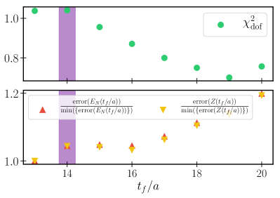
Figure 2: The top panel shows the correlated $\chi^{2}_{\mathrm{dof}}$ as a function of the final time slice $t_{f}/a$ for ensemble IV with $E_{N}(\vec{p}\,)=1.33\,\mathrm{GeV}$; the bottom panel shows the uncorrelated normalized statistical error of the fit parameters $E_{N}$ and $Z$. For the case shown we select the $t_{f}/a=14$ result.

IV.3 Three-point correlation functions

For the lattice calculations of three-point functions we use the sequential source method where we set the outgoing nucleon momentum $\vec{p}^{\,\prime}=\vec{0}$ for all our ensembles. We parametrize the data using Eqs. (20) and (23) with $E_{N}(\vec{p}^{\,\prime})$ = $m_{N}$. The initial energy $E_{N}(\vec{p}\,)$ is determined from the continuum dispersion relation (29). The momentum restriction, which we discussed in the previous section, translates to a range $0\leq Q^{2}<0.6\,\mathrm{GeV}^{2}$ for the three-point functions. With $Z(\vec{p}^{\,\prime})$ and $Z(\vec{p}\,)$ having been determined from the two-point correlation functions, the only free parameter left is $\mathcal{F}^{q}_{\Gamma}$. To achieve ground state dominance, one has to make sure that $aN_{T}\gg t^{\prime}\gg\tau\gg 0$ [cf. Eq. (20)]. We consider $\tau\in[\tau_{s},\tau_{e}]$ where $\tau_{s}$ is well above zero and $\tau_{e}$ well below $t^{\prime}$. The sink times vary with the ensemble (see the last column of Table 3). In Sec. IV.5 we examine possible excited state contaminations.

IV.4 Determination of the GFFs

As explained above, for every current $\Gamma=V$, $A$ or $T$, quark flavor $q$ and virtuality $-\mathsf{t}$, we need to solve the linear system Eq. (27), i.e., $\vec{\mathcal{F}}=M\cdot\vec{g}$, to extract the relevant form factors $\vec{g}$ from the vector of inequivalent matrix elements $\vec{\mathcal{F}}$ that correspond to nonvanishing rows of $M$. Here we drop all indices like the quark flavor $q$ and $\Gamma$ for convenience. In what follows $m$ denotes the number of independent form factors while $n\geq m$ is the length of $\vec{\mathcal{F}}$. Consequently, $M$ is a $n\times m$ matrix of maximal rank, i.e., $\operatorname{rank}(M)=m$.

The determination of the form factors is carried out in two ways. The first method consists of two steps: First we extract the ground state nucleon matrix elements $\mathcal{F}_{j}$ from the lattice three-point function data $c^{\tau}_{j}$, restricted to the range of insertion times $\tau\in[\tau_{s},\tau_{e}]$, through the numerical minimization of the $\chi^{2}$-function

$$\chi^{2}\big{(}\vec{\mathcal{F}}\,\big{)}=\sum\limits_{j=1}^{n}\sum\limits_{\tau,\tau^{\prime}=\tau_{s}}^{\tau_{e}}\delta c_{j}^{\tau}\left[\mathrm{cov}^{-1}_{j}\right]_{\tau\tau^{\prime}}\delta c_{j}^{\tau^{\prime}}\,,$$ (30)

where $\delta c_{j}^{\tau}$ is the difference

$$\delta c_{j}^{\tau}=c_{j}^{\tau}-\mathcal{F}_{j}\sqrt{Z(\vec{p}^{\,\prime})Z(\vec{p}\,)}\;\mathrm{e}^{-m_{N}(t^{\prime}-\tau)}\,\mathrm{e}^{-E_{N}(\vec{p}\,)\tau}$$ (31)

between the lattice data and the three-point function parametrization Eq. (23). The inverse covariance matrix $\mathrm{cov}_{j}^{-1}$ depends on the insertion times $\tau$ and $\tau^{\prime}$. One can easily generalize the fit to the situation of multiple source-sink distances $t^{\prime}$ if this is required or include excited state contributions. The index $j\in\{1,\ldots,n\}$ runs over all possible polarizations $\rho$ and initial momenta $\vec{p}$ (keeping the virtuality $Q^{2}$ fixed), which give nonvanishing contributions.

Once the fit parameters $\mathcal{F}_{j}$ are determined, one can minimize

$$\epsilon^{2}=\left(M\vec{g}-\vec{\mathcal{F}}\right)^{2}$$ (32)

to determine the form factors $\vec{g}$. The total number of parameters for this method is $m+n$ and, in particular for large virtualities, this number can be quite large (up to 50). This is not the only problem but it can happen that the resulting $\epsilon$ value is quite large and it is not clear how one should deal with such a situation.

Ideally, $\epsilon$ should be zero but this is only possible if $\vec{\mathcal{F}}$ is in the image of $M$ [cf. Eq. (32)]. Motivated by this observation, we carry out our fits employing a single step method, which combines the two subsequent steps into a single minimization problem, restricting the number of fit parameters to the relevant degrees of freedom. We start from the singular value decomposition,

$$M=U\cdot\Sigma\cdot V^{\intercal}$$ (33)

with orthogonal matrices $U\in\mathbb{R}^{n\times n}$, $V\in\mathbb{R}^{m\times m}$ and the matrix $\Sigma\in\mathbb{R}^{n\times m}$, which has nonvanishing entries only on the diagonal. The pseudoinverse $\Sigma^{+}$ is a $m\times n$ matrix that can easily be obtained, computing the inverses of the diagonal elements of $\Sigma$. Each vector $\vec{\mathcal{F}}$ within the image of $M$ can be uniquely expressed as a linear combination

$$\vec{\mathcal{F}}(\vec{\alpha}\,)=\sum\limits_{i=1}^{m}\alpha_{i}\,\vec{u}^{\,i}$$ (34)

of the first $m$ column vectors of $U$. Note that $m=\operatorname{rank}({M})$. Substituting $\vec{\mathcal{F}}\mapsto\vec{\mathcal{F}}(\vec{\alpha}\,)$ in Eq. (31) [and thereby Eq. (30)], we obtain a modified $\chi^{2}$-function that depends on the parameters $\alpha_{i}$, where $i\in\{1,\ldots,m\}$. Finally, we convert the extracted vector $\vec{\alpha}$ to the desired GFF vector,

$$\vec{g}=\left[V\Sigma^{+}U^{\intercal}\right]\sum\limits_{i=1}^{m}\alpha_{i}\,\vec{u}^{\,i}=\left[V\Sigma^{+}\right]\vec{\alpha}\,,$$ (35)

where in the last step $\Sigma^{+}$ is truncated to a $m\times m$ square matrix. In Fig. 3 we show for one example on the nearly physical quark mass ensemble VIII that this method works very well. In this case eight different lattice channels, listed in Table 4, are well described in terms of three fit parameters.

Table 4: Individual operator contributions to the fits shown in Fig. 3. The numbers in the legend of Fig. 3 correspond to the channels below. We parametrize the spatial lattice momentum $\vec{q}=\hat{k}2\pi/L$ in terms of $\hat{e}_{1}$,$\hat{e}_{2}$, and $\hat{e}_{3}$ which are unit vectors in the three spatial directions.

Channel	$\mathbb{P}^{\rho}$	$\mathcal{O}$	$\hat{k}$	Channel	#contrib.
0	$\mathbb{P}^{4}$	$\mathcal{O}_{1\,4}^{v_{2,a}}$	$\pm 2\hat{e}_{1}$	imaginary	2
		$\mathcal{O}_{2\,4}^{v_{2,a}}$	$\pm 2\hat{e}_{2}$		2
		$\mathcal{O}_{3\,4}^{v_{2,a}}$	$\pm 2\hat{e}_{3}$		2
1		$\mathcal{O}_{1}^{v_{2,b}}$	$\pm 2\hat{e}_{1}$	real	2
			$\pm 2\hat{e}_{2}$		2
2		$\mathcal{O}_{2}^{v_{2,b}}$	$\pm 2\hat{e}_{1}$	real	2
			$\pm 2\hat{e}_{2}$		2
3		$\mathcal{O}_{3}^{v_{2,b}}$	$\pm 2\hat{e}_{1}$	real	2
			$\pm 2\hat{e}_{2}$		2
4	$\mathbb{P}^{1}$	$\mathcal{O}_{2\,3}^{v_{2,a}}$	$\pm 2\hat{e}_{2}$, $\pm 2\hat{e}_{3}$	imaginary	4
	$\mathbb{P}^{2}$	$\mathcal{O}_{1\,3}^{v_{2,a}}$	$\pm 2\hat{e}_{1}$, $\pm 2\hat{e}_{3}$		4
	$\mathbb{P}^{3}$	$\mathcal{O}_{1\,2}^{v_{2,a}}$	$\pm 2\hat{e}_{1}$, $\pm 2\hat{e}_{2}$		4
5	$\mathbb{P}^{1}$	$\mathcal{O}_{3\,4}^{v_{2,a}}$	$\pm 2\hat{e}_{2}$	real	2
		$\mathcal{O}_{2\,4}^{v_{2,a}}$	$\pm 2\hat{e}_{3}$		2
	$\mathbb{P}^{2}$	$\mathcal{O}_{3\,4}^{v_{2,a}}$	$\pm 2\hat{e}_{1}$		2
		$\mathcal{O}_{1\,4}^{v_{2,a}}$	$\pm 2\hat{e}_{3}$		2
	$\mathbb{P}^{3}$	$\mathcal{O}_{2\,4}^{v_{2,a}}$	$\pm 2\hat{e}_{1}$		2
		$\mathcal{O}_{1\,4}^{v_{2,a}}$	$\pm 2\hat{e}_{2}$		2
6	$\mathbb{P}^{4}$	$\mathcal{O}_{1}^{v_{2,b}}$	$\pm 2\hat{e}_{3}$	real	2
7	$\mathbb{P}^{4}$	$\mathcal{O}_{2}^{v_{2,b}}$	$\pm 2\hat{e}_{3}$	real	2

A comparison of the two fit methods shows that the results are consistent within errors for all GFFs and for all ensembles. The single step method, however, results in somewhat smaller statistical errors and a smoother $Q^{2}$ dependence, especially for the induced GFFs. In Fig. 4 we directly compare the two methods. For the final results we only use the single step method. In Fig. 5 we show all $\chi^{2}_{\mathrm{dof}}$ values of all fits used in this paper to extract all considered GFFs: The correlated single step fits provide a very satisfactory description of the data.

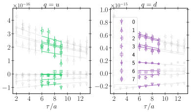
Figure 3: Fit results using the single step minimization method. We show ensemble VIII at the virtuality $Q^{2}=0.277\,\mathrm{GeV}^{2}$ in the vector channel. This corresponds to a spatial momentum transfer of $2\cdot 2\pi/L$, where we have averaged over all equivalent lattice directions. Three fit parameters $\vec{\alpha}=(\alpha_{1},\,\alpha_{2},\,\alpha_{3})^{\intercal}$ fully describe eight three-point functions. Colored points lie in the fit range $[\tau_{s},\tau_{e}]$ [cf. Eq. (30)]. On the left we show data for the $u$ quark and on the right for the $d$ quark (omitting disconnected contributions). The numbers in the legend refer to the channels listed in Table 4.

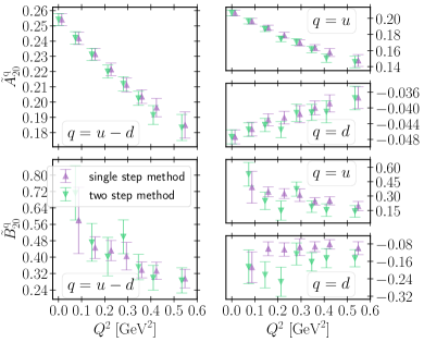
Figure 4: Comparison of single step and two step fit methods for the axial GFFs for ensemble VI. The right panels show $\widetilde{A}_{20}$ and $\widetilde{B}_{20}$ separately for the $u$ and $d$ quark (without disconnected contributions), the left panels for the isovector case.

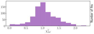
Figure 5: $\chi^{2}$ distribution of all GFF fits performed for this analysis.

IV.5 Excited states

For some of our ensembles we have three-point function data for different source-sink separations. This allows us to analyze the influence of excited states on the GFFs. Our analysis is based on ensemble IV with five source-sink separations in the range $t^{\prime}/a\in[7,17]$ and on ensemble VIII with three source-sink separations in the range $t^{\prime}/a\in[9,15]$. In physical units $t^{\prime}=15a$ corresponds to about $1\,\mathrm{fm}$. Ensemble VIII has data for eight values of $Q^{2}$ and this ensemble corresponds to an almost physical pion mass. We show results only for this ensemble, but our findings are consistent for both ensembles.

Figure 6: The vector GFFs vs $Q^{2}$ for different sink times $t^{\prime}$ for ensemble VIII.

For the tensor and axial GFFs we find that within statistical errors the $Q^{2}$ dependence is not affected by a variation of $t^{\prime}$. Only in the vector case, especially for $A_{20}^{u-d}$, excited state contaminations are visible (see Fig. 6). We have tried to parametrize these excited-state contributions to the three-point function with various multiexponential fit ansätze. This, however, introduces additional fit parameters, in particular the mass and the energy of the first excited state. The first excitation in the three-point function can be a multihadron state and hence its energy will in general not be well approximated by the single particle continuum dispersion relation. To parametrize excited state contributions clearly several source-sink separations are required. However, within present statistical errors little movement is visible for $t^{\prime}\gtrsim 0.9\,$fm, even in the $A_{20}$ channel where we achieve the highest accuracy; see Fig. 6 for an example. We therefore have restricted our GFF fits to ranges of $\tau$ where the data are well described by a single exponential (cf. Fig. 3). In all the cases $t^{\prime}$ is larger than 1 fm.

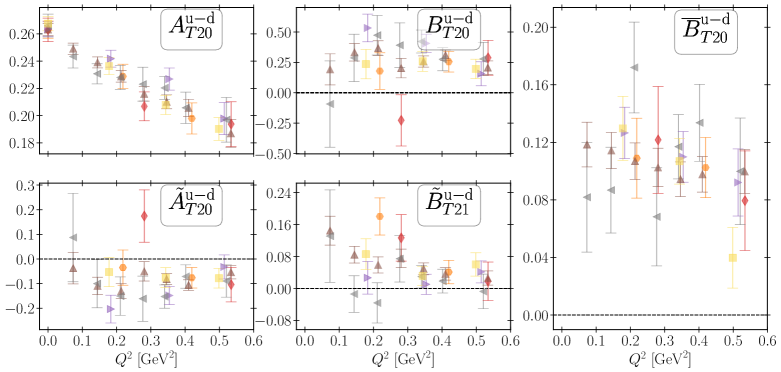
Figure 7: The vector and axial GFFs vs $Q^{2}$. Left: $A_{20}^{u-d}$, $B_{20}^{u-d}$ and $C_{20}^{u-d}$; right: $\widetilde{A}_{20}^{u-d}$ and $\widetilde{B}_{20}^{u-d}$. All results are for the isovector case and in the $\mathsf{\overline{MS}}$ scheme ($\mu=2\,\text{GeV}$).

Figure 8: The tensor GFFs $A^{u-d}_{T20}$, $B^{u-d}_{T20}$, $\widetilde{A}^{u-d}_{T20}$, $\widetilde{B}^{u-d}_{T21}$ and the linear combination $\overline{B}^{u-d}_{T20}$ in the $\mathsf{\overline{MS}}$ scheme ($\mu=2\,\text{GeV}$).

V Nucleon GFFs

Below we show results for the nucleon GFFs on a subset of the ensembles listed in Table 3. We restrict ourselves to $m_{\pi}<300\,$MeV and $m_{\pi}L>3.4$ and analyze the quark mass, volume and lattice spacing dependence. All results refer to the $\mathsf{\overline{MS}}$ scheme at $\mu=2\,\text{GeV}$.

V.1 Vector and axial GFFs

Results for the vector GFFs, $A_{20}^{u-d}$, $B_{20}^{u-d}$ and $C_{20}^{u-d}$, are shown in Fig. 8 (left) as a function of $Q^{2}=-\mathsf{t}$. We see that the discretization effects are negligible within errors (comparing ensembles I and XI, which give about the same pion mass and a similar value for $Lm_{\pi}$). Also the volume dependence (cf. V and VI) is small, although there is a slight trend towards larger values for $B_{20}^{u-d}$ if $Lm_{\pi}$ increases from about 4.2 to 6.7. For $A_{20}^{u-d}$ and $C_{20}^{u-d}$ we do not see any volume dependence within present errors. Similar statements hold for the quark mass dependence: For $A_{20}^{u-d}$ and $C_{20}^{u-d}$ it is negligible within errors, but for $B_{20}^{u-d}$ we see a trend towards lower values if the pion mass decreases down to 150 MeV (cf. VIII and VI). However, the latter could also be a volume artifact, since there is also a clear correlation between $Lm_{\pi}$ and $B_{20}^{u-d}$ (cf. ensembles VIII, V and VI where $Lm_{\pi}\simeq 3.5$, 4.2 and 6.7, respectively). $A_{20}^{u-d}$ and $B_{20}^{u-d}$ have a roughly linear $Q^{2}$ dependence for small $Q^{2}$, and $C_{20}^{u-d}$ is zero within errors. This agrees with the leading $\mathsf{t}$-dependence expected from covariant baryon chiral perturbation theory (BChPT, see below). We remark that also the individual (quark line connected) $u$ and $d$ quark contributions to $C_{20}^{u-d}$ are zero within error. So the smallness of this generalized form factor is not due to an approximate cancellation. For large $Q^{2}$ we expect that $A_{20}^{u-d}$ exhibits a dipolelike $Q^{2}$-dependence, which we saw in our former study (cf. Fig. 2 of Ref. Sternbeck et al. (2011)).

Results for the axial GFFs are shown in the right panel of Fig. 8. We see that a change of volume, quark mass or lattice spacing has almost no effect on the data. Within errors these effects cannot be resolved. Both form factors grow approximately linearly for $Q^{2}\to 0$. For $\widetilde{B}_{20}^{u-d}$ the statistical errors become larger for $Q^{2}\rightarrow 0$ whereas the errors for $\widetilde{A}_{20}^{u-d}$ are nearly independent of $Q^{2}$.

V.2 Tensor GFFs

Continuing with the tensor GFFs, we show results for $A^{u-d}_{T20}$, $B^{u-d}_{T20}$, $\widetilde{A}^{u-d}_{T20}$ and $\widetilde{B}^{u-d}_{T21}$ in Fig. 8. The dominant form factors are $A^{u-d}_{T20}$ and $B^{u-d}_{T20}$. For the available virtualities $A^{u-d}_{T20}$ rises linearly for $Q^{2}\to 0$, while $B^{u-d}_{T20}$ remains more or less constant, well above zero. Overall, the statistical errors for $A^{u-d}_{T20}$ are smaller than for $B^{u-d}_{T20}$. Volume, quark mass or lattice spacing effects cannot be resolved within errors.

The other two GFFs, $\widetilde{A}^{u-d}_{T20}$ and $\widetilde{B}^{u-d}_{T21}$, are smaller in comparison and, besides a few outliers, are best described by a constant. However, a final conclusion cannot be drawn as the statistical errors for both GFFs are rather large. We also study the linear combination

$$\overline{B}^{q}_{T20}=B^{q}_{T20}+2\widetilde{A}^{q}_{T20}\,,$$ (36)

which corresponds to the combination of GPDs $E_{T}+2\tilde{H}_{T}$ that is related to the Boer-Mulders function $h_{1}^{\perp}$ Boer and Mulders (1998). We find that the statistical error of $\overline{B}^{q}_{T20}$ is significantly smaller compared to the individual errors of $B^{q}_{T20}$ and $\widetilde{A}^{q}_{T20}$ (see Fig. 9). We will take advantage of this observation when looking at the transverse spin of the nucleon in Sec. VII. The results for $\overline{B}^{u-d}_{T20}$ are shown with the tensor GFFs in Fig. 8 for the same ensembles. The anticorrelations we find for $\overline{B}^{u-d}_{T20}$ are present for all ensembles.

Figure 9: Strong anticorrelations between $B^{q}_{T20}$ and $\widetilde{A}^{q}_{T20}$ for the example of ensemble VI.

VI Extraction of $\boldsymbol{J^{u-d}}$

The GFFs $A_{20}^{u-d}(\mathsf{t})$ and $B^{u-d}_{20}(\mathsf{t})$ are of particular interest since for $\mathsf{t}\to 0$ they are related to the total angular momentum Ji (1997)

$$J^{u-d}=\frac{1}{2}\left[A_{20}^{u-d}(0)+B_{20}^{u-d}(0)\right].$$ (37)

In order to estimate $J^{u-d}$ at the physical pion mass we analyze our data for $A_{20}^{u-d}(\mathsf{t})$ and $B^{u-d}_{20}(\mathsf{t})$, employing the BChPT formulas of Ref. Wein et al. (2014), which, however, we truncate at order $m_{\pi}^{3}$,

$$A^{u-d}_{20}(\mathsf{t},m_{\pi})=\left[1-\frac{(1+3\,g_{A}^{2})\,m_{\pi}^{2}\,\log(\frac{m_{\pi}^{2}}{\mu^{2}})}{16\,f_{\pi}^{2}\,\pi^{2}}\right]\,L\,$$

$$+\,m_{\pi}^{2}\,M_{2}^{A}\,+m_{\pi}^{3}\,M_{3}^{A}\,+\mathsf{t}(\,T_{0}^{A}+m_{\pi}^{2}\,T_{1}^{A})$$ (38)

and

$$B^{u-d}_{20}(\mathsf{t},m_{\pi})=\frac{g_{A}^{2}\,m_{\pi}^{2}\,\log(\frac{m_{\pi}^{2}}{\mu^{2}})}{16\,f_{\pi}^{2}\,\pi^{2}}L+\,\mathsf{t}(\,T_{0}^{B}+m_{\pi}^{2}\,T_{1}^{B})\,$$

$$+\left[1-\frac{(1+2\,g_{A}^{2})\,m_{\pi}^{2}\log(\frac{m_{\pi}^{2}}{\mu^{2}})}{16\,f_{\pi}^{2}\,\pi^{2}}\right]L^{B}\,+m_{\pi}^{2}\,M_{2}^{B}\,.$$ (39)

The fit parameters $T_{1}^{A}$ and $T_{1}^{B}$ are added since our data extend up to virtualities $-\mathsf{t}\approx(770\,\mathrm{MeV})^{2}\gg m_{\pi}^{2}$, however, these terms would naturally appear at the next order of BChPT. We determine the parameters $(L,M_{2}^{A},M_{3}^{A},T_{0}^{A},T_{1}^{A})$ and $(L,L^{B},M_{2}^{B},T_{0}^{B},T_{1}^{B})$ by carrying out combined fits to our data sets for $A^{u-d}_{20}(\mathsf{t},\,m_{\pi})$ and $B^{u-d}_{20}(\mathsf{t},\,m_{\pi})$. The remaining parameters in Eqs. (VI) and (VI) are constrained to $g_{A}=1.256$, $f_{\pi}=92.4\,\mathrm{MeV}$ and $\mu=1.0\,\mathrm{GeV}$.

Since it is not clear up to what values of $-\mathsf{t}$ and $m_{\pi}$ BChPT is applicable, we perform fits to all ensembles (set A) as well as fits using only ensembles with $m_{\pi}\leq 300\,\mathrm{MeV}$ (set B). In Fig. 10 we show the resulting fits for $\mathsf{t}=0$, where only in the case of $A_{20}^{u-d}$ we can directly compare to data points.

Figure 10: From top to bottom $A_{20}^{u-d}(0)$, $B_{20}^{u-d}(0)$ and $J^{u-d}$ as a function of the pion mass squared. The vertical solid line marks the physical pion mass; the vertical dashed line indicates our smallest pion mass. The A-band is from a fit of all our ensembles and the B-band from a fit where ensembles with $m_{\pi}>300\,\mathrm{MeV}$ are removed. For $A_{20}^{u-d}(0)$ we have lattice data which are shown in the top panel for comparison.

For set A the fit parameters have smaller statistical errors. For set B we see that $A_{20}^{u-d}$ increases with $m_{\pi}\rightarrow m_{\pi}^{\mathrm{phy}}$. For both sets we obtain values for $\chi_{\mathrm{dof}}^{2}$ of about 0.75, hence we cannot use the $\chi_{\mathrm{dof}}^{2}$ value to discriminate between the fit ranges. Instead, one may interpret the difference between fits A and B as a systematic uncertainty of the parameters. In Fig. 11 we show our fit for set A as a function of $Q^{2}$ at two fixed values of the pion masses ($m_{\pi}=422\,\text{MeV}$ and $150\,\text{MeV}$, ensembles III and VIII). Obviously, our ansatz for the $Q^{2}$ and $m_{\pi}^{2}$ dependence describes the lattice data well.

Again, we study the effect of the uncertainties of the renormalization constants using the strategy described in Appendix B.2. The final results are collected in Table 6, where we also quote the total angular momentum $J^{u-d}$. We refrain from extrapolating to $Q^{2}=0$ and $m_{\pi}=m_{\pi}^{\mathrm{phy}}$ in the other cases. Instead, in Table 6 we give the results for the form factors where no extrapolation in $Q^{2}$ is required, i.e. $A_{20}^{u-d}(0)$, $\widetilde{A}_{20}^{u-d}(0)$ and $A_{T20}^{u-d}(0)$, for our nearly physical point ensemble VIII. The moment $A_{20}^{u-d}(0)=\langle x\rangle_{u-d}$ agrees well with the results of the global fits to ensemble sets A and B and also the helicity and transversity moments $\widetilde{A}_{20}^{u-d}(0)=\langle x\rangle_{\Delta u-\Delta d}$ and $A_{T20}^{u-d}(0)=\langle x\rangle_{\delta u-\delta d}$ at the physical point ensemble are in agreement with the global data, see the top right panel of Fig. 8 and the top left panel of Fig. 8, respectively.

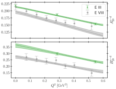
Figure 11: Chiral fit A versus $Q^{2}$ for two distinct pion masses: $m_{\pi}=422\,\text{MeV}$ (green) and $150\,\text{MeV}$ (grey). The corresponding data points (ensemble III and VIII) are shown as well.

Within the errors, our values agree with the isovector results of Ref. Alexandrou et al. (2017b).

Table 5: Results for $A_{20}^{u-d}(0,m_{\pi})$, $B_{20}^{u-d}(0,m_{\pi})$ and $J^{u-d}(m_{\pi})$, extrapolated to the physical pion mass $m_{\pi}^{\mathrm{phy}}$ using the ensemble sets A and B (see the text). The first error is statistical, the second error is due to the uncertainty of the renormalization constants.

Ensemble selection	A	B
$A_{20}^{u-d}(0,m_{\pi}^{\mathrm{phy}})$	$0.195\,(06)\,(03)$	$0.210\,(08)\,(04)$
$B_{20}^{u-d}(0,m_{\pi}^{\mathrm{phy}})$	$0.271\,(13)\,(03)$	$0.287\,(28)\,(04)$
$J^{u-d}(m_{\pi}^{\mathrm{phy}})$	$0.233\,(07)\,(03)$	$0.248\,(14)\,(04)$

Table 6: Results for $A_{20}^{u-d}$, $\widetilde{A}_{20}^{u-d}$ and $A_{T20}^{u-d}$ at the nearly physical pion mass $m_{\pi}=150\,\text{MeV}$ (ensemble VIII). The first error is statistical, the second error is due to the uncertainty of the renormalization constants.

Ensemble VIII	Value
$A_{20}^{u-d}(0,m_{\pi})$	$0.213\,(11)\,(04)$
$\widetilde{A}_{20}^{u-d}(0,m_{\pi})$	$0.240\,(07)\,(03)$
$A_{T20}^{u-d}(0,m_{\pi})$	$0.266\,(08)\,(04)$

VII Nucleon tomography

We use our lattice results for the vector GFFs $A_{20}(\mathsf{t})$, $B_{20}(\mathsf{t})$ and the linear combination $\overline{B}_{T20}(\mathsf{t})$ [cf. Eq. (36)] to investigate the transverse spin density of the nucleon. To this end, we transform these GFFs to the impact parameter space $G(\mathsf{t})\rightarrow G(\boldsymbol{b}_{\perp}^{2})$ with

$$G\left(\boldsymbol{b}_{\perp}^{2}\right)=\int\frac{\mathrm{d}^{2}\boldsymbol{\Delta_{\perp}}}{(2\pi)^{2}}\;e^{-i\boldsymbol{b_{\perp}}\cdot\boldsymbol{\Delta_{\perp}}}\>G\left(\mathsf{t}=-\boldsymbol{\Delta}^{2}_{\perp}\right)\,,$$ (40)

where we use the $p$-pole ansatz Diehl and Hägler (2005); Göckeler et al. (2007)

$$G(\mathsf{t})=\frac{G_{0}}{\left(1-\mathsf{t}/m_{p}^{2}\right)^{p}}$$ (41)

for the interpolation of our lattice results. The impact parameter $\boldsymbol{{b_{\perp}}}$ is defined in the transverse $x$-$y$ plane. It measures the transverse distance from the “center of momentum”

$$\boldsymbol{R}_{\perp}=\sum\limits_{i}\boldsymbol{r}_{i\,\perp}x_{i}\,,\quad\sum\limits_{i}x_{i}=1\,,$$ (42)

where $x_{i}$ is the momentum fraction of the $i$th parton Diehl and Hägler (2005); Soper (1977). We define

$$\boldsymbol{b}_{\perp}\coloneqq(b_{x},\,b_{y})\,,\quad\quad b_{\perp}\coloneqq\sqrt{\boldsymbol{b}_{\perp}^{2}}\,.$$ (43)

To compute the transverse spin density, we also have to evaluate the derivative of $G(b_{\perp}^{2})$ with respect to $b_{\perp}^{2}$,

$$G^{\prime}(b_{\perp}^{2})\coloneqq\frac{\partial}{\partial\,b_{\perp}^{2}}\,G(b_{\perp}^{2}).$$ (44)

The Fourier transform (40) of the $p$-pole ansatz (41) can be expressed in terms of the modified Bessel functions $K_{\nu}$ Diehl and Hägler (2005),

$$G(b_{\perp}^{2}) =\frac{G_{0}\,m_{p}^{2}\;(b_{\perp}m_{p})^{p-1}\,K_{p-1}(b_{\perp}m_{p})}{2^{p}\,\pi\,\Gamma(p)}\,.$$ (45)

The transverse spin density $\rho^{q}(x,\boldsymbol{{b_{\perp}}},\boldsymbol{s_{\perp}},\boldsymbol{S_{\perp}})$ describes the probability to find a quark with longitudinal momentum fraction $x$, flavor $q$ and transverse spin $\boldsymbol{s}_{\perp}$ at a distance $\boldsymbol{b}_{\perp}$ from the center of momentum of the nucleon with transverse spin $\boldsymbol{S}_{\perp}$. The explicit definition in terms of GPDs is given in Eq. (8) of Ref. Diehl and Hägler (2005). Here we consider the two transverse spin combinations,

$$\boldsymbol{s}_{\perp}=(1\,,0)\quad \text{and}\quad\boldsymbol{S}_{\perp}=(0\,,0)\,,$$ (46a)

$$\boldsymbol{s}_{\perp}=(0\,,0)\quad \text{and}\quad\boldsymbol{S}_{\perp}=(1\,,0)\,,$$ (46b)

where the first line describes a transversely polarized quark in an unpolarized nucleon and the second an unpolarized quark in a transversely polarized nucleon. In terms of GFFs the first moment of $\rho^{q}(x,\boldsymbol{{b_{\perp}}},\boldsymbol{s_{\perp}},\boldsymbol{S_{\perp}})$ for these spin combinations reads

$$\langle\rho\rangle^{q}(\boldsymbol{b_{\perp}},\boldsymbol{s_{\perp}},\boldsymbol{S_{\perp}}) =\int_{-1}^{1}\!\mathrm{d}x\,x\,\rho^{q}(x,\boldsymbol{{b_{\perp}}},\boldsymbol{s_{\perp}},\boldsymbol{S_{\perp}})$$

$$=\frac{1}{2}A_{20}^{q}(b_{\perp}^{2}) -\frac{\epsilon^{ij}\,b_{\perp}^{j}}{2m_{N}}\left(s_{\perp}^{i}\overline{B}_{T20}^{q\,\prime}(b_{\perp}^{2})+S_{\perp}^{i}B_{20}^{q\,\prime}(b_{\perp}^{2})\right)\,.$$ (47)

For arbitrary spins $\boldsymbol{S}_{\perp}$ and $\boldsymbol{s}_{\perp}$ Eq. (47) will contain additional terms and we refer the reader to Refs. Diehl and Hägler (2005); Göckeler et al. (2007).

Figure 12: The pole mass $m_{p}$ and $\chi^{2}_{\mathrm{dof}}$ as a function of the fixed parameter $p$ for ensemble VI. The colored lines correspond to fits to $A_{20}^{q}$, $B_{20}^{q}$ and $\overline{B}_{T20}^{q}$ from top to bottom and flavor $q$ from left to right.

Figure 13: The $p$-dependence of the transverse spin density for a transversely polarized $d$-quark in an unpolarized nucleon. The yellow cross indicates the maximum of the density. The black contour lines are drawn equidistantly with a difference of 0.05.

We fit the GFFs for ensemble VI to the $p$-pole ansatz Eq. (41). Due to the limited number of data points at our disposal, where we restricted ourselves to the kinematic range $-\mathsf{t}\leq 0.6\,\mathrm{GeV}^{2}$, we find it impossible to simultaneously determine all three fit parameters, $p$, $m_{p}$ and $G_{0}$. In particular the exponent $p$ is strongly correlated with the pole mass $m_{p}$. This is demonstrated in Fig. 12: An increase of $p$ results in a larger value of $m_{p}$, whereas $\chi^{2}_{\mathrm{dof}}$ does not significantly change. Therefore, we cannot constrain $p$.

This arbitrariness means it is difficult to obtain reliable, parametrization independent results for the moment $\langle\rho\rangle^{q}(\boldsymbol{b_{\perp}},\boldsymbol{s_{\perp}},\boldsymbol{S_{\perp}})$ as a function of $\boldsymbol{b_{\perp}}$. This distribution has been studied in the past (see, e.g., Göckeler et al. (2007)), but we find that its shape strongly depends on the value of $p$. In Fig. 13 we show $\langle\rho\rangle^{q}(\boldsymbol{b_{\perp}},\boldsymbol{s_{\perp}},\boldsymbol{S_{\perp}})$ for $\boldsymbol{s}_{\perp}=(1,0)$ and $\boldsymbol{S}_{\perp}=(0,0)$ for four distinct values of $p$ ranging from 1.45 up to 3.0. We see that with increasing $p$ the density becomes less localized in the impact parameter plane and the maximum of the density is shifted away from the center. This also holds for other spin combinations.

Table 7: The half $\boldsymbol{b_{\perp}}$-integrated moments for $p=2$, also shown in Fig. 15. The errors are statistical. The systematic error of the $p$-dependence is about 0.02.

	$\boldsymbol{s}_{\perp}=(1\,,0)$	$\boldsymbol{s}_{\perp}=(0\,,0)$
	$\boldsymbol{S}_{\perp}=(0\,,0)$	$\boldsymbol{S}_{\perp}=(1\,,0)$
$\langle\rho\rangle^{u}_{-}$	0.312 (26)	0.403 (12)
$\langle\rho\rangle^{u}_{+}$	0.688 (26)	0.597 (12)
$\langle\rho\rangle^{d}_{-}$	0.262 (27)	0.666 (17)
$\langle\rho\rangle^{d}_{+}$	0.738 (27)	0.334 (17)

We discovered that some integrated quantities have a much milder $p$-dependence, namely the half $\boldsymbol{b_{\perp}}$-integrated moments

$$\langle\rho\rangle^{q}_{+}(\boldsymbol{s_{\perp}},\boldsymbol{S_{\perp}}) =\frac{1}{Z_{\rho}}\int\limits_{-\infty}^{+\infty}\!\mathrm{d}b_{x}\!\!\int\limits_{0}^{+\infty}\!\mathrm{d}b_{y}\,\langle\rho\rangle^{q}(\boldsymbol{b_{\perp}},\boldsymbol{s_{\perp}},\boldsymbol{S_{\perp}})\,,$$ (48a)

$$\langle\rho\rangle^{q}_{-}(\boldsymbol{s_{\perp}},\boldsymbol{S_{\perp}}) =\frac{1}{Z_{\rho}}\int\limits_{-\infty}^{+\infty}\!\mathrm{d}b_{x}\!\!\int\limits_{-\infty}^{0}\!\mathrm{d}b_{y}\,\langle\rho\rangle^{q}(\boldsymbol{b_{\perp}},\boldsymbol{s_{\perp}},\boldsymbol{S_{\perp}})\,,$$ (48b)

with the normalization factor

$${Z_{\rho}} =\int\limits_{-\infty}^{+\infty}\!\mathrm{d}b_{x}\,\int\limits_{-\infty}^{+\infty}\!\mathrm{d}b_{y}\,\langle\rho\rangle^{q}(\boldsymbol{b_{\perp}},\boldsymbol{s_{\perp}},\boldsymbol{S_{\perp}})\,.$$ (49)

The integrated moment $\langle\rho\rangle^{q}_{+}(\boldsymbol{s_{\perp}},\boldsymbol{S_{\perp}})$ is the probability, weighted with the longitudinal momentum fraction $x$, to find a quark with flavor $q$ in the upper part ($b_{y}\geq 0$) of the impact parameter space and $\langle\rho\rangle^{q}_{-}(\boldsymbol{s_{\perp}},\boldsymbol{S_{\perp}})$ is the $x$-weighted probability to find a quark with flavor $q$ in the lower part ($b_{y}\leq 0$). These integrated moments are a measure for the asymmetry of the transverse spin density. They depend much less on the value of $p$ than $\langle\rho\rangle^{q}(\boldsymbol{b_{\perp}},\boldsymbol{s_{\perp}},\boldsymbol{S_{\perp}})$ does. This is demonstrated in Fig. 14, where $\langle\rho\rangle^{d}_{+}$ and $\langle\rho\rangle^{d}_{-}$ are shown as functions of $p$ for the transverse spin combination in Eq. (46a). Doubling $p$, both integrated moments change by only 5% and 15%, respectively. We find this mild $p$-dependence for all considered transverse spin and flavor combinations and consider these integrated moments as the better candidates for reliable lattice estimates. Our results for $\langle\rho\rangle^{q}_{\pm}$ for up and down quark for our two transverse spin combinations [Eq. (46)] are shown in Fig. 15. The errors shown are statistical only. The figure corresponds to the power $p=2$, and one may add systematic errors of about 0.02 due to the $p$-dependence; see Fig. 14. The numerical values are listed in Table 7.

We see the probability of a transversely polarized $u$- or $d$-quark in an unpolarized nucleon is higher ($\sim 70\%$) in the $b_{y}>0$ part of the impact parameter space than in the $b_{y}<0$ part ($\sim 30\%$). For a transversely polarized nucleon however the probabilities of an unpolarized $u$- or $d$-quark differ: The unpolarized $d$-quark is more likely in the $b_{y}<0$ part ($67\%$), while a $u$-quark is more likely in the $b_{y}>0$ part (60%) of the impact parameter space.

Figure 14: Dependence of $\langle\rho\rangle^{d}_{+}\left(\boldsymbol{s_{\perp}},\boldsymbol{S_{\perp}}\right)$ and $\langle\rho\rangle^{d}_{-}\left(\boldsymbol{s_{\perp}},\boldsymbol{S_{\perp}}\right)$ on the power $p$ of the pole ansatz. The combination of transverse spins is $\boldsymbol{s_{\perp}}=(1,0)$ and $\boldsymbol{S_{\perp}}=(0,0)$. The errors are statistical only. The systematics due to the uncertainty of the power $p$ amount to about 0.02.

Figure 15: Probability (weighted with $x$) to find a $u$- or $d$-quark in the upper/ lower part ($b_{y}\lessgtr 0$) of the impact parameter space; left for a transversely polarized quark in an unpolarized nucleon; right for an unpolarized quark in a transversely polarized nucleon.

VIII Summary

We have calculated all quark GFFs, corresponding to operators with one derivative, of the nucleon GPDs at leading twist-2. Our lattice calculation includes the dominating connected contributions and neglects contributions from disconnected diagrams. The available gauge ensembles cover a wide range of quark masses and volumes. However, the three available lattice spacings only vary from 0.081 fm down to 0.060 fm. Within errors, all GFFs show a mild dependence on the quark mass, lattice spacing and volume.

We have compared two different fitting strategies for the GFFs and found that the direct fit method appears to be more reliable. With this method the number of fit parameters is reduced to the relevant degrees of freedom. We recommend to use this method in future studies. The final results for the GFFs are shown in Figs. 8 and 8.

We have also studied the total angular momentum and the transverse spin density of quarks in the nucleon. Both quantities can be extracted from fits to our GFF data. For the total angular momentum we obtain a similar estimate in the isovector case as ETMC in Ref. Alexandrou et al. (2017b). Contributions from disconnected diagrams are not included in our lattice calculation. From Ref. Alexandrou et al. (2017b) we know that these are small. Nevertheless, in the isoscalar case they should definitely be taken into account. For the second moment of the transverse spin density we have found that its distribution in impact parameter space strongly depends on the $\mathsf{t}$-dependence of the GFF data. The shape of the distribution depends on the value of $p$ that is used within a $p$-pole ansatz. High precision data at small and large values of $-\mathsf{t}$ would be required to eliminate this ambiguity. For integrated moments this situation improves. In Fig. 15 we provide lattice estimates for the $x$-weighted probabilities of a transversely polarized (unpolarized) light quark in the upper or lower part of the impact parameter space, within an unpolarized (transversely polarized) nucleon. Contributions from higher moments are not yet available but constitute an interesting object for future study.

Appendix A Operator multiplets for the tensor GFFs

In this study we use 16 linear combinations of operators for the tensor GFFs. The first eight from the $h_{1,a}$ multiplet read

$$\mathcal{O}_{1}^{h_{1,a}} =\sqrt{\frac{2}{3}}(\mathcal{O}_{132}^{\intercal}+\frac{1}{2}\mathcal{O}_{123}^{\intercal}+\frac{1}{2}\mathcal{O}_{231}^{\intercal}),$$

$$\mathcal{O}_{2}^{h_{1,a}} =\sqrt{\frac{2}{3}}(\mathcal{O}_{142}^{\intercal}+\frac{1}{2}\mathcal{O}_{124}^{\intercal}+\frac{1}{2}\mathcal{O}_{241}^{\intercal}),$$

$$\mathcal{O}_{3}^{h_{1,a}} =\sqrt{\frac{2}{3}}(\mathcal{O}_{143}^{\intercal}+\frac{1}{2}\mathcal{O}_{134}^{\intercal}+\frac{1}{2}\mathcal{O}_{341}^{\intercal}),$$

$$\mathcal{O}_{4}^{h_{1,a}} =\sqrt{\frac{2}{3}}(\mathcal{O}_{243}^{\intercal}+\frac{1}{2}\mathcal{O}_{234}^{\intercal}+\frac{1}{2}\mathcal{O}_{342}^{\intercal}),$$

$$\mathcal{O}_{5}^{h_{1,a}} =\sqrt{2}\mathcal{O}_{2\{13\}}^{\intercal},$$

$$\mathcal{O}_{6}^{h_{1,a}} =\sqrt{2}\mathcal{O}_{2\{14\}}^{\intercal},$$

$$\mathcal{O}_{7}^{h_{1,a}} =\sqrt{2}\mathcal{O}_{3\{14\}}^{\intercal},$$

$$\mathcal{O}_{8}^{h_{1,a}} =\sqrt{2}\mathcal{O}_{3\{24\}}^{\intercal}\,.$$

The remaining eight make up the $h_{1,b}$ multiplet and read

$$\mathcal{O}_{9}^{h_{1,b}} =\sqrt{\frac{1}{2}}(\mathcal{O}_{122}^{\intercal}-\mathcal{O}_{133}^{\intercal}),$$

$$\mathcal{O}_{10}^{h_{1,b}} =\sqrt{\frac{1}{2}}(\mathcal{O}_{211}^{\intercal}-\mathcal{O}_{233}^{\intercal}),$$

$$\mathcal{O}_{11}^{h_{1,b}} =\sqrt{\frac{1}{2}}(\mathcal{O}_{311}^{\intercal}-\mathcal{O}_{322}^{\intercal}),$$

$$\mathcal{O}_{12}^{h_{1,b}} =\sqrt{\frac{1}{2}}(\mathcal{O}_{411}^{\intercal}-\mathcal{O}_{422}^{\intercal}),$$

$$\mathcal{O}_{13}^{h_{1,b}} =\sqrt{\frac{1}{6}}(\mathcal{O}_{122}^{\intercal}+\mathcal{O}_{133}^{\intercal}-2\mathcal{O}_{144}^{\intercal}),$$

$$\mathcal{O}_{14}^{h_{1,b}} =\sqrt{\frac{1}{6}}(\mathcal{O}_{211}^{\intercal}+\mathcal{O}_{233}^{\intercal}-2\mathcal{O}_{244}^{\intercal}),$$

$$\mathcal{O}_{15}^{h_{1,b}} =\sqrt{\frac{1}{6}}(\mathcal{O}_{311}^{\intercal}+\mathcal{O}_{322}^{\intercal}-2\mathcal{O}_{344}^{\intercal}),$$

$$\mathcal{O}_{16}^{h_{1,b}} =\sqrt{\frac{1}{6}}(\mathcal{O}_{411}^{\intercal}+\mathcal{O}_{422}^{\intercal}-2\mathcal{O}_{433}^{\intercal}).$$

Appendix B Renormalization procedure

The renormalization factors are products of perturbative and nonperturbative parts:

$$Z^{\mathsf{\overline{MS}}}_{\mathcal{O}}\coloneqq Z_{\mathcal{O},\mathsf{RI^{\prime}}}^{\mathsf{\overline{MS}}}Z_{\mathcal{O},\mathrm{bare}}^{\mathsf{RI^{\prime}}}\,.$$ (50)

The nonperturbative factor $Z^{\mathsf{RI^{\prime}}}_{\mathcal{O},\mathrm{bare}}$ translates the bare lattice data to the regularization scheme independent momentum subtraction ($\mathsf{RI^{\prime}\textnormal{-}MOM}$) scheme Martinelli et al. (1995); Chetyrkin and Retey (2000), while the perturbative factor $Z_{\mathcal{O},\mathsf{RI^{\prime}}}^{\mathsf{\overline{MS}}}$ matches from the $\mathsf{RI^{\prime}\textnormal{-}MOM}$ to the $\mathsf{\overline{MS}}$ scheme. This is calculated in continuum perturbation theory and is known for our operator multiplets to three-loop accuracy Gracey (2003).

B.1 Nonperturbative renormalization

The nonperturbative renormalization factors $Z^{\mathsf{RI^{\prime}}}_{\mathcal{O},\mathrm{bare}}$ are extracted as follows. In a first step we gauge-fix a subset of our gauge configurations to Landau gauge and calculate (in momentum space) the quark propagator

$$S_{\alpha\beta}(a,p)=\frac{a^{8}}{V}\sum_{xy}e^{-ip\cdot(x-y)}\left\langle q_{\alpha}(x)\bar{q}_{\beta}(y)\right\rangle$$ (51)

(color indices are suppressed) and the three-point functions

$$G^{{j,\mu}}_{\alpha\beta}(a,p)=\frac{a^{12}}{V}\sum_{xyz}e^{-ip\cdot(x-y)}\left\langle q_{\alpha}(x)\,\mathcal{J}^{j}_{\mu}(z)\,\bar{q}_{\beta}(y)\right\rangle$$ (52)

with $\mathcal{J}^{j}_{\mu}(z)\coloneqq\bar{q}(z)\,\mathsf{\Gamma}^{j}\overleftrightarrow{\nabla}_{\!\mu}q(z)=\bar{q}(z)\mathcal{O}^{j}_{\mu}(z)q(z)$. $\mathsf{\Gamma}^{j}$ denotes one of the sixteen possible products of Euclidean gamma matrices, $\gamma^{n_{1}}_{1}\cdots\gamma_{4}^{n_{4}}$ ($n_{\mu}\in\{0,1\}$), and the covariant lattice derivative acts on the respective left or right quark propagators resulting from the integration over the quark fields.

Next the vertex function $\Gamma_{\mathcal{O}}$ is constructed for each operator $\mathcal{O}(0)$ by combining the appropriate $G^{j,\mu}$s and amputating the fermion legs,

$$\Gamma_{\mathcal{O}}(a,p)\coloneqq S^{-1}(a,p)G_{\mathcal{O}}(a,p)S^{-1}(a,p)\,.$$ (53)

The renormalized vertex reads

$$\Gamma^{R}_{\mathcal{O}}(p,\mu^{2})=\frac{Z^{\mathsf{RI^{\prime}}}_{\mathcal{O},\mathrm{bare}}(a,\mu^{2})}{Z_{q}(a,\mu^{2})}\Gamma_{\mathcal{O}}(a,p)\,,$$ (54)

where the $\mathsf{RI^{\prime}\textnormal{-}MOM}$ renormalization condition

$$\left.\frac{1}{12}\operatorname{Tr}\left(\Gamma^{R}_{\mathcal{O}}\left[\Gamma^{(0)}_{\mathcal{O}}\right]^{-1}\right)\stackrel{{\scriptstyle!}}{{=}}1\quad\right|_{p^{2}=\mu^{2}}$$ (55)

is imposed in the chiral limit. The quark wave function renormalization factor is given by

$$Z_{q}(a,\mu^{2})=\left.\frac{-i\operatorname{Tr}\left(\gamma_{\lambda}\bar{p}_{\lambda}\,S^{-1}(a,p)\right)}{12\bar{p}^{2}}\right|_{p^{2}=\mu^{2}}$$ (56)

after extrapolation to the massless limit. In Eq. (56) we employ the lattice tree-level expression for the massless quark propagator; i.e., we set $a\bar{p}_{\lambda}\coloneqq\sin(ap_{\lambda})$. Similarly we use the lattice tree-level expression for the Born term $\Gamma^{(0)}_{\mathcal{O}}$ to reduce lattice discretization effects. For the example of the operator $\mathcal{O}^{\mu\nu}_{V,q}$ this reads

$$\Gamma^{(0)}_{\mathcal{O}}(p)=i\left(\gamma_{\mu}\bar{p}_{\nu}+\gamma_{\nu}\bar{p}_{\mu}\right)\,.$$ (57)

B.2 Propagation of renormalization constant errors

Our estimates for the renormalization factors carry an uncertainty which has to be propagated into the GFFs. We do this in a very naive but conservative way by carrying out the whole analysis both using the central values of the renormalization factors and adding the error of these factors to their central values. The difference between these two sets of results is then due to the uncertainty of the renormalization. This procedure is applied to all ensembles and to all the available virtualities $Q^{2}$. We find that the relative error is almost independent of $Q^{2}$ and the considered ensemble. Hence, for each GFF we decided to take the largest value of this uncertainty as an estimator of the error. These relative uncertainties are shown in Table 2.