Non-locality effect on the entanglement entropy in deSitter

Abstract

We investigate the effect of infrared non-locality on the entanglement between two causally separated open-charts in the deSitter space-time. Inspired by the work of Maldacena and Pimentel who gave a precise methodology for the computation of the long-range entanglement for the local massive scalar field theory on deSitter space-time, we aim to investigate the change in behaviour of this long-range entanglement due to the presence of infrared non-locality in the theory. By considering a non-local scalar field theory where the non-locality becomes important in the infrared, we follow the footsteps of Maldacena and Pimentel to compute the entanglement entropy of the free non-local scalar field theory in the Bunch-Davies vacuum. It is found that the presence of infrared non-locality will have strong effect on the long-range entanglement. In some case it is noted that if the strength of non-locality is large then it will tend to decrease the long-range entanglement in the infrared. We also consider the behaviour of Rényi entropy, where a strong role of non-locality on the entropy is noticed.

1 Introduction

Entanglement entropy offers a very valuable insight in to the study of long-range quantum phenomenon which occurs in condensed matter system (see [1, 2] and the references therein). This powerful concept also allows one to investigate the nature of long-range correlations in the field theories, as it gives a way to understand the behaviour of correlation between different localised subsystems of a quantum system. Local quantum field theory is a well established framework where meaningful computation can be performed. Moreover, in local QFTs which are ultraviolet finite it is known that the entanglement entropy follows area law [3, 4]. However, not much is known about the situation in the case when non-locality is present in the system. Non-locality is indeed intriguing in the sense the effect it can have on the long-range entanglement. Recently in [5] a first attempt has been made to investigate the effect of infrared non-locality on the behaviour of entanglement entropy in anti-deSitter space-time.

Non-locality is a very crucial feature of quantum field theories which arises naturally at low-energies due to the running of couplings because of quantum corrections. For example in quantum theory if the coupling has energy dependence $g(\mu)$ (where $\mu$ is the running energy scale), then such running can be incorporated in the action by generalising the coupling $g(\mu)\to g(-\Box)$, where $\Box$ is the square of covariant derivative. This offers a non-local infrared modifications of the field theory. In fact such kind of non-local modification has been extensively studied in [6], with the aim of obtaining an infrared non-local modification to gravity. Such infrared modification of gravity has recently been a subject of great interest due to its ability in generating a late time cosmic acceleration mimicking dark energy [7, 8, 9]. Universe undergoing an accelerated expansion can be beautifully represented as a deSitter space-time, thereby putting a strong emphasis on the importance of studying the field theory on deSitter space-time.

Recently, studies on non-local theory have gained momentum in regard to ultraviolet modification of various QFTs where it is seen that such non-local modifications offer a well-behaved UV finite theory which can be super-renormalizable [10, 11, 12, 13, 14]. Such UV modification of theory by an addition of non-locality provides an extra suppression factor in the propagator of theories at high-energies thereby rendering the theory well-behaved in UV. Non-local theories have also been investigated in relation to black-hole information loss paradox [15, 16]. Our aim in this paper is to investigate the infrared low-energy effects of non-local modifications of theory. We wish to do this by investigating the entanglement between the two causally dis-connected charts of deSitter space-time. In cosmological scenarios we expect that entanglement could exists beyond the Hubble horizon as deSitter expansion will eventually rips off a pair of particle which were created within the causally connected region (inside Hubble radius). If the system has non-locality (which is generated by some mechanism) and it becomes dominant in infrared, then such non-locality will very-likely affect the entanglement of the two causally disconnected regions of deSitter space. It is our aim to study this effect of non-locality on the entanglement between two causally disconnected regions of deSitter.

In the paper we consider a non-local scalar field theory which resides on a fixed space-time (deSitter space-time for this paper). Here the non-locality arises once one of the field is integrated out from the coupled system of local theory. The residual action describes the behaviour of the massive non-local scalar field. This non-local theory has recently been investigated in various contexts [17, 18, 5]. The purpose is to understand the effect of such infrared non-locality on the low-energy physics. Interestingly it is seen in [18] (see the references therein for the IR problem of the dS propagator) that the presence of the non-locality offers a well-behaved infrared finite deSitter propagator of the scalar field theory which decays at large time scale. DeSitter propagator of massless local scalar field has been a long standing problem where the propagator gets IR divergences and the massless limit of massive propagator is not well-defined. It was found in [18] that the presence of non-locality helps in overcoming these issues very elegantly thereby advocating the importance of non-local effects in the IR physics. Motivated by this we then investigated the effect of such non-locality on the behaviour of entanglement entropy on AdS [5] where the universal finite part was seen to have a characteristic oscillating feature due to the presence of non-locality.

These studies pushed us further to explore the effect this infrared non-locality will have on the entanglement between two causally disconnected regions of deSitter space-time which is the work presented in this paper. In [19] the authors investigated the nature of the long-range entanglement entropy on deSitter space-time, which they found it to be absent in flat space-time and is only specific to deSitter space-time. They described an elegant way to specifically extract the part of entanglement entropy which captures information about the long-range entanglement. We follow the same footsteps described in [19] to investigate whether the non-locality can play a significant role in affecting the long-range entanglement. As scalar fields play an important role in cosmology in understanding both early and late-time universe, it is therefore important to investigate the effect non-localities (which could have arisen either because of quantum effects or due to some other mechanism) will have on the long-range entanglement.

The paper is organised as follows. In section 2 we consider the toy model for the non-local theory. In section 3 we give a setup of the computation of the entanglement entropy in dS. in section 4 we compute the modes of the non-local scalar field on deSitter. In section 5 we compute the density matrix for our theory and correspondingly compute the entanglement entropy. We compute the Rényi entropy and entanglement negativity for our non-local system in section 6. We conclude the paper with a summary of results and discussion in section 7.

2 Non-local scalar field

In this section we consider a scalar field theory which leads to non-local action when one of the scalar gets decoupled from system. Consider the following action,

$$S=\int{\rm d}x\sqrt{-g}\biggl{[}\frac{1}{2}(\partial\phi)^{2}+\frac{1}{2}(\partial\chi)^{2}+\frac{m^{2}}{2}\phi^{2}-\lambda\phi\chi\biggr{]}\,,$$ (2.1)

where $\phi$ and $\chi$ are two scalar fields on curved non-dynamical background, $\lambda$ is their interaction strength and $m$ is mass of scalar $\phi$. The equation of motion of two fields give $(-\Box+m^{2})\phi-\lambda\chi=0$ and $-\Box\chi-\lambda\phi=0$. Integrating out $\chi$ from the second equation of motion yields $\chi=\lambda(-\Box)^{-1}\phi$. This when plugged back into the action (2.1) yields a massive non-local theory for scalar $\phi$ whose action is given by,

$$S_{NL}=\int{\rm d}x\sqrt{-g}\biggl{[}\frac{1}{2}(\partial\phi)^{2}+\frac{m^{2}}{2}\phi^{2}-\frac{\lambda^{2}}{2}\phi\frac{1}{-\Box}\phi\biggr{]}\,.$$ (2.2)

This non-local action has issues of tachyon. In simple case of flat space-time it is noticed that the non-local piece in action reduces to $\phi(-p)(-\lambda^{2}/p^{2})\phi(p)$ (where $\phi(p)$ is the fourier transform of field $\phi(x)$). This piece correspond to something like tachyonic mass indicating instability of vacuum. Also, in massless case if we write

$$\phi_{-}=(\phi+\chi)/\sqrt{2}\,,\hskip 14.22636pt\phi_{+}=(\phi-\chi)/\sqrt{2}\,,$$ (2.3)

then the local action in eq. (2.1) can be reduced to action of two decoupled free scalar fields $\phi_{-}$ and $\phi_{+}$ of mass-square $-\lambda$ and $\lambda$ respectively.

$$S_{\rm FT}=\int{\rm d}x\sqrt{-g}\biggl{[}\frac{1}{2}(\partial\phi_{-})^{2}+\frac{1}{2}(\partial\phi_{+})^{2}-\frac{\lambda}{2}\phi_{-}^{2}+\frac{\lambda}{2}\phi_{+}^{2}\biggr{]}\,.$$ (2.4)

Immediately we notice the field $\phi_{-}$ is tachyonic. If we change the sign of $\lambda$ then $\phi_{+}$ becomes tachyonic. This tachyonic issue only disappears for case when $\lambda=0$ which correspond to two uncoupled massless scalar fields. In the massive case things are just more involved, but tachyonic issue remains. To see this more clearly we make a linear transformation by writing the original set of field ($\phi$ and $\chi$) in terms of new fields ($\phi_{1}$ and $\phi_{2}$) as

$$\phi=A_{1}\phi_{1}+A_{2}\phi_{2}\,,\hskip 14.22636pt\chi=B_{1}\phi_{1}+B_{2}\phi_{2}\,.$$ (2.5)

By demanding that the transformed Lagrangian is a decoupled system of two scalars we get the constraints

$$A_{1}A_{2}+B_{1}B_{2}=0\,,\hskip 14.22636ptm^{2}A_{1}A_{2}-\lambda A_{1}B_{2}-\lambda A_{2}B_{1}=0\,.$$ (2.6)

By expressing $A_{1}=\kappa B_{1}$ and $B_{2}=-\kappa A_{2}$, one can express the transformed lagrangian in terms of $\kappa$, $A_{2}$ and $B_{1}$. The parameters $B_{1}$ and $A_{2}$ can be determined by requiring to be nonzero and the kinetic terms for the transformed fields to be in canonical form. This gives a condition on the parameter $\kappa$ to be

$$\lambda\kappa^{2}+m^{2}\kappa-\lambda=0\,,$$ (2.7)

and the transformed lagrangian to be

$$S_{\rm FT}=\int{\rm d}x\sqrt{-g}\biggl{[}\frac{1}{2}(\partial\phi_{1})^{2}+\frac{1}{2}(\partial\phi_{2})^{2}-\frac{1}{2}\lambda\kappa\phi_{1}^{2}+\frac{\lambda}{2\kappa}\phi_{2}^{2}\biggr{]}\,,$$ (2.8)

where $\kappa$ is determined from the equation (2.7). If $\kappa_{1}$ and $\kappa_{2}$ are two roots of the eq. (2.7), then they satisfy the relation $\kappa_{1}\kappa_{2}=-1$. This will mean that one of the transformed field will be tachyonic in nature. So the tachyonic issue is inherent to the kind of non-local system considered here.

Such tachyonic problem can be avoided if we consider $\lambda^{2}\to-\lambda^{2}$. In this situations the poles of the theory are however complex in nature. In particular, when one considers massless theory where transformation as in eq. (2.3) can be applied, it is found that decoupled action for two scalar fields $\phi_{-}$ and $\phi_{+}$ have mass-square $-i\lambda$ and $i\lambda$ respectively. This results in complex mass-poles. Field theory with complex poles have been a well studied subject since the $60$’s [20, 21, 22, 23], where unitarity, causality of such theories have been investigated. In light of those works one can therefore safely have trust in the exploration of such non-local theories and consider them as an effective infrared theory which has a one particular kind of non-locality.

3 Setup for Entanglement Entropy on dS

In this section we study the entanglement entropy for the above non-local quantum field theory on deSitter space-time. We choose the standard vacuum-state [24, 25, 26] (which is commonly referred to as Euclidean/Bunch-Davies vacuum) for the field theory described on non-dynamical background deSitter space-time.

As described in [19], we consider a spherical surface which divides the dS space-time into interior and exterior regions. The entanglement between the modes lying on the two sides of the surface is computed by tracing out the modes lying on the exterior. We consider the size of sphere to be much larger than the deSitter radius, $R\gg R_{\rm dS}=H^{-1}$, where $H$ is the Hubble’s constant. The entanglement entropy is computed using the usual methods and as expected the UV singularity comes from local physics (having no effect from non-locality) which we ignore. For very large spheres in four space-time dimensions, the finite piece has a term that goes as logarithm of the area of surface, we will focus on the coefficient of this piece. In odd-dimensions there are contribution to finite term which goes like area and a constant term. In odd-dimensions we therefore focus on the constant term.

We compute the entanglement entropy for the non-local scalar field. To achieve this, we need to compute the density matrix by tracing out from modes lying outside the surface. When this spherical surface is taken all the way to the deSitter boundary then it is seen that the problem has a $SO(1,3)$ symmetry. The presence of this symmetry offers a helping hand in the computation of the density matrix and the entanglement entropy associated to it. The successful computation of the density matrix allows us to compute even Renyi entropies.

We follow [27] in defining entanglement entropy. In a space-time divided in two regions by a closed surface $\Sigma$ (the interior being $X$ and the exterior being $\bar{X}$), then for a given field theory it is possible to write Hilbert space in to two parts. For example, if we have the Hilbert space of the field theory is denoted by $H$, then it is possible to do an approximate decomposition of $H=H_{X}\otimes H_{\bar{X}}$, where $H_{X}$ contain modes localised inside the surface, while $H_{\bar{X}}$ contain modes outside surface. The basis in the two regions can then correspondingly be denoted by $\ket{\psi_{n}}_{X}$ and $\ket{\psi_{n}}_{\bar{X}}$. A generic state vector $\ket{\Psi}$ can then be expressed as a superposition

$$\ket{\Psi}=\sum_{n,m}C_{nm}\ket{\psi_{n}}_{X}\otimes\ket{\psi_{m}}_{\bar{X}}\,.$$ (3.1)

The total density matrix then is given by

$$\rho_{\rm tot}=\sum_{nm}\sum_{kl}C_{nm}C^{*}_{kl}\ket{\psi_{n}}{}_{X}\bra{\psi_{k}}\otimes\ket{\psi_{m}}{}_{\bar{X}}\bra{\psi_{l}}$$ (3.2)

On tracing out modes of either $X$ or $\bar{X}$ region one obtains the reduced density matrix

$$\rho_{X}=\sum_{nm}\sum_{kl}C_{nm}C^{*}_{kl}\ket{\psi_{n}}{}_{X}\bra{\psi_{k}}\sum_{j}{}_{\bar{X}}\bra{\psi_{j}}\ket{\psi_{m}}{}_{\bar{X}}\bra{\psi_{l}}\ket{\psi_{j}}_{\bar{X}}\,=\sum_{nk}\left(CC^{\dagger}\right)_{nk}\ket{\psi_{n}}{}_{X}\bra{\psi_{k}}\,,$$ (3.3)

where in performing simplification we have used ortho-normality of states. This shows that the reduced density matrix in the basis $\ket{\psi_{n}}$ is given by $CC^{\dagger}$. This can be diagonalised to obtain its eigenvalues which we denote as $p_{n}$. Then the entropy of the system is given by,

$$S=-\sum_{n}p_{n}\log p_{n}=-{\rm Tr}\rho_{X}\log\rho_{X}\,.$$ (3.4)

This is the definition of the entropy which we will be using in to compute the entanglement between modes lying in two regions.

In the case of deSitter space-time in flat slicing, we consider a given time-slice, where a closed surface $\Sigma$ divides the region in to interior and exterior: interior $X$ and exterior $\bar{X}$. This again results in a decomposition of the Hilbert space in to two parts. In four space-time dimensions in flat slicing of deSitter this surface $\Sigma$ is a closed surface $S^{2}$ which divides the space-like hyper-surface in two regions. By tracing out modes either of exterior or interior one obtains the reduced density matrix whose eigenvalue are used in the computation of the entropy.

In order to successfully implement this procedures for the case of deSitter we consider the deSitter space-time in flat slicing in four space-time dimensions:

$${\rm d}s^{2}=\frac{1}{H^{2}\eta^{2}}\left[-{\rm d}\eta^{2}+{\rm d}x_{1}^{2}+{\rm d}x_{2}^{2}+{\rm d}x_{3}^{3}\right]\,,$$ (3.5)

where $H$ is the Hubble scale, $\eta$ is the conformal time and slicing is done at constant $\eta$. In the case when we have free massive (mass $m$) local scalar field theory, it is seen that the various contributions to the entanglement entropy can be structured in the following manner,

$$S=c_{1}\frac{{\cal A}}{\epsilon^{2}}+\log(\epsilon H)\left(c_{2}+c_{3}Am^{2}+c_{4}AH^{2}\right)+S_{\rm UV\,finite}\,,$$ (3.6)

where $\epsilon$ is the UV-cutoff and ${\cal A}$ is the proper area. The first term is the well-known area entropy [3, 4], which arises from the entanglement of particles residing near the surface. The terms proportional $c_{2}$ and $c_{3}$ are present in flat space-time, while the last term $c_{4}$ is dependent on curvature of bulk space. All the UV-divergent terms arise due to local effects, their coefficients will be same as in flat space-time. The UV-finite part contains effects from long-range correlation which has been the subject of investigation recently in various context [19, 28, 29, 30, 31, 32, 33, 35, 34, 36, 37].

In this paper we also study the UV-finite part of the entropy and its behaviour under the effect of non-locality. As noted in [19] this UV-finite part contains information about the long-range correlations of the quantum state in deSitter space. Moreover, we expect that the long-distance part of the state to becomes time-independent. This is inferred by noticing that such long-range entanglement were established when these distances were of sub-horizon in size. Once they cross the horizon they tend to freeze and remains undisturbed by the evolution. As a result the long-distance piece of the entanglement is expected to be constant at late-times. This implies that if we fix a surface in co-moving coordinates, then proceeding to late times (which corresponds to limit $\eta\to 0$) it should be expected that the entanglement will be constant. It has been noted in [19] this is not true, in the sense that entanglement increases at long-distances. Moreover, as mass of field decreases the entanglement becomes further strong hinting that non-locality might have a crucial role to play.

The finite part of EE then can be written as,

$$S_{\rm UV-finite}=c_{5}{\cal A}H^{2}+\frac{c_{6}}{2}\log({\cal A}H^{2})+{\rm finite}=c_{5}\frac{A_{c}}{\eta^{2}}+c_{6}\log\eta+{\rm finite}\,,$$ (3.7)

where ${\cal A}$ is the proper area of the surface and $A_{c}$ is the area in co-moving coordinates (${\cal A}=A_{c}/(H\eta)^{2}$). The coefficient $c_{6}$ is contains information about the long-range entanglement of the state, which has been the subject of study in [19] and will also be under investigation in this paper. We will like to see the effect of non-locality on $c_{6}$.

To achieve this aim we consider a spherical entangling surface $S^{2}$ ($x_{1}^{2}+x_{2}^{2}+x_{3}^{2}=R_{c}^{2}$) with radius $R_{c}\gg\eta$ implying that the surface is much larger than the horizon. Keeping $R_{c}$ fixed, the $\eta\to 0$ limit leads to a surface on boundary which is left invariant by $SO(1,3)$ subgroup of $SO(1,4)$ dS isometry group. We expect that the coefficient $c_{6}$ to be respecting this symmetry. It is therefore better to adopt a co-ordinate system where this symmetry is more manifestly realised. This is two step process: first expressing deSitter in global co-ordinates where equal time slices are $S^{3}$, then secondly taking the entangling surface to be $S^{2}$ equator of $S^{3}$ [19]. Moreover, at $\eta=0$ any $S^{2}$ on the boundary can be mapped to equator of $S^{3}$ by exploiting the deSitter isometry. In the end, to order to regularise the problem the two-sphere is moved to a very late global time surface.

4 Mode functions

In this section we will compute the field modes for our non-local theory. These will be required in our computation of the entanglement entropy.

The hyperbolic/open slicing of dS can be obtained by doing analytic continuation of sphere $S^{4}$ sliced by $S^{3}$ [38, 39]. The metric in Euclidean signature is given by,

$${\rm d}s_{E}^{2}=H^{-2}\left({\rm d}\tau_{E}^{2}+\cos^{2}\tau_{E}\left({\rm d}\rho_{E}^{2}+\sin^{2}\rho_{E}^{2}{\rm d}\Omega_{2}^{2}\right)\right)$$ (4.1)

Analytic continuation of this leads to Lorentzian manifold which can be divided into three parts. These Lorentizian manifolds are related to Euclidean in the following way:

$$R:\begin{cases}\tau_{E}=\pi/2-it_{R}&t_{R}\geq 0\,,\\ \rho_{E}=-ir_{R}&r_{R}\geq 0\,,\\ \end{cases}$$

$$C:\begin{cases}\tau_{E}=t_{C}&-\pi/2\leq t_{C}\leq\pi/2\,,\\ \rho_{E}=\pi/2-ir_{C}&-\infty<r_{C}<\infty\,,\\ \end{cases}$$

$$L:\begin{cases}\tau_{E}=-\pi/2+it_{L}&t_{L}\geq 0\,,\\ \rho_{E}=-ir_{L}&r_{L}\geq 0\,,\\ \end{cases}$$ (4.2)

The metric in each region is given by,

$${\rm d}s_{R}^{2}=H^{-2}\left(-{\rm d}t_{R}^{2}+\sinh^{2}t_{R}\left({\rm d}r_{R}^{2}+\sinh^{2}r_{R}^{2}{\rm d}\Omega_{2}^{2}\right)\right)\,,$$

$${\rm d}s_{C}^{2}=H^{-2}\left({\rm d}t_{C}^{2}+\cos^{2}t_{C}\left(-{\rm d}r_{C}^{2}+\cosh^{2}r_{C}^{2}{\rm d}\Omega_{2}^{2}\right)\right)\,,$$

$${\rm d}s_{L}^{2}=H^{-2}\left(-{\rm d}t_{L}^{2}+\sinh^{2}t_{L}\left({\rm d}r_{L}^{2}+\sinh^{2}r_{L}^{2}{\rm d}\Omega_{2}^{2}\right)\right)\,,$$ (4.3)

In the case of massive scalar as studied in [19] (or spinors [32]) one can solve the equation of motion for the mode function in the $L$ and $R$ region of dS. In the case when non-locality is present, one gets a modification for the scalar field action as given in eq. (2.2). This leads to following equation of motion for the scalar field

$$\left(-\Box+m^{2}+\frac{\lambda^{2}}{-\Box}\right)\phi(t,r,\Omega)=0\,,$$ (4.4)

where $\Box=\nabla_{\mu}\nabla^{\mu}$. The field $\phi$ can be decomposed into various modes lying on $R$ and $L$ part of the dS. The mode-functions also satisfy the eq. (4.4). The operator in the eq. (4.4) being non-local in nature causes some complications. However, an interesting observation leads to simplification [17, 18, 5], as the operator can be factored. We will exploit this feature again to obtain mode-functions for the case presented here. If we have mode-function $u_{-}(t,r,\Omega)$ and $u_{+}(t,r,\Omega)$ satisfying

$$(-\Box+r_{-}^{2})u_{-}(t,r,\Omega)=0\,,\hskip 14.22636pt(-\Box+r_{+}^{2})u_{+}(t,r,\Omega)=0\,.$$ (4.5)

where

$$r_{-}^{2}=(m^{2}-\sqrt{m^{4}-4\lambda^{2}})/2\,,\hskip 14.22636ptr_{+}^{2}=(m^{2}+\sqrt{m^{4}-4\lambda^{2}})/2\,,$$ (4.6)

then we have that

$$u(t,r,\Omega)=A_{-}u_{-}(t,r,\Omega)+A_{+}u_{+}(t,r,\Omega)\,$$ (4.7)

satisfies the eq. (4.4) while

$$A_{-}=-r_{-}^{2}/(r_{+}^{2}-r_{-}^{2})\,,\hskip 14.22636ptA_{+}=r_{+}^{2}/(r_{+}^{2}-r_{-}^{2})\,.$$ (4.8)

Moreover, in the limit $\lambda\to 0$ (locality limit) the mode-function $u(t,r,\Omega)$ reduces to mode-function for local massive scalar field as $A\to 0$. We will make use of this knowledge to work out the mode-functions for our non-local case. This also implies that scalar field $\phi$ can be expressed as a linear combination $\phi_{-}$ and $\phi_{+}$: $\phi=\sum_{s}A_{s}\phi_{s}$ where $s=-,+$.

This simplifies the problem very much where now one has to solves the mode function for each part. The equation of motion for the mode function in four dimensions for each part is given by:

$$\biggl{[}\frac{1}{\sinh^{3}t}\frac{\partial}{\partial t}\sinh^{3}t\frac{\partial}{\partial t}-\frac{1}{\sinh^{2}t}\mathbb{L}_{H^{3}}^{2}+\frac{9}{4}-\nu_{s}^{2}\biggr{]}u_{s}(t,r,\Omega)=0\,,$$ (4.9)

where $\mathbb{L}_{H^{3}}^{2}$ is the Laplacian on the unit hyperboloid and

$$\nu_{s}^{2}=\frac{9}{4}-\frac{r_{s}^{2}}{H^{2}}\,.$$ (4.10)

The wave-functions are labeled by the quantum numbers corresponding to the Casimir of $H^{3}$ and angular momentum on $S^{2}$.

$$u^{s}_{plm}\sim\frac{H}{\sinh t}\chi_{s,p}(t)Y_{plm}(r,\Omega)\,,\hskip 14.22636pt-\mathbb{L}_{H^{3}}Y_{plm}=(1+p^{2})Y_{plm}\,.$$ (4.11)

where $Y_{plm}$ are the eigenfunction on the hyperboloid (analogous to spherical harmonics) [39]. The time-dependent part of the wave-function is contained in $\chi_{s,p}(t)$ (modulo the overall factor of $1/\sinh t$). The positive frequency wave-function corresponding to Euclidean vacuum is chosen by demanding them to be analytic when continued to lower hemisphere. These wave-function of the $\pm$-parts will have support on both the $R$ and $L$ regions of dS. They are given by,

$$\chi_{p,\sigma}^{s}=\begin{cases}&\frac{1}{2\sinh(\pi p)}\biggl{[}\frac{e^{\pi p}-i\sigma e^{-i\pi\nu_{s}}}{\Gamma(\nu_{s}+ip+1/2)}P^{ip}_{\nu_{s}-1/2}(\cosh t_{R})-\frac{e^{-\pi p}-i\sigma e^{-i\pi\nu_{s}}}{\Gamma(\nu_{s}-ip+1/2)}P^{-ip}_{\nu_{s}-1/2}(\cosh t_{R})\biggr{]}\,,\\ &\frac{\sigma}{2\sinh(\pi p)}\biggl{[}\frac{e^{\pi p}-i\sigma e^{-i\pi\nu_{s}}}{\Gamma(\nu_{s}+ip+1/2)}P^{ip}_{\nu_{s}-1/2}(\cosh t_{L})-\frac{e^{-\pi p}-i\sigma e^{-i\pi\nu_{s}}}{\Gamma(\nu_{s}-ip+1/2)}P^{-ip}_{\nu_{s}-1/2}(\cosh t_{L})\biggr{]}\,.\end{cases}$$ (4.12)

The parameter $\sigma=\pm 1$ and $s=+,-$. For each $\sigma$ and $s$ the top line gives the mode-function on the $R$-hyperboloid while the lower line is the mode-function on $L$-hyperboloid. These two solutions for each values of $\sigma$ and $s$ form a basis on the $R$ and $L$ region of the dS in terms of which the scalar field $\phi$ can be expanded. The operator $\phi$ field will consist of two parts:

$$\hat{\phi}(x)=\int{\rm d}p\sum_{s,\sigma,l,m}\left[A_{s}a_{s,\sigma,plm}u_{s,\sigma,plm}+A_{s}a^{\dagger}_{s,\sigma,plm}\bar{u}_{s,\sigma,plm}\right]\,,$$ (4.13)

where the functions $u$’s contain $x$ dependence. In the next section we will use this decomposition to compute the density matrix.

5 Density matrix

To compute density matrix one has to trace out degree of freedom in either $R$ or $L$ region of dS, to do this it is better to do a change of basis which has support on either $R$ or $L$ region. For $R$ region we choose the basis function to be $P^{ip}_{\nu^{s}-1/2}(\cosh t_{R})$ and $P^{-ip}_{\nu^{s}-1/2}(\cosh t_{R})$, and zero in the $L$ region. These are positive and negative frequency wave functions in the $R$ region for both values of $s=+,-$. For the $L$ region same thing holds, the basis is given by $P^{ip}_{\nu^{s}-1/2}(\cosh t_{L})$ and $P^{-ip}_{\nu^{s}-1/2}(\cosh t_{L})$ and zero in $R$ region. These should be properly normalised using the Klein-Gordon norm. The original mode-function in eq. (4.12) can then be written in terms of new basis by exploiting matricial form

$$\begin{cases}&\chi^{\sigma}_{s}=N_{P}^{-1}\sum_{q=R,L}\left[(\alpha_{s})^{\sigma}_{q}P^{q}_{s}+(\beta_{s})^{\sigma}_{q}\bar{P}_{s}^{q}\right]\\ &\bar{\chi}^{\sigma}_{s}=N_{P}^{-1}\sum_{q=R,L}\left[(\bar{\beta}_{s})^{\sigma}_{q}P^{q}_{s}+(\bar{\alpha}_{s})^{\sigma}_{q}\bar{P}_{s}^{q}\right]\\ \end{cases}\Rightarrow\chi^{I}_{s}=(M_{s})^{I}{}_{J}P^{J}_{s}\,N_{p}^{-1}\,,$$ (5.1)

where $N_{p}^{-1}$ is the normalisation factor including the factor of $1/\sinh(\pi p)$, $\sigma=\pm 1$, $P^{R,L}_{s}\equiv P^{ip}_{\nu^{s}-1/2}(\cosh t_{R,L})$ and $\chi^{I}_{s}=\{\chi^{\sigma}_{s},\bar{\chi}^{\sigma}_{s}\}$. In should be specified that the repeated $s$ index here doesn’t imply summation over $s$. The matrix $\alpha_{s}$ and $\beta_{s}$ follows from eq. (4.12) and are given by,

$$(\alpha_{s})^{\sigma}_{R}=\frac{e^{\pi p}-i\sigma e^{-i\pi\nu_{s}}}{\Gamma(\nu_{s}+ip+1/2)}\,, (\beta_{s})^{\sigma}_{R}=-\frac{e^{-\pi p}-i\sigma e^{-i\pi\nu_{s}}}{\Gamma(\nu_{s}-ip+1/2)}\,,$$

$$(\alpha_{s})^{\sigma}_{L}=\frac{\sigma(e^{\pi p}-i\sigma e^{-i\pi\nu_{s}})}{\Gamma(\nu_{s}+ip+1/2)}\,, (\beta_{s})^{\sigma}_{L}=-\frac{\sigma(e^{-\pi p}-i\sigma e^{-i\pi\nu_{s}})}{\Gamma(\nu_{s}-ip+1/2)}\,.$$ (5.2)

While the matrix $M_{s}$ and $P^{J}_{s}$ follows from eq. (5.1) and are given by

$$(M_{s})^{I}{}_{J}=\left(\begin{array}[]{c c}(\alpha_{s})^{\sigma}_{q}&(\beta_{s})^{\sigma}_{q}\vspace{3mm}\\ (\bar{\beta}_{s})^{\sigma}_{q}&(\bar{\alpha}_{s})^{\sigma}_{q}\end{array}\right)\,,\hskip 14.22636ptP^{J}_{s}=\{P^{R}_{s},P^{L}_{s},\bar{P}^{R}_{s},\bar{P}^{L}_{s}\}\,$$ (5.3)

respectively. In this new notation the scalar field $\phi$ undergoes a basis change. In short-hand notation it can be written as,

$$\phi(t)=\sum_{s=+,-}A_{s}(a_{s})_{I}\chi^{I}_{s}=N_{p}^{-1}\sum_{s=+,-}A_{s}(a_{s})_{I}(M_{s})^{I}{}_{J}\,P^{J}_{s}\,,\hskip 14.22636pt(a_{s})_{I}=\{(a_{s})_{\sigma},(a_{s})^{\dagger}_{\sigma}\}\,,$$ (5.4)

where the vacuum is defined by $(a_{s})_{\sigma}\ket{\Psi_{s}}=0$. In order to trace-out modes in the $R$ or $L$ region, one has to do Bogoliubov transformation to change the basis. In the new basis the creation and annihilation operators will be different $(b_{s})_{J}=\{(b_{s})_{R},(b_{s})_{L},(b_{s})_{R}^{\dagger},(b_{s})^{\dagger}_{L}\}$, while $\phi(t)=\sum_{s}\,(b_{s})_{J}P^{J}_{s}$. We can define a matrix $(\mathbb{M}_{s})_{J}=A_{s}(M_{s})^{I}{}_{J}$, where summation over $s$ is not implied. By using the matrix transformation one can express the operators $a$’s in terms of $b$’s. This is given by,

$$(a_{s})_{J}=(b_{s})_{I}\left(\mathbb{M}_{s}^{-1}\right)^{I}{}_{J}\,.$$ (5.5)

As the entries of matrix $M_{s}$ given in eq. (5.3) which are itself $2\times 2$ matrix, so one can make use of inversion formula to obtain the inversion of $\mathbb{M}_{s}$. The entries of $\mathbb{M}_{s}^{-1}$ will be given by,

$$\mathbb{M}_{s}^{-1}=\left(\begin{array}[]{c c}(\gamma_{s})^{\sigma}_{q}&(\delta_{s})^{\sigma}_{q}\vspace{3mm}\\ (\bar{\delta}_{s})^{\sigma}_{q}&(\bar{\gamma}_{s})^{\sigma}_{q}\end{array}\right)\,,$$ (5.6)

where the entries $\{\gamma,\delta,\bar{\delta},\bar{\gamma}\}$ can be expressed in terms of entries of $\mathbb{M}$ as follows

$$\gamma_{s}=A_{s}^{-1}(\alpha_{s}-\beta_{s}\bar{\alpha_{s}}^{-1}\bar{\beta}_{s})^{-1}\,,\hskip 14.22636pt\delta_{s}=-A_{s}^{-1}\alpha_{s}^{-1}\beta_{s}\bar{\gamma}_{s}\,.$$ (5.7)

This immediately gives the expression for the operators $a_{s}$ appearing in eq. (4.13) in terms of new operators $b_{s}$.

$$(a_{s})_{\sigma}=\sum_{q=R,L}\left[(b_{s})_{q}(\gamma_{s})_{\sigma}^{q}+(b_{s})^{\dagger}(\bar{\delta}_{s})_{\sigma}^{q}\right]\,,$$ (5.8)

where again there is no summation over $s$. In this sense one can see the Bunch-Davis vacuum as a Bogoliubov transformed vacua of $R$ and $L$ region.

$$\ket{\Psi_{s}}=\exp\left[\frac{1}{2}\sum_{i,j=R,L}(m_{s})_{ij}(b_{s})_{i}^{\dagger}(b_{s})_{j}^{\dagger}\right]\ket{R_{s}}\ket{L_{s}}\,,$$ (5.9)

The matrix $(m_{s})_{ij}$ can be determined by noting $(a_{s})_{\sigma}\ket{\Psi_{s}}=0$, which translates in to the condition $(m_{s})_{ij}(\gamma_{s})_{j\sigma}+(\bar{\delta}_{s})_{i\sigma}=0$. On inversion this gives,

$$(m_{s})=-(\bar{\delta}_{s})(\gamma_{s})^{-1}=-\frac{\Gamma(\nu_{s}-ip+1/2)}{\Gamma(\nu_{s}+ip+1/2)}\frac{2e^{i\pi\nu_{s}}}{e^{2\pi p}+e^{2i\pi\nu_{s}}}\left(\begin{array}[]{c c}\cos\pi\nu_{s}&i\sinh p\pi\\ i\sinh p\pi&\cos\pi\nu_{s}\end{array}\right)\,.$$ (5.10)

It should be mentioned here that the matrix $m_{s}$ doesn’t have dependence on $A_{s}$ as it cancels out. This matrix has a phase factor which is unimportant and can be absorbed in the definition of operators in new basis. Expressing the phase factor as $\exp(i\theta_{s})$ (phase corresponding for each part of $\phi$), it is seen that one has [19]

$$(m_{s})=e^{i\theta_{s}}\frac{\sqrt{2}e^{-p\pi}}{\sqrt{\cosh 2\pi p+\cos 2\pi\nu_{s}}}\left(\begin{array}[]{c c}\cos\pi\nu_{s}&i\sinh p\pi\\ i\sinh p\pi&\cos\pi\nu_{s}\end{array}\right)\,.$$ (5.11)

In this form the degree of freedom in the $R$ and $L$ region are still mixed with each other as a result it is difficult to trace out modes of either $R$ or $L$. This demands a further transformation and an introduction of new set of operators $(c_{s})_{R}^{\dagger}$, $(c_{s})_{L}^{\dagger}$, $(c_{s})_{R}$ and $(c_{s})_{L}$. Then the original vacuum $\ket{\Psi_{s}}$ can be written as

$$\ket{\Psi}=\ket{\Psi_{+}}\bigotimes\ket{\Psi_{-}}=\left(\sum_{n^{+}_{R},m^{+}_{L}}d_{n^{+}_{R},m^{+}_{L}}\ket{n^{+}_{R}}\ket{m^{+}_{L}}\right)\bigotimes\left(\sum_{n_{R}^{-},m_{L}^{-}}d_{n^{-}_{R},m^{-}_{L}}\ket{n^{-}_{R}}\ket{m^{-}_{L}}\right)\,,$$ (5.12)

where $d_{n^{+}_{R},m^{+}_{L}}$, $d_{n^{-}_{R},m^{-}_{L}}$ are coefficients while the new set of operators $(c_{s})_{R}^{\dagger}$, $(c_{s})_{L}^{\dagger}$ satisfy

$$(c_{s})_{R}^{\dagger}\ket{n^{s}_{R}}=\sqrt{n^{s}_{R}+1}\ket{n^{s}_{R}+1}\,,\hskip 14.22636pt(c_{s})_{L}^{\dagger}\ket{n^{s}_{L}}=\sqrt{n^{s}_{L}+1}\ket{n^{s}_{L}+1}\,$$ (5.13)

respectively. The new vacua is defined using the new operators $(c_{s})_{R}$ and $(c_{s})_{L}$ in the following manner

$$(c_{s})_{R}\ket{R_{s}^{\prime}}=0\,,\hskip 14.22636pt(c_{s})_{L}\ket{L_{s}^{\prime}}=0\,.$$ (5.14)

The new set of operators can be expressed in terms of $b$ and $b^{\dagger}$ by making use of linear transformation

$$(c_{s})_{R}=u_{s}(b_{s})_{R}+v_{s}(b_{s})_{R}^{\dagger}\,,\hskip 14.22636pt(c_{s})_{L}=\bar{u}_{s}(b_{s})_{L}+\bar{v}_{s}(b_{s})_{L}^{\dagger}\,,$$ (5.15)

under the constraint $\lvert u_{s}\rvert^{2}-\lvert v_{s}\rvert^{2}=1$. If we further impose the condition that $(c_{R}^{s})\ket{\Psi_{s}}=\gamma_{s}(c_{L}^{s})^{\dagger}\ket{\Psi_{s}}$ and $(c_{L}^{s})\ket{\Psi_{s}}=\gamma_{s}(c_{R}^{s})^{\dagger}\ket{\Psi_{s}}$, then using eq. (5.15) and (5.9) one can solve for $u_{s}$, $v_{s}$ and $\gamma_{s}$, where $\gamma_{s}$ is given by [19, 28]

$$\gamma_{s}=i\frac{\sqrt{2}}{\sqrt{\cosh 2\pi p+\cos 2\pi\nu_{s}}+\sqrt{\cosh 2\pi p+\cos 2\pi\nu_{s}+2}}\,.$$ (5.16)

These set of constraints and conditions also requires that the coefficients $d_{n^{+}_{R},m^{+}_{L}}$, $d_{n^{-}_{R},m^{-}_{L}}$ appearing in eq. (5.12) to satisfy the following conditions

$$\sqrt{n^{s}_{R}+1}\,d_{n^{s}_{R}+1,m^{s}_{L}}=\gamma_{s}\sqrt{m_{L}^{s}}d_{n^{s}_{R},m^{s}_{L}-1}\,,$$

$$\sqrt{m^{s}_{L}+1}d_{n^{s}_{R},m^{s}_{L}+1}=\gamma_{s}\sqrt{n_{R}^{s}}d_{n^{s}_{R}-1,m^{s}_{L}}\,.$$ (5.17)

The only possibility for these two conditions to be simultaneously satisfied is when

$$d_{n^{s}_{R},m^{s}_{L}}=\lvert\gamma_{s}\rvert^{n_{R}^{s}}\sqrt{1-\lvert\gamma_{s}\rvert^{2}}\delta_{n^{s}_{R},m^{s}_{L}}\,.$$ (5.18)

This particular for the coefficients $d_{n^{+}_{R},m^{+}_{L}}$, $d_{n^{-}_{R},m^{-}_{L}}$ when plugged back in eq. (5.12) and making use of eq. (5.13) results in the following form of the Bunch-Davis vacuum

$$\ket{\Psi_{s}} =\sqrt{1-\lvert\gamma_{s}\rvert^{2}}\sum_{n^{s}}\lvert\gamma_{s}\rvert^{n^{s}}\ket{n^{s}}_{R}\ket{n^{s}}_{L}$$

$$=\sqrt{1-\lvert\gamma_{s}\rvert^{2}}\exp[\lvert\gamma_{s}\rvert(c_{R}^{s})^{\dagger}(c_{L}^{s})^{\dagger}]\ket{R_{s}^{\prime}}\ket{L_{s}^{\prime}}\,.$$ (5.19)

Once we have obtained this then now it is now easy to integrate out modes lying either on $R$ or $L$ region. The total density matrix is given by,

$$\rho_{\rm tot}=\ket{\Psi}\bra{\Psi}=\ket{\Psi_{+}}\bra{\Psi_{+}}\otimes\ket{\Psi_{-}}\bra{\Psi_{-}}=\rho^{+}_{\rm tot}\otimes\rho^{-}_{\rm tot}$$ (5.20)

where

$$\rho^{s}_{\rm tot}=(1-\lvert\gamma_{s}\rvert^{2})\sum_{n_{s},m_{s}}\lvert\gamma_{s}\rvert^{n^{s}}\lvert\gamma_{s}\rvert^{m^{s}}\ket{n^{s}}{}_{R}\bra{m^{s}}\ket{n^{s}}{}_{L}\bra{m^{s}}\,.$$ (5.21)

Integrating out the $R$ part leaves us with the reduced density matrix $\rho_{\rm red}$. The reduced density can be computed for both $+$ and $-$, which is correspondingly given by $\rho^{+}_{\rm red}$ and $\rho^{-}_{\rm red}$ respectively.

$$\rho_{\rm red} =\rho^{+}_{\rm red}\otimes\rho^{-}_{\rm red}=(1-\lvert\gamma_{-}\rvert^{2})(1-\lvert\gamma_{+}\rvert^{2})\left(\sum_{n}\lvert\gamma_{-}\rvert^{2n}\ket{n}{}_{L}\bra{n}\right)\bigotimes\left(\sum_{m}\lvert\gamma_{+}\rvert^{2m}\ket{m}{}_{L}\bra{m}\right)$$

$$=(1-\lvert\gamma_{-}\rvert^{2})(1-\lvert\gamma_{+}\rvert^{2})\sum_{n}\lvert\gamma_{-}\gamma_{+}\rvert^{2n}\ket{n}{}_{L}\bra{n}\,.$$ (5.22)

From this we notice that the density matrix $\rho_{\rm red}$ is diagonal. This reflects from the fact that there is no entanglement among the states with different $SO(1,3)$ quantum numbers. It should be mentioned here that as the non-local system can be expressed as a local system of two decoupled scalars so the above computations can be repeated for the decoupled system. In this case again we will find that the total density matrix will be a product of density matrix corresponding to the two decoupled scalars. This is expected as the lagrangian of the two theories are related to each other.

Once the density matrix is obtained it is easy to notice the eigenvalues of the density matrix. They are given by,

$$p_{n}=(1-\lvert\gamma_{-}\rvert^{2})(1-\lvert\gamma_{+}\rvert^{2})\lvert\gamma_{-}\gamma_{+}\rvert^{2n}=p_{n}^{-}p_{n}^{+}\,.$$ (5.23)

From this one can immediately compute the entanglement entropy using $S=-\sum_{n}p_{n}\log p_{n}$. This gives,

$$S(p,\nu_{+},\nu_{-})=-(1-\lvert\gamma_{-}\rvert^{2})(1-\lvert\gamma_{+}\rvert^{2})(1-\lvert\gamma_{-}\rvert^{2}\lvert\gamma_{+}\rvert^{2})^{-1}$$

$$\times\biggl{[}\log\{(1-\lvert\gamma_{-}\rvert^{2})(1-\lvert\gamma_{+}\rvert^{2})\}+\frac{\lvert\gamma_{-}\rvert^{2}\lvert\gamma_{+}\rvert^{2}}{(1-\lvert\gamma_{-}\rvert^{2}\lvert\gamma_{+}\rvert^{2})}\log(\lvert\gamma_{-}\rvert^{2}\lvert\gamma_{+}\rvert^{2})\biggr{]}\,.$$ (5.24)

This has symmetry $\gamma_{-}\leftrightarrow\gamma_{+}$. The final entropy is computed by summing eq. (5) over all the states. The quantity $c_{6}$ which contains information of long range correlations as mentioned in eq .(3.7) can be obtained by integrating over $p$ and the volume integral over the hyperboloid. In other words, we use density of states on the hyperboloid. The full entropy is

$$S(\nu_{+},\nu_{-})=\mathbb{V}_{H^{3}}\int{\rm d}p{\cal D}(p)S(p,\nu_{+},\nu_{-})\,,$$ (5.25)

where ${\cal D}(p)=p^{3}/(2\pi^{2})$ is the density of states for the hyperboloid [40] and $\mathbb{V}_{H^{3}}$ is the volume of hyperboloid. This volume is infinite as the entangling surface is taken all the way up $\eta=0$. It is regularised by applying a radial cutoff which implies putting the entangling surface at finite time. As we are interested in the coefficient of $\log\eta$ in the EE, so the precise way of implementing the cutoff at large volumes doesn’t matter. The final answer for the coefficient $c_{6}$ of the $\log\eta$ in EE is given by [19],

$$S_{\rm intr}\equiv c_{6}=\frac{1}{\pi}\int_{0}^{\infty}{\rm d}p\,p^{2}S(p,\nu_{+},\nu_{-})\,,$$ (5.26)

where $S(p,\nu_{+},\nu_{-})$ is given in eq. (5). At this point we notice that there system has two parameters: $m$ and $\lambda$ (apart from $H$) which create an interesting interplay.

5.1 Locality limit $\lambda\to 0$

In the case when there is no non-locality ($\lambda\to 0$) we notice that $r_{-}^{2}\to 0$ and $r_{+}^{2}\to m^{2}$. In this limit then we have $\nu_{-}\to 3/2$ while $\nu_{+}\to\sqrt{9/4-m^{2}/H^{2}}$. In this limit $A_{-}\to 0$, as a result the mode-function for non-local case will reduce to massive local case. However, it is noticed that the contribution of this $(-)$ piece doesn’t disappear from the entropy, as $\lvert\gamma_{-}\rvert$ doesn’t vanish. In this case although $r_{-}^{2}$ goes to zero, still the corresponding density matrix is not unity. In this limit we have $\lvert\gamma_{-}\rvert$ given by,

$$\lvert\gamma_{-}\rvert =\frac{\sqrt{2}}{\sqrt{\cosh 2\pi p-1}+\sqrt{\cosh 2\pi p+1}}=e^{-p\pi}\,,$$

$$\lvert\gamma_{+}\rvert =\frac{\sqrt{2}}{\sqrt{\cosh 2\pi p+\cos 2\pi\nu_{+}}+\sqrt{\cosh 2\pi p+\cos 2\pi\nu_{+}+2}}\,.$$ (5.27)

It should be noticed that even though we are considering the locality limit ($\lambda\to 0$), still $\gamma_{-}\neq 1$ (happens only for $p=0$). This implies that the eigenvalues of the density matrix $\rho^{-}_{\rm red}$ are $p^{-}_{n}=(1-e^{-2p\pi})e^{-2np\pi}$. These eigenvalues are equal to unity only for some special values of $p$. This is interesting in the sense that even though the non-locality is slowly removed it still leaves an imprint behind on the density matrix. This can also be understood from the fact the local system of two decoupled scalars stated in eq. (2.8) reduces in the limit $\lambda\to 0$ to a decoupled system of massless and a massive scalar field. The massless scalar give rise to an additional contribution to the entanglement. In this sense our non-local system is different from the local system of a single scalar field considered in [19], as in our case there is a presence of an additional massless scalar field.

The entropy $S(p,\nu_{+},\nu_{-})$ computed using the $\gamma_{-}$ and $\gamma_{+}$ given in eq. (5.1) differs from the case of massive local scalar field and matches only for the case of $p=0$ (when $\gamma_{-}\to 1$). We consider it as an imprint of non-locality. In figure 1 we plot the entropy for the case of local field theory ($\lambda\to 0$). In this case we also notice some oscillations in the behaviour of entropy. This is normal as it is also true for the case of massive local scalar field theory if $\nu^{2}>9/4$. This is the tachyonic regime [19].

Figure 1: Plot of entropy $S_{\rm int}/S_{{\rm int},1/4}$ for the case $\lambda\to 0$. In this case $r_{+}^{2}\to m^{2}$ and $r_{-}^{2}\to 0$. We plot this against $\nu_{+}^{2}=9/4-m^{2}/H^{2}$ (where we take $H=1$). We have plotted the entropy for both physical and tachyonic mass indicating the behaviour of entropy for physical and tachyonic mass.

5.2 Massless limit $m\to 0$

In this section we consider the massless case ($m\to 0$ limit). In this case $r_{-}^{2}\to-i\lambda$ while $r_{+}^{2}\to i\lambda$ (or in the case with positive sign of $\lambda^{2}$ one will have $r_{-}^{2}\to-\lambda$ and $r_{+}^{2}\to\lambda$). This gives the corresponding $\nu_{\pm}$ to be

$$\nu_{+}^{2}=\frac{9}{4}+\frac{\sqrt{-\lambda^{2}}}{H^{2}}\,,\hskip 14.22636pt\nu_{-}^{2}=\frac{9}{4}-\frac{\sqrt{-\lambda^{2}}}{H^{2}}\,.$$ (5.28)

This then gives the corresponding $\gamma_{\pm}$ following eq. (5.16). In the massless case $\nu_{\pm}$ can be written in complex form (if $\lambda^{2}\to-\lambda^{2}$ then $\nu_{\pm}^{2}$ will be real). The expression for $\gamma_{\pm}$ involves $\cos 2\pi\nu_{\pm}$. This is complex for complex $\nu_{\pm}$. Although $\gamma_{\pm}$ is complex but the quantity that enters the definition of the entropy is the absolute value of $\gamma_{\pm}$, which is real. The expressions however are very complicated. It is worthwhile to investigate how the entropy behaves as a function of non-locality strength $\lambda$. We consider two cases of theory given in eq. (2.2) which are related to each other by transformation $\lambda^{2}\to-\lambda^{2}$. In the later we have a tachyon while in former we have complex poles. In the case when we have complex mass poles it is seen that the entropy first increases then decays exponentially. In the case when we have tachyon in theory then the entropy is seen to exhibits a oscillatory behaviour which is expected even for massive local theories for tachyon field. These two situations can be better understood by considering the corresponding local theory stated in eq. (2.8). In the massless case it is noticed from eq. (2.7) that $\kappa$ has two simple solutions $\pm 1$. This decoupled system of two scalars will then give rise to corresponding entanglement entropy agreeing with above case. So the case of decaying entanglement will correspond to scalar with complex masses in the decoupled system while the oscillating case will have a scalar with tachyonic mass.

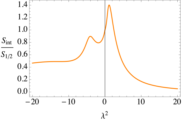
Figure 2: Plot of entropy $S_{\rm int}/S_{{\rm int},1/4}$ for the case $m\to 0$. We plot this against $\lambda^{2}$ (where we take $H=1$). This takes care of both $\pm\lambda^{2}$. In either case entanglement entropy is seen to decrease as non-locality strength increases.

5.3 $m\neq 0$ and $\lambda\neq 0$

In the case when both $m$ and $\lambda$ are non-zero then the entropy gets a more richer structure as there are two parameters. In the paper by [19] it was noticed that in local field theory as the mass decreases the long-range entanglement increases, which is a feature of deSitter. We decided to plot these cases to see the behaviour of entanglement entropy with varying $\lambda$ and $m$. This behaviour is depicted in figure 3.

  

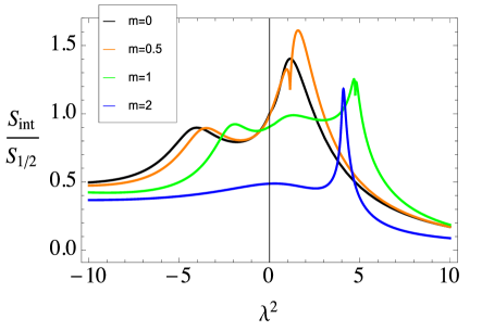
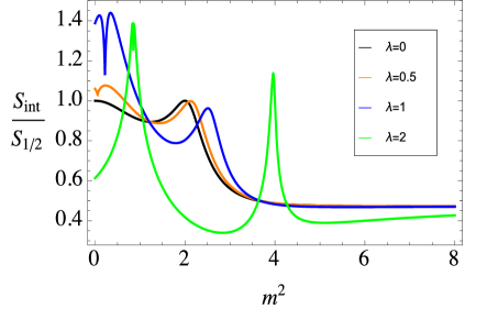
Figure 3: Plot of entropy $S_{\rm int}/S_{{\rm int},1/4}$ for varying $\lambda$ and $m$ (where we take $H=1$). It is seen that for small mass the entropy first increases then decreases as non-locality $\lambda$ increases.

6 Rényi entropy and negativity

From the density matrix and eigenvalues one can also define the corresponding Rényi-entropy which is defined as

$$S_{q}=\frac{1}{1-q}\log{\rm Tr}\left(\rho_{\rm red}^{q}\right)\,,\hskip 14.22636ptq>0\,,$$ (6.1)

where $\rho_{\rm red}$ is the reduced density matrix computed earlier. In the limit $q\to 1$ it reduces to the definition of entanglement entropy. The eigenvalues of the reduced density matrix are known and for our theory it is given in eq. (5.23). This then becomes

$$S_{q}=\frac{1}{1-q}\log\sum_{k}p_{k}^{q}\,.$$ (6.2)

For the eigenvalues $p_{k}$ given in eq. (5.23) one can perform the infinite summation easily as it is a geometric series. The expression for $S_{q}$ associated with each $SO(1,3)$ quantum number is given by,

$$S_{q}(p,\nu_{-},\nu_{+})=\frac{q}{1-q}\log(1-\lvert\gamma_{-}\rvert^{2})+\frac{q}{1-q}\log(1-\lvert\gamma_{+}\rvert^{2})-\frac{1}{1-q}\log\left(1-\lvert\gamma_{-}\gamma_{+}\rvert^{2q}\right)\,.$$ (6.3)

Then according as before we integrate $S_{q}(p,\nu_{-},\nu_{+})$ with the density of states for the $H^{3}$. This will give the piece of the Rényi entropy which contributes to long range

$$S_{q,{\rm int}}\equiv c_{6}=\frac{1}{\pi}\int_{0}^{\infty}{\rm d}p\,p^{2}S_{q}(p,\nu_{-},\nu_{+})\,.$$ (6.4)

Now various values of $q$ correspond to various interesting situations. For $q\to 0$, the Rényi entropy measures the dimension of the density matrix. It is also called Hartley entropy [41]. For $q\to 1/2$ one gets a very simple expression for the $S_{q}$.

$$S_{\frac{1}{2}}(p,\nu_{-},\nu_{+})=\log\left[\frac{(1-\lvert\gamma_{-}\rvert^{2})(1-\lvert\gamma_{+}\rvert^{2})}{\left(1-\lvert\gamma_{-}\gamma_{+}\rvert\right)^{2}}\right]\,.$$ (6.5)

In the case when $\nu_{-}=\nu_{+}=\nu$ then $S_{1/2}=0$. In figure 4 we plot the behaviour of Rényi entropy for various values of $q$ and massless non-local theory.

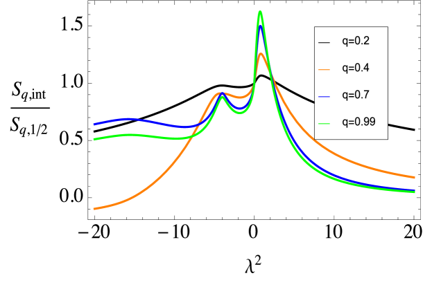
Figure 4: Plot of Rényi entropy $S_{{\rm q,int}}/S_{{\rm q,int},1/4}$ for varying $\lambda^{2}$ (where we take $H=1$). We plot the entropy for the case of $q=0.2$, $q=0.4$, $q=0.7$ and $q=0.99$. We consider the case of massless non-local theory.

The particular value of q$=1/2$ has relation with entanglement negativity, which is a measure of the quantum entanglement between the two regions [42, 43, 44]. For our case it can be defined using the full density matrix $\rho=\ket{\Psi}\bra{\Psi}$, where $\ket{\Psi}$ is given in eq. (5.12). If the basis for the $R$ and $L$ region is denoted by $R^{i}$ and $L^{i}$, then the transposed matrix $(\rho_{L})^{T}$ can be defined as $\bra{R^{i}L^{j}}(\rho_{L})^{T}\ket{R^{k}L^{m}}=\bra{R^{i}L^{m}}\rho\ket{R^{k}L^{j}}$. Using which one can express negativity as ${\cal E}\equiv\ln{\rm Tr}\lvert(\rho_{L})^{T}\rvert$ where ${\rm Tr}\lvert(\rho_{L})^{T}\rvert$ is the sum of the absolute value of the eigenvalues $(\rho_{L})^{T}$. For pure state [42] then the negativity equals the value corresponding to $q=1/2$. This then immediately gives the finite interesting piece of the negativity as [19]

$${\cal E}_{\rm intr}=\frac{1}{\pi}\int_{0}^{\infty}{\rm d}pp^{2}S_{1/2}(p,\nu_{-},\nu_{+})\,,$$ (6.6)

where $S_{1/2}(p,\nu_{-},\nu_{+})$ is given in eq. (6.5).

7 Conclusions

In this paper we explore a non-local scalar-field theory. We start by showing that this non-locality can also be obtained starting from a local coupled system of two scalars by integrating out one of the scalar field. We further show that this coupled system can actually be expressed as a system of decoupled scalar fields by a simple linear field transformation. In that sense the non-local system is equivalent to this. The aim of the paper is to seek an answer to question: how does the non-locality generated in infrared can affect or modify the low-energy physics of the system?

In cosmology we expect that there will exist entanglement beyond the Hubble radius, as in deSitter expanding space-time a particle pair which was initially created in causally connected region will eventually get separated and lie in causally disconnected regions of deSitter space-time. We know that quantum corrections lead to infrared non-locality in theories. So if the system begets a non-locality which becomes important in infrared then such non-locality is expected to have a role to play in affecting the entanglement between two disconnected regions of the deSitter space-time. With this motivation we investigate the change in behaviour of the entanglement due to the presence of infrared non-locality.

In local theories in flat space it is known that there is no long-range entanglement. However, in deSitter space it has been noticed in [19] that particle creation give rise to long-range entanglement. In local theories this feature is specific to deSitter space and doesn’t have any flat space counterpart. In this paper we are interested in exploring the modification this feature gets due to the presence of infrared non-locality and ask the question whether non-locality can have any non-trivial effect on such long-range entanglement?

Following the methodology described in the paper [19], we repeat the computation for the case of non-local massive scalar field theory. In the limit when non-locality strength goes to zero (i.e. when theory becomes local) we arrive at a local theory where the results are seen to be not in disagreement with the results obtained in [19]. In the case when we have non-locality in system then it adds an additional dimension into the problem. For massless theory, the presence of non-locality is seen to strongly affect the entanglement. This effect is however not monotonic in nature. As $\lambda^{2}$ is increased from zero to higher-values, it is noticed that the entanglement first increase, reaches a peak value and then decays. In the case when we change the sign of $\lambda^{2}\to-\lambda^{2}$ then an oscillating behaviour is witnessed in the long-range entanglement. This situation has been depicted in the figure 2. Such oscillations is due to the presence of tachyonic modes. This situation is gets more clear when one express the non-local system as a local system of decoupled scalars as expressed in eq. (2.8). Then the massless non-local case reduces to a very simple lagrangian of decoupled scalars with masses depending on $\lambda$. Then the case with decaying entanglement refers to decoupled scalars with complex masses, while the case of oscillating entanglement entropy refers to case of decoupled scalars with a tachyonic mass.

In the case when we have a massive non-local theory then the behaviour of entanglement entropy is more complicated in nature. This is depicted in figure 3. The qualitative features of this remains the same as in massless case although minute differences are noticed.

We then computed Rényi entropy for our case. As the density matrix for the system was known, so it allowed the computation of Rényi easily following the definition. We then studied the behaviour of $S_{q}$ with respect to non-locality strength $\lambda^{2}$ for various values of $q$. The qualitative features of $S_{q}$ are similar to the entanglement entropy: decaying for positive $\lambda^{2}$ and oscillating for $-\lambda^{2}$, although a flattening of figure is witnessed in case of lower values of $q$. This is depicted in figure 4.

The work presented here indicate the effect the presence of infrared non-locality will have on the entanglement between two disconnected regions of deSitter space-time. As infrared non-locality is an inevitable feature of well-defined quantum field theories, where it can naturally arise at low energies due to quantum corrections via renormalisation group running of parameters, therefore it means that infrared non-locality will have strong effect on the entanglement of disconnected regions. Hence, particle pair initially created in a causally connected region (inside Hubble radius) and later separated due to deSitter expansion (moved outside Hubble horizon) will be either strongly or weakly entangled depending on the nature of non-locality. This paper dealt with non-locality present in scalar field theory which play an important role in cosmology in understanding both early and late-time Universe. However, similar analysis can also be extended to field theories of other spin particles. This work sheds light on the importance of non-locality in the long-range entanglement and the significant role they will play in the deSitter phase of the cosmology.

Acknowledgements

GN will like to thank Nirmalya Kajuri for useful discussion. GN is supported by “Zhuoyue” (distinguished) Fellowship (ZYBH2018-03). H. Q. Z. is supported by the National Natural Science Foundation of China (Grants No. 11675140, No. 11705005, and No. 11875095).

References

- [1] L. Amico, R. Fazio, A. Osterloh and V. Vedral, Rev. Mod. Phys. 80, 517 (2008) doi:10.1103/RevModPhys.80.517 [quant-ph/0703044 [QUANT-PH]].
- [2] R. Horodecki, P. Horodecki, M. Horodecki and K. Horodecki, Rev. Mod. Phys. 81, 865 (2009) doi:10.1103/RevModPhys.81.865 [quant-ph/0702225].
- [3] L. Bombelli, R. K. Koul, J. Lee and R. D. Sorkin, Phys. Rev. D 34, 373 (1986). doi:10.1103/PhysRevD.34.373
- [4] M. Srednicki, Phys. Rev. Lett. 71, 666 (1993) doi:10.1103/PhysRevLett.71.666 [hep-th/9303048].
- [5] G. Narain and N. Kajuri, arXiv:1812.00948 [hep-th].
- [6] M. Maggiore, Phys. Rev. D 93, no. 6, 063008 (2016) doi:10.1103/PhysRevD.93.063008 [arXiv:1603.01515 [hep-th]].
- [7] M. Maggiore, Fundam. Theor. Phys. 187, 221 (2017) doi:10.1007/978-3-319-51700-116 [arXiv:1606.08784 [hep-th]].
- [8] G. Narain and T. Li, Phys. Rev. D 97, no. 8, 083523 (2018) doi:10.1103/PhysRevD.97.083523 [arXiv:1712.09054 [hep-th]].
- [9] G. Narain and T. Li, Universe 4, no. 8, 82 (2018) doi:10.3390/universe4080082 [arXiv:1807.10028 [hep-th]].
- [10] J. W. Moffat, Eur. Phys. J. Plus 126, 43 (2011) doi:10.1140/epjp/i2011-11043-7 [arXiv:1008.2482 [gr-qc]].
- [11] T. Biswas, T. Koivisto and A. Mazumdar, JCAP 1011, 008 (2010) doi:10.1088/1475-7516/2010/11/008 [arXiv:1005.0590 [hep-th]].
- [12] L. Modesto, Phys. Rev. D 86, 044005 (2012) doi:10.1103/PhysRevD.86.044005 [arXiv:1107.2403 [hep-th]].
- [13] L. Modesto and L. Rachwal, Nucl. Phys. B 889, 228 (2014) doi:10.1016/j.nuclphysb.2014.10.015 [arXiv:1407.8036 [hep-th]].
- [14] L. Modesto and L. Rachwa?, Int. J. Mod. Phys. D 26, no. 11, 1730020 (2017). doi:10.1142/S0218271817300208
- [15] N. Kajuri, Phys. Rev. D 95, no. 10, 101701 (2017) doi:10.1103/PhysRevD.95.101701 [arXiv:1704.03793 [gr-qc]].
- [16] N. Kajuri and D. Kothawala, arXiv:1806.10345 [gr-qc].
- [17] N. Kajuri and G. Narain, arXiv:1812.00946 [hep-th].
- [18] G. Narain and N. Kajuri, arXiv:1812.00947 [hep-th].
- [19] J. Maldacena and G. L. Pimentel, JHEP 1302, 038 (2013) doi:10.1007/JHEP02(2013)038 [arXiv:1210.7244 [hep-th]].
- [20] R. E. Cutkosky, P. V. Landshoff, D. I. Olive and J. C. Polkinghorne, Nucl. Phys. B 12, 281 (1969). doi:10.1016/0550-3213(69)90169-2
- [21] T. D. Lee and G. C. Wick, Nucl. Phys. B 9, 209 (1969). doi:10.1016/0550-3213(69)90098-4
- [22] H. Yamamoto, Prog. Theor. Phys. 44, 272 (1970). doi:10.1143/PTP.44.272
- [23] K. L. Nagy, Acta Phys. Hung. 29, 251 (1970). doi:10.1007/BF03155840
- [24] N. A. Chernikov and E. A. Tagirov, Ann. Inst. H. Poincare Phys. Theor. A 9, 109 (1968).
- [25] T. S. Bunch and P. C. W. Davies, Proc. Roy. Soc. Lond. A 360, 117 (1978). doi:10.1098/rspa.1978.0060
- [26] J. B. Hartle and S. W. Hawking, Phys. Rev. D 28, 2960 (1983) [Adv. Ser. Astrophys. Cosmol. 3, 174 (1987)]. doi:10.1103/PhysRevD.28.2960
- [27] C. G. Callan, Jr. and F. Wilczek, Phys. Lett. B 333, 55 (1994) doi:10.1016/0370-2693(94)91007-3 [hep-th/9401072].
- [28] S. Kanno, J. Murugan, J. P. Shock and J. Soda, JHEP 1407, 072 (2014) doi:10.1007/JHEP07(2014)072 [arXiv:1404.6815 [hep-th]].
- [29] N. Iizuka, T. Noumi and N. Ogawa, Nucl. Phys. B 910, 23 (2016) doi:10.1016/j.nuclphysb.2016.06.024 [arXiv:1404.7487 [hep-th]].
- [30] S. Kanno, JCAP 1407, 029 (2014) doi:10.1088/1475-7516/2014/07/029 [arXiv:1405.7793 [hep-th]].
- [31] S. Kanno, J. P. Shock and J. Soda, JCAP 1503, 015 (2015) doi:10.1088/1475-7516/2015/03/015 [arXiv:1412.2838 [hep-th]].
- [32] S. Kanno, M. Sasaki and T. Tanaka, JHEP 1703, 068 (2017) doi:10.1007/JHEP03(2017)068 [arXiv:1612.08954 [hep-th]].
- [33] S. Kanno, J. P. Shock and J. Soda, Phys. Rev. D 94, no. 12, 125014 (2016) doi:10.1103/PhysRevD.94.125014 [arXiv:1608.02853 [hep-th]].
- [34] S. Kanno and J. Soda, Phys. Rev. D 96, no. 8, 083501 (2017) doi:10.1103/PhysRevD.96.083501 [arXiv:1705.06199 [hep-th]].
- [35] I. V. Vancea, Nucl. Phys. B 924, 453 (2017) doi:10.1016/j.nuclphysb.2017.09.017 [arXiv:1609.02223 [hep-th]].
- [36] S. Choudhury and S. Panda, Eur. Phys. J. C 78, no. 1, 52 (2018) doi:10.1140/epjc/s10052-017-5503-4 [arXiv:1708.02265 [hep-th]].
- [37] S. Bhattacharya, S. Chakrabortty and S. Goyal, arXiv:1812.07317 [hep-th].
- [38] M. Bucher, A. S. Goldhaber and N. Turok, Phys. Rev. D 52, 3314 (1995) doi:10.1103/PhysRevD.52.3314 [hep-ph/9411206].
- [39] M. Sasaki, T. Tanaka and K. Yamamoto, Phys. Rev. D 51, 2979 (1995) doi:10.1103/PhysRevD.51.2979 [gr-qc/9412025].
- [40] A. A. Bytsenko, G. Cognola, L. Vanzo and S. Zerbini, Phys. Rept. 266, 1 (1996) doi:10.1016/0370-1573(95)00053-4 [hep-th/9505061].
- [41] M. Headrick, Phys. Rev. D 82, 126010 (2010) doi:10.1103/PhysRevD.82.126010 [arXiv:1006.0047 [hep-th]].
- [42] G. Vidal and R. F. Werner, Phys. Rev. A 65, 032314 (2002). doi:10.1103/PhysRevA.65.032314
- [43] P. Calabrese, J. Cardy and E. Tonni, Phys. Rev. Lett. 109, 130502 (2012) doi:10.1103/PhysRevLett.109.130502 [arXiv:1206.3092 [cond-mat.stat-mech]].
- [44] P. Calabrese, J. Cardy and E. Tonni, J. Stat. Mech. 1302, P02008 (2013) doi:10.1088/1742-5468/2013/02/P02008 [arXiv:1210.5359 [cond-mat.stat-mech]].