Constraining heavy neutral gauge boson $Z^{\prime}$ in the 3 - 3 - 1 models by weak charge data of Cesium and proton

Abstract

The recent experimental data of the weak charges of Cesium and proton is analyzed in the framework of the models based on the $\mbox{SU}(3)_{C}\times\mbox{SU}(3)_{L}\times\mbox{U}(1)_{X}$ (3-3-1) gauge group, including the 3-3-1 model with CKS mechanism (3-3-1CKS) and the general 3-3-1 models with arbitrary $\beta$ (3-3-1$\beta$) with three Higgs triplets. We will show that at the TeV scale, the mixing among neutral gauge bosons plays significant effect. Within the present values of the weak charges of Cesium and proton we get the lowest mass bound of the extra heavy neutral gauge boson to be 1.27 TeV. The results derived from the weak charge data, perturbative limit of Yukawa coupling of the top quark, and the relevant Landau poles favor the models with $\beta=\pm\frac{1}{\sqrt{3}}$ and $\beta=0$ while ruling out the ones with $\beta=\pm\sqrt{3}$. In addition, there are some hints showing that in the 3-3-1 models, the third quark family should be treated differently from the first twos.

Keywords: Extensions of electroweak gauge sector, Extensions of electroweak Higgs sector

I Introduction

Nowadays, the experimental data on neutrino masses and mixing as well as on Dark Matter (DM) lead to fact that the Standard Model (SM) must be extended. Among the beyond SM extensions, the models based on the $\mbox{SU}(3)_{C}\times\mbox{SU}(3)_{L}\times\mbox{U}(1)_{X}$ gauge group Valle:1983dk ; Pisano:1991ee ; Frampton:1992wt ; Foot:1992rh ; Foot:1994ym ; Hoang:1995vq ; Hoang:1996gi (3 - 3 - 1 models) are attractive in the following senses. First of all, these models are concerned with the search of an explanation for the number of fermion generations to be three, when the QCD asymptotic freedom is combined. Some other advantages of the 3-3-1 models are: i) the electric charge quantization is solved deSousaPires:1998jc ; VanDong:2005ux , ii) there are several sources of CP violation Montero:1998yw ; Montero:2005yb , and iii) the strong-CP problem is solved due to the natural Peccei-Quinn symmetry Pal:1994ba ; Dias:2002gg ; Dias:2003zt ; Dias:2003iq .

There are two main versions of the 3 - 3 - 1 models which depend on the parameter $\beta$ in the electric charge operator

$$Q=T_{3}+\beta T_{8}+X\,.$$ (1)

If $\beta=\sqrt{3}$, this is the minimal version Pisano:1991ee ; Frampton:1992wt ; Foot:1992rh , and $\beta=-\frac{1}{\sqrt{3}}$ corresponds to the 3-3-1 model with right-handed neutrinos Valle:1983dk ; Foot:1994ym ; Hoang:1995vq ; Hoang:1996gi .

At present, we still face an old problem of explanation of hierarchies and structure of the fermion sector. However, in the above models, most researches on the 3-3-1 models are not concerned with vast different masses among the generations (see references in Ref.CarcamoHernandez:2017cwi ). It is well known that the Yukawa interactions are not enough for producing fermion masses and mixings. According to our best of knowledge, the first work for solving the mentioned puzzles in quark sector is in Ref. Froggatt:1978nt named Froggatt-Nielsen mechanism. Recently, the new mechanism based on sequential loop suppression mechanism, is more natural since its suppression factor is arisen from loop factor $l\approx(1/4\pi)^{2}$. The above mentioned mechanism is called by CKS - the names of its authors CarcamoHernandez:2016pdu . The Froggatt-Nielsen mechanism was implemented to the 3-3-1 model in Ref. Huitu:2017ukq . In recent work Ref.  CarcamoHernandez:2017cwi the CKS mechanism has been implemented to the 3-3-1 model with $\beta=-\frac{1}{\sqrt{3}}$, and it is interesting to note that the derived model is renormalizable. We name it the 3-3-1 CKS model for short. In the Ref. Long:2018dun , the Higgs and gauge sectors of the model are explored. From the experimental data on the $\rho$ parameter, the bound on the scale of the first step of the spontaneous symmetry breaking (SSB) in the 3-3-1 CKS is in the range of 6 TeV Long:2018dun . There also exist helpful relations among masses of gauge bosons, this is essential point for the model phenomenology.

At present, the new neutral gauge boson $Z^{\prime}$ is a very attractive subject in Particle Physics due to potential discovery of right-handed neutrinos through its mediation Freitas:2018vnt . Within its mass around 2.5 TeV, the simulation shows that it may be discovered at the LHC. Hence it is necessary to study more deeply different aspects to fix the mass as well as properties of $Z^{\prime}$. To fix the model parameters, one often looks at well known observables such as the $\rho$ parameter, mass differences of neutral mesons, and deviation of weak charge of nucleus, etc. So, in this paper we focus on the latter subject.

Recently, new constraints of the $Z^{\prime}$ mass around 4 TeV have been reported from studying the $Z^{\prime}$ decays into the SM lepton pairs, based on the new LHC Run 2 data Aaboud:2017buh ; Aaboud:2017sjh ; Sirunyan:2018exx ; Aad:2019fac . On the other hand, a recent study on a particular 3-3-1 model argued that the lower bounds of $Z^{\prime}$ mass can be significantly smaller than those obtained from LHC, if other decay channels of $Z^{\prime}$ into new particles are included Coriano:2018coq . We will follow this particular framework, i.e. the new constraints of $Z^{\prime}$ will be omitted in our discussion. A more general dependence of the lower bounds of $Z^{\prime}$ mass in 3-3-1 models on the LHC data will be studied in the future.

The parity violation in weak interactions was known for long time ago. In the SM, it can be seen from the atomic parity violation (APV) caused by the neutral gauge boson $Z$. In the beyond Standard Model (BSM), the APV gets additional contribution from new heavy neutral gauge bosons $Z^{\prime}$. Therefore, the data on APV, especially of the Cesium (${}^{133}_{55}Cs$) being stable atom, is an effective channel for probing the new neutral gauge boson $Z^{\prime}$. This is our aim in this work.

The experimental data on the APV in Cesium atom Bennett:1999pd has caused extensive interest and reviews Rosner:2001ck ; Ginges:2003qt ; Bouchiat:2004sp ; Guena:2005uj ; Davoudiasl:2012qa ; Erler:2014fqa . Parity violation in the SM results from exchanges of weak gauge bosons, namely, in electron-hadron neutral-current processes. The parity violation is due to the vector axial-vector interaction in the effective Lagrangian. The measurement is stated in terms of the weak charge $Q_{W}$, which parameterizes the parity violating Lagrangian. Due to the extra neutral gauge bosons, in the BSM, the weak charge of an isotope (X) gets additional value which is called by deviation defined as follows

$$\Delta Q_{W}(^{A}_{Z}X)\equiv Q_{W}^{\mathrm{BSM}}(^{A}_{Z}X)-Q_{W}^{\mathrm{SM}}(^{A}_{Z}X)\,.$$ (2)

For the concrete stable isotope Cesium (Cs), it is reported recently from experiment as Dzuba:2012kx ; Tanabashi:2018oca

$$Q^{\mathrm{exp}}_{W}(^{133}_{55}{\mathrm{C}s})=-72.62\pm 0.43.$$ (3)

Comparing to the SM prediction $Q_{W}^{\mathrm{SM}}(^{133}_{55}Cs)=-73.23\pm 0.01$ Erler:2013xha ; Tanabashi:2018oca yields the deviation $\Delta Q_{W}$ as follows Dzuba:2012kx

$$\Delta Q_{W}(^{133}_{55}Cs)\equiv Q^{\mathrm{exp}}_{W}(^{133}_{55}{\mathrm{C}s})-Q_{W}^{\mathrm{S}M}(^{133}_{55}{\mathrm{C}s})=0.61\pm 0.43\,,$$ (4)

which is $1.4~{}\sigma$ away from the SM prediction. This value has been widely used for analysis of possible new physics, where it is assumed that the BSM can be explained the experimental value of the weak charge $Q_{W}(^{133}_{55}Cs)$.

On the other hand, the weak charge of an atom is formulated as a function of the two independent contributions of light quarks $u$ and $d$, the experimental weak charge values of the two distinguishable isotopes will result in different allowed regions of the parameter space defined by a BSM. Hence, combining result of allowed regions from experimental weak charge data of Cesium and proton will be more strict than the previous one. Recently, the experiments of parity-violation in electron scattering (PVES), see a review in Souder:2015mlu , have determined the latest value of the proton’s weak charge, namely $Q^{\mathrm{exp}}_{W}(^{1}_{1}p)=0.0719\pm 0.0045$ Androic:2018kni . It was shown to be in great agreement with the SM prediction, $Q^{\mathrm{SM}}_{W}(^{1}_{1}p)=0.0708\pm 0.0003$. The deviation from the SM is

$$\Delta Q_{W}(^{1}_{1}p)=0.0011\pm 0.0045.$$ (5)

Considering a BSM containing an additional heavy neutral gauge boson $Z^{\prime}$ apart from the SM one $Z$, a theoretical deviation of $Q_{W}$ from the SM prediction for an isotope ${}^{A}_{Z}X$ is given by

$$\Delta Q^{\mathrm{BSM}}_{W}(^{A}_{Z}X) \simeq \left[2Z-A+4Z\left(\frac{s_{W}^{4}}{1-2s^{2}_{W}}\right)\right]\Delta\rho$$

$$+ 4s_{\phi}\left\{(A+Z)\left[g_{A}(e)g^{\prime}_{V}(u)+g^{\prime}_{A}(e)g_{V}(u)\right]\right.$$

$$+ \left.(2A-Z)\left[g_{A}(e)g^{\prime}_{V}(d)+g^{\prime}_{A}(e)g_{V}(d)\right]\right\}$$

$$- 4\left(\frac{M_{Z_{1}}^{2}}{M^{2}_{Z_{2}}}\right)[(A+Z)g^{\prime}_{A}(e)g^{\prime}_{V}(u)+(2A-Z)g^{\prime}_{A}(e)g^{\prime}_{V}(d)],$$

where $s_{\phi}\equiv\sin\phi$ corresponds to the $Z-Z^{\prime}$ mixing of the SM and new heavy neutral gauge bosons $Z$ and $Z^{\prime}$ that create the two physical states $Z_{1,2}$ with masses $M_{Z_{1,2}}$.

Notations in Eq. (I) are based on the vector-axial (V-A) currents of neutral gauge bosons defined by the well-known Lagrangian

$$\mathcal{L}_{Vff} = \frac{g}{2c_{W}}\sum_{f}\overline{f}\gamma^{\mu}(g_{V}(f)-\gamma_{5}g_{A}(f)fZ_{\mu}$$ (7)

$$+ \frac{g}{2c_{W}}\sum_{f}\overline{f}\gamma^{\mu}(g^{\prime}_{V}(f)-\gamma_{5}g^{\prime}_{A}(f)fZ^{\prime}_{\mu},$$

where the summation is taken over the fermions of the BSM, $g=e/s_{W}$ is the $SU(2)_{L}$ gauge coupling of the SM.

The formula (I) has been checked in details by us (see appendix A) based on original calculation in Ref. Altarelli:1991ci that concerned for $U(1)$ gauge extensions of the SM. However, it is also valid for other non-Abelian gauge extensions including 3-3-1 models Hoang:2000jy ; CarcamoHernandez:2005ka ; Gutierrez:2005rq ; Dong:2006cn ; Salazar:2007ym ; Gauld:2013qja ; Buras:2013dea ; Martinez:2014lta . Especially, the formulas for arbitrary $\beta$ given in Ref. CarcamoHernandez:2005ka was corrected in Ref. Martinez:2014lta following a recent correction of $Z-Z^{\prime}$ mixing angle Buras:2014yna . Using the same notations our formula (I) contains two factors 4 instead of 16 in the expression of the weak charge used in Ref. Martinez:2014lta . Additionally, the numerical investigation in Ref. Martinez:2014lta used the old experimental data of the Cs weak charge Beringer:1900zz , which is very well consistent with the SM prediction. On the other hand, the new constraint given in Eq. (3) is significantly different from the previous Beringer:1900zz , and implies a certain deviation from the SM. Therefore, a new investigation based on the latest experimental data of both weak charges of Cesium and proton will result in new information of allowed regions of the parameter spaces in the 3-3-1 models.

Taking into account the SM gauge couplings

$$g_{A}(e)=-\frac{1}{2}\,,\hskip 8.5359ptg_{V}(u)=\frac{1}{2}-\frac{4s_{W}^{2}}{3}\,,\hskip 8.5359ptg_{V}(d)=-\frac{1}{2}+\frac{2s_{W}^{2}}{3}\,;$$ (8)

the experimental value of the Weinberg angle at the $M_{Z}$ scale Tanabashi:2018oca $s_{W}^{2}=0.23122$, $\left(\frac{s_{W}^{4}}{1-2s^{2}_{W}}\right)=0.0994544$; and the scale dependence of the gauge couplings $g$ in Eq. (7), the expression (I) is written in the more general form

$$\Delta Q^{\mathrm{BSM}}_{W}(^{A}_{Z}X) \simeq -\left(A-2.39782\times Z\right)\Delta\rho$$

$$- 2s_{\phi}\left\{A\left[2g^{\prime}_{V}(d)+g^{\prime}_{V}(u)+g^{\prime}_{A}(e)\right]\right.$$

$$- \left.Z\left[g^{\prime}_{A}(e)\times 1.07512+g^{\prime}_{V}(d)-g^{\prime}_{V}(u)\right]\right\}\times\frac{g(M_{Z_{2}})}{g(M_{Z_{1}})}$$

$$- 4g^{\prime}_{A}(e)\left(\frac{M_{Z_{1}}^{2}}{M^{2}_{Z_{2}}}\right)\left\{A\left[2g^{\prime}_{V}(d)+g^{\prime}_{V}(u)\right]+Z\left[g^{\prime}_{V}(u)-g^{\prime}_{V}(d)\right]\right\}\times\frac{g^{2}(M_{Z_{2}})}{g^{2}(M_{Z_{1}})}\,,$$

where $g(M_{Z_{1,2}})$ are respective gauge couplings of the $Z_{1,2}$ at their mass scales. We emphasize that Eq. (I) contains major improvements from the original version Altarelli:1991ci , see detailed discussion in appendix A. The above formula is also applicable for the models based on $\mbox{SU}(3)_{C}\times\mbox{SU}(3)_{L}\times\mbox{U}(1)_{X}$ gauge group, where effect of scale dependence was mentioned but the $Z-Z^{\prime}$ mixing was ignored Gauld:2013qja ; Buras:2013dea . The subject was also considered earlier in Refs. Hoang:2000jy ; Dong:2006cn , but for only the minimal and economical 3-3-1 versions, respectively. The formula (I) is different from those used to investigate APV in 3-3-1 models in Refs. Martinez:2014lta , where the scale dependence of neutral gauge couplings are also taken into account. Furthermore, in the light of new experimental results of weak charges and rho parameter Tanabashi:2018oca , the parameter spaces of the 3-3-1 models will be re-investigated. Instead of Ref. Martinez:2014lta , where only model C introduced in Ref. Martinez:2006gb was paid attention using the APV of $Q_{W}(Cs)$, we will discuss all allowed regions of the three parameter spaces corresponding to the three models A, B, and C, based on the latest experimental data of both $Q_{W}(Cs)$ and $Q_{W}(p)$. The effects of the perturbative limit of top quark Yukawa coupling on the parameter space will also be included. The combination resulting from the three mentioned ingredients will affect differently the parameter spaces of the three 3-3-1 models A,B,C. Hence, it may suggest which models can be survived or ruled out, instead of the common acceptance in literature that prefers the model A, where the heavy quark family containing the top quark is treated differently from the two lighter ones.

The further plan of this paper is as follows. Sect. II is devoted to the 3-3-1 CKS model where the particle content is introduced. In this section, the gauge boson masses and mixing are also discussed, and the couplings between neutral gauge bosons $Z$ and $Z^{\prime}$ and fermions are presented. In Sect. II.3, we consider the deviation of weak charge for Cesium in the 3-3-1 CKS, from which the lower bound on the $M_{Z_{2}}$ is derived. Sect. III is devoted for the model 3-3-1$\beta$ Ochoa:2005ih ; CarcamoHernandez:2005ka . In this section, we will focus on different kinds of quark assignments listed in Ref. CarcamoHernandez:2005ka , where the heavy flavor quarks $t$ and $b$ behave differently from other ones (representation A) or the light quarks $u$ and $d$ do the same (representation C). The analytic expressions of the deviations $\Delta Q^{\mathrm{BSM}}_{W}(^{A}_{Z}X)$ predicted by the models will be combined with the latest data of APV and PVES to investigate allowed regions of the parameter spaces, which can result in the possibility of surviving or ruling out the model under consideration. We make a conclusion in the last section - section IV. Two appendices show in detailed steps how to derive the analytic expressions of the weak charges in the general case and the particular case of the 3-3-1$\beta$ model.

II Atomic parity violation in the 3 - 3 - 1 CKS model

In this section the needed ingredients for investigating the weak charges predicted by the 3-3-1 CKS model are discussed.

II.1 Particle content

As in the ordinary 3-3-1 model without exotic electric charges, the quark sector contains two quark generations transforming as antitriplet and one remaining generation transforming as triplet under $SU(3)_{L}$ subgroup. The other extra quarks transform as singlet under above mentioned subgroup. The quantum numbers of the quark sector are summarized in Table 1.

Table 1: Quark assignments under $SU(3)_{L},U(1)_{X},U(1)_{L_{g}},Z_{4},Z_{2}$ and the values of generalized lepton number $L_{g}$ (all quarks are in triplets under $SU(3)_{C}$)

	$Q_{1L}$	$Q_{2L}$	$Q_{3L}$	$U_{1R}$	$U_{2R}$	$U_{3R}$	$T_{R}$	$D_{1R}$	$D_{2R}$	$D_{3R}$	$J_{1R}$	$J_{2R}$	$\widetilde{T}_{1L}$	$\widetilde{T}_{1R}$	$\widetilde{T}_{2L}$	$\widetilde{T}_{2R}$	$B_{L}$	$B_{R}$
$SU(3)_{L}$	$3^{*}$	$3^{*}$	$3$	1	1	1	1	1	1	1	1	1	1	1	1	1	1	1
$X$	0	0	$\frac{1}{3}$	$\frac{2}{3}$	$\frac{2}{3}$	$\frac{2}{3}$	$\frac{2}{3}$	$-\frac{1}{3}$	$-\frac{1}{3}$	$-\frac{1}{3}$	$-\frac{1}{3}$	$-\frac{1}{3}$	$\frac{2}{3}$	$\frac{2}{3}$	$\frac{2}{3}$	$\frac{2}{3}$	$-\frac{1}{3}$	$-\frac{1}{3}$
$L_{g}$	$\frac{2}{3}$	$\frac{2}{3}$	$-\frac{2}{3}$	$0$	$0$	$0$	$-2$	$0$	$0$	$0$	$2$	$2$	$0$	$0$	$0$	$0$	$0$	$0$
$Z_{4}$	$-1$	$-1$	$1$	$1$	$-i$	$1$	$1$	$1$	$1$	$1$	$-1$	$-1$	$i$	$1$	$i$	$1$	$-1$	$-1$
$Z_{2}$	$1$	$1$	$1$	$1$	$1$	$-1$	$-1$	$1$	$1$	$1$	$-1$	$-1$	$1$	$1$	$1$	$1$	$1$	$1$

As seen from Table 1, in the model under consideration, all extra quarks have electric charges of quarks in the SM. As shown in Ref. CarcamoHernandez:2017cwi , the spontaneous symmetry breaking (SSB) provides masses for only extra quarks as well as top quark. The remaining quarks get masses by radiative corrections. To explain why top quark gets mass at the tree level but bottom quark does not get, the reason lies in the behaviour of their right-handed components under the symmetry $Z_{2}$: $U_{3R}$ is odd, while $D_{3R}$ is even. It is crucial for the forbiddance of unwanted terms.

The content of the leptonic sector is summarized in Table 2. As in the quark sector, the extra leptons: $E_{i},i=1,2,3$, $N_{i},i=1,2,3$ and $\Psi_{R}$ get masses at the tree level. Table 2 also shows that under the $Z_{2}$, right-handed components of the charged leptons in the second (muon) and the third (tauon) generations are even, while for the first generation, it is odd. That is why tauon and muon get masses at the one-loop level, but the electron gets mass at two-loop correction CarcamoHernandez:2017cwi . Table 2 also shows that the extra neutral leptons $N_{i},i=1,2,3$ have lepton number opposite to those of ordinary leptons.

Table 2: Lepton assignments under $SU(3)_{L},U(1)_{X},U(1)_{L_{g}},Z_{4},Z_{2}$ and the values of generalized lepton number $L_{g}$ (all leptons are singlets under $SU(3)_{C}$)

	$L_{1L}$	$L_{2L}$	$L_{3L}$	$e_{1R}$	$e_{2R}$	$e_{3R}$	$E_{1L}$	$E_{2L}$	$E_{3L}$	$E_{1R}$	$E_{2R}$	$E_{3R}$	$N_{1R}$	$N_{2R}$	$N_{3R}$	$\Psi_{R}$
$SU(3)_{L}$	3	3	3	1	1	1	1	1	1	1	1	1	1	1	1	1
$X$	$-\frac{1}{3}$	$-\frac{1}{3}$	$-\frac{1}{3}$	-1	-1	-1	-1	-1	-1	-1	-1	-1	0	0	0	0
$L_{g}$	$\frac{1}{3}$	$\frac{1}{3}$	$\frac{1}{3}$	$1$	$1$	$1$	$1$	$1$	$1$	$1$	$1$	$1$	$-1$	$-1$	$-1$	$1$
$Z_{4}$	$i$	$i$	$i$	$-i$	$-i$	$-i$	$1$	$i$	$i$	$-i$	$-i$	$-i$	$i$	$i$	$i$	$1$
$Z_{2}$	$-1$	$1$	$1$	$-1$	$1$	$1$	$-1$	$1$	$1$	$-1$	$1$	$1$	$-1$	$-1$	$-1$	$-1$

The Higgs sector contains three scalar triplets $\chi$, $\eta$ and $\rho$ and seven singlets $\varphi_{1}^{0}$,$\ \varphi_{2}^{0}$, $\xi^{0}$,$\ \phi_{1}^{+}$,$\ \phi_{2}^{+}$, $\phi_{3}^{+}$ and $\phi_{4}^{+}$. The content of the Higgs sector is presented in Table 3.

Table 3: Scalar assignments under $SU(3)_{L},U(1)_{X},U(1)_{L_{g}},Z_{4},Z_{2}$ and the values of generalized lepton number $L_{g}$.

	$\chi$	$\eta$	$\rho$	$\varphi_{1}^{0}$	$\varphi_{2}^{0}$	$\phi_{1}^{+}$	$\phi_{2}^{+}$	$\phi_{3}^{+}$	$\phi_{4}^{+}$	$\xi^{0}$
$SU(3)_{L}$	3	3	3	1	1	1	1	1	1	1
$X$	$-\frac{1}{3}$	$-\frac{1}{3}$	$\frac{2}{3}$	0	0	1	1	1	1	0
$L_{g}$	$\frac{4}{3}$	$-\frac{2}{3}$	$-\frac{2}{3}$	$0$	$0$	$0$	$-2$	$-2$	$-2$	$-2$
$Z_{4}$	$1$	$1$	$-1$	$-1$	$i$	$i$	$-1$	$-1$	$1$	$1$
$Z_{2}$	$-1$	$-1$	$1$	$1$	$1$	$1$	$1$	$-1$	$-1$	$1$

We note that, in contradiction with ordinary 3-3-1 model, the neutral component of the $\rho$ triplet does not have a vacuum expectation value (VEV). That is why the charged leptons do not get masses at the tree level. From Table 3, it follows that $\chi$ triplet has generalized lepton number $L_{g}$ CarcamoHernandez:2017cwi ; Chang:2006aa different from those of $\eta$ and $\rho$ triplets. This leads to the fact that the bottom elements of the $\eta$ and $\rho$ triplets as well as two first rows of the $\chi$ have lepton number equal to 2, the same as $\phi^{+}_{i},i=2,3,4$ and $\xi$ do.

To close this section, we remind that after SSB, the charged and non-Hermitian gauge bosons get masses as below  Long:2018dun

$$m^{2}_{W}=\frac{g^{2}}{4}v_{\eta}^{2}\,,\hskip 8.5359ptM^{2}_{X^{0}}=\frac{g^{2}}{4}\left(v^{2}_{\chi}+v_{\eta}^{2}\right)\,,\hskip 8.5359ptM^{2}_{Y}=\frac{g^{2}}{4}v_{\chi}^{2}\,,$$ (10)

where we have used the following notations

$$W_{\mu}^{\pm}=\frac{1}{\sqrt{2}}\left(A_{\mu 1}\mp iA_{\mu 2}\right)\,,\hskip 8.5359ptY_{\mu}^{\pm}=\frac{1}{\sqrt{2}}\left(A_{\mu 6}\pm iA_{\mu 7}\right)\,,\hskip 8.5359ptX_{\mu}^{0}=\frac{1}{\sqrt{2}}\left(A_{\mu 4}-iA_{\mu 5}\right)\,.$$ (11)

From (11), the following consequences are in order

$$v_{\eta}=v=246\,\textrm{GeV}\,,$$ (12)

$$M^{2}_{X^{0}}-M^{2}_{Y}=m^{2}_{W}\,.$$ (13)

Note that the value $\Delta Q_{W}$ depends on couplings of neutral gauge bosons $Z$ and $Z^{\prime}$ with light quark $u$ and $d$. Hence, we turn to the neutral current sector of the model.

II.2 Neutral currents

Looking at Eq. (47), one recognizes that some couplings between fermions and neutral gauge bosons $Z,Z^{\prime}$ enter to the discrepancies. The needed interactions between fermions and gauge bosons are followed from a piece

$$L_{\mbox{fermion \& gauge boson}}\supset\sum_{f}i\overline{f}\gamma^{\mu}D_{\mu}f\,.$$ (14)

Here, the covariant derivative is defined by

$$D_{\mu}=\partial_{\mu}-igA_{\mu a}T_{a}-ig_{X}XT_{9}B_{\mu}\,,$$ (15)

where $g$ and $g_{X}$ are the gauge coupling constants of the $SU(3)_{L}$ and $U(1)_{X}$ groups, respectively. Here, $T_{a}$ ($a=1,2,..,9$) are the generators of the $SU(3)$ group with gauge bosons $A_{\mu a}$. Corresponding to the $SU(3)_{L}$ representations, namely triplet, antitriplet, or singlet of the fermion, $T_{a}=\frac{1}{2}\lambda_{a},-\frac{1}{2}\lambda^{T}_{a}$, or $0$. Furthermore, we choose the $U(1)_{X}$ generator as $T_{9}=1/\sqrt{6}\text{ diag}(1,1,1)$ for both triplet and antitriplet, while $T_{9}=1/\sqrt{6}$ for singlets. For the convenience, one rewrites (15) as follows

$$D_{\mu}=\partial_{\mu}-igP_{\mu}^{CC}-igP_{\mu}^{NC}\,,$$ (16)

where

$$P_{\mu}^{CC}=\sum_{a=1,2,4,5,6,7}T_{a}A_{\mu a}\,,$$ (17)

and $P_{\mu}^{NC}$ is determined from diagonal generators, namely

$$P_{\mu}^{NC}=\sum_{a=3,8}T_{a}A_{\mu a}+tXT_{9}B_{\mu},\,\hskip 8.5359ptt\equiv\frac{g_{X}}{g}=\frac{3\sqrt{2}\sin\theta_{W}(M_{Z^{\prime}})}{\sqrt{3-4\sin^{2}\theta_{W}(M_{Z^{\prime}})}}\,.$$ (18)

Since atom cesium is only composed of light quarks, namely $u$ and $d$ quarks and electron, therefore, we just need to deal with these fermions. The coupling constants relevant for calculations of APV in the cesium atom for the SM and the 3 - 3 - 1 CKS model are presented in Table 4.

Table 4: Vector and axial-vector coupling constants relevant for APV in the SM and 3 - 3 - 1 CKS model

Standard Model	3-3-1 CKS model
$g_{A}(e)=-\frac{1}{2}$	$g^{\prime}_{A}(e)=+\frac{1}{2\sqrt{3-4s^{2}_{W}}}$
$g_{V}(u)=\frac{1}{2}-\frac{4s_{W}^{2}}{3}$	$g^{\prime}_{V}(u)=\frac{-3+8s_{W}^{2}}{6\sqrt{3-4s_{W}^{2}}}$
$g_{V}(d)=-\frac{1}{2}+\frac{2s_{W}^{2}}{3}$	$g^{\prime}_{V}(d)=\frac{-3+2s_{W}^{2}}{6\sqrt{3-4s_{W}^{2}}}$

In the limit $v_{\chi}\gg v_{\eta}$, the $Z-Z^{\prime}$ mixing angle is Long:2018dun

$$\tan\phi\simeq\frac{(1-2s_{W}^{2})\sqrt{3-4s^{2}_{W}}}{4c^{4}_{W}}\left(\frac{v_{\eta}^{2}}{v_{\chi}^{2}}\right)\,.$$ (19)

II.3 Deviation of the weak charge expression in the 3-3-1 CKS model

Let us note that one of the most important observables is the $\rho$ parameter defined as

$$\rho=\frac{m^{2}_{W}}{c_{W}^{2}M^{2}_{Z_{1}}}\,,$$ (20)

where $\rho=1$ for the SM. Let us analyze the expression in (I) with $\Delta\rho\equiv\rho-1$ for a BSM. The $\Delta\rho$ is determined by

$$\Delta\rho\simeq\alpha T,$$ (21)

where $\alpha$ is the fine structure constant and $T$ is one of the Peskin-Takeuchi parameters Peskin:1990zt . The latter is given by

$$T=T_{ZZ^{\prime}}+T_{oblique}\,,$$ (22)

where the contribution from $Z-Z^{\prime}$ mixing $T_{ZZ^{\prime}}$ is as follows

$$T_{ZZ^{\prime}}\simeq\frac{\tan^{2}\phi}{\alpha}\left(\frac{M^{2}_{Z_{2}}}{M^{2}_{Z_{1}}}-1\right)\,.$$ (23)

The $T_{oblique}$ being an oblique correction, is model dependent.

Applying Eq. (I) for Cesium yields

$$\Delta Q_{W}(^{133}_{55}{\mathrm{C}s}) = -1.12004\times\Delta\rho$$ (24)

$$-s_{\phi}\left[422\,g^{\prime}_{V}(d)+376\,g^{\prime}_{V}(u)+147.737\,g^{\prime}_{A}(e)\right]\times\frac{g(M_{Z_{2}})}{g(M_{Z_{1}})}$$

$$-g^{\prime}_{A}(e)\left[844.g^{\prime}_{V}(d)+752.g^{\prime}_{V}(u)\right]\left(\frac{M^{2}_{Z_{1}}}{M^{2}_{Z_{2}}}\right)\,\times\frac{g^{2}(M_{Z_{2}})}{g^{2}(M_{Z_{1}})}.$$

Taking values $g^{\prime}_{A}(e),g^{\prime}_{A}(d)$, and $g^{\prime}_{A}(u)$ from Table 4, we get an expression for $\Delta Q_{W}(^{133}_{55}{\mathrm{C}s})$ predicted by the 3-3-1 CKS model

$$\Delta Q_{W}^{\mathrm{CKS}}(^{133}_{55}{\mathrm{C}s}) = -1.12004\times\alpha(T^{\mathrm{CKS}}_{ZZ^{\prime}}+T^{\mathrm{CKS}}_{oblique})$$ (25)

$$+\left[s_{\phi}\times 122.655\times\frac{g(M_{Z_{2}})}{g(M_{Z_{1}})}+120.743\left(\frac{M^{2}_{Z_{1}}}{M^{2}_{Z_{2}}}\right)\times\frac{g^{2}(M_{Z_{2}})}{g^{2}(M_{Z_{1}})}\right]\,.$$

Looking at Eq.(25), we see that when $M^{2}_{Z_{2}}\rightarrow\infty$, the value $\Delta Q_{W}^{CKS}(^{133}_{55}{\mathrm{C}s})$ can be negative. However, it is very tiny. According to Ref. CarcamoHernandez:2005ka , in the minimal model, the first term $\propto-0.01$, while in Ref. Buras:2014yna , the $T_{oblique}$ is neglected. Following recent experimental data of $\Delta\rho$, which is in order of $\mathcal{O}(10^{-4})$, we accept the assumption in Ref. Buras:2014yna .

The weak charge of the proton is determined as

$$\Delta Q_{W}^{\mathrm{CKS}}(^{1}_{1}p) = 1.140\Delta\rho+\left[0.437\times\frac{g(M_{Z_{2}})}{g(M_{Z_{1}})}+0.777\times\frac{g^{2}(M_{Z_{2}})}{g^{2}(M_{Z_{1}})}\right]\left(\frac{M^{2}_{Z_{1}}}{M^{2}_{Z_{2}}}\right).$$ (26)

For the model under consideration, the oblique correction has the same form given in Ref. Long:2018dun ; Hoang:1999yv . Combining with Eq. (13), ones get Long:2018dun

$$\Delta\rho_{CKS} \simeq \tan^{2}\phi\left(\frac{M^{2}_{Z^{\prime}}}{m^{2}_{Z}}-1\right)+\frac{3\sqrt{2}G_{F}}{16\pi^{2}}\left[2M_{Y^{+}}^{2}+m^{2}_{W}-\frac{2M_{Y^{+}}^{2}(M_{Y^{+}}^{2}+m^{2}_{W})}{m^{2}_{W}}\ln\frac{(M_{Y^{+}}^{2}+m^{2}_{W})}{M_{Y^{+}}^{2}}\right]$$ (27)

$$-\frac{\alpha(m_{Z})}{4\pi\ s^{2}_{W}}\left[\ t^{2}_{W}\ln\frac{(M_{Y^{+}}^{2}+m^{2}_{W})}{M_{Y^{+}}^{2}}+\frac{m_{W}^{4}}{2(M_{Y^{+}}^{2}+m^{2}_{W})^{2}}\right]\,,$$

where $\alpha(m_{Z})\approx\frac{1}{128}$ Tanabashi:2018oca .

In Fig. 1, we have plotted $\Delta Q_{W}^{\mathrm{CKS}}(Cs)$ and $\Delta Q_{W}^{\mathrm{CKS}}(p)$ as functions of the extra neutral gauge boson $Z_{2}$ mass.

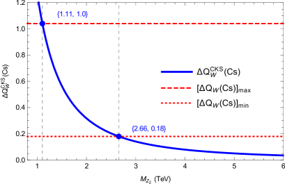
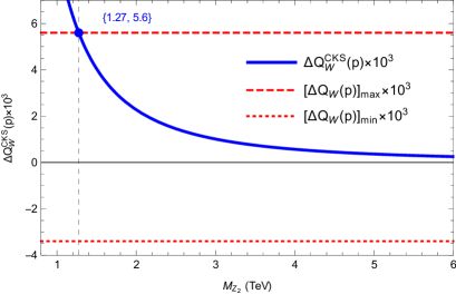
Figure 1: $\Delta Q_{W}^{\mathrm{CKS}}(Cs)$ and $\Delta Q_{W}^{\mathrm{CKS}}(p)$ as functions of the $Z_{2}$ mass

It follows that the allowed values of the $Z_{2}$ mass is $1.27\,\mathrm{TeV}\leq M_{Z_{2}}\leq 2.66$ TeV. This range is less restrict than that from the $\rho$ data Long:2018dun but it does not contradict it.

III Atomic parity violation in the 3 - 3 - 1 models for arbitrary beta

Let us briefly resume particle content of the model 3-3-1$\beta$ CarcamoHernandez:2005ka . Here the $\beta$ is defined in Eq. (1). The leptons lie in the $SU(3)_{L}$ triplet as follows

$$l_{aL}=\left(\nu_{a}\,,\hskip 8.5359pte_{a}\,,\hskip 8.5359ptE^{Q}_{a}\right)^{T}\sim\left(1,3,-\frac{1}{2}-\frac{\beta}{2\sqrt{3}}\right)\,,$$ (28)

where $a=1,2,3$ is generation index. This choice of lepton representation was called the model $F_{2}$ Buras:2014yna . On the other hand, there exist models (model $F_{1}$) that $l_{aL}$ are antitriplets, but it can be shown that they are always equivalent to some models with left-handed lepton triplets, in the sense that both have the same physics Martinez:2014lta ; Hue:2018dqf . Therefore, it is enough to focus on only the model $F_{2}$.

The chiral anomaly free requires the number of fermion triplets to be equal to that of fermion antitriplets. Therefore, in the model under consideration, one generation of quarks transforms as $SU(3)_{L}$ triplets and two others transform as $SU(3)_{L}$ antitriplets. However, it is free to assign to quarks, provided the model is anomaly free.

Here we adapt the notations in tables 1, 2, and 3 of Ref. CarcamoHernandez:2005ka . In particular, we consider the models containing just three Higgs triplets defined in Refs. CarcamoHernandez:2005ka ; Buras:2012dp , for example those given in Table 3 of Ref. CarcamoHernandez:2005ka . There are three different left-handed quark assignments, where the third, second or first left-handed quark family is assigned as triplet, three respective models reps. A, B, and C were introduced in Table 2 of Ref. CarcamoHernandez:2005ka . Recall that the right-handed fermions are $SU(3)_{L}$ singlets.

Note that the VEV of $\chi$ triplet provides masses of new particles, namely the exotic quarks and lepton as well as new gauge bosons: $Z^{\prime}$ and bilepton gauge bosons $X$ and $Y$. Remember that the bottom element of $\chi$ does not carry lepton number, while the similar elements of $\eta$ and $\rho$ triplets have lepton number equal to two. This means that only scalar components without lepton number can have VEV. In practice, to make the charged Higgs bosons having the integer value of electric charge, the parameter $\beta$ can take some special values only.

The masses and mixing of the neutral gauge bosons are presented in appendix B. The needed gauge couplings used to determine $Q_{W}$ are given in Table 5, where only two models A and C with different assignments of the first quark family are considered. The two models A and B have the same assignments of the first quark family, leading to the same APV result. Similar couplings were also given in Table 4 of Ref. CarcamoHernandez:2005ka , but they are different from ours by opposite signs, because of the difference choice of the phase of the $Z^{\prime}$ state.

Table 5: Vector and axial-vector coupling constants relevant for APV of the $3-3-1\,\beta$ model

Standard Model	The 3 - 3 - 1 model (rep. A)	The 3 - 3 - 1 model (rep. C)
$g_{A}(e)=-\frac{1}{2}$	$g^{\prime}_{A}(e)=\frac{1-(1+\sqrt{3}\beta)s^{2}_{W}}{2\sqrt{3}\sqrt{1-(1+\beta^{2})s^{2}_{W}}}$	$g^{\prime}_{A}(e)=\frac{1-(1+\sqrt{3}\beta)s^{2}_{W}}{2\sqrt{3}\sqrt{1-(1+\beta^{2})s^{2}_{W}}}$
$g_{V}(u)=\frac{1}{2}-\frac{4s_{W}^{2}}{3}$	$g^{\prime}_{V}(u)=\frac{-3+(3-5\sqrt{3}\beta)s_{W}^{2}}{6\sqrt{3}\sqrt{1-(1+\beta^{2})s_{W}^{2}}}$	$g^{\prime}_{V}(u)=\frac{3-(3+5\sqrt{3}\beta)s_{W}^{2}}{6\sqrt{3}\sqrt{1-(1+\beta^{2})s_{W}^{2}}}$
$g_{V}(d)=-\frac{1}{2}+\frac{2s_{W}^{2}}{3}$	$g^{\prime}_{V}(d)=\frac{-3+(3+\sqrt{3}\beta)s^{2}_{W}}{6\sqrt{3}\sqrt{1-(1+\beta^{2})s^{2}_{W}}}$	$g^{\prime}_{V}(d)=\frac{3-(3-\sqrt{3}\beta)s_{W}^{2}}{6\sqrt{3}\sqrt{1-(1+\beta^{2})s_{W}^{2}}}$

Now we turn back to our main intention, namely the deviation of the weak charge $\Delta Q_{W}^{331}(Cs)$ in the $3-3-1\,\beta$ model. The needed formula is also Eq. (24), will be applied to investigate the APV using the formula expressing the mixing $Z-Z^{\prime}$ in terms of the model parameter $\beta$ Buras:2014yna . The detailed steps to derive $\Delta Q_{W}^{331}(Cs)$ in the 3-3-1$\beta$ model are shown in appendix B. Contribution from $\Delta\rho$ will be neglected. The relevant $Z^{\prime}$ couplings are given in Table 5. With $M^{2}_{Z_{1}}\ll M^{2}_{Z_{2}}$, the $Z-Z^{\prime}$ mixing angle $\phi$ can be formulated as follows Buras:2014yna

$$s_{\phi}\simeq\tan\phi\simeq\frac{c_{W}^{2}}{3}\sqrt{f(\beta)}\left(3\beta t^{2}_{W}+\sqrt{3}c_{2v}\right)\left[\frac{M_{Z}^{2}}{M_{Z^{\prime}}^{2}}\right],$$ (29)

where

$$f(\beta)=\frac{1}{1-(1+\beta^{2})s_{W}^{2}},\quad c_{2v}\equiv\cos(2\beta_{v})=\frac{1-t^{2}_{v}}{1+t^{2}_{v}},\quad t_{v}\equiv\tan\beta_{v}\equiv\frac{v_{\rho}}{v_{\eta}}.$$ (30)

In the numerical calculation, we will use $\frac{M_{Z}^{2}}{M_{Z^{\prime}}^{2}}\simeq\frac{M_{Z_{1}}^{2}}{M_{Z_{2}}^{2}}$.

The parameter $t_{v}$ in Eq. (30) is constrained from the Yukawa couplings of the top quark in the third family, as in the well-known two Higgs doublet models (2HDM), for example see a review in Ref. Branco:2011iw . Depending on the model A (B, C), where left-handed top quarks are in triplets (anti-triplets), they get tree level mass mainly from the coupling to $\eta$ ($\rho$) CarcamoHernandez:2005ka . Especially, the top quark mass is $m_{t}\simeq\Gamma^{t}\times\frac{v_{\rho(\eta)}}{\sqrt{2}}$, where the Yukawa coupling should satisfy the perturbative limit: $|\Gamma^{t}|<\sqrt{4\pi}$, resulting in a lower bound $v_{\rho(\eta)}>\frac{m_{t}}{\sqrt{4\pi}}$. As a consequence, $t_{v}$ is constrained as

$$s_{v}=\frac{v_{\rho}}{\sqrt{v^{2}_{\rho}+v^{2}_{\eta}}}=\frac{gv_{\rho}}{2M_{W}}>\frac{g}{2M_{W}}\times\frac{m_{t}}{\sqrt{2\pi}}\simeq 0.28\Rightarrow t_{v}>t_{0}=\sqrt{\frac{1}{1-0.28^{2}}-1}\simeq 0.29$$ (31)

for top quark in anti-triplet (models B and C) and

$$c_{v}=\frac{v_{\eta}}{\sqrt{v^{2}_{\rho}+v^{2}_{\eta}}}=\frac{gv_{\eta}}{2M_{W}}>0.28\Rightarrow t_{v}<\sqrt{\frac{1}{0.28^{2}}-1}\simeq 3.43=t_{0}^{-1}$$ (32)

for top quark in triplet (model A). The constraint of $t_{v}$ in 3-3-1 models is similar to the 2HDMs Branco:2011iw . We will use $t_{v}\leq 3.4$ for model A and $t_{v}\geq 0.3$ for models B, C.

In the numerical investigation, we will look for allowed regions satisfying three constraints of the APV data of Cs, the PVES data of proton, and the perturbative limit of Yukawa coupling of the top quark. We will concentrate on the two models A and C. The allowed regions predicted by model B will be addressed based on the weak charges predicted by the model A and the condition  (31). Numerical results are presented as follows.

III.1 APV in the 3-3-1 model with $\beta=\pm\sqrt{3}$

III.1.1 The model with exotic leptons

The model we mention here is not the minimal 3-3-1 because the third components of lepton triplets are the exotic ones. The numerical results are illustrated in Fig. 2.

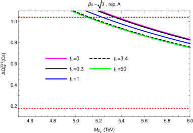
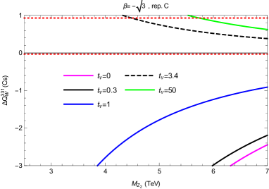
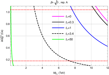
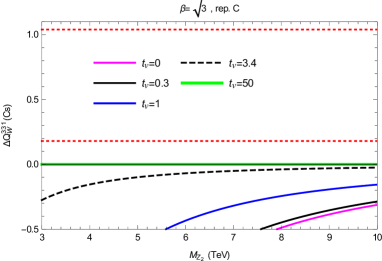
Figure 2: $\Delta Q_{W}^{331}(Cs)$ as a function of the $Z_{2}$ mass with $\beta=\pm\sqrt{3}$, predicted by rep. A (C) in the left (right) panel. The two red dotted lines present two lower and upper experimental bounds of $\Delta Q_{W}(Cs)$. We use $s^{2}_{W}(M_{Z_{2}})=0.246$ and $g=0.636$ Buras:2013dea

We used the numerical values of the $SU(2)_{L}$ gauge boson couplings and the Weinberg angle relating with $Z^{\prime}$ given in Ref. Buras:2013dea , where the renormalization group evolutions are taken into account. It also gives a consequence that the limit for perturbative calculations requires $M_{Z_{2}}<4$ TeV. In the models under consideration, the relation between $g_{X}$ and $g$ is determined by Eq. (48) from which the Landau pole arises at $s_{W}^{2}=1/(1+\beta^{2})$. For the $\beta=\pm\sqrt{3}$, the models lose their perturbative character at the scale around 4 TeV Ng:1992st ; Frampton:2002st ; Dias:2004dc ; Martinez:2006gb ; Buras:2013dea . We accept that the models will be ruled out if there are not any regions satisfying $M_{Z_{2}}\leq 4$ TeV.

From Fig.  2, we get the lowest value of $M_{Z_{2}}$ given in Table 6.

Table 6: Lower bounds of of $M_{Z_{2}}$[TeV] with $\beta=\pm\sqrt{3}$ from APV data of Cs

$\beta=-\sqrt{3}$	$\beta=+\sqrt{3}$
$t_{v}$ $0$ $0.3$ $1$ $3.4$ $50$ A 5.37 5.35 5.24 5.12 5.10 C Excl. Excl. Excl. 4.24 5.43	$t_{v}$ $0$ $0.3$ $1$ $3.4$ $50$ A 10.84 10.38 7.66 3.05 0.14 C Excl. Excl. Excl. Excl. Excl.

The following remarks are in order:

1. For $\beta=-\sqrt{3}$, the model rep. A always predicts the lowest allowed value of $M_{Z_{2}}$ around 5 TeV, where the perturbative property of the model is lost. The same conclusion for the model rep. C for $t_{v}=50$ or $t_{v}\leq 1$.

2. For $\beta=+\sqrt{3}$, the model rep. C is excluded for all values of $t_{v}$.

3. The value $t_{v}=3.4$ is survived for two models: rep. C with $\beta=-\sqrt{3}$ ($M_{Z_{2}}\geq 4.24$) and rep. A with $\beta=\sqrt{3}$ ($M_{Z_{2}}\geq 3.05$). Combining with the condition of the Yukawa coupling of top quark and PVES data of proton, the allowed regions are more strict, see Fig. 3.

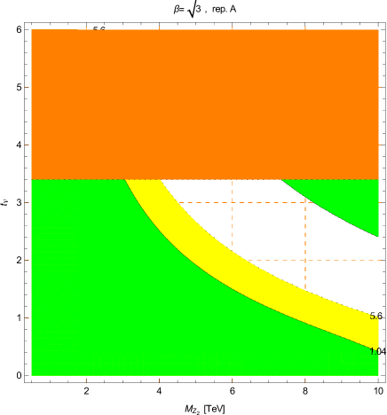
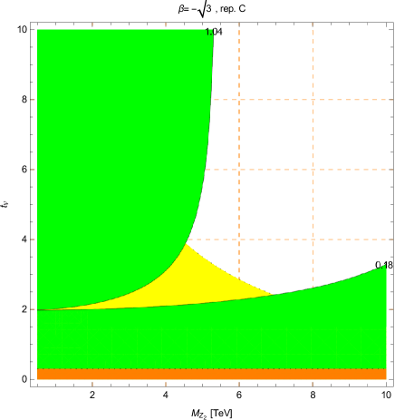
   Figure 3: Allowed regions in the plane $M_{Z_{2}}-t_{v}$ predicted by rep. A (C) with $\beta=\sqrt{3}$ ($\beta=-\sqrt{3}$), where the orange region is excluded by $t_{v}\leq 3.4$ ($t_{v}\geq 0.3$). The green and yellow regions are excluded by the APV data of Cs and PVES data of the proton, respectively.

   The $M_{Z_{2}}$ values must satisfy $M_{Z_{2}}\geq 4$ TeV for model rep. A and $M_{Z_{2}}\geq 4.5$ TeV for model rep. C. Hence the lower bounds from combined data are more constrained than those obtained from the data of APV of Cs alone.

III.1.2 The minimal 3-3-1 model

Apart from the case of $\beta=-\sqrt{3}$ mentioned above, another model with $\beta=-\sqrt{3}$ but no new charged lepton, i.e. the third components of the lepton triplets are conjugations of right-handed SM charged leptons, is well known as the minimal 3-3-1 model (M331). The gauge couplings relevant to the APV are given in table 7.

Table 7: Vector and axial-vector coupling constants relevant for APV M331 models

Standard Model	rep. A	rep. C
$g_{A}(e)=-\frac{1}{2}$	$g^{\prime}_{A}(e)=-\frac{\sqrt{1-4s_{W}^{2}}}{2\sqrt{3}}$	$g^{\prime}_{A}(e)=-\frac{\sqrt{1-4s_{W}^{2}}}{2\sqrt{3}}$
$g_{V}(u)=\frac{1}{2}-\frac{4s_{W}^{2}}{3}$	$g^{\prime}_{V}(u)=\frac{-1+6s_{W}^{2}}{2\sqrt{3}\sqrt{1-4s_{W}^{2}}}$	$g^{\prime}_{V}(u)=\frac{1+4s_{W}^{2}}{2\sqrt{3}\sqrt{1-4s_{W}^{2}}}$
$g_{V}(d)=-\frac{1}{2}+\frac{2s_{W}^{2}}{3}$	$g^{\prime}_{V}(d)=-\frac{1}{2\sqrt{3}\sqrt{1-4s_{W}^{2}}}$	$g^{\prime}_{V}(d)=\frac{1-2s_{W}^{2}}{2\sqrt{3}\sqrt{1-4s_{W}^{2}}}$

The numerical results are illustrated in Fig. 4.

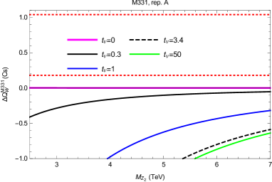
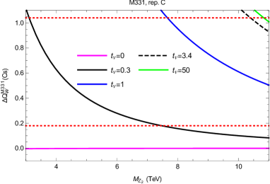
Figure 4: $\Delta Q_{W}^{\mathrm{M331}}(Cs)$ as a function of the $Z_{2}$ mass, predicted by the M331 model with the case of rep. A (C) in the left (right) panel. We have used $s^{2}_{W}(M_{Z_{2}})=0.246$ and $g=0.636$ Buras:2013dea

It can be seen that all curves are out of the allowed range given by experiment in the framework of rep. A. In contrast, there still exist allowed $M_{Z_{2}}$ values in the rep. C. Furthermore, small allowed $M_{Z_{2}}$ corresponds to small $t_{v}$. Some specific limits are summarized in Table 8.

Table 8: Allowed range of $M_{Z_{2}}$ for M331

$t_{v}$	$0$	$0.3$	$1$	$3.4$	$50$
A	excl.	excl.	excl.	excl.	excl.
C	excl.	[3.11, 7.47]	[7.66, 18.41]	[10.40, 24.99]	[10.83, 26.04]

We see that the data on APV of Cesium excludes the M331 model with rep. A, but still allows rep. C with some small $t_{v}$, for example $m_{Z_{2}}\geq 3.11$ TeV with $t_{v}=0.3$. Combining with the conditions of $t_{v}\geq 0.3$ and the PVES data of proton will give a more strict lower bound $m_{Z_{2}}\geq 4$ TeV, see Fig. 5. The lower bound of $M_{Z_{2}}$ obtained from the PVES data of proton is more strict than the APV data of Cs.

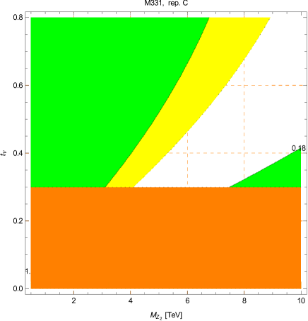
Figure 5: Allowed regions in the plane $M_{Z_{2}}-t_{v}$ predicted by rep. C of the M331. The orange region is excluded by $t_{v}\geq 0.3$. The green and yellow regions are excluded by the APV data of Cs and PVES data of the proton, respectively.

III.2 APV in the 3-3-1 model with $\beta=\pm\frac{1}{\sqrt{3}}$

Regarding the couplings of $Z^{\prime}$ at $M_{Z^{\prime}}=\mathcal{O}(1)$ TeV, we will use $g(M_{Z_{2}})=0.633$, $s^{2}_{W}(M_{Z_{2}})=0.249$ for $\beta=0,\pm\frac{1}{\sqrt{3}},\pm\frac{2}{\sqrt{3}}$ Buras:2013dea ; Buras:2016dxz ; Buras:2014yna . The numerical results obtained from APV of Cesium are shown in Fig. 6.

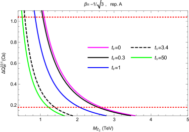
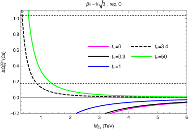
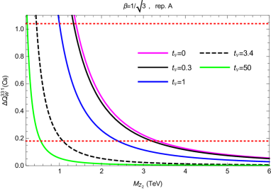
Figure 6: $\Delta Q_{W}^{331}(Cs)$ as a function of the $Z_{2}$ mass with $\beta=\pm\frac{1}{\sqrt{3}}$, predicted by rep. A (C) in the left (right) panel.

Some limits for $\beta=\pm\frac{1}{\sqrt{3}}$ are explicitly presented in Table 9.

Table 9: Allowed range of $M_{Z_{2}}$[TeV] for $\beta=\pm\frac{1}{\sqrt{3}}$

$\beta=-\frac{1}{\sqrt{3}}$	$t_{v}$ $0$ $0.3$ $1$ $3.4$ $50$ A [1.11, 2.66] [1.06, 2.57] [0.86, 2.07] [0.58, 1.39] [0.51, 1.23] C Excl. Excl. Excl. [0.35, 0.85] [0.57, 1.37]
$\beta=+\frac{1}{\sqrt{3}}$	A [1.39, 3.34] [1.33, 3.20] [1.00, 2.39] [0.45, 1.08] [0.23, 0.55] C Excl. Excl. Excl. Excl. [0.29, 0.70]

One gets the following results

1. For both $\beta=\pm\frac{1}{\sqrt{3}}$, the model rep. A survives with all $t_{v}$. The allowed values of $M_{Z_{2}}$ decrease with increasing $t_{v}$.

2. The model C survives with only large $t_{v}$ and small $M_{Z_{2}}\leq 1.5$ TeV.

III.3 APV in the 3-3-1 model with $\beta=0$

The 3-3-1 model with $\beta=0$ has been recently constructed in Ref. Hue:2015mna . The numerical results are shown in the Fig. 7.

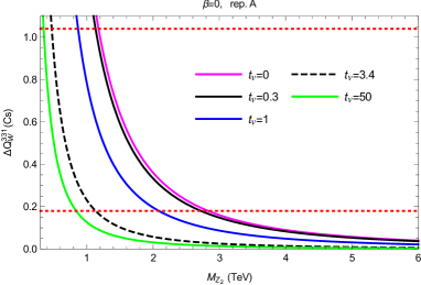
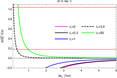
Figure 7: $\Delta Q_{W}^{331}(Cs)$ as a function of the $Z_{2}$ mass with $\beta=0$, predicted by rep. A (C) in the left (right) panel.

Result is summarized in Table 10.

Table 10: Allowed range of $M_{Z_{2}}$ for $\beta=0$

$t_{v}$	$0$	$0.3$	$1$	$3.4$	$50$
A	[1.18, 2.83]	[1.13, 2.72]	[0.87, 2.09]	[0.47, 1.13]	[0.35, 0.84]
C	excluded	excluded	excluded	[0.14, 0.33]	[0.41, 0.98]

We see the similarity to the cases $\beta=\pm\frac{1}{\sqrt{3}}$. These models predict a rather light $M_{Z_{2}}$, which was mentioned previously in other models Komachenko:1989qn ; Boucenna:2016qad ; Hue:2016nya ; He:2017bft . The difference is that the allowed ranges of $M_{Z_{2}}$ drift increasingly for $\beta$ changing from $-\frac{1}{\sqrt{3}}$ to $\frac{1}{\sqrt{3}}$.

There are some common properties for model rep. A, that we can see from all the above plots. Namely, the lower bounds of $M_{Z_{2}}$ involved with the APV of Cs are always increased corresponding to the decreasing $t_{v}$. As a result, an illustration of the allowed regions is shown in Fig. 8 for $\beta=0$.

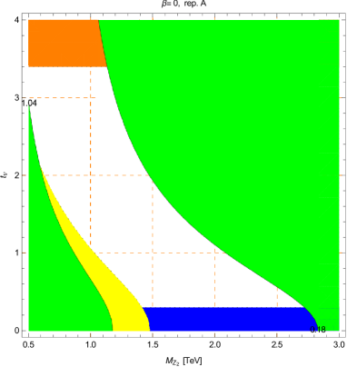
Figure 8: Allowed regions in the plane $M_{Z_{2}}-t_{v}$, predicted by rep. A with $\beta=0$. The orange, green and yellow regions are excluded by the condition $t_{v}\leq 3.4$, the APV data of Cs and the PVES data of the proton, respectively. The blue region is excluded by the condition $t_{v}\geq 0.3$.

Hence, perturbative condition $t_{v}\leq 3.4$ excludes regions of small $M_{Z_{2}}$. In the region with small $t_{v}\rightarrow 0$, the PVES data of the proton gives more strict lower bounds than the APV data of Cesium, see again Fig. 8. The largest allowed values of $M_{Z_{2}}$ is around 2.8 TeV. It increases to 4.65 TeV for $\beta=\frac{2}{\sqrt{3}}$.

Regarding to model rep. B, which has the same results of APV, but the allowed regions satisfy $t_{v}>0.3$, which can be seen in Fig. 8. The model B excludes regions containing large $M_{Z_{2}}$.

Illustrations for allowed regions predicted by model rep. C with $\beta=0,-\frac{1}{\sqrt{3}}$ are shown in Figs. 9.

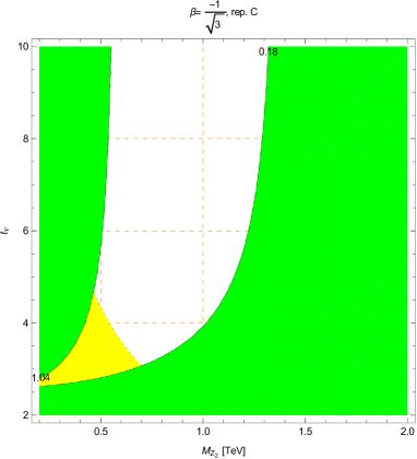
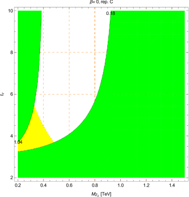
Figure 9: Allowed regions in the plane $M_{Z_{2}}-t_{v}$, predicted by rep.C. The green and yellow regions are excluded by the APV data of Cs and PVES data of the proton, respectively.

The PVES data of the proton excludes small $m_{Z_{2}}$ and $t_{v}$, which is more strict that the pertubative limit of top quark coupling. The allowed regions predict only small values $M_{Z_{2}}<1.5$ TeV. For other $\beta$ satisfying $|\beta|<\sqrt{3}$, the situations are similar to the mentioned illustrations, but the upper bounds of $M_{Z_{2}}$ may reach larger value of $2.5$ TeV.

IV Conclusions

The effects of the weak charges of Cesium and the proton on the parameter spaces of 3-3-1 models are discussed under the current experimental APV and PVES data and the perturbative limit of the Yukawa coupling of the top quark. Within a recently proposed 3-3-1 CKS, we get the lowest value of $M_{Z_{2}}$ to be 1.27 TeV. This limit is slightly lower than that concerned from the LHC searches, $B$ decays or $\rho$ parameter data.

We have also performed studies for the other versions of the 3-3-1 models with three Higgs triplets. Here are the main conclusions:

• $\beta=\pm\sqrt{3}$, the regions with $M_{Z_{2}}<4$ TeV are excluded in the frameworks of all models reps. A, C and M331. They are ruled out when the perturbative calculation limit are required, where the Landau pole of the models happens at the scale around 4 TeV. The APV data of Cesium alone rules out only three cases of the model C with $\beta=-\sqrt{3}$, the model rep. A with $\beta=\sqrt{3}$, and the M331 rep. A. Other cases are ruled out based on the PVES data of proton and top quark couplings limit.

• For $|\beta|<\sqrt{3}$, for example $\beta=0,\pm\frac{1}{\sqrt{3}}$, the allowed regions are affected significantly by the PVES data of proton, namely it results in the lower bounds of $M_{Z_{2}}$ more strict than those obtain from the APV data of Cesium. This point was not mentioned previously.

• For $\beta=0,\pm\frac{1}{\sqrt{3}}$, the model rep. C favors the regions with only small $M_{Z_{2}}<1.5$ TeV.

• For $\beta=\pm\frac{1}{\sqrt{3}}$, the model reps. A gives larger allowed values of $M_{Z_{2}}$. This model will not be ruled out by other constraints from LHC, where $M_{Z_{2}}\geq 2.5$ TeV with assumption that $Z_{2}$ does not decay to heavy fermions Richard:2013xfa ; Salazar:2015gxa , or all heavy fermion masses are 1 TeV Coutinho:2013lta . A reasonable lower bound were acceptable in literature $M_{Z_{2}}\geq 1$ TeV Buras:2013dea ; Hue:2017lak .

• The model rep. B also survives, although the perturbative limit of the Yukawa couplings of the top quark gives constraints on the allowed regions with large $M_{Z_{2}}$.

From our discussion, we emphasize that the information of PVES data of proton and the pertubative limit of top quark Yukawa couplings are as important as that obtained from the APV of Cesium, therefore all of them should be discussed simultaneously to constrain the parameter space of the 3-3-1 models. The numerical calculations have also shown that the allowed regions predicted by the two models reps. B and C disfavor the large $M_{Z_{2}}$ hence they may be ruled out by future constraints from colliders such as LHC, especially the model rep. C. While the model rep. A may still be survived, resulting in that the heaviest quark family must treat differently from the remaining. Furthermore, our work concerns that the improved weak charge data from the future experiments will be important to decide which quark family in realistic 3-3-1 models should be assigned differently from the two remaining families.

The recent data of APV and PVES is consistent with the data on the mass difference of neutral meson Long:1999ij in the sense that the third family should be treated differently from the first twos. This also gives a reason why the top quark is so heavy.

Appendix A Derivation of the weak charge expression in the models with extra neutral gauge boson

Nowadays, a lot of beyond Standard Models contain extra neutral gauge bosons associated with new diagonal generators such as $T_{8},T_{15}$ or extra generators of the new $U(1)_{N}$ groups. The above mentioned neutral gauge bosons will give contribution to the atomic parity violation. So we will provide a detailed analysis of the APV in the light of extra gauge bosons.

Some authors use the notations with different coefficients and signs associated with axial part ($\gamma_{5}$). Here we point out the relation among the notations.

A.1 Notations

For convenience to apply the results into our calculations, we review here more detailed steps to derive analytic formulas of $\Delta Q_{W}(^{A}_{Z}X)$. However, we firstly consider the case with just one extra neutral gauge boson $Z^{\prime}$. After some steps of diagonalization in neutral gauge boson sector, we come to two states $Z$ and $Z^{\prime}$ with Lagrangian (7). It is emphasized that the $Z$ and $Z^{\prime}$ are mixed and the physical states are a result of the last step of diagonalization which is discussed latter. In conventional way, the $Z$ and $Z^{\prime}$ are mixing with an angle $\phi$; and the consequence is a pair of the physical bosons $Z_{1}$ and $Z_{2}$. Relations between the notations in Eq. (7) and those mentioned in Ref. Altarelli:1991ci are

$$g_{V}(f)=2v_{f}\,,\hskip 8.5359ptg_{A}(f)=-2a(f)\,,\hskip 8.5359ptg^{\prime}_{V}(f)=2v^{\prime}_{f}\,,\hskip 8.5359ptg^{\prime}_{A}(f)=-2a^{\prime}(f)\,.$$ (33)

We will base on the approach to derive the deviation comparing with the results given by G. Altarelli et al. Altarelli:1991ci . The equivalence of the neutral gauge boson states between our notation and those in Ref. Altarelli:1991ci are (33) and

$$(Z,Z^{\prime})\equiv(Z_{0},\,Z^{\prime}_{0}),\quad(Z_{1},Z_{2})\equiv(Z,Z^{\prime}),\quad\xi_{0}\equiv\phi,\quad\tilde{g}=g^{\prime}=gt_{W}.$$

The mixing matrix $O$ relating two base of neutral gauge bosons are:

$$O=\begin{pmatrix}c_{\xi_{0}}&-s_{\xi_{0}}\\ s_{\xi_{0}}&c_{\xi_{0}}\end{pmatrix}\equiv\begin{pmatrix}c_{\phi}&-s_{\phi}\\ s_{\phi}&c_{\phi}\end{pmatrix},$$ (34)

which give $(Z_{1},Z_{2})^{T}=O(Z,Z^{\prime})^{T}$. We will use our notations in the following calculations.

Lagrangian containing gauge couplings of neutral gauge bosons in the basis $(Z,\,Z^{\prime})$ is

$$\mathcal{L}^{\mathrm{BSM}}_{Vff} =J_{\mu}Z^{\mu}+J^{\prime}_{\mu}Z^{\prime}_{\mu}$$

$$\equiv\frac{g}{2c_{W}}\sum_{f}\overline{f}\gamma^{\mu}[g_{V}(f)-\gamma_{5}g_{A}(f)]fZ_{\mu}+\frac{g}{2c_{W}}\sum_{f}\overline{f}\gamma^{\mu}[g^{\prime}_{V}(f)-\gamma_{5}g^{\prime}_{A}(f)]fZ^{\prime}_{\mu}\,.$$ (35)

On the other hand, in terms of physical neutral gauge boson mediations $Z_{1}$ and $Z_{2}$, this Lagrangian can be written as follows

$$\mathcal{L}^{\mathrm{BSM}}_{Vff} =\frac{g}{2c_{W}}\sum_{f}\overline{f}\gamma^{\mu}[g^{(1)}_{V}(f)-\gamma^{5}g^{(1)}_{A}(f)]fZ_{1\mu}+\frac{g}{2c_{W}}\sum_{f}\overline{f}\gamma^{\mu}[g^{(2)}_{V}(f)-\gamma^{5}g^{(2)}_{A}(f)]fZ_{2\mu},$$ (36)

where the couplings $g^{(1)}_{V}(f)$, $g^{(2)}_{V}(f)$, $g^{(1)}_{A}(f)$ and $g^{(2)}_{A}(f)$ are gauge couplings of the physical states of neutral gauge boson, which will be determined as functions of $g_{V,A}(f)$ and $g^{\prime}_{V,A}(f)$. Eq. (36) gives the following effective Lagrangian for a quark $f=u,d$:

$$\mathcal{L}^{f}_{\mathrm{eff}} =\frac{g^{2}}{4c^{2}_{W}M^{2}_{Z_{1}}}(\bar{e}\gamma_{\mu}\gamma^{5}e)\left(\bar{f}\gamma^{\mu}f\right)\left(g^{(1)}_{A}(e)g^{(1)}_{V}(f)+g^{(2)}_{A}(e)g^{(2)}_{V}(f)\frac{M^{2}_{Z_{1}}}{M^{2}_{Z_{2}}}\right)$$

$$=+\frac{G_{F}}{\sqrt{2}}(\bar{e}\gamma_{\mu}\gamma^{5}e)\left(\bar{f}\gamma^{\mu}f\right)\times 2\rho\left(g^{(1)}_{A}(e)g^{(1)}_{V}(f)+g^{(2)}_{A}(e)g^{(2)}_{V}(f)\frac{M^{2}_{Z_{1}}}{M^{2}_{Z_{2}}}\right)$$

$$\equiv-\frac{G_{F}}{2\sqrt{2}}(\bar{e}\gamma_{\mu}\gamma^{5}e)\left(\bar{f}\gamma^{\mu}f\right)\times C^{BSM}_{1}(f),$$ (37)

where we have denoted

$$C^{\mathrm{BSM}}_{1}(f)\equiv-4\rho\left(g^{(1)}_{A}(e)g^{(1)}_{V}(f)+g^{(2)}_{A}(e)g^{(2)}_{V}(f)\frac{M^{2}_{Z_{1}}}{M^{2}_{Z_{2}}}\right).$$ (38)

The parameter $\rho$ is defined in Eq. (20). Then a nuclear atom ${}^{A}_{Z}X$ with $Z$ protons and $N=A-Z$ neutrons consisting of $(2Z+N)$ quarks $u$ and $Z+2N$ quark $d$ in the first family has a weak charge determined as follows Diener:2011jt

$$Q^{\mathrm{BSM}}_{W}(^{A}_{Z}X)=\left[(2Z+N)C^{\mathrm{BSM}}_{1}(u)+(Z+2N)C^{\mathrm{BSM}}_{1}(d)\right],$$ (39)

In the SM, it has only neutral boson $Z\equiv Z_{1}$ with mass $M_{Z}\equiv M_{Z_{1}}$, while $\frac{M^{2}_{Z_{1}}}{M^{2}_{Z_{2}}}=0$, $g^{(1)}_{V,A}(f)=g_{V,A}(f)$ with $f=e,u,d$. It can be derived that $\rho=1$ and $C^{\mathrm{SM}}_{1}(f)\equiv-4\,g_{A}(e)g_{V}(f)$, resulting to the popular value APV of ${}^{133}_{55}Cs$ used to compare with experiments, namely

$$Q^{\mathrm{SM}}_{W}(^{133}_{55}Cs)=-73.8684.$$ (40)

The latest value of $Q^{\mathrm{SM}}_{W}(^{133}_{55}Cs)$ including other loop contributions is given in Ref. Tanabashi:2018oca .

From the $Z-Z^{\prime}$ mixing matrix $O$ given in (34), the states $Z$ and $Z^{\prime}$ are written as functions of $Z_{1,2}$. Inserting them into (A.1) then identifying the two Lagrangians (A.1) and (36), we obtain:

$$g^{(1)}_{A}(f) =c_{\phi}g_{A}(f)-s_{\phi}g^{\prime}_{A}(f),\quad g^{(1)}_{V}(f)=c_{\phi}g_{V}(f)-s_{\phi}g^{\prime}_{V}(f),$$

$$g^{(2)}_{A}(f) =s_{\phi}g_{A}(f)+c_{\phi}g^{\prime}_{A}(f),\quad g^{(2)}_{V}(f)=s_{\phi}g_{V}(f)+c_{\phi}g^{\prime}_{V}(f).$$ (41)

Now, $C^{\mathrm{BSM}}_{1}(f)$ is determined as follows:

$$C^{\mathrm{BSM}}_{1}(f) =-4\rho\left[\left(c^{2}_{\phi}+s^{2}_{\phi}\frac{M^{2}_{Z_{1}}}{M^{2}_{Z_{2}}}\right)g_{A}(e)g_{V}(f)\right.$$ (42)

$$-\left[g_{A}(e)g^{\prime}_{V}(f)+g^{\prime}_{A}(e)g_{V}(f)\right]\left(1-\frac{M^{2}_{Z_{1}}}{M^{2}_{Z_{2}}}\right)s_{\phi}c_{\phi}\left.+\left(s^{2}_{\phi}+c^{2}_{\phi}\frac{M^{2}_{Z_{1}}}{M^{2}_{Z_{2}}}\right)g^{\prime}_{A}(e)g^{\prime}_{V}(f)\right]\,.$$

To keep the approximation up to order of $O\left(\frac{M^{2}_{Z_{1}}}{M^{2}_{Z_{2}}}\right),$ we take $c_{\phi}\simeq 1,\;s^{2}_{\phi}\simeq 0$ in the first term of expression in (42) because $s_{\phi}\sim O\left(\frac{M^{2}_{Z_{1}}}{M^{2}_{Z_{2}}}\right)$. Hence, $g^{(1)}_{A}(e)g^{(1)}_{V}(f)\simeq g_{A}(e)g_{V}(f)-[g_{A}(e)g^{\prime}_{V}(f)+g^{\prime}_{A}(e)g_{V}(f)]s_{\phi}$. In contrast, the second term of (38) is simple, $g^{(2)}_{A}(e)g^{(2)}_{V}(f)\simeq g^{\prime}_{A}(e)g^{\prime}_{V}(f)$.

Thus

$$C^{\mathrm{BSM}}_{1}(f) =-4\rho\left[g_{A}(e)g_{V}(f)-\left[g_{A}(e)g^{\prime}_{V}(f)+g^{\prime}_{A}(e)g_{V}(f)\right]s_{\phi}+\left(\frac{M^{2}_{Z_{1}}}{M^{2}_{Z_{2}}}\right)g^{\prime}_{A}(e)g^{\prime}_{V}(f)\right]$$

$$+{\cal O}\left(\frac{M^{4}_{Z_{1}}}{M^{4}_{Z_{2}}}\right)\,.$$ (43)

Let us now deal with a derivation of the weak charge

$$\Delta Q^{\mathrm{BSM}}_{W}(^{A}_{Z}X) = Q^{\mathrm{BSM}}_{W}(^{A}_{Z}X)-Q^{\mathrm{SM}}_{W}(^{A}_{Z}X)$$ (44)

$$=-4\left\{\left(\frac{N-Z}{4}+Zs_{W}^{2}\right)\rho-\frac{N-Z}{4}+Zs_{W}^{2}\right.$$

$$-s_{\phi}\left((2Z+N)\left[g_{A}(e)g^{\prime}_{V}(u)+g^{\prime}_{A}(e)g_{V}(u)\right]\right.$$

$$+\left.(Z+2N)\left[g_{A}(e)g^{\prime}_{V}(d)+g^{\prime}_{A}(e)g_{V}(d)\right]\right)$$

$$\left.+\left(\frac{M_{Z_{1}}^{2}}{M^{2}_{Z_{2}}}\right)[(2Z+N)g^{\prime}_{A}(e)g^{\prime}_{V}(u)+(Z+2N)g^{\prime}_{A}(e)g^{\prime}_{V}(d)]\right\}$$

$$+{\cal O}\left(\frac{M^{4}_{Z_{1}}}{M^{4}_{Z_{2}}}\right),$$

where we have used the SM couplings of the electron, quarks $u$ and $d$ given in Table 4 and $\rho s_{\phi}\simeq s_{\phi}\,,\rho\left(\frac{M_{Z_{1}}^{2}}{M^{2}_{Z_{2}}}\right)\simeq\left(\frac{M_{Z_{1}}^{2}}{M^{2}_{Z_{2}}}\right)$.

To continue, we check the shift of $\delta(s_{W}^{2})$ introduced in Ref. Altarelli:1991ci . Using the formula

$$s_{W}^{2}c^{2}_{W}=\frac{\mu^{2}}{\rho M_{Z}^{2}},\quad\mu\equiv\frac{\pi\alpha}{\sqrt{2}G_{F}},$$ (45)

where $\mu$ and $M_{Z}$ are fixed as experimental inputs. Defining $x=s_{W}^{2}$, with $c^{2}_{W}=1-x$, as a variable in the following intermediate steps, ones have

$$(x-x^{2})\rho =\mathrm{const}\rightarrow 0=\frac{\delta}{\delta\,x}[(x-x^{2})\rho]=(1-2x)\rho+(x-x^{2})\frac{\delta\rho}{\delta\,x}$$

$$\rightarrow \hskip 8.5359pt\delta(s_{W}^{2})=\delta\,x=-\frac{x-x^{2}}{(1-2x)\rho}\delta\rho\simeq-\frac{s_{W}^{2}c_{W}^{2}}{c_{2W}}\Delta\rho\,.$$ (46)

Here we have used that fact that $\rho=1+\Delta\rho$ with $\Delta\rho=\mathcal{O}\left(\frac{M^{2}_{Z_{1}}}{M^{2}_{Z_{2}}}\right)$. The result in Eq. (A.1) is consistent with Eq. (2.13) of Ref. Altarelli:1991ci , but slight different from the expression used in Refs. Altarelli:1990dt ; Altarelli:1996pr ; Buras:2014yna .

To compare with the SM, we have to derive the deviation of $s^{2}_{W}$ and $\rho$ from the ones of the SM, namely $\rho\,\rightarrow\,1+\Delta\rho$ and $s^{2}_{W}\rightarrow\,s^{2}_{W}+\delta(s^{2}_{W})$, where $\delta\,(s^{2}_{W})$ is given in (A.1).

Applying the above procedure, we have

$$\Delta Q^{\mathrm{BSM}}_{W}(^{A}_{Z}X)=(Z-N)(1+\Delta\rho)-4Z[s_{W}^{2}(1+\Delta\rho)-\frac{s_{W}^{2}c_{W}^{2}}{c_{2W}}\Delta\rho]-Z-N-4Zs_{W}^{2}$$

$$+4s_{\phi}\left\{(2Z+N)\left[g_{A}(e)g^{\prime}_{V}(u)+g^{\prime}_{A}(e)g_{V}(u)\right]\right.$$

$$+\left.(Z+2N)\left[g_{A}(e)g^{\prime}_{V}(d)+g^{\prime}_{A}(e)g_{V}(d)\right]\right\}$$

$$-4\left(\frac{M_{Z_{1}}^{2}}{M^{2}_{Z_{2}}}\right)[(2Z+N)g^{\prime}_{A}(e)g^{\prime}_{V}(u)+(Z+2N)g^{\prime}_{A}(e)g^{\prime}_{V}(d)]+{\cal O}\left(\frac{M^{4}_{Z_{1}}}{M^{4}_{Z_{2}}}\right).$$ (47)

Substituting $N=A-Z$ into (47), we obtain the expression (I) for $\Delta Q^{\mathrm{BSM}}_{W}(^{A}_{Z}X)$. If the scale dependence of gauge couplings are taken into account, replacements need to be done in Eq. (7), namely $g\rightarrow g({M_{Z_{1,2}}})$ for couplings of $Z_{1,2}$, respectively. In addition, the factor in front of Eq. (A.1) is always $g^{2}(M_{Z_{1}})$, corresponding to the $M_{Z_{1}}$ scale. Hence, the $Z^{\prime}$ couplings in (47) should be replaced with $g^{\prime}_{A,V}(f)\rightarrow g^{\prime}_{A,V}(f)\times\frac{g(M_{Z_{2}})}{g(M_{Z_{1}})}$, resulting in Eq (I).

To conclude this section, we note that the above procedure can be easily extended for the Two Higgs Doublet Models with the addition of an Abelian gauge group  Campos:2017dgc , and the models with two or more extra gauge bosons, for instance the models based on the gauge group $\mbox{SU}(3)_{C}\times\mbox{SU}(4)_{L}\times\mbox{U}(1)_{X}$ Pisano:1994tf ; Long:2016lmj . In the framework of the 3-4-1 model, the APV has been considered in Ref. Nisperuza:2009xm .

Appendix B General discussions on recent 3-3-1 models

The APV can be considered in a more general class of 331 models with arbitrary parameter $\beta$ defined the electric charge of the model in Eq. (1). We consider here the popular class of 3-3-1 models with three Higgs triplets, namely the 3-3-1  $\beta$, where general analytic ingredient for determining APV such as the $Z-Z^{\prime}$ mixing $s_{\phi}$ and heavy neutral gauge boson are well-known CarcamoHernandez:2005ka ; Buras:2014yna . Furthermore, the formula of APV for these models was mentioned CarcamoHernandez:2005ka ; Martinez:2014lta , but it needs to be improved, at least because of the mixing angle and the scale dependence of the gauge couplings concerned in Ref. Buras:2014yna . In addition, many new models with $\beta\neq\pm\frac{1}{\sqrt{3}},\pm\sqrt{3}$ such as $\beta=0,\pm\frac{2}{\sqrt{3}}$ discussed recently should be paid attention to Buras:2014yna ; Buras:2012dp ; Hue:2015mna . The APV relating with these models will be discussed in the following.

Three Higgs triplets are defined the same as those given in Table 3 of Ref. CarcamoHernandez:2005ka , except that the VEVs of neutral components are denoted as those in Ref. Buras:2014yna for consistence with the definition of $t_{v}$ appearing in Eq. (30). The standard definitions of covariant derivatives were given in Ref. Buras:2012dp , which are consistent with Eq. (18) and

$$t\equiv\frac{g_{X}}{g}=\frac{\sqrt{6}s_{W}}{\sqrt{1-(1+\beta^{2})s_{W}^{2}}}.$$ (48)

The masses of the SM gauge bosons including $W^{\pm}_{\mu}=\frac{W^{1}_{\mu}\mp iW^{2}_{\mu}}{\sqrt{2}}$ and $Z_{\mu}$ are

$$M^{2}_{W}=\frac{g^{2}(v^{2}_{\rho}+v^{2}_{\eta})}{4},\quad M^{2}_{Z}=\frac{M_{W}^{2}}{c_{W}^{2}}.$$ (49)

After the breaking $SU(3)_{L}\otimes U(1)_{X}\rightarrow U(1)_{Q}$, the model consists of three neutral gauge bosons including one massless photon, a SM boson $Z_{\mu}$ and a new heavy $Z^{\prime}_{\mu}$ CarcamoHernandez:2005ka

$$A_{\mu} =s_{W}W^{3}_{\mu}+c_{W}\left(\beta t_{W}W^{8}_{\mu}+\sqrt{1-\beta^{2}t^{2}_{W}}B_{\mu}\right),$$

$$~{}Z_{\mu} =c_{W}W^{3}_{\mu}-s_{W}\left(\beta t_{W}W^{8}_{\mu}+\sqrt{1-\beta^{2}t^{2}_{W}}B_{\mu}\right),$$

$$~{}Z^{\prime}_{\mu} =\sqrt{1-\beta^{2}t^{2}_{W}}W^{8}_{\mu}-\beta\,t_{W}B_{\mu},$$ (50)

where the state $Z^{\prime}_{\mu}$ has an opposite sign with the choice in Ref. CarcamoHernandez:2005ka ; Buras:2014yna ; Martinez:2014lta in order to be consistent with the particular case of the 3-3-1 CKS model we mentioned above. In the limit $v_{\chi}\ll v_{\rho},v_{\eta}$, the $Z-Z^{\prime}$ mixing angle in Eq. (19) can be found as given in Eq. (29). We emphasize that this formula was introduced firstly in Ref. Buras:2014yna , which corrects the one in Ref. CarcamoHernandez:2005ka .

We note that our choice of the mixing matrix is

$$C_{ZZ^{\prime}}\equiv\begin{pmatrix}c_{\phi}&-s_{\phi}\\ s_{\phi}&c_{\phi}\end{pmatrix},$$ (51)

which defines the relation between two base of neutral gauge boson states: $(Z_{1},Z_{2})^{T}=C_{ZZ^{\prime}}(Z,Z^{\prime})^{T}$. The mixing angle $\phi$ in this definition is different from that in Refs. CarcamoHernandez:2005ka ; Buras:2014yna ; Martinez:2014lta by a minus sign. Combining with the state $Z^{\prime}$ defined in this work, the formula (29) determining $\phi$ was found to be consistent with Ref. Buras:2014yna . Based on this, the needed couplings can be calculated, as given in Table 5, where our notations coincide with those in Ref. CarcamoHernandez:2005ka . We can see that the mixing angle $\phi$ and couplings are consistent with the particular case of $\beta=0$ and $v_{\rho}=0$ we discussed above.

Now comparing with the result in table 4 of Ref. CarcamoHernandez:2005ka , we found an global opposite sign of $Z^{\prime}$ couplings, which can be removed by choosing the $Z^{\prime}$ state to have the same sign defined in Ref. CarcamoHernandez:2005ka . But a minus sign will also appear in the right-handed side of Eq. (29). In conclusion, both signs of $s_{\phi}$ and $Z^{\prime}$ couplings will be changed if the phase of the state $Z^{\prime}$ is changed, leading to the fact that the Eq. (I) is independent with the phase of $Z^{\prime}$.

Now we will pay attention to the ${}^{133}_{55}Cs$, where $\left(A-2.39782\times Z\right)\Delta\rho\simeq 1.12\Delta\rho=\mathcal{O}(10^{-4})\ll|\Delta Q(Cs)|$ following recent experimental results. Hence, in the framework of the 3-3-1  $\beta$ model, the expression for APV of $Cs$ is written as Eq. (25), based on Eq. (I), where the term depending on the $\rho$ parameter can be ignored. For $s_{\phi}$ given in Eq. (29), the respective $Z^{\prime}$ couplings are listed in Table 5.

References

- (1)
- (2) J. W. F. Valle and M. Singer, Phys. Rev. D 28 (1983) 540.
- (3) F. Pisano and V. Pleitez, Phys. Rev. D 46, 410 (1992) [hep-ph/9206242].
- (4) R. Foot, O. F. Hernandez, F. Pisano and V. Pleitez, Phys. Rev. D 47, 4158 (1993) [hep-ph/9207264].
- (5) P. H. Frampton, Phys. Rev. Lett. 69, 2889 (1992).
- (6) H. N. Long, Phys. Rev. D 54, 4691 (1996) [hep-ph/9607439].
- (7) H. N. Long, Phys. Rev. D 53, 437 (1996) [hep-ph/9504274].
- (8) R. Foot, H. N. Long and T. A. Tran, Phys. Rev. D 50, no. 1, R34 (1994) [hep-ph/9402243].
- (9) C. A. de Sousa Pires and O. P. Ravinez, Phys. Rev. D 58, 035008 (1998) [Phys. Rev. D 58, 35008 (1998)] [hep-ph/9803409].
- (10) P. V. Dong and H. N. Long, Int. J. Mod. Phys. A 21, 6677 (2006) [hep-ph/0507155].
- (11) J. C. Montero, V. Pleitez and O. Ravinez, Phys. Rev. D 60, 076003 (1999) [hep-ph/9811280].
- (12) J. C. Montero, C. C. Nishi, V. Pleitez, O. Ravinez and M. C. Rodriguez, Phys. Rev. D 73, 016003 (2006) [hep-ph/0511100].
- (13) P. B. Pal, Phys. Rev. D 52, 1659 (1995) [hep-ph/9411406].
- (14) A. G. Dias, V. Pleitez and M. D. Tonasse, Phys. Rev. D 67, 095008 (2003) [hep-ph/0211107].
- (15) A. G. Dias and V. Pleitez, Phys. Rev. D 69, 077702 (2004) [hep-ph/0308037].
- (16) A. G. Dias, C. A. de S. Pires and P. S. Rodrigues da Silva, Phys. Rev. D 68, 115009 (2003) [hep-ph/0309058].
- (17) A. E. Cárcamo Hernández, S. Kovalenko, H. N. Long and I. Schmidt, JHEP 1807 (2018) 144 [arXiv:1705.09169 [hep-ph]].
- (18) C. D. Froggatt and H. B. Nielsen, Nucl. Phys. B 147 (1979) 277.
- (19) A. E. Cárcamo Hernández, S. Kovalenko and I. Schmidt, JHEP 1702 (2017) 125 [arXiv:1611.09797 [hep-ph]].
- (20) K. Huitu and N. Koivunen, Phys. Rev. D 98 (2018) no.1, 011701 [arXiv:1706.09463 [hep-ph]].
- (21) H. N. Long, N. V. Hop, L. T. Hue, N. H. Thao and A. E. Cárcamo Hernández: Higgs and gauge boson phenomenology of the 3-3-1 model with CKS mechanism, arXiv:1810.00605 [hep-ph].
- (22) F. F. Freitas, C. A. de S. Pires and P. Vasconcelos, Phys. Rev. D 98 (2018) no.3, 035005 [arXiv:1805.09082 [hep-ph]].
- (23) M. Aaboud et al. [ATLAS Collaboration], JHEP 1710 (2017) 182 [arXiv:1707.02424 [hep-ex]].
- (24) M. Aaboud et al. [ATLAS Collaboration], JHEP 1801 (2018) 055 [arXiv:1709.07242 [hep-ex]].
- (25) A. M. Sirunyan et al. [CMS Collaboration], JHEP 1806 (2018) 120 [arXiv:1803.06292 [hep-ex]].
- (26) G. Aad et al. [ATLAS Collaboration], “Search for high-mass dilepton resonances using 139 fb-1 of collision data collected at 13 TeV with the ATLAS detector,” arXiv:1903.06248 [hep-ex].
- (27) G. Corcella, C. Corianò, A. Costantini and P. H. Frampton, Phys. Lett. B 785 (2018) 73 [arXiv:1806.04536 [hep-ph]].
- (28) S. C. Bennett and C. E. Wieman, Phys. Rev. Lett. 82 (1999) 2484 Erratum: [Phys. Rev. Lett. 82 (1999) 4153] Erratum: [Phys. Rev. Lett. 83 (1999) 889] [hep-ex/9903022].
- (29) C. Bouchiat and P. Fayet, Phys. Lett. B 608 (2005) 87 [hep-ph/0410260].
- (30) H. Davoudiasl, H. S. Lee and W. J. Marciano, Phys. Rev. Lett. 109 (2012) 031802 [arXiv:1205.2709 [hep-ph]].
- (31) J. L. Rosner, Phys. Rev. D 65 (2002) 073026 [hep-ph/0109239].
- (32) J. S. M. Ginges and V. V. Flambaum, Phys. Rept. 397 (2004) 63 [physics/0309054].
- (33) J. Guena, M. Lintz and M. A. Bouchiat, Mod. Phys. Lett. A 20 (2005) 375 [physics/0503143].
- (34) J. Erler, C. J. Horowitz, S. Mantry and P. A. Souder, Ann. Rev. Nucl. Part. Sci. 64 (2014) 269 [arXiv:1401.6199 [hep-ph]].
- (35) V. A. Dzuba, J. C. Berengut, V. V. Flambaum and B. Roberts, Phys. Rev. Lett. 109 (2012) 203003 [arXiv:1207.5864 [hep-ph]].
- (36) M. Tanabashi et al. [Particle Data Group], Phys. Rev. D 98 (2018) no.3, 030001.
- (37) J. Erler and S. Su, Prog. Part. Nucl. Phys. 71 (2013) 119 [arXiv:1303.5522 [hep-ph]].
- (38) P. Souder and K. D. Paschke, Front. Phys. (Beijing) 11 (2016) no.1, 111301. doi:10.1007/s11467-015-0482-0
- (39) D. Androíc et al. [Qweak Collaboration], Nature 557 (2018) no.7704, 207.
- (40) G. Altarelli, R. Casalbuoni, S. De Curtis, N. Di Bartolomeo, F. Feruglio and R. Gatto, Phys. Lett. B 261 (1991) 146.
- (41) H. N. Long and L. P. Trung, Phys. Lett. B 502 (2001) 63 [hep-ph/0010204].
- (42) A. E. Carcamo Hernandez, R. Martinez and F. Ochoa, Phys. Rev. D 73 (2006) 035007 [hep-ph/0510421].
- (43) D. A. Gutierrez, W. A. Ponce and L. A. Sanchez, Int. J. Mod. Phys. A 21 (2006) 2217 [hep-ph/0511057].
- (44) P. V. Dong, H. N. Long and D. T. Nhung, Phys. Lett. B 639 (2006) 527 [hep-ph/0604199].
- (45) J. C. Salazar, W. A. Ponce and D. A. Gutierrez, Phys. Rev. D 75 (2007) 075016 [hep-ph/0703300 [HEP-PH]].
- (46) R. Gauld, F. Goertz and U. Haisch, JHEP 1401 (2014) 069 [arXiv:1310.1082 [hep-ph]].
- (47) R. Martinez and F. Ochoa, Phys. Rev. D 90 (2014) no.1, 015028 [arXiv:1405.4566 [hep-ph]].
- (48) A. J. Buras, F. De Fazio and J. Girrbach, JHEP 1402 (2014) 112 [arXiv:1311.6729 [hep-ph]].
- (49) A. J. Buras, F. De Fazio and J. Girrbach-Noe, JHEP 1408 (2014) 039 [arXiv:1405.3850 [hep-ph]].
- (50) J. Beringer et al. [Particle Data Group], Phys. Rev. D 86 (2012) 010001.
- (51) R. Martinez and F. Ochoa, Eur. Phys. J. C 51, 701 (2007) [hep-ph/0606173].
- (52) F. Ochoa and R. Martinez, “Z-Z’ mixing in SU(3)(c) x SU(3)(L) x U(1)(X) models with beta arbitrary”, hep-ph/0508082.
- (53) D. Chang and H. N. Long, Phys. Rev. D 73, 053006 (2006) [hep-ph/0603098].
- (54) M. E. Peskin and T. Takeuchi, Phys. Rev. Lett. 65 (1990) 964.
- (55) H. N. Long and T. Inami, Phys. Rev. D 61, 075002 (2000) [hep-ph/9902475].
- (56) L. T. Hue and L. D. Ninh, Eur. Phys. J. C 79 (2019) no.3, 221 [arXiv:1812.07225 [hep-ph]].
- (57) A. J. Buras, F. De Fazio, J. Girrbach and M. V. Carlucci, JHEP 1302 (2013) 023 [arXiv:1211.1237 [hep-ph]].
- (58) G. C. Branco, P. M. Ferreira, L. Lavoura, M. N. Rebelo, M. Sher and J. P. Silva, Phys. Rept. 516 (2012) 1 [arXiv:1106.0034 [hep-ph]].
- (59) D. Ng, Phys. Rev. D 49 (1994) 4805 [hep-ph/9212284].
- (60) A. G. Dias, R. Martinez and V. Pleitez, Eur. Phys. J. C 39 (2005) 101 [hep-ph/0407141].
- (61) P. H. Frampton, Mod. Phys. Lett. A 18 (2003) 1377 [hep-ph/0208044].
- (62) A. J. Buras and F. De Fazio, JHEP 1608 (2016) 115 [arXiv:1604.02344 [hep-ph]].
- (63) L. T. Hue and L. D. Ninh, Mod. Phys. Lett. A 31 (2016) no.10, 1650062 [arXiv:1510.00302 [hep-ph]].
- (64) Y. Y. Komachenko and M. Y. Khlopov, Sov. J. Nucl. Phys. 51 (1990) 692 [Yad. Fiz. 51 (1990) 1081].
- (65) S. M. Boucenna, A. Celis, J. Fuentes-Martin, A. Vicente and J. Virto, JHEP 1612 (2016) 059
- (66) L. T. Hue, A. B. Arbuzov, N. T. K. Ngan and H. N. Long, Eur. Phys. J. C 77 (2017) no.5, 346 [arXiv:1611.06801 [hep-ph]].
- (67) X. G. He and G. Valencia, Phys. Lett. B 779 (2018) 52 [arXiv:1711.09525 [hep-ph]].
- (68) F. Richard, “A Z-prime interpretation of BdK*mu+mu- data and consequences for high energy colliders,” arXiv:1312.2467 [hep-ph].
- (69) C. Salazar, R. H. Benavides, W. A. Ponce and E. Rojas, JHEP 1507 (2015) 096 [arXiv:1503.03519 [hep-ph]].
- (70) Y. A. Coutinho, V. Salustino Guimarães and A. A. Nepomuceno, Phys. Rev. D 87 (2013) no.11, 115014 [arXiv:1304.7907 [hep-ph]].
- (71) L. T. Hue, L. D. Ninh, T. T. Thuc and N. T. T. Dat, Eur. Phys. J. C 78 (2018) no.2, 128 [arXiv:1708.09723 [hep-ph]].
- (72) H. N. Long and V. T. Van, J. Phys. G 25, 2319 (1999) [hep-ph/9909302].
- (73) R. Diener, S. Godfrey and I. Turan, Phys. Rev. D 86 (2012) 115017 [arXiv:1111.4566 [hep-ph]].
- (74) G. Altarelli, R. Casalbuoni, D. Dominici, F. Feruglio and R. Gatto, Nucl. Phys. B 342 (1990) 15.
- (75) G. Altarelli, N. Di Bartolomeo, F. Feruglio, R. Gatto and M. L. Mangano, Phys. Lett. B 375 (1996) 292 [hep-ph/9601324].
- (76) M. D. Campos, D. Cogollo, M. Lindner, T. Melo, F. S. Queiroz and W. Rodejohann, JHEP 1708 (2017) 092 [arXiv:1705.05388 [hep-ph]].
- (77) F. Pisano and V. Pleitez, Phys. Rev. D 51, 3865 (1995) [hep-ph/9401272].
- (78) H. N. Long, L. T. Hue and D. V. Loi, Phys. Rev. D 94, no. 1, 015007 (2016) [arXiv:1605.07835 [hep-ph]].
- (79) J. L. Nisperuza and L. A. Sanchez, Phys. Rev. D 80, 035003 (2009) [arXiv:0907.2754 [hep-ph]].