One-dimensional two-component fermions with contact even-wave repulsion and SU(2) breaking near-resonant odd-wave attraction

Abstract

We consider a one-dimensional (1D) two-component atomic Fermi gas with contact interaction in the even-wave channel (Yang-Gaudin model) and study the effect of an SU(2) symmetry breaking near-resonant odd-wave interaction within one of the components. Starting from the microscopic Hamiltonian, we derive an effective field theory for the spin degrees of freedom using the bosonization technique. It is shown that at a critical value of the odd-wave interaction there is a first-order phase transition from a phase with zero total spin and zero magnetization to the spin-segregated phase where the magnetization locally differs from zero.

I Introduction

Over the last decades there has been a tremendous progress in the field of ultracold atomic quantum gases Bloch2008 ; Guan2013 ; Massignan2014 . Unprecedented degree of precision, tunability, and control allows one to study an immense diversity of physical systems that are of great interest from the condensed matter physics perspective. Ultracold gases of atomic fermions that are in two internal states can be mapped onto spin-1/2 fermions treating the internal energy states as pseudospin states. These gases serve as an ideal platform for simulating a large variety of magnetically ordered phases, in particular, an itinerant ferromagnetic state.

Itinerant ferromagnetism of spin-1/2 fermions in condensed matter systems is a long-standing problem Vollhardt2001_Lohneysen2007 ; Moriya1984_85 ; Tasaki1998 . It has also been intensively studied in the context of ultracold quantum gases (see Ref. Massignan2014 for a review). It is believed that the Stoner criterion Stoner1933 (which requires a strong repulsion between different spin components) alone will not lead to the formation of an itinerant ferromagnetic state Pekker2011 ; Sanner2012 . Despite a vast amount of experimental Jo2009 ; Sanner2012 ; Scazza2017 ; Valtolina2017 ; Amico2018 and theoretical Pekker2011 ; theor ; Yang2004 ; Kozii2017 studies on itinerant ferromagnetism, many aspects, such as the character of the ferromagnetic phase transition remain disputable Massignan2014 . Recent experimental advances in time-resolved spectroscopic techniques Scazza2017 ; Amico2018 provide new prospects for studying itinerant ferromagnetism in ultracold quantum gases and renew the interest to this intriguing topic.

In the one-dimensional case, it has been realized long ago that the Stoner criterion is not valid. According to the Lieb-Mattis theorem Lieb1962 ; Aizenman1990 , in a one-dimensional two-component Fermi gas with a contact repulsive interaction between different spin species, the ferromagnetic state has a higher energy for any finite repulsion strength. In the limit of infinitely strong repulsion all spin configurations are degenerate Ogata1990 ; Shiba1991 . Recently, it has been shown that the itinerant ferromagnetic ground state can be realized in a 1D two-component Fermi gas with an infinite Jiang2016 or a very strong Yang2016 contact interspecies repulsion and an odd-wave attraction within one of the components. These proposals are very promising as they require regimes of the interactions that are reachable already with the present experimental facilities 40K . However, the regime of finite and moderate repulsion strength has not been investigated. It is the purpose of this paper to fill in this gap.

We use bosonization and renormalization group (RG) techniques to study an effective field theory for a one-dimensional two-component Fermi gas with a contact repulsion between different components and an odd-wave attractive interaction within one of the components. The contact repulsive interaction is assumed to be in the weak or intermediate regime and the odd-wave attraction in the near resonant regime (precise definitions will be given below). It is shown that at a critical value of the odd-wave interaction there is a first-order phase transition from a phase with zero total spin and zero magnetization to the spin-segregated phase where the magnetization locally differs from zero.

This paper is organized as follows. In Section II we specify the microscopic model and describe the interactions between the particles. In Section III we derive an effective field theory for the spin degrees of freedom using the bosonization technique. The resulting field theory is then studied using renormalization group analyzis in Section IV, and in Section V we derive the phase transition criterion. Finally, in Section VI we conclude.

II Interaction between particles and Hamiltonian of the system

We begin with a brief description of the model. Consider a two-component one-dimensional atomic Fermi gas in free space at zero temperature. The total Hamiltonian is $H=H_{0}+H_{\uparrow\downarrow}+H^{\prime}$, which includes the free part $H_{0}$ and two types of the interaction. The interaction between different (pseudo)spin species, $H_{\uparrow\downarrow}$, is assumed to be contact and repulsive, and it takes place in the even-wave scattering channel. The term $H^{\prime}$ describes the intraspecies attractive interaction in the odd-wave channel. Let us now discuss both interactions in detail.

II.1 Even-wave interaction

In the absence of the odd-wave interaction, the model reduces to the well-known Yang-Gaudin model with Hamiltonian $H_{\text{YG}}=H_{0}+H_{\uparrow\downarrow}$, which explicitly reads (we use units in which $\hbar=1$, unless specified otherwise):

$$H_{\text{YG}}=\int dx\Bigl{\{}-\frac{1}{2m}\sum_{j=\uparrow,\downarrow}\psi^{{\dagger}}_{j}\partial_{x}^{2}\psi_{j}+g\psi^{{\dagger}}_{\uparrow}\psi^{{\dagger}}_{\downarrow}\psi_{\downarrow}\psi_{\uparrow}\Bigr{\}}.$$ (1)

Here $\psi_{j}$ is the field operator for a fermion in the (pseudo)spin state $j=\uparrow,\downarrow$ and $g$ is the even-wave interaction coupling constant. The model is exactly solvable Gaudin1967 ; Yang1967 and it is well known that for any finite repulsion ($g>0$) the ground state has total spin $S=0$. In the limit of infinite repulsion strength $g\to+\infty$ all spin configurations are degenerate Ogata1990 . Thus, in agreement with the Lieb-Mattis theorem, the even-wave contact repulsion alone cannot lead to the ground state with nonzero total spin Lieb1962 ; Aizenman1990 . The situation changes if one takes into account the interaction in the odd-wave scattering channel. This interaction is momentum-dependent and the Lieb-Mattis theorem no longer applies.

II.2 Odd-wave interaction

For ultracold fermions the background odd-wave interaction is rather weak, since it is proportional to the square of the relative momentum of colliding particles. Nevertheless, the interaction strenght can be enhanced using a Feshbach resonance. Just like $p$-wave interaction in higher dimensions, odd-wave interaction in one dimension takes place in the spin-triplet state of colliding particles. However, under realistic conditions a Feshbach resonance is usually only present for one of the states out of the triplet. For example, in the case of ⁴⁰K atoms there is a $p$-wave resonance at magnetic field 198.8 G Jin2002 ; Regal2003 , and it is present only between two atoms in the $\left|F=9/2,m_{F}=-7/2\right>$ states. Therefore, in the presence of the Feshbach resonance the odd-wave interaction, typically, is not SU$(2)$-invariant.

The case of 1D spin-polarized fermions with resonant odd-wave interaction has been studied previously by means of the asymptotic Bethe ansatz Imambekov2010 . This approach relies on the knowledge of the two-body scattering phase shift (first derived in Ref. Pricoupenko2008 ) and does not require an explicit form of the Hamiltonian. In the two-component case that we are dealing with, the asymptotic Bethe ansatz becomes cumbersome due to the existence of both charge and spin excitations. For this reason, we proceed differently and take into account the resonant odd-wave interaction using the so-called two-channel model that accurately captures microscopic physics of the interaction. This model describes the Feshbach resonant interaction as an interconversion between pairs of fermionic atoms in the open channel and weakly bound bosonic dimers in the closed channel sWave2ch ; Gurarie2007 ; Prem2018 .

Thus, keeping in mind the absence of SU(2) symmetry, we now include an odd-wave interaction within one of the components, say, between spin-$\uparrow$ fermions. The corresponding two-channel Hamiltonian in the momentum representation reads Cui2016

$$H^{\prime}=\sum_{q}\left(\frac{q^{2}}{4m}+\nu\right)b^{{\dagger}}_{q}b_{q}$$ (2)

$$+\frac{\lambda}{\sqrt{L}}\sum_{k_{1},k_{2}}\frac{k_{1}-k_{2}}{2}\left[b^{{\dagger}}_{k_{1}+k_{2}}a_{k_{1},\uparrow}a_{k_{2},\uparrow}+\text{H.c.}\right].$$

Here $\hat{a}^{{\dagger}}_{k,\uparrow}$ is the fermionic creation operator of an (open channel) atom in the spin-$\uparrow$ state with mass $m$ and momentum $k$. The bosonic operator $\hat{b}^{{\dagger}}_{q}$ creates an odd-wave (closed channel) dimer of spin-$\uparrow$ atoms with mass $2m$ and a center of mass momentum $q$. We denote by $\lambda$ the atom-dimer interconversion strength and the bare detuning of a dimer by $\nu$. The latter is related to the dimer binding energy and can be tuned by an external magnetic field. The odd-wave interaction is momentum-dependent, and we introduce an ultraviolet momentum cutoff $\Lambda$, above which the interconversion strength $\lambda$ vanishes.

One can relate the bare parameters of the odd-wave interaction ($\lambda$ and $\nu$) to the physical scattering parameters by calculating diagrammatically the two-body scattering amplitude Cui2016 :

$$f(k)=\frac{-ik}{-\hbar^{2}\nu/m\lambda^{2}+2\Lambda/\pi+(\hbar^{4}/m^{2}\lambda^{2})k^{2}+ik},$$ (3)

where we restored $\hbar$ for clarity. Comparing Eq. (3) with the general form of the 1D odd-wave scattering amplitude at low collisional energy, $f(k)=-ik/[1/l_{p}+\xi_{p}k^{2}+ik]$, where $l_{p}$ is the 1D odd-wave scattering length and $\xi_{p}$ is the 1D effective range Pricoupenko2008 , we find:

$$l_{p}=-\,\frac{m\lambda^{2}}{\hbar^{2}}\frac{1}{\nu-2m\lambda^{2}\Lambda/\pi\hbar^{2}},\qquad\xi_{p}=\frac{\hbar^{4}}{m^{2}\lambda^{2}}.$$ (4)

We see that the momentum cutoff $\Lambda$ simply results in the renormalization of the bare detuning $\nu$, similarly to the case of $s$-wave Feshbach resonant scattering in 3D Gurarie2007 ; Levinsen2011 .

Attractive odd-wave interaction corresponds to $l_{p}<0$. It follows from Eq. (4) that in this case the bare detuning is necessarily positive and satisfies the condition

$$\nu>\frac{2\Lambda}{\pi}\frac{\hbar^{2}}{m\xi_{p}}.$$ (5)

Let us estimate the right hand side of inequality (5). In the quasi-1D regime obtained by a tight harmonic confinement in transverse directions with frequency $\omega_{\perp}$ the 1D effective range can be written as $\xi_{p}=\alpha_{1}a_{\perp}^{2}/3$, where $a_{\perp}=\sqrt{\hbar/m\omega_{\perp}}$ is the oscillator length and $\alpha_{1}$ is the 3D effective range Pricoupenko2008 . Eq. (5) then becomes $\nu>(6\Lambda/\pi\alpha_{1})\hbar\omega_{\perp}$, where the right hand side can now be easily estimated. Indeed, the 1D regime requires that $\hbar\omega_{\perp}\gg E_{F}$ and $a_{\perp}\gg R_{e}$, where $E_{F}$ is the Fermi energy and $R_{e}$ is the effective radius of the actual interaction potential between atoms. The first condition gives $1/a_{\perp}\gg k_{F}$, and hence we may put the momentum cutoff to be $\Lambda\sim 1/a_{\perp}$. Then, the second condition implies that the ratio $\Lambda/\alpha_{1}\ll 1$, since the 3D effective range $\alpha_{1}$ is typically of the order of $R_{e}^{-1}$. Therefore, for attractive interactions the lower bound of the bare detuning $\nu$ is of the order of $E_{F}$. As $\nu$ approaches this lower bound one enters the regime of resonant interactions, where $|l_{p}|$ is very large. On the contrary, in the off-resonant regime, where $|l_{p}|$ is small, the bare detuning is $\nu\gg E_{F}$. Then, from Eq. (4) we have $l_{p}\approx-m\lambda^{2}/\hbar^{2}\nu$.

II.3 Effective odd-wave interaction

In this subsection we integrate out the closed channel bosonic dimers and obtain an effective action for the fermionic fields. The Euclidean action corresponding to Hamiltonian (2) is

$$S^{\prime}=\int d\tau dx\left\{\bar{\chi}\left(\partial_{\tau}-\frac{1}{4m}\partial^{2}_{x}+\nu\right)\chi+\lambda\Bigl{(}\bar{\chi}{\cal O}+\bar{\cal O}\chi\Bigr{)}\right\},$$ (6)

where $\tau=it$ is the imaginary time, $\chi$ and $\bar{\chi}$ are bosonic complex fields, and we defined

$${\cal O}(x,\tau)=\psi_{\uparrow}\bigl{(}i\partial_{x}\psi_{\uparrow}\bigr{)}-\bigl{(}i\partial_{x}\psi_{\uparrow}\bigr{)}\psi_{\uparrow}.$$ (7)

Integrating out the bosonic fields we obtain an effective action that contains only the fermionic fields:

$$S^{\prime}_{\text{eff}}=\lambda^{2}\int d{\bf 1}d{\bf 2}\;\bar{\cal O}({\bf 1}){\cal G}({\bf 1}-{\bf 2}){\cal O}({\bf 2}),$$ (8)

where ${\bf 1}\equiv(x,\tau)$ and ${\bf 2}\equiv(x^{\prime},\tau^{\prime})$. The bosonic propagator ${\cal G}(x,\tau)$ satisfies the equation

$$\left(-\partial_{\tau}+\frac{1}{4m}\partial^{2}_{x}-\nu\right){\cal G}(x,\tau)=\delta(x)\delta(\tau)$$ (9)

and at zero temperature it reads

$${\cal G}(x,\tau)=-\theta(\tau)\sqrt{\frac{m}{\pi\tau}}\exp\left\{-\frac{mx^{2}}{\tau}-\nu\tau\right\}.$$ (10)

We see that, since $\nu$ is large and positive, the propagator is strongly localized in the vicinity of $x=\tau=0$.

III Bosonization Procedure

III.1 Notations

We now focus on the low-energy scattering near the Fermi points. In this subsection we briefly discuss the notations that we are going to use. The fermionic field is decomposed as

$$\psi_{j}(x,\tau)\approx e^{ik_{F}x}R_{j}(x,\tau)+e^{-ik_{F}x}L_{j}(x,\tau),$$ (11)

where $j=\uparrow,\downarrow$ is the spin index and $k_{F}=\pi n/2$ is the single-component Fermi momentum, with $n$ being the total fermionic density. For the slow fields $R_{j}$, $L_{j}$ we employ the bosonization identity in the following form:

$$R_{j}(x,\tau) =\frac{1}{\sqrt{2\pi a}}\,e^{-i\sqrt{\pi}\left\{\Phi_{j}(x,\tau)+\Theta_{j}(x,\tau)\right\}},$$ (12)

$$L_{j}(x,\tau) =\frac{1}{\sqrt{2\pi a}}e^{i\sqrt{\pi}\left\{\Phi_{j}(x,\tau)-\Theta_{j}(x,\tau)\right\}},$$

where $a$ is the short distance cut-off. In equation (12), $\Phi_{j}$ is the compact bosonic field and $\Theta_{j}$ is the corresponding dual field. The latter is defined as

$$\Theta_{j}(x,\tau)=-\int_{-\infty}^{x}dy\,\Pi_{j}(y,\tau),$$ (13)

where $\Pi_{j}$ is the canonical momentum conjugated to the field $\Phi_{j}$. Thus, one has the following equal time commutation relations $\left[\Phi_{j}(x,\tau),-\partial_{x^{\prime}}\Theta_{j}(x^{\prime},\tau)\right]=i\delta(x-x^{\prime})$. For later purposes we also introduce a canonical momentum $\pi_{j}$ conjugated to the dual field $\Theta_{j}$. It is defined as

$$\pi_{j}(x,\tau)=-\int_{-\infty}^{x}dy\,\Theta_{j}(y,\tau)$$ (14)

and satisfies the commutation relations $\left[\Theta_{j}(x,\tau),-\partial_{x^{\prime}}\Phi_{j}(x^{\prime},\tau)\right]=i\delta(x-x^{\prime})$. This will be useful once we turn to bosonizing the odd-wave interaction, as the latter acquires a very compact form in the dual representation.

III.2 Even-wave interaction

We now proceed with constructing a low-energy theory for our model. The bosonized form of Eq. (1) is well known (see, e.g., Refs. Recati2003 ; Matveenko1994 ):

$$H_{\text{YG}} =\sum_{\alpha=\rho,\sigma}\frac{u_{\alpha}}{2}\int dx\left\{K_{\alpha}\Theta_{\alpha}^{\prime}{}^{2}+\frac{1}{K_{\alpha}}\Phi_{\alpha}^{\prime}{}^{2}\right\}$$ (15)

$$+\frac{2g}{(2\pi a)^{2}}\int dx\cos\sqrt{8\pi}\Phi_{\sigma}+H_{(3)},$$

where the charge and spin bosonic fields are $\Phi_{\rho,\sigma}=(\Phi_{\uparrow}\pm\Phi_{\downarrow})/\sqrt{2}$ and similarly for $\Theta_{\rho,\sigma}$. In order to lighten our notations, we denoted the spacial derivative by a prime. The charge (spin) velocity is $u_{\rho(\sigma)}$, and $K_{\rho(\sigma)}$ is the corresponding Luttinger parameter. In the regime of weak ($\gamma\ll 1$) and intermediate ($\gamma\lesssim 1$) repulsion strength they are given by

$$u_{\rho} =v_{F}\left(1+\frac{2\gamma}{\pi^{2}}\right)^{1/2},\quad K_{\rho}=\left(1+\frac{2\gamma}{\pi^{2}}\right)^{-1/2},$$ (16)

$$u_{\sigma} =v_{F}\left(1-\frac{2\gamma}{\pi^{2}}\right)^{1/2},\quad K_{\sigma}=\left(1-\frac{2\gamma}{\pi^{2}}\right)^{-1/2},$$

where $\gamma=mg/n=\pi g/2v_{F}$ is the dimensionless coupling constant, with $v_{F}$ being the Fermi velocity. For repulsive interactions the cosine term in Eq. (15) is irrelevant in the renormalization group sence and we omit it cosine . The term $H_{(3)}$ comes from the spectrum nonlinearity in the vicinity of the Fermi points and reads Matveenko1994 ; Haldane1981 :

$$H_{(3)}=-\frac{\Gamma}{6}\int dx\Bigl{\{} \Phi^{\prime}{}^{3}_{\rho}+3\Phi{}^{\prime}_{\rho}\left(\Theta^{\prime}{}^{2}_{\rho}+\Theta^{\prime}{}^{2}_{\sigma}+\Phi^{\prime}{}^{2}_{\sigma}\right)$$ (17)

$$+6\,\Theta^{\prime}_{\rho}\Theta^{\prime}_{\sigma}\Phi^{\prime}_{\sigma}\Bigr{\}},$$

where $\Gamma=\sqrt{\pi/2m^{2}}$.

For later purposes we will need the Euclidean action written in terms of the $\Theta_{\rho,\sigma}$ fields only. Omitting the cosine term in Eq. (15), we first write the dual field representation of the Hamiltonian density:

$${\cal H}_{\text{YG}}=\sum_{j=\rho,\sigma}\left\{\frac{u_{j}}{2K_{j}}\pi_{j}^{2}+\frac{u_{j}K_{j}}{2}\Theta_{j}^{\prime 2}\right\}$$ (18)

$$+\frac{\Gamma}{6}\left\{\pi_{\rho}^{3}+3\pi_{\rho}\left(\Theta_{\rho}^{\prime}{}^{2}+\Theta_{\sigma}^{\prime}{}^{2}+\pi_{\sigma}^{2}\right)+6\,\Theta_{\rho}^{\prime}\Theta_{\sigma}^{\prime}\pi_{\sigma}\right\}.$$

Then, the corresponding Euclidean Lagrangian is ${\cal L}_{\text{YG}}={\cal H}_{\text{YG}}-\sum_{j=\rho,\sigma}i\dot{\Theta}_{j}\pi_{j}$, where dot denotes the imaginary time derivative, and $\pi_{\rho,\sigma}=\pi_{\rho,\sigma}(\dot{\Theta}_{\rho},\dot{\Theta}_{\sigma})$. The latter relation is obtained from $\pi_{j}=\partial{\cal H}_{\text{YG}}/\partial\dot{\Theta}_{j}$, which yields a set of nonlinear equations. Solving these equations for $\pi_{j}$ in terms of $\dot{\Theta}_{j}$ to second order in $\Gamma$, we obtain:

$${\cal L}_{\text{YG}}\approx\sum_{j=\rho,\sigma}\frac{K_{j}}{2}\left\{\frac{1}{u_{j}}\dot{\Theta}_{j}^{2}+u_{j}\Theta_{j}^{\prime 2}\right\}+\frac{\Gamma K_{\rho}}{2u_{\rho}}\,i\,\dot{\Theta}_{\rho}\left\{\Theta_{\sigma}^{\prime 2}-\frac{K_{\sigma}^{2}}{u_{\sigma}^{2}}\dot{\Theta}_{\sigma}^{2}\right\}-\frac{\Gamma^{2}K_{\rho}}{8u_{\rho}}\left\{\Theta_{\sigma}^{\prime}{}^{4}+\frac{K_{\sigma}^{4}}{u_{\sigma}^{4}}\dot{\Theta}_{\sigma}{}^{4}\right\},$$ (19)

where we kept only the most relevant terms.

III.3 Odd-wave interaction

We now turn to bosonizing the effective action for the odd-wave interaction. Substituting Eq. (11) into Eq. (7) and keeping only the dominant term, we obtain

$${\cal O}(x,\tau)\approx 2k_{F}R_{\uparrow}(x,\tau)L_{\uparrow}(x,\tau)=\frac{k_{F}}{\pi a}e^{-i\sqrt{4\pi}\Theta_{\uparrow}(x,\tau)}.$$ (20)

Other terms contain spatial derivatives of $R_{\uparrow}$ and $L_{\uparrow}$. For collisions taking place near the Fermi points such terms are suppressed since they are proportional to a small relative momentum of colliding particles. This can be easily seen, e.g., by using the decomposition (11) in Eq. (2). Therefore, we omit these terms and the effective action (8) takes the following simple form:

$$S^{\prime}_{\text{eff}}=\left(\frac{\lambda k_{F}}{\pi a}\right)^{2}\int d{\bf 1}d{\bf 2}\;{\cal G}({\bf 1}-{\bf 2})\,e^{i\sqrt{4\pi}\Theta_{\uparrow}({\bf 1})}e^{-i\sqrt{4\pi}\Theta_{\uparrow}({\bf 2})}.$$ (21)

We then take into account that vertex operators multiply according to

$$e^{A}e^{B}=\,:e^{A+B}:\,e^{\left\langle AB+\frac{A^{2}+B^{2}}{2}\right\rangle_{0}},$$ (22)

where $:\ldots:$ denotes normal ordering and $\langle\ldots\rangle_{0}$ is the Gaussian average with respect to the bosonized Hamiltonian of free fermions. For the $\Theta_{\uparrow}$ fields one has

$$\langle\Theta_{\uparrow}(x,\tau)\Theta_{\uparrow}(0,0)\rangle_{0}-\langle\Theta_{\uparrow}^{2}(0,0)\rangle_{0}=\frac{-1}{4\pi}\ln\frac{x^{2}+v_{F}^{2}\tau^{2}+a^{2}}{a^{2}}.$$ (23)

Note that we treat the even- and odd-wave interactions on equal footing and consider both of them as perturbations on top of free fermions. Therefore, in Eq. (23) the Luttinger parameter is unity. Thus, the effective action (21) becomes

$$S^{\prime}_{\text{eff}} =\left(\frac{\lambda k_{F}}{\pi}\right)^{2}\int d{\cal T}d{\cal R}dtdr\,\frac{{\cal G}(r,t)}{r^{2}+v_{F}^{2}t^{2}+a^{2}}$$ (24)

$$\times:e^{i\sqrt{4\pi}\left[\Theta_{\uparrow}\left({\cal R}+\frac{r}{2},{\cal T}+\frac{t}{2}\right)-\Theta_{\uparrow}\left({\cal R}-\frac{r}{2},{\cal T}-\frac{t}{2}\right)\right]}:\,,$$

where we switched to the coordinates $r=x-x^{\prime}$, ${\cal R}=(x+x^{\prime})/2$, $t=\tau-\tau^{\prime}$, and ${\cal T}=(\tau+\tau^{\prime})/2$. Note that the cut-off $a$ was cancelled. Due to the fact that ${\cal G}(r,t)$ differs from zero only for fairly small $r$ and $t$ [see Eq. (10)], we can expand the argument of the normal-ordered exponent in Taylor series.

Let us now discuss some general properties of the action (24). Expansion of the $\Theta_{\uparrow}$ fields and that of the normal-ordered exponent will produce a number of terms. To any order, any given term will obviously be a monomial in the ${\cal R}$ and ${\cal T}$ derivatives of $\Theta_{\uparrow}({\cal R},{\cal T})$. Its coefficient is a numerical constant times a monomial in $t$ and $r$. The latter contributes to the integral over $drdt$. Therefore, it is convenient to define

$${\cal I}_{s,p}=\int_{\mathbb{R}^{2}}drdt\,\frac{r^{s}\,t^{p}\,{\cal G}(r,t)}{r^{2}+v_{F}^{2}t^{2}+a^{2}}$$ (25)

$$=-\frac{1+(-1)^{s}}{\sqrt{\pi}}\frac{v_{F}^{s-2}}{(mv_{F}^{2})^{s+p-1}}\int_{0}^{+\infty}\frac{dxdy\,x^{s}y^{p-\frac{1}{2}}}{x^{2}+y^{2}+a^{2}}\,e^{-\frac{x^{2}}{y}-\tilde{\nu}y},$$

where $s$, $p$ are non-negative integers (not equal to zero simultaneously), and $\tilde{\nu}=\nu/(mv_{F}^{2})=1/(\eta\kappa)$, with dimensionless parameters

$$\eta=k_{F}|l_{p}|\quad\text{and}\quad\kappa=k_{F}\xi_{p}.$$ (26)

The integral in Eq. (25) can be calculated exactly. It converges for $\eta\kappa<1$ and does not depend on the cutoff $a$. We leave the details to Appendix A. At this point it is only important to observe that ${\cal I}_{s,p}\leq 0$ for any $s$ and $p$. In other words, the overall coefficient in the action (24) is negative. For later convenience we define

$$\left(\frac{\lambda k_{F}}{\pi}\right)^{2}{\cal I}_{s,p}\equiv-\,\frac{v_{F}^{s-1}}{(mv_{F}^{2})^{s+p-2}}\alpha_{s,p},$$ (27)

$$\text{where}\quad\alpha_{s,p}=\frac{1+(-1)^{s}}{\pi^{5/2}\kappa}\tilde{\cal I}_{s,p}(\eta\kappa)\geq 0.$$

In Eq. (27), $\tilde{\cal I}_{s,p}$ is the integral over $dxdy$ from Eq. (25), and we took into account that $\lambda=1/\sqrt{m^{2}\xi_{p}}$, according to Eq. (4). For $\eta\kappa\ll 1$, i.e. not too close to the resonance, we have

$$\alpha_{s,p}\approx\frac{1+(-1)^{s}}{2\pi^{5/2}}\Gamma\left(\frac{s+1}{2}\right)\Gamma\left(\frac{s-1}{2}\right)\frac{(\eta\kappa)^{p+\frac{s}{2}}}{\kappa},$$ (28)

for $s\neq 0$. In the case $s=0$, the corresponding expression for $\alpha_{s,p}$ is

$$\alpha_{0,p}\approx\frac{1}{\pi^{3/2}}\frac{(\eta\kappa)^{p-\frac{1}{2}}}{\kappa}.$$ (29)

Written in terms of the spin and charge fields, the normal ordered exponent in Eq. (24) becomes

$$:e^{i\sqrt{2\pi}\sum_{j={\rho,\sigma}}\left[\Theta_{j}\left({\cal R}+\frac{r}{2},T+\frac{t}{2}\right)-\Theta_{j}\left({\cal R}-\frac{r}{2},T-\frac{t}{2}\right)\right]}:\,.$$ (30)

It is now straightforward to write down the contribution from the odd-wave interaction to any desired order. Expanding the fields and the exponentials, we keep only the most relevant terms. These are the terms up to the second order in $\Theta_{\rho}$ (including terms like $\dot{\Theta}_{\rho}\Theta_{\sigma}^{\prime}{}^{2}$) and to the sixth order in $\Theta_{\sigma}$. For the sake of readability in the main text we do not present them, but their explicit form is given in Appendix B. There we also provide more detailed calculations for the next section, where we obtain the total bosonized action.

III.4 Total bosonized action

Combining Eqs. (19) and (74) - (76), we arrive at the Euclidean action $S=\int dxd\tau{\cal L}$, where the total Lagrangian is ${\cal L}={\cal L}_{\sigma}+{\cal L}_{\rho}^{(0)}+{\cal L}_{\rho\sigma}$ with

$${\cal L}_{\sigma}=-i\varepsilon_{\sigma}\dot{\Theta}_{\sigma}+\frac{A_{2}^{\sigma}}{2}\dot{\Theta}_{\sigma}^{2}+\frac{B_{2}^{\sigma}}{2}\Theta_{\sigma}^{\prime 2}+A_{3}^{\sigma}\,i\,\dot{\Theta}_{\sigma}^{3}$$ (31)

$$-A_{4}^{\sigma}\dot{\Theta}_{\sigma}^{4}-B_{4}^{\sigma}\Theta_{\sigma}^{\prime}{}^{4}-A_{5}^{\sigma}\,i\,\dot{\Theta}_{\sigma}^{5}+A_{6}^{\sigma}\dot{\Theta}_{\sigma}^{6}+B_{6}^{\sigma}\Theta_{\sigma}^{\prime}{}^{6},$$

$${\cal L}_{\rho}^{(0)}=-i\varepsilon_{\rho}\dot{\Theta}_{\rho}+\frac{A_{2}^{\rho}}{2}\dot{\Theta}_{\rho}^{2}+\frac{B_{2}^{\rho}}{2}\Theta_{\rho}^{\prime 2},$$ (32)

$${\cal L}_{\rho\sigma}=C\,\Theta^{\prime}_{\rho}\Theta^{\prime}_{\sigma}+D\,\dot{\Theta}_{\rho}\dot{\Theta}_{\sigma}+i\,\dot{\Theta}_{\rho}\left(E\,\Theta_{\sigma}^{\prime 2}-F\,\dot{\Theta}_{\sigma}^{2}\right).$$ (33)

The coefficients can be expressed in terms of $u_{\rho,\sigma}$, $K_{\rho,\sigma}$, $\Gamma$, and $\alpha_{s,p}$. For our purpose their explicit form is unimportant, but it can be found in Appendix C.

Linear terms in Eqs. (75) and (74) are allowed by symmetry and deserve comments. These are the so-called topological $\theta$-terms. It is well known that in a quantum problem such terms can play an important role. However, we are dealing with the zero temperature case, in which the quantum (1+1)-dimensional system under consideration is formally equivalent to a 2-dimensional classical field theory. For this reason we expect that in our case these topological terms do not lead to any subtle effects. Therefore, in the charge sector we take the linear term into account by simply shifting the field as follows:

$$\Theta_{\rho}=\tilde{\Theta}_{\rho}+i\beta_{\rho}\tau,\qquad\beta_{\rho}=\varepsilon_{\rho}/A_{2}^{\rho}$$ (34)

This shift does not influence the commutation relations and the integration measure in the partition function. Its only effect is to bring ${\cal L}_{\rho}^{(0)}$ to the form $(A_{2}^{\rho}/2)\dot{\tilde{\Theta}}_{\rho}^{2}+(B_{2}^{\rho}/2)\tilde{\Theta}_{\rho}^{\prime 2}$. After that the charge fields can be integrated out using standard methods. This results in the effective Lagrangian for the dual spin field $\Theta_{\sigma}$. We then rewrite it in terms of the spin density $\Phi_{\sigma}$ (for details see Appendix C), and obtain the effective Lagrangian

$$\tilde{\cal L}(\dot{\Phi}_{\sigma},\Phi_{\sigma}^{\prime})=\frac{A}{2}\dot{\Phi}_{\sigma}^{2}+\frac{u_{2}}{2}\Phi_{\sigma}^{\prime 2}+\sum_{n=3}^{6}u_{n}\Phi_{\sigma}^{\prime n},$$ (35)

where for the coefficients to the leading order in $\eta\kappa\ll 1$ one has

$$A =\frac{1}{u_{\sigma}K_{\sigma}}\left(1+\frac{y}{2K_{\sigma}^{2}}\right),\;\;u_{2}=\frac{u_{\sigma}}{K_{\sigma}}\left(1-\frac{y}{2}\right),$$ (36)

$$u_{3} =\sqrt{\frac{\pi}{32}}\left(\frac{u_{\sigma}}{K_{\sigma}}\right)^{3}\frac{(\eta\kappa)^{5/2}}{mv_{F}^{3}\kappa},$$

$$u_{4} =-\frac{\pi}{32m^{2}}\frac{K_{\rho}}{u_{\rho}}\left(1-2y\right),$$

$$u_{5} =-\frac{3\pi^{3/2}}{32\sqrt{2}}\frac{K_{\rho}}{u_{\rho}}\left(\frac{u_{\sigma}}{K_{\sigma}}\right)^{2}\frac{(\eta\kappa)^{5/2}}{m^{3}v_{F}^{3}\kappa},$$

$$u_{6} =\frac{\pi^{2}}{128}\frac{1}{m^{4}}\left(\frac{K_{\rho}}{u_{\rho}}\right)^{2}\frac{K_{\sigma}}{u_{\sigma}}\left(1-\frac{7}{2}y\right).$$

The dimensionless parameter $y$ is defined as

$$y=K_{\sigma}\frac{v_{F}}{u_{\sigma}}\frac{\sqrt{\eta\kappa}}{\kappa}=\sqrt{\frac{\eta}{\kappa}}\,\left(1-\frac{2\gamma}{\pi^{2}}\right)^{-1}.$$ (37)

As can be seen from Eq. (36), for $y<2/7\approx 0.286$ we have $u_{2}>0$, $u_{4}<0$, and $u_{6}>0$ instability . From Eqs. (16) and (37) we find that in order to be in this regime one should have

$$\eta<\frac{4\kappa}{49}\left(1-\frac{2\gamma}{\pi^{2}}\right)^{2}.$$ (38)

This condition can be easily satisfied. Thus, already at the mean field level, the transition is of the first order.

IV Renormalization Group Analysis

Using Lagrangian (35), we write the Ginzburg-Landau functional

$$\tilde{S}=\int d\tau d^{d}x\left\{\frac{A}{2}\dot{\Phi}_{\sigma}^{2}+\frac{u_{2}}{2}\Phi_{\sigma}^{\prime}{}^{2}+\sum_{n=3}^{6}u_{n}\Phi_{\sigma}^{\prime}{}^{n}\right\},$$ (39)

with the coefficients given by Eq. (36). For the RG analysis we have generalized the theory to the $d$-dimensional space. In order to gain insight into the role of the nonlinear terms, let us first look at their scaling behaviour. By changing $x=b\tilde{x}$, $\tau=b^{z}\tilde{\tau}$, and $\Phi_{\sigma}(x,\tau)=b^{\chi}\tilde{\Phi}_{\sigma}(\tilde{x},\tilde{\tau})$ we ontain

$$A(b) =b^{2\chi+d-z}A,\qquad u_{2}(b)=b^{2\chi+d+z-2}u_{2},$$ (40)

$$u_{n}(b) =b^{n\chi+d+z-n}u_{n},\quad n=3,\ldots,6.$$

Out of these quantities one can construct the following dimensionless couplings that are independent of the arbitrary rescaling exponents $z$ and $\chi$:

$$g_{3} =\frac{\Lambda\,u_{3}}{(\pi^{2}A\,u_{2}^{5})^{1/4}},\qquad g_{4}=\frac{\Lambda^{2}\,u_{4}}{\pi\,(A\,u_{2}^{3})^{1/2}},$$ (41)

$$g_{5} =\frac{\Lambda^{3}\,u_{5}}{(\pi^{2}A^{3}\,u_{2}^{7})^{1/4}},\qquad g_{6}=\frac{\Lambda^{4}\,u_{6}}{\pi\,A\,u_{2}^{2}}.$$

Then, using Eqs. (40) and putting $b\approx 1+\delta l$, one immediately finds that at the tree level the above nonlinear couplings flow according to the RG equations

$$\partial_{l}g_{3} =-\frac{1}{2}(1+d)g_{3},\qquad\partial_{l}g_{4}=-(1+d)g_{4},$$ (42)

$$\partial_{l}g_{5} =-\frac{3}{2}(1+d)g_{3},\qquad\partial_{l}g_{6}=-2(1+d)g_{6}.$$

Let us note that at this level the combination $g_{6}/g_{4}^{2}=\pi u_{2}u_{6}/u_{4}^{2}$ is invariant under the RG flow.

Using the momentum-shell RG approach in $d=1$, we obtain the following one-loop flow equations (for the derivation see Appendix D):

$$\partial_{l}A =(2\chi-z+1)A,$$ (43)

$$\partial_{l}u_{2} =(2\chi+z-1)u_{2}+12\,{\cal G}_{1}\,u_{4}-18\,{\cal G}_{2}\,u_{3}^{2},$$

$$\partial_{l}u_{3} =(3\chi+z-2)u_{3}+10\,{\cal G}_{1}\,u_{5}-36\,{\cal G}_{2}u_{3}u_{4},$$

$$\partial_{l}u_{4} =(4\chi+z-3)u_{4}+15\,{\cal G}_{1}\,u_{6}-36\,{\cal G}_{2}\,u_{4}^{2}-60\,{\cal G}_{2}\,u_{3}u_{5},$$

$$\partial_{l}u_{5} =(5\chi+z-4)u_{5}-120\,{\cal G}_{2}\,u_{4}u_{5}-90\,{\cal G}_{2}\,u_{3}u_{6},$$

$$\partial_{l}u_{6} =(6\chi+z-5)u_{6}-100\,{\cal G}_{2}\,u_{5}^{2}-180\,{\cal G}_{2}\,u_{4}u_{6},$$

where ${\cal G}_{1}=(\Lambda^{2}/2\pi)(A\,u_{2})^{-1/2}$ and ${\cal G}_{2}={\cal G}_{1}/(2u_{2})$. Importantly, RG procedure also generates a term $u_{1}\Phi^{\prime}_{\sigma}$, whose coupling flows according to

$$\partial_{l}u_{1}=(\chi+z)u_{1}+3\,{\cal G}_{1}\,u_{3}.$$ (44)

Note that the above equation is decoupled from the rest of the RG equations (43). For the $u_{1}$ term we define a corresponding dimensionless coupling as

$$g_{1}=\frac{A^{1/4}\,u_{1}}{\sqrt{\pi}\,\Lambda u_{2}^{3/4}}.$$ (45)

Unlike all other dimensionless couplings, $g_{1}$ is relevant. It is more convenient to study the RG flow in terms of the dimensionless couplings $g_{n}$. Using Eqs. (41), (43), and (44), one can show that the couplings obey the equations

$$\partial_{l}g_{1} =g_{1}+\frac{3}{2\pi}g_{3}-\frac{9}{2}g_{1}g_{4}+\frac{27}{8}g_{1}g_{3}^{2},$$ (46)

$$\partial_{l}g_{3} =-g_{3}+\frac{5}{\pi}g_{5}-\frac{33}{2}g_{3}g_{4}+\frac{45}{8}g_{3}^{3},$$

$$\partial_{l}g_{4} =-2g_{4}+\frac{15}{2\pi}g_{6}-\frac{15}{\pi}g_{3}g_{5}-18g_{4}^{2}+\frac{27}{4}g_{4}g_{3}^{2},$$

$$\partial_{l}g_{5} =-3g_{5}-\frac{45}{2}g_{6}g_{3}-\frac{81}{2}g_{4}g_{5}+\frac{63}{8}g_{5}g_{3}^{2},$$

$$\partial_{l}g_{6} =-4g_{6}-\frac{25}{\pi}g_{5}^{2}-57g_{4}g_{6}+9g_{6}g_{3}^{2},$$

with $g_{1}(0)=0$ and other initial conditions following from Eq. (36):

$$g_{3}(0) =\frac{1}{2K_{\sigma}^{3/2}}\frac{\Lambda}{mv_{F}}\left(\frac{u_{\sigma}}{v_{F}}\right)^{2}\frac{\eta^{5/2}\kappa^{3/2}}{\left(2-y\right)^{5/4}\left(2+y/K_{\sigma}^{2}\right)^{1/4}},$$ (47)

$$g_{4}(0) =-\;\frac{\Lambda^{2}}{8m^{2}}\frac{K_{\rho}}{u_{\rho}}\frac{K_{\sigma}^{2}}{u_{\sigma}}\frac{(1-2y)}{\left(2-y\right)^{3/2}\left(2+y/K_{\sigma}^{2}\right)^{1/2}},$$

$$g_{5}(0) =-\;\frac{3\pi}{8}\frac{K_{\rho}K_{\sigma}^{1/2}u_{\sigma}}{u_{\rho}}\frac{\Lambda^{3}}{\left(mv_{F}\right)^{3}}\frac{\left(2-y\right)^{-7/4}\eta^{5/2}\kappa^{3/2}}{\left(2+y/K_{\sigma}^{2}\right)^{3/4}},$$

$$g_{6}(0) =\frac{\pi}{32}\left(\frac{\Lambda^{2}K_{\rho}K_{\sigma}^{2}}{m^{2}u_{\rho}u_{\sigma}}\right)^{2}\frac{(2-7y)}{\left(2-y\right)^{2}\left(2+y/K_{\sigma}^{2}\right)}.$$

The harmonic coupling $u_{2}$ then flows according to

$$\partial_{l}u_{2}=\left(2\chi+z-1+6\,g_{4}-\frac{9}{2}\,g_{3}^{2}\right)u_{2}.$$ (48)

We thus see that the Gaussian fixed point is unstable and for any nonzero values of $g_{3}(0)$ and $g_{5}(0)$ [i.e. for $\eta\neq 0$, see Eq. (47)], the system flows away in the direction of $g_{1}$. This happens despite the initial condition for $g_{1}$ is strictly zero. A detailed analysis shows that for all realistic initial conditions, given by Eq. (47), the flow is such that $g_{1}$ increases towards positive values, whereas all other couplings tend to zero. For a typical initial condition this is illustrated in Figs. 1 and 2.

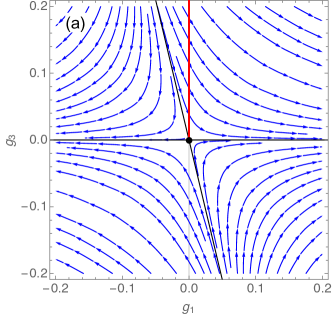
(a)

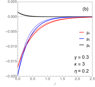
(b)

Figure 1: RG flow in the vicinity of the Gaussian fixed point. Panel (a): RG flow in the intersection of the subspace $\{g_{1},g_{3}\}$ and the hyperplane $g_{4}=g_{5}=g_{6}=0$. Black dot marks the Gaussian fixed point. Thin black lines indicate the eigenvectors of the linearized flow and the red line shows possible initial conditions $g_{1}(0)=0$, $g_{3}(0)>0$ [see Eq. (47)]. Panel (b): RG flow of $g_{4}$, $g_{5}$, and $g_{6}$ as given by Eq. (46) [solid lines] and Eq. (50) [dotted lines] for typical values of $\kappa$, $\gamma$, and $\eta$. The ratio $\Lambda/mv_{F}$ is $1$.

Let us now analyze the system of RG equations in the vicinity of the Gaussian fixed point fixed_points . Eqs. (46) can be written in the matrix form as $\partial_{l}\boldsymbol{g}=\boldsymbol{\beta}(\boldsymbol{g})$. The Jacobian matrix for the system linearized near the origin is

$$\boldsymbol{J}=\frac{\partial\left(\beta_{1},\beta_{3},\ldots,\beta_{6}\right)}{\partial\left(g_{1},g_{3},\ldots,g_{6}\right)}\Bigl{|}_{0}=\begin{pmatrix}\,1&\frac{3}{2\pi}&&&\\ &-1&&\frac{5}{\pi}&\\ &&-2&&\frac{15}{2\pi}\\ &&&-3&\\ &&&&-4\,\end{pmatrix}.$$ (49)

Then, the solution of the linearized system is $\boldsymbol{g}(l)=e^{l\boldsymbol{J}}\boldsymbol{g}_{0}$. In components it reads

$$g_{1}(l) =\frac{3}{2\pi}\,g_{3}(0)\,\sinh{l}+\frac{15}{4\pi^{2}}\,g_{5}(0)\,e^{-l}\sinh^{2}{l},$$ (50)

$$g_{3}(l) =g_{3}(0)\,e^{-l}+\frac{5}{\pi}\,g_{5}(0)\,e^{-2l}\sinh{l},$$

$$g_{4}(l) =g_{4}(0)\,e^{-2l}+\frac{15}{2\pi}\,g_{6}(0)\,e^{-3l}\sinh{l},$$

$$g_{5}(l) =g_{5}(0)\,e^{-3l},$$

$$g_{6}(l) =g_{6}(0)\,e^{-4l}.$$

Therefore, the system experiences a runaway flow, as seen in Fig. 2. This situation is typical for the first order phase transition Fisher1982 ; Binder1987 .

V Phase transition criterion

In order to obtain the phase transition criterion, let us consider the renormalized action that reads:

$$S=\int dxd\tau \left\{\frac{A}{2}\dot{\Phi}_{\sigma}^{2}+\frac{u_{2}}{2}\Phi_{\sigma}^{\prime}{}^{2}+u_{4}\Phi_{\sigma}^{\prime}{}^{4}+u_{6}\Phi_{\sigma}^{\prime}{}^{6}\right.$$ (51)

$$+u_{1}\Phi_{\sigma}^{\prime}+u_{3}\Phi_{\sigma}^{\prime}{}^{3}+u_{5}\Phi_{\sigma}^{\prime}{}^{5}\Bigr{\}},$$

where the coefficients $u_{j}=u_{j}(l)$ are the solutions to RG equations (43), and are related to the dimensionless couplings $g_{j}$ via Eqs. (41) and (45).

Before we proceed, let us make an important remark. One should keep in mind that in the context of ultracold atomic gases, magnetization is nothing else than the difference between the number of atoms in the (pseudo)spin-$\uparrow$ and -$\downarrow$ states. This means that the population of each spin species is conserved. Restricting ourselves to the case with no population imbalance, the total magnetization is zero in all phases:

$$\int dx\,\Phi_{\sigma}^{\prime}(x)=0.$$ (52)

Therefore, the linear term in action (51) should be discarded. Note that although condition (52) prohibits phases with nonzero total magnetization, it still allows the existence of spin configurations, where the magnetization is different from zero locally. In other words, one can have a system of domains.

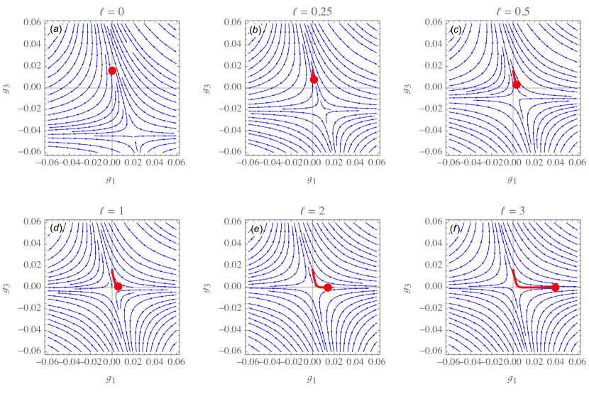
Figure 2: A step-by-step RG flow in the intersection of the $\{g_{1},g_{3}\}$ subspace and the hyperplane defined by the values of $g_{4}(l)$, $g_{5}(l)$, and $g_{6}(l)$ at a given $l$. The red dot represents the corresponding state of the system. Panel (a) shows the initial state of the system, $l=0$ and all couplings $g_{i}$ having their initial values $g_{i,0}$, as given by Eq. (47). Here we take typical values $\kappa=3$, $\gamma=0.3$, $\eta\approx 0.2$, and put $\Lambda/mv_{F}=1$ [the same as in Fig. 1 (b)]. In the consequent panels (b)–(f) the RG time $l$ increases, and the hyperplane $\{g_{4}(l),g_{5}(l),g_{6}(l)\}$ evolves according to the RG equations (46). This explains the variation of the flow lines from one panel to another [most noticeble in (a) – (d)]. The red line shows the path travelled by the system as it flows from the initial state at $l=0$ to the current state. After $l\gtrsim 1$, the couplings $g_{4}$, $g_{5}$, and $g_{6}$ are essentially zero, and in panels (d)–(f) the flow lines in the $\{g_{1},g_{3}\}$ plane remain practically the same.

At sufficiently large RG times $l$, in order to find the phase transition, one may simply minimize the renormalized Hamiltonian density Kozii2017 . The latter follows from Eq. (51) and reads

$${\cal H}=\frac{u_{2}}{2}\Phi_{\sigma}^{\prime}{}^{2}+u_{3}\Phi_{\sigma}^{\prime}{}^{3}-|u_{4}|\Phi_{\sigma}^{\prime}{}^{4}+u_{5}\Phi_{\sigma}^{\prime}{}^{5}+u_{6}\Phi_{\sigma}^{\prime}{}^{6},$$ (53)

where we omitted the kinetic term $\Pi_{\sigma}/2A$. At $l=0$ coefficients $u_{3}$ and $u_{5}$ are $\sim(\eta\kappa)^{5/2}$, and they are negligibly small for $\eta\kappa\ll 1$ [see Eq. (36)]. At larger $l$ these coefficients become even smaller. For this reason, we can neglect cubic and quintic terms in the Hamiltonian (53). Thus, up to small corrections, the phase transition criterion is

$$\frac{u_{2}(l)u_{6}(l)}{u_{4}^{2}(l)}\approx\frac{1}{2}.$$ (54)

In the region, where $u_{2}u_{6}/u_{4}^{2}<1/2$, the system is in the phase with zero magnetization $\langle\Phi^{\prime}\rangle$, whereas for $u_{2}u_{6}/u_{4}^{2}>1/2$ the ground state has $\langle\Phi^{\prime}\rangle\neq 0$.

Using Eq. (41) we express $u_{4}$ and $u_{6}$ in terms of the dimensionless couplings $g_{4}$ and $g_{6}$, and equation (54) becomes $g_{6}(l)/g_{4}^{2}(l)=\pi/2$. Here $g_{4}(l)$ and $g_{6}(l)$ are the solutions of RG equations (46). In the viscinity of the Gaussian fixed point the RG flow is such that it is well described by the linearized RG equations with the solutions (50), as can be seen from Fig. 1(b). Thus, the phase transition criterion (54) can be written as

$$\frac{g_{6}(0)}{g_{4}^{2}(0)}\;\frac{1}{1-\delta(l)}=\frac{\pi}{2},$$ (55)

where the bare couplings $g_{4}(0)$ and $g_{6}(0)$ are given by Eq. (47), and we introduced the quantity

$$\delta(l)=\frac{\pi\Lambda^{2}}{4(mv_{F})^{2}}\frac{(2-7y)\,e^{-l}\sinh l}{\left(2-y\right)^{1/2}\left(2+y/K_{\sigma}^{2}\right)^{1/2}(1-2y)}.$$ (56)

From Eqs. (55) and (56) we see that the distance to the phase transition is controlled by the parameter $y$, given by Eq. (37).

At $l=0$ the correction $\delta(l)$ is zero and Eq. (55) reduces to

$$\frac{(1-y/2)(1-7y/2)}{(1-2y)^{2}}=\frac{1}{16},$$ (57)

where we used Eq. (47) for $g_{4}(0)$ and $g_{6}(0)$. Eq. (57) is essentially the mean field phase transition criterion, since it involves only the bare couplings. The roots of Eq. (57) are $y=(5\pm\sqrt{15})/4$. Taking the minus sign we have $y_{*}\approx 0.282$. Thus, at the mean field level there is a first order phase transition at $y_{*}=0.282$, which can be the case at fairly weak coupling.

At finite values of $l$ and for $y$ sufficiently close to $y_{*}$, one has $\delta(l)\ll 1$. This is because $\Lambda/mv_{F}\sim 1$ and the $l$-dependent factor in Eq. (56) is bounded by $1/2$. We then look for the solution of Eq. (55) in the form $y=y_{*}+\delta y$ and obtain

$$\delta y\sim 10^{-4}(\Lambda/mv_{F})^{2}e^{-l}\sinh l\sim 10^{-4}.$$ (58)

We see that the correction $\delta y$ to the mean field critical value $y_{*}\approx 0.282$ is negligibly small. One may easily check that in this case the correction $\delta(l)$ is also negligible, being of the order of $10^{-2}$.

Thus, the phase transition criterion is given by Eq. (57), and the RG corrections can be neglected. The spontaneous magnetization in this case is

$${\cal M}\equiv\langle\Phi_{\sigma}^{\prime}\rangle=\pm\sqrt{u_{2}/|u_{4}|}.$$ (59)

Importantly, there are two minima, and hence it is possible to have an instanton-like field configuration that tunnels from one minimum to another, creating a sequence of domains (see, e.g., Rajaraman ).

As illustrated in Fig. 3, for $y<y_{*}\approx 0.282$ the system is in the phase with ${\cal M}=0$, whereas for $y>y_{*}$ the phase with a nonzero ${\cal M}$ has a lower energy.

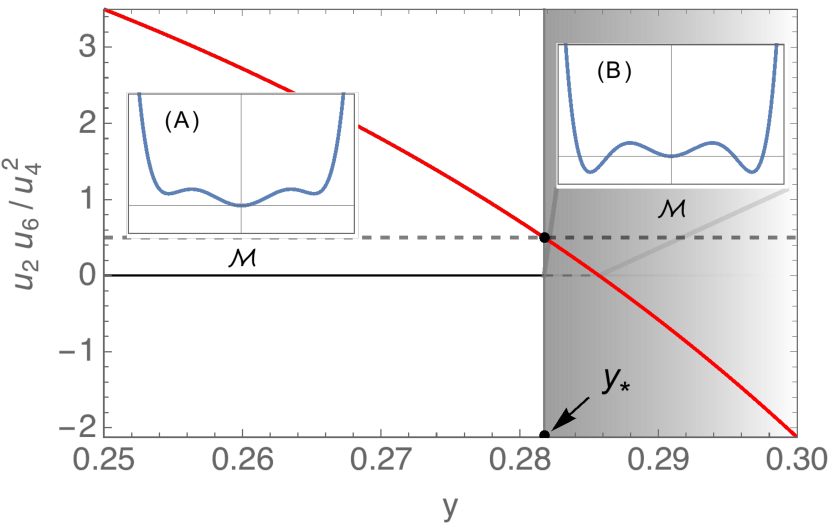
Figure 3: Phase diagram as follows from Eq. (57). The red line shows the ratio $g_{6}(0)/(\pi g_{4}(0)^{2})$ versus the dimensionless parameter $y$, given by Eq. (37). There is a critical value $y_{*}\approx 0.282$, where $g_{6}(0)/(\pi g_{4}(0)^{2})=1/2$ and the phase transition occurs. For $y<y_{*}$, the system is in the paramagnetic phase and the magnetization ${\cal M}$ is zero, as illustrated schematically on the inset (A). For $y>y_{*}$, the system enters the phase with the nonzero (local) magnetization ${\cal M}$, as shown on the inset (B).

VI Discussion and Conclusions

To summarize, in this paper we considered a zero temperature one-dimensional two-component Fermi gas with a weak/intermediate contact repulsive interaction in the even-wave channel and an additional attractive odd-wave interaction between particles in the spin-$\uparrow$ state. Using bosonization technique we derived an effective field theory for the spin degrees of freedom, described by the Lagrangian (35).

In the regime of weak/intermediate even-wave repulsion ($\gamma\lesssim 1$) and a near-resonant odd-wave attraction, we have found a first order phase transition to a state with a nonzero local magnetization. The distance to the phase transition is controlled by the dimensionless parameter $y$, given by Eq. (37). The phase transition occurs at the critical value $y_{*}\approx 0.282$. At smaller values the system is in the phase with zero magnetization. At larger values, in the region $y>y_{*}$, the system enters the phase with a nonzero local magnetization.

The phase with nonzero local magnetization deserves comments. In the context of ultracold atoms, the spin-$\uparrow$ and spin-$\downarrow$ states of a fermion are, actually, two distinct atomic hyperfine states. Magnetization in this language is then simply the difference between the populations of atoms in these states. In the absence of inelastic collisions this difference remains constant. Thus, when going through the phase transition, magnetization can change only locally, whereas the total magnetization remains zero. This is nothing else than the development of domains. In each domain there are more atoms in one hyperfine state than in the other. Therefore, locally, the magnetization is different from zero.

Appendix A The integral in Eq. (25)

In this Appendix we calculate the integral of the form

$$\tilde{\cal I}_{s,p}=\int_{0}^{+\infty}dx\,\int_{0}^{+\infty}dy\,e^{-\frac{x^{2}}{y}-\tilde{\nu}y}\frac{x^{s}y^{p-\frac{1}{2}}}{\left(x^{2}+y^{2}+a^{2}\right)^{K}}\qquad(K>0),$$ (60)

which is a slight generalization of the integral in Eq. (25). Using the well known identity

$$\frac{1}{\left(x^{2}+y^{2}+a^{2}\right)^{K}}=\frac{1}{\Gamma(K)}\int_{0}^{+\infty}dq\,q^{K-1}e^{-\left(x^{2}+y^{2}+a^{2}\right)\,q},$$ (61)

we write

$$\tilde{\cal I}_{s,p}=\frac{1}{\Gamma\left(K\right)}\int_{0}^{+\infty}dq\,e^{-a^{2}q}q^{K-1}\int_{0}^{+\infty}dy\,y^{p-\frac{1}{2}}\,e^{-\tilde{\nu}y-qy^{2}}\int_{0}^{+\infty}dx\,x^{s}\,e^{-\left(\frac{1}{y}+q\right)x^{2}}.$$ (62)

The integral over $dx$ gives

$$\frac{1}{2}\Gamma\left(\frac{s+1}{2}\right)\left(q+\frac{1}{y}\right)^{-(s+1)/2}$$ (63)

Then, taking the limit $a\to 0$ and making a change of variables $z=qy$ we obtain

$$\tilde{\cal I}_{s,p}=\frac{1}{2}\Gamma\left(\frac{s+1}{2}\right)\int_{0}^{+\infty}dy\,e^{-\tilde{\nu}y}\,y^{\frac{s}{2}+p-K}\frac{1}{\Gamma\left(K\right)}\int_{0}^{+\infty}dz\,e^{-yz}\,z^{K-1}\left(1+z\right)^{-(s+1)/2}.$$ (64)

In the integral over $dz$ one recognizes the integral representation of the Tricomi hypergeometric function. Its general form reads

$$U(\alpha,\beta,y)=\frac{1}{\Gamma(\alpha)}\int_{0}^{+\infty}dz\,e^{-yz}z^{\alpha-1}(1+z)^{\beta-\alpha-1},$$ (65)

which is valid for $\text{Re}\,y>0$ and $\text{Re}\,\alpha>0$. One has the following expression for $U(\alpha,\beta,y)$ in terms of the confluent hypergeometric function ${}_{1}F_{1}(\alpha,\beta,y)$:

$$U(\alpha,\beta,y)=\frac{\Gamma(1-\beta)}{\Gamma(\alpha-\beta+1)}\,_{1}F_{1}(\alpha,\beta,y)+\frac{\Gamma(\beta-1)}{\Gamma(\alpha)}\,y^{1-\beta}\,_{1}F_{1}(\alpha-\beta+1,2-\beta,y).$$ (66)

In our case we have $\alpha=K$ and $\beta=1+K-(s+1)/2$, which yields

$$\frac{1}{\Gamma\left(K\right)}\int_{0}^{+\infty}dz\,e^{-yz}\,z^{K-1}\left(1+z\right)^{-\frac{s+1}{2}}=U(K,1+K-\frac{s+1}{2},y)$$ (67)

$$=\frac{\Gamma\left(\frac{s+1}{2}-K\right)}{\Gamma\left(\frac{s+1}{2}\right)}\,_{1}F_{1}\left(K,1+K-\frac{s+1}{2},y\right)+\frac{\Gamma\left(K-\frac{s+1}{2}\right)}{\Gamma\left(K\right)}\,y^{\frac{s+1}{2}-K}\,_{1}F_{1}\left(\frac{s+1}{2},1+\frac{s+1}{2}-K,y\right)$$

Then, $\tilde{\cal I}_{s,p}$ becomes

$$\tilde{\cal I}_{s,p}=\frac{1}{2}\Gamma\left(\frac{s+1}{2}-K\right)J_{s,p}^{(1)}+\frac{\Gamma\left(\frac{s+1}{2}\right)\Gamma\left(K-\frac{s+1}{2}\right)}{2\Gamma\left(K\right)}J_{s,p}^{(2)},$$ (68)

where we defined

$$J_{s,p}^{(1)} =\int_{0}^{+\infty}dy\,e^{-\tilde{\nu}y}y^{\frac{s}{2}+p-K}\,_{1}F_{1}\left(K,\,1+K-\frac{s+1}{2},\,y\right),$$ (69)

$$J_{s,p}^{(2)} =\int_{0}^{+\infty}dy\,e^{-\tilde{\nu}y}y^{s+p+\frac{1}{2}-2K}\,_{1}F_{1}\left(\frac{s+1}{2},\,1-K+\frac{s+1}{2},\,y\right).$$

The above integrals can be calculated in terms of the ordinary hypergeometric function ${}_{2}F_{1}$ using LLvol3

$$\int_{0}^{+\infty}dy\,e^{-\lambda y}y^{\nu}\,_{1}F_{1}(\alpha,\beta,ky)=\Gamma(\nu+1)\lambda^{-\nu-1}\,_{2}F_{1}(\alpha,\nu+1,\beta,k/\lambda),$$ (70)

provided that $\text{Re}\,\nu>-1$ and $\text{Re}\,\lambda>|\text{Re}\,k|$. In the case $0<K\leq 1$ both these conditions are satisfied for $J_{s,p}^{(1)}$ and $J_{s,p}^{(2)}$ with any relevant combination of non-negative integers $s$ and $p$. Therefore, we finally obtain

$$J_{s,p}^{(1)} =\Gamma\left(\frac{s}{2}+p+1-K\right)\tilde{\nu}^{-\left(p+\frac{s}{2}-K+1\right)}\,_{2}F_{1}\left(K,\,\frac{s}{2}+p-K+1,1+K-\frac{s+1}{2},\frac{1}{\tilde{\nu}}\right),$$ (71)

$$J_{s,p}^{(2)} =\Gamma\left(s+p+\frac{3}{2}-2K\right)\tilde{\nu}^{-\left(p+s+\frac{3}{2}-2K\right)}\,_{2}F_{1}\left(\frac{s+1}{2},\,s+p+\frac{3}{2}-2K,1-K+\frac{s+1}{2},\frac{1}{\tilde{\nu}}\right).$$

Putting $K=1$ and $\tilde{\nu}=1/(\eta\kappa)$, we get

$$\tilde{\cal I}_{s,p} =\frac{1}{2}\Gamma\left(\frac{s+1}{2}-1\right)(\eta\kappa)^{p+\frac{s}{2}}\Gamma\left(p+\frac{s}{2}\right)\,_{2}F_{1}\left(1,p+\frac{s}{2};\frac{1}{2}(-s-1)+2;\eta\kappa\right)$$ (72)

$$+\frac{1}{2}\Gamma\left(\frac{1-s}{2}\right)\Gamma\left(\frac{s+1}{2}\right)\Gamma\left(p+\frac{s-1}{2}\right)(\eta\kappa)^{p+s-\frac{1}{2}}(1-\eta\kappa)^{-p-\frac{s}{2}+\frac{1}{2}}.$$

For $\eta\kappa\ll 1$ it behaves as

$$\tilde{\cal I}_{s,p}\approx\begin{cases}\frac{1}{2}\Gamma\left(\frac{s}{2}+p\right)\Gamma\left(\frac{s-1}{2}\right)(\eta\kappa)^{\frac{s}{2}+p},\quad s\neq 0;\\ \frac{\pi}{2}\Gamma\left(p-\frac{1}{2}\right)(\eta\kappa)^{p-\frac{1}{2}},\;\,\quad\quad\qquad s=0,\end{cases}$$ (73)

which leads to Eqs. (27) and (28) in the main text.

Appendix B Bosonized odd-wave interaction

In this Appendix we present the terms that we keep after expanding the $\Theta_{\rho,\sigma}$ fields and the normal-ordered exponent in Eq. (30). In the charge sector these are the terms up to the second order in the fields:

$$\delta{\cal L}_{\text{odd}}^{(\rho)}=-i\sqrt{2\pi}k_{F}\alpha_{0,1}\dot{\Theta}_{\rho}+\pi v_{F}^{-1}\alpha_{0,2}\dot{\Theta}_{\rho}^{2}+\pi v_{F}\alpha_{2,0}\Theta_{\rho}^{\prime}{}^{2}.$$ (74)

In the spin sector – up to the sixth order:

$$\delta{\cal L}_{\text{odd}}^{(\sigma)}=-i\sqrt{2\pi}k_{F}\alpha_{0,1}\dot{\Theta}_{\sigma}+\pi v_{F}^{-1}\alpha_{0,2}\dot{\Theta}_{\sigma}^{2}+\pi v_{F}\alpha_{2,0}\Theta_{\sigma}^{\prime}{}^{2}+\frac{\sqrt{2}\pi^{3/2}}{3mv_{F}^{3}}\alpha_{0,3}\,i\,\dot{\Theta}_{\sigma}^{3}-\frac{\pi}{4m^{2}v_{F}^{3}}\alpha_{2,2}\dot{\Theta}_{\sigma}^{\prime}{}^{2}$$ (75)

$$-\frac{\pi^{2}}{6m^{2}v_{F}^{5}}\alpha_{0,4}\dot{\Theta}_{\sigma}^{4}-\frac{\pi^{2}}{6m^{2}v_{F}}\alpha_{4,0}\Theta_{\sigma}^{\prime}{}^{4}-\frac{\pi^{5/2}}{15\sqrt{2}m^{3}v_{F}^{7}}\alpha_{0,5}\,i\,\dot{\Theta}_{\sigma}^{5}+\frac{\pi^{3}}{90m^{4}v_{F}^{9}}\alpha_{0,6}\dot{\Theta}_{\sigma}^{6}+\frac{\pi^{3}}{90m^{4}v_{F}^{3}}\alpha_{6,0}\Theta_{\sigma}^{\prime}{}^{6}.$$

Finally, we also keep the following terms that couple spin and charge:

$$\delta{\cal L}_{\text{odd}}^{(\rho\sigma)}=2\pi v_{F}\alpha_{2,0}\Theta^{\prime}_{\rho}\Theta^{\prime}_{\sigma}+\frac{2\pi}{v_{F}}\alpha_{0,2}\dot{\Theta}_{\rho}\dot{\Theta}_{\sigma}+\frac{\sqrt{2}\pi^{3/2}}{mv_{F}^{3}}\alpha_{0,3}i\dot{\Theta}_{\rho}\dot{\Theta}_{\sigma}^{2}+\frac{\sqrt{2}\pi^{3/2}}{mv_{F}}\alpha_{2,1}i\dot{\Theta}_{\rho}\Theta_{\sigma}^{\prime}{}^{2}.$$ (76)

Appendix C Effective Lagrangian for the spin fields

In this Appendix we integrate out the charge fields and obtain an effective Lagrangian for the spin degrees of freedom, given by Eq. (35) in the main text.

C.1 Total bosonized Lagrangian

Combining Eqs. (74), (75), and (76) with Eq. (19), we arrive to the total Lagrangian ${\cal L}={\cal L}_{\sigma}+{\cal L}_{\rho}^{(0)}+{\cal L}_{\rho\sigma}$ given by Eqs. (31) – (33) in the main text. The coefficients in the Lagrangian are given by

$$\varepsilon_{\rho}=\varepsilon_{\sigma}=\sqrt{2\pi}k_{F}\alpha_{0,1}\approx(\sqrt{2}/\pi)k_{F}\sqrt{\eta/\kappa}$$ (77)

$$\quad A_{2}^{\rho,\sigma}=\frac{K_{\rho,\sigma}}{u_{\rho,\sigma}}+\frac{2\pi\alpha_{0,2}}{v_{F}},\quad A_{3}^{\sigma}=\frac{\sqrt{2}\pi^{3/2}\alpha_{0,3}}{3mv_{F}^{3}},\quad A_{4}^{\sigma}=\frac{\Gamma^{2}}{8}\frac{K_{\rho}}{u_{\rho}}\frac{K_{\sigma}^{4}}{u_{\sigma}^{4}}+\frac{\pi^{2}\alpha_{0,4}}{6m^{2}v_{F}^{5}},\quad A_{5}^{\sigma}=\frac{\pi^{5/2}\alpha_{0,5}}{15\sqrt{2}m^{3}v_{F}^{7}},\quad A_{6}^{\sigma}=\frac{\pi^{3}\alpha_{0,6}}{90m^{4}v_{F}^{9}},\quad$$

$$B_{2}^{\rho,\sigma}=u_{\rho,\sigma}K_{\rho,\sigma}+2\pi v_{F}\alpha_{2,0},\quad B_{4}^{\sigma}=\frac{\Gamma^{2}}{8}\frac{K_{\rho}}{u_{\rho}}+\frac{\pi^{2}\alpha_{4,0}}{6m^{2}v_{F}},\quad B_{6}^{\sigma}=\frac{\pi^{3}\alpha_{6,0}}{90m^{4}v_{F}^{3}},$$

$$C=2\pi v_{F}\alpha_{2,0},\quad D=\frac{2\pi}{v_{F}}\alpha_{0,2},\quad E=\frac{\Gamma}{2}\frac{K_{\rho}}{u_{\rho}}+\frac{\sqrt{2}\pi^{3/2}\alpha_{2,1}}{mv_{F}},\quad F=\frac{\Gamma}{2}\frac{K_{\rho}}{u_{\rho}}\frac{K_{\sigma}^{2}}{u_{\sigma}^{2}}-\frac{\sqrt{2}\pi^{3/2}\alpha_{0,3}}{mv_{F}^{3}}.$$

After the shift $\Theta_{\rho}=\tilde{\Theta}_{\rho}+i\beta_{\rho}\tau$, given by Eq. (34), the Lagrangian becomes

$${\cal L}_{\sigma}=ia_{1}^{\sigma}\dot{\Theta}_{\sigma}+\frac{a_{2}^{\sigma}}{2}\dot{\Theta}_{\sigma}^{2}+\frac{b_{2}^{\sigma}}{2}\Theta_{\sigma}^{\prime 2}+a_{3}^{\sigma}\,i\,\dot{\Theta}_{\sigma}^{3}-a_{4}^{\sigma}\dot{\Theta}_{\sigma}{}^{4}-b_{4}^{\sigma}\Theta_{\sigma}^{\prime}{}^{4}-a_{5}^{\sigma}\,i\,\dot{\Theta}_{\sigma}^{5}+a_{6}^{\sigma}\dot{\Theta}_{\sigma}^{6}+b_{6}^{\sigma}\Theta_{\sigma}^{\prime}{}^{6},$$ (78)

$${\cal L}^{(0)}_{\rho}=\frac{A_{2}^{\rho}}{2}\dot{\tilde{\Theta}}_{\rho}^{2}+\frac{B_{2}^{\rho}}{2}\tilde{\Theta}_{\rho}^{\prime 2},$$ (79)

$${\cal L}_{\rho\sigma}=C\tilde{\Theta}_{\rho}^{\prime}\Theta_{\sigma}^{\prime}+D\dot{\tilde{\Theta}}_{\rho}\dot{\Theta}_{\sigma}+i\,\dot{\tilde{\Theta}}_{\rho}\Bigl{\{}E{\Theta}_{\sigma}^{\prime}{}^{2}-F\dot{{\Theta}}_{\sigma}^{2}\Bigr{\}},$$ (80)

where

$$a_{1}^{\sigma}=D\beta_{\rho}-\varepsilon_{\sigma}=-\frac{K_{\rho}}{u_{\rho}}\beta_{\rho},\quad a_{2}^{\sigma}=A_{2}^{\sigma}+2F\beta_{\rho},\qquad a_{3}^{\sigma}=A_{3}^{\sigma},\quad a_{4}^{\sigma}=A_{4}^{\sigma},\qquad a_{5}^{\sigma}=A_{5}^{\sigma},\qquad a_{6}^{\sigma}=A_{6}^{\sigma}$$ (81)

$$b_{2}^{\sigma}=B_{2}^{\sigma}-2E\beta_{\rho},\quad b_{4}^{\sigma}=B_{4}^{\sigma},\quad b_{6}^{\sigma}=B_{6}^{\sigma}.$$

Since primarily we are interested in the spin sector, we proceed with integrating out the charge fields.

C.2 Integration over the charge degrees of freedom

The partition function can be written as

$${\cal Z}=\int{\cal D}\Theta_{\sigma}\,e^{-\int dxd\tau{\cal L}_{\sigma}}\int{\cal D}\tilde{\Theta}_{\rho}\,e^{-\int dxd\tau{\cal L}_{\rho}^{(0)}-\int dxd\tau{\cal L}_{\rho\sigma}},$$ (82)

where the Lagrangian is given by Eqs. (78) – (80). The integral over ${\cal D}\tilde{\Theta}_{\rho}$ is Gaussian and, formally, can be calculated exactly. We first write the action corresponding to ${\cal L}_{\rho}^{0}$ as

$$S_{\rho}^{(0)}=\frac{1}{2}\int dxd\tau\,\tilde{\Theta}_{\rho}(x,\tau)\left\{-B_{2}^{\rho}\left(\partial_{x}^{2}+\frac{A_{2}^{\rho}}{B_{2}^{\rho}}\partial^{2}_{\tau}\right)\right\}\tilde{\Theta}_{\rho}(x,\tau)=\frac{1}{2}\int d1d2\tilde{\Theta}_{\rho}(1)G^{-1}_{\rho}(1-2)\tilde{\Theta}_{\rho}(2),$$ (83)

where $d1=dx_{1}d\tau_{1}$, $d2=dx_{2}d\tau_{2}$, and the Green’s function is

$$G_{\rho}(x,\tau)=-\frac{1}{4\pi\sqrt{A_{2}^{\rho}B_{2}^{\rho}}}\ln\frac{x^{2}+(B_{2}^{\rho}/A_{2}^{\rho})\tau^{2}+a^{2}}{a^{2}}.$$ (84)

The action corresponding to ${\cal L}_{\rho\sigma}$, i.e. terms that couple spin and charge, we write as

$$S_{\rho\sigma}=\int dxd\tau\tilde{\Theta}_{\rho}\left[-C\Theta_{\sigma}^{\prime\prime}-D\ddot{\Theta}_{\sigma}-i\,\partial_{\tau}\left(E\Theta_{\sigma}^{\prime 2}-F\dot{\Theta}_{\sigma}^{2}\right)\right]\equiv\int dxd\tau\tilde{\Theta}_{\rho}{\cal J}_{\sigma}.$$ (85)

Then, the integral over ${\cal D}\tilde{\Theta}_{\rho}$ takes the standard form and yields

$$\int{\cal D}\tilde{\Theta}_{\rho}\exp\left\{-\frac{1}{2}\int d1d2\tilde{\Theta}_{\rho}(1)G^{-1}_{\rho}(1-2)\tilde{\Theta}_{\rho}(2)+\int d1\tilde{\Theta}_{\rho}(1){\cal J}_{\sigma}(1)\right\}\propto\exp\left\{\frac{1}{2}\int d1d2{\cal J}_{\sigma}(1)G_{\rho}(1-2){\cal J}_{\sigma}(2)\right\}.$$ (86)

Thus, integration over the charge degrees of freedom provides the following correction to $S_{\sigma}$:

$$\delta S=-\frac{1}{2}\int d1d2{\cal J}_{\sigma}(1)G_{\rho}(1-2){\cal J}_{\sigma}(2)\to\sum_{j=1}^{4}\delta S_{j},$$ (87)

where we kept only the most relevant terms:

$$\delta S_{1} =-\frac{C^{2}}{2}\int d1d2\,\partial_{x_{1}}^{2}\Theta_{\sigma}(1)G_{\rho}(1-2)\,\partial_{x_{2}}^{2}\Theta_{\sigma}(2)=+\frac{C^{2}}{2}\int d1d2\,\partial_{x_{1}}\Theta_{\sigma}(1)G^{\prime\prime}_{\rho}(1-2)\,\partial_{x_{2}}\Theta_{\sigma}(2),$$ (88)

$$\delta S_{2} =-\frac{D^{2}}{2}\int d1d2\,\partial_{\tau_{1}}^{2}\Theta_{\sigma}(1)G_{\rho}(1-2)\,\partial_{\tau_{2}}^{2}\Theta_{\sigma}(2)=+\frac{D^{2}}{2}\int d1d2\,\partial_{\tau_{1}}\Theta_{\sigma}(1)\ddot{G}_{\rho}(1-2)\,\partial_{\tau_{2}}\Theta_{\sigma}(2),$$

$$\delta S_{3} =+\frac{E^{2}}{2}\int d1d2\,\partial_{\tau_{1}}\left(\partial_{x_{1}}\Theta_{\sigma}(1)\right)^{2}G_{\rho}(1-2)\,\partial_{\tau_{2}}\left(\partial_{x_{2}}\Theta_{\sigma}(2)\right)^{2}$$

$$=-\frac{E^{2}}{2}\int d1d2\,\left(\partial_{x_{1}}\Theta_{\sigma}(1)\right)^{2}\ddot{G}_{\rho}(1-2)\,\left(\partial_{x_{2}}\Theta_{\sigma}(2)\right)^{2},$$

$$\delta S_{4} =+\frac{F^{2}}{2}\int d1d2\,\partial_{\tau_{1}}\left(\partial_{\tau_{1}}\Theta_{\sigma}(1)\right)^{2}G_{\rho}(1-2)\,\partial_{\tau_{2}}\left(\partial_{\tau_{2}}\Theta_{\sigma}(2)\right)^{2}$$

$$=-\frac{F^{2}}{2}\int d1d2\,\left(\partial_{\tau_{1}}\Theta_{\sigma}(1)\right)^{2}\ddot{G}_{\rho}(1-2)\,\left(\partial_{\tau_{2}}\Theta_{\sigma}(2)\right)^{2}.$$

Using the results of subsection C.3, for the above terms we obtain:

$$\delta S_{1} =-\frac{C^{2}}{4B_{2}^{\rho}}\int d\tau dx\,\Theta_{\sigma}^{\prime 2},\qquad\qquad\qquad\delta S_{2}=-\frac{D^{2}}{4A_{2}^{\rho}}\int d\tau dx\,\dot{\Theta}_{\sigma}^{2},$$ (89)

$$\delta S_{3} =+\frac{E^{2}}{4A_{2}^{\rho}}\int d\tau dx\,\Theta_{\sigma}^{\prime 4},\qquad\qquad\delta S_{4}=+\frac{F^{2}}{4A_{2}^{\rho}}\int d\tau dx\,\dot{\Theta}_{\sigma}^{4}.$$

Therefore, combining the above corrections with Eq. (78), the dual filed representation of the effective Lagrangian for the spin degrees of freedom becomes:

$$\tilde{\cal L}_{\sigma}=ia_{1}\dot{\Theta}_{\sigma}+\frac{a_{2}}{2}\dot{\Theta}_{\sigma}^{2}+\frac{b_{2}}{2}\Theta_{\sigma}^{\prime 2}+i\frac{a_{3}}{3}\dot{\Theta}_{\sigma}^{3}-\frac{a_{4}}{4}\dot{\Theta}_{\sigma}^{4}-\frac{b_{4}}{4}\Theta_{\sigma}^{\prime 4}-i\frac{a_{5}}{5}\dot{\Theta}_{\sigma}^{5}+\frac{a_{6}}{6}\dot{\Theta}_{\sigma}^{6}+\frac{b_{6}}{6}\Theta_{\sigma}^{\prime}{}^{6},$$ (90)

where we defined

$$a_{1}=a_{1}^{\sigma},\quad a_{2}=a_{2}^{\sigma}-\frac{D^{2}}{2A_{2}^{\rho}},\quad b_{2}=b_{2}^{\sigma}-\frac{C^{2}}{2B_{2}^{\rho}},\quad a_{3}=3a_{3}^{\sigma},\quad a_{4}=4a_{4}^{\sigma}-\frac{F^{2}}{A_{2}^{\rho}},\quad b_{4}=4b_{4}^{\sigma}-\frac{E^{2}}{A_{2}^{\rho}},\quad a_{5}=5a_{5}^{\sigma},$$ (91)

$$a_{6}=6a_{6}^{\sigma},\quad b_{6}=6b_{6}^{\sigma}.$$

Using Eqs. (77) and (81) one can see that all quadratic terms have strictly positive coefficients, whereas all quartic terms – strictly negative coefficients.

C.3 Derivation of Eq. (89)

Here we show that

$$\int d\tau_{1}d\tau_{2}dx_{1}dx_{2}f(x_{1},\tau_{2})G^{\prime\prime}_{\rho}(x_{1}-x_{2},\tau_{1}-\tau_{2})f(x_{2},\tau_{2})\approx-\frac{1}{2B_{2}^{\rho}}\int d\tau dxf^{2}(x,\tau),$$ (92)

$$\int d\tau_{1}d\tau_{2}dx_{1}dx_{2}f(x_{1},\tau_{2})\ddot{G}_{\rho}(x_{1}-x_{2},\tau_{1}-\tau_{2})f(x_{2},\tau_{2})\approx-\frac{1}{2A_{2}^{\rho}}\int d\tau dxf^{2}(x,\tau),$$

given that the Green’s function satisfies

$$\Bigl{(}\partial_{x}^{2}+(A_{2}^{\rho}/B_{2}^{\rho})\partial_{\tau}^{2}\Bigr{)}\,G_{\rho}(x,\tau)=-\frac{1}{B_{2}^{\rho}}\delta^{2}(x,\tau).$$ (93)

Going to the relative and the center of mass coordinates, we write the first integral as

$$\int dTdXdtdx\,\partial_{x}^{2}\,G_{\rho}(x,t)\,f(X+\frac{x}{2},T+\frac{t}{2})f(X-\frac{x}{2},T-\frac{t}{2})\approx\int dtdxG^{\prime\prime}_{\rho}(x,t)\int dTdXf^{2}(X,T).$$ (94)

Rescaling $y=\sqrt{B_{2}^{\rho}/A_{2}^{\rho}}\tau$ brings the equation for $G_{\rho}(x,y)$ to

$$\Delta_{x,y}G_{\rho}(x,y)=-\frac{1}{\sqrt{A_{2}^{\rho}B_{2}^{\rho}}}\delta^{2}(x,y).$$ (95)

Since $G_{\rho}$ only depends on $r=\sqrt{x^{2}+y^{2}}$, in polar coordinates we have

$$\left(\partial_{r}^{2}+\frac{1}{r}\partial_{r}\right)G_{\rho}(r)=\Delta_{r}G_{\rho}(r)=-\frac{1}{\sqrt{A_{2}^{\rho}B_{2}^{\rho}}}\frac{\delta(r)}{2\pi r}.$$ (96)

Then, taking into account that

$$\partial_{x}^{2}G_{\rho}(x,y)=\frac{1}{2}\Delta_{r}G_{\rho}(r)+\frac{\cos 2\phi}{2}\left(\partial_{r}^{2}-\frac{1}{r}\partial_{r}\right)$$ (97)

and the second term vanishes after the integration over the polar angle $\phi$, we write the integral $\int dxdtG_{\rho}^{\prime\prime}(x,t)$ in polar coordinates and get

$$\int dtdxG^{\prime\prime}_{\rho}(x,t)=2\pi\sqrt{\frac{A_{2}^{\rho}}{B_{2}^{\rho}}}\int_{0}^{+\infty}rdr\frac{1}{2}\Delta_{r}G_{\rho}(r)=-\frac{1}{2B_{2}^{\rho}}.$$ (98)

which yields the first result stated in the beginning of the Appendix. The proof for the second one is identical.

C.4 Effective spin Lagrangian in the $\Phi_{\sigma}$-representation

Let us now rewrite the Lagrangian $\tilde{\cal L}_{\sigma}$ from Eq. (90) in the $\Phi$-representation. We begin by writing the corresponding Hamiltonian in the $\Theta$-representation (we omit the index $\sigma$, since we do not have the charge fields anymore):

$${\cal H}(\Pi_{\Theta},\Theta^{\prime})=\Bigl{(}\tilde{\cal L}+i\dot{\Theta}\Pi_{\Theta}\Bigr{)}\Bigr{|}_{\dot{\Theta}=\dot{\Theta}\left(\Pi_{\Theta}\right)}\,\,,$$ (99)

where the expression for $\dot{\Theta}$ in terms of $\Pi_{\Theta}$ follows from

$$i\Pi_{\Theta}=-\frac{\partial\tilde{\cal L}_{\sigma}}{\partial\dot{\Theta}}=-ia_{1}-a_{2}\dot{\Theta}-ia_{3}\dot{\Theta}^{2}+a_{4}\dot{\Theta}^{3}+ia_{5}\dot{\Theta}^{4}-a_{6}\dot{\Theta}^{5}.$$ (100)

Since $\Pi_{\Theta}=-\Phi^{\prime}$, one can also rewrite the above relation as

$$\dot{\Theta}=\frac{1}{a_{2}}\Bigl{\{}\,i\,\left(\Phi^{\prime}-a_{1}\right)-ia_{3}\dot{\Theta}^{2}+a_{4}\dot{\Theta}^{3}+ia_{5}\dot{\Theta}^{4}-a_{6}\dot{\Theta}^{5}\Bigr{\}}.$$ (101)

Then, using Eqs. (99), (100), and taking into account that $\Theta^{\prime}=-\Pi_{\Phi}$, the $\Phi$-representation for the Hamiltonian can be formally written as

$${\cal H}=\frac{b_{2}}{2}\Pi_{\Phi}^{2}-\frac{b_{4}}{4}\Pi_{\Phi}^{4}+\frac{b_{6}}{6}\Pi_{\Phi}^{6}+\Bigl{(}-\frac{a_{2}}{2}\dot{\Theta}^{2}-i\frac{2a_{3}}{3}\dot{\Theta}^{3}+\frac{3a_{4}}{4}\dot{\Theta}^{4}+i\frac{4a_{5}}{5}\dot{\Theta}^{5}-\frac{5a_{6}}{6}\dot{\Theta}^{6}\Bigr{)}\Bigr{|}_{\dot{\Theta}=\dot{\Theta}\left(\Phi^{\prime}\right)}\,\,,$$ (102)

with $\dot{\Theta}$ being expressed via $\Phi^{\prime}$ using Eq. (101). Now, solving Eq. (101) for $\dot{\Theta}$ in terms of $\Phi^{\prime}$ by iterations, we get

$$\dot{\Theta} =\frac{i}{a_{2}}\Phi^{\prime}+i\frac{a_{3}}{a_{2}^{3}}\Phi^{\prime}{}^{2}-i\frac{a_{2}a_{4}-2a_{3}^{2}}{a_{2}^{5}}\Phi^{\prime}{}^{3}+i\frac{5a_{3}^{3}-5a_{2}a_{4}a_{3}+a_{2}^{2}a_{5}}{a_{2}^{7}}\Phi^{\prime}{}^{4}$$ (103)

$$+i\,\frac{14a_{3}^{4}-21a_{2}a_{4}a_{3}^{2}+6a_{2}^{2}a_{5}a_{3}+a_{2}^{2}\left(3a_{4}^{2}-a_{2}a_{6}\right)}{a_{2}^{9}}\,\Phi^{\prime}{}^{5}.$$

The potential part of Hamiltonian (102) becomes

$$\frac{1}{2a_{2}}\Phi^{\prime}{}^{2}+\frac{a_{3}}{3a_{2}^{3}}\Phi^{\prime}{}^{3}+\frac{2a_{3}^{2}-a_{2}a_{4}}{4a_{2}^{5}}\Phi^{\prime}{}^{4}+\frac{5a_{3}^{3}-5a_{2}a_{4}a_{3}+a_{2}^{2}a_{5}}{5a_{2}^{7}}{\Phi}^{\prime}{}^{5}+\frac{14a_{3}^{4}-21a_{2}a_{4}a_{3}^{2}+6a_{2}^{2}a_{5}a_{3}+3a_{2}^{2}a_{4}^{2}-a_{2}^{3}a_{6}}{6a_{2}^{9}}{\Phi}^{\prime}{}^{6}$$ (104)

The Lagrangian in the $\Phi$-representation is then

$$\tilde{\cal L}(\dot{\Phi},\Phi^{\prime})=\Bigl{(}{\cal H}\left(\Pi_{\Phi},\Phi^{\prime}\right)-i\dot{\Phi}\Pi_{\Phi}\Bigr{)}\Bigr{|}_{\Pi_{\Phi}=\Pi_{\Phi}(\dot{\Phi})}\,\,,$$ (105)

where $\Pi_{\phi}$ is relates to $\dot{\Phi}$ via

$$i\dot{\Phi}=\frac{\partial{\cal H}}{\partial\Pi_{\Phi}}=b_{2}\Pi_{\Phi}-b_{4}\Pi_{\Phi}^{3}+b_{6}\Pi_{\Phi}^{5}.$$ (106)

The latter can be written as

$$\Pi_{\Phi}=\frac{1}{b_{2}}\left(i\dot{\Phi}+b_{4}\Pi_{\Phi}^{3}-b_{6}\Pi_{\Phi}^{5}\right).$$ (107)

Solving by iterations, we get

$$\Pi_{\Phi}=\frac{i}{b_{2}}\dot{\Phi}\left(1-\frac{b_{4}}{b_{2}^{3}}\dot{{\Phi}}^{2}-\frac{b_{2}b_{6}-3b_{4}^{2}}{b_{2}^{6}}\dot{{\Phi}}^{4}\right).$$ (108)

The kinetic part of Hamiltonian (102) then gives

$$\frac{b_{2}}{2}\Pi_{\Phi}^{2}-\frac{b_{4}}{4}\Pi_{\Phi}^{4}+\frac{b_{6}}{6}\Pi_{\Phi}^{6}=\frac{\dot{{\Phi}}^{2}}{2b_{2}}-\frac{b_{4}}{4b_{2}^{4}}\dot{{\Phi}}^{4}+\frac{3b_{4}^{2}-b_{2}b_{6}}{6b_{2}^{7}}\dot{{\Phi}}^{6}.$$ (109)

Thus, using Eq. (105) we finally arrive at the Lagrangian given by (35) in the main text:

$$\tilde{\cal L}(\dot{\Phi},\Phi^{\prime}) =\frac{1}{2b_{2}}\dot{{\Phi}}^{2}+\frac{1}{2a_{2}}\Phi^{\prime}{}^{2}+\frac{a_{3}}{3a_{2}^{3}}\Phi^{\prime}{}^{3}+\frac{2a_{3}^{2}-a_{2}a_{4}}{4a_{2}^{5}}\Phi^{\prime}{}^{4}$$ (110)

$$+\frac{5a_{3}^{3}-5a_{2}a_{4}a_{3}+a_{2}^{2}a_{5}}{5a_{2}^{7}}{\Phi}^{\prime}{}^{5}+\frac{14a_{3}^{4}-21a_{2}a_{4}a_{3}^{2}+6a_{2}^{2}a_{5}a_{3}+3a_{2}^{2}a_{4}^{2}-a_{2}^{3}a_{6}}{6a_{2}^{9}}{\Phi}^{\prime}{}^{6}$$

$$\equiv\frac{A}{2}\dot{\Phi}^{2}+\frac{u_{2}}{2}\Phi^{\prime 2}+\sum_{n=3}^{6}u_{n}\Phi^{\prime}{}^{n}.$$

Appendix D Momentum-shell RG

In this Appendix we present a detailed derivation of the RG equations within the momentum-shell approach. We begin by considering the action in Eq. (39) of the main text:

$$S[\Phi]=S_{0}[\Phi]+S_{1}[\Phi]$$ (111)

$$=\int dxd\tau\left\{\frac{A}{2}\dot{\Phi}^{2}+\frac{u_{2}}{2}\Phi^{\prime 2}\right\}+\int dxd\tau\sum_{n=3}^{6}u_{n}\Phi^{\prime n}$$

and expand the field into the slow and fast components as $\Phi=\Phi_{<}+\Phi_{>}$. The slow component $\Phi_{<}$ has momentum modes in the interval $0<|k|<\Lambda/b$, whereas the fast component $\Phi_{>}$ — in the interval $\Lambda/b<|k|<\Lambda$, where $\Lambda$ is the UV momentum cutoff and $b=\exp{(\delta l)}$ is the scaling factor. In the Gaussian part of the action the slow and fast components decouple: $S_{0}[\Phi]=S_{0<}+S_{0>}$. For the interaction part we have $S_{1}[\Phi_{<}+\Phi_{>}]=S_{1<}+\tilde{S}[\Phi_{<},\Phi_{>}]$, where

$$\tilde{S}[\Phi_{<},\Phi_{>}]=\int dxd\tau\sum_{n=3}^{6}u_{n}\sum_{p=1}^{n}{n\choose p}\Phi^{\prime n-p}_{<}\Phi^{\prime p}_{>}.$$ (112)

Thus, the total action becomes $S[\Phi]=S_{<}+S_{0>}+\tilde{S}$. Then, expanding the partition function to second order in $\tilde{S}$, we obtain

$${\cal Z}=\int{\cal D}\Phi_{<}e^{-S_{<}-\langle\tilde{S}\rangle_{0>}+\frac{1}{2}\langle\tilde{S}^{2}\rangle_{0>}^{c}},$$ (113)

where $\langle\tilde{S}^{2}\rangle_{0>}^{c}=\langle\tilde{S}^{2}\rangle_{0>}-\langle\tilde{S}\rangle_{0>}^{2}$ and $\langle\ldots\rangle_{0>}$ is the average over the fast components $\Phi_{>}$ with the Gaussian action $S_{0>}$. In the above expression we omitted the constant contribution $\ln{\cal Z}_{0>}$.

D.1 First order correction

For the first order correction $\langle\tilde{S}\rangle_{0>}$ we need to calculate

$$\sum_{n=3}^{6}\sum_{p=1}^{n}u_{n}{n\choose p}\Phi^{\prime n-p}_{<}\langle\Phi^{\prime p}_{>}\rangle_{0>}.$$ (114)

We immediately see that for $n=3,4$ we only need terms with $p=2$, and for $n=5,6$ only terms with $p=2,4$. Other terms either vanish upon averaging or give constant contribution independent of $\Phi^{\prime}_{<}$. Let us first consider $p=2$ and calculate the corresponding Green’s function $G_{0>}\equiv\langle\Phi^{\prime 2}_{>}\rangle_{0>}$:

$$G_{0>}=\int_{-\infty}^{+\infty}\frac{d\omega}{2\pi}\int_{>}\frac{dk}{2\pi}\frac{k^{2}}{A\omega^{2}+u_{2}k^{2}}.$$ (115)

In the above expression we used a short-hand notation

$$\int_{>}\frac{dk}{2\pi}\equiv\int\displaylimits_{\Lambda/b<|k|<\Lambda}\frac{dk}{2\pi}.$$ (116)

Integrating over $d\omega$ and taking into account that $b\approx 1+\delta l$, we get

$$G_{0>}=\frac{1}{2\pi}\frac{\Lambda^{2}}{(Au_{2})^{1/2}}\delta l\equiv{\cal G}_{1}\delta l.$$ (117)

Consider now terms with $p=4$. Using Wick’s theorem one has $\langle\Phi^{\prime 4}_{>}\rangle_{0>}=3G_{0>}^{2}$, which is $\sim\delta l^{2}$. Such terms do not contribute to the RG equations, derived in the limit $\delta l\to 0$. Therefore, for the first order correction $\langle\tilde{S}\rangle_{0>}$ we only need terms with $p=2$:

$$\langle\tilde{S}\rangle_{0>}={\cal G}_{1}\delta l\int dxd\tau \bigl{\{}3u_{3}\Phi^{\prime}_{<}+6u_{4}\Phi^{\prime 2}_{<}+$$ (118)

$$+10u_{5}\Phi^{\prime 3}_{<}+15u_{6}\Phi^{\prime 4}_{<}\bigr{\}}.$$

Note that a new term $\sim\Phi^{\prime}_{<}$ has been generated. However, including it into the action does not lead to any new terms coming from $\langle\tilde{S}\rangle_{0>}$, as can be easily seen from Eq. (114). We will see later that this is also true for $\langle\tilde{S}^{2}\rangle_{0>}^{c}$.

D.2 Second order correction

We now turn to the calculation of the second order correction $\langle\tilde{S}^{2}\rangle_{0>}^{c}$. Explicitly, it reads

$$\langle\tilde{S}^{2}\rangle_{0>}^{c} =\int d1d2\sum_{n,m=3}^{6}\sum_{p=1}^{n}\sum_{q=1}^{m}{n\choose p}{m\choose q}u_{n}u_{m}$$ (119)

$$\times\Phi^{\prime n-p}_{<}(1)\Phi^{\prime m-q}_{<}(2)\,\langle\Phi^{\prime p}_{>}(1)\Phi^{\prime q}_{>}(2)\rangle_{0>}^{c},$$

where $d1d2\equiv dx_{1}d\tau_{1}dx_{2}d\tau_{2}$. Before doing any calculations, we note that applying Wick’s theorem to $\langle\Phi^{\prime p}_{>}(1)\Phi^{\prime q}_{>}(2)\rangle_{0>}^{c}$ will in general produce a number of terms of the form

$$\int d1d2\,\langle\Phi^{\prime}_{>}(1)\Phi^{\prime}_{>}(2)\rangle_{0>}^{N}\,\Phi^{\prime n-p}_{<}(1)\,\Phi^{\prime m-q}_{<}(2),$$ (120)

where the exponent $N$ depends on $n$, $m$, $p$, and $q$. Obviously, not all such terms will contribute to the RG equations since we are only interested in those terms that are linear in $\delta l$. Therefore, in order to understand which terms we do need, let us first consider the case of arbitrary $N$. We then write

$$\langle\Phi^{\prime}_{>}(1)\Phi^{\prime}_{>}(2)\rangle_{0>}^{N}=\prod_{j=1}^{N}\int_{\omega_{j},k_{j}}\frac{k_{j}^{2}e^{ik_{j}x-i\omega_{j}\tau}}{A\omega_{j}^{2}+u_{2}k_{j}^{2}},$$ (121)

where $x=x_{1}-x_{2}$, $\tau=\tau_{1}-\tau_{2}$, and

$$\int_{\omega_{j},k_{j}}\equiv\int_{-\infty}^{+\infty}\frac{d\omega_{j}}{2\pi}\int_{>}\frac{dk_{j}}{2\pi}.$$ (122)

Since the momentum integral is over an infinitesimally small region, we put $k_{j}\approx\Lambda$ everywhere except for the exponent. A straightforward integration yields

$$\langle\Phi^{\prime}_{>}(1)\Phi^{\prime}_{>}(2)\rangle_{0>}^{N}=\left(\frac{\Lambda}{2\pi}\right)^{N}\frac{1}{\left(Au_{2}\right)^{N/2}}\,\exp{\left\{-\Lambda\,N\sqrt{\frac{u_{2}}{A}}\,|\tau|\right\}}\,\left(\frac{\sin\Lambda x-\sin\frac{\Lambda}{b}x}{x}\right)^{N}.$$ (123)

Then, using Picard representation of the delta function, $\lim_{M\to\infty}(M/2)\exp(-M|\tau|)=\delta(\tau)$, we rewrite the above expression as

$$\langle\Phi^{\prime}_{>}(1)\Phi^{\prime}_{>}(2)\rangle_{0>}^{N}=\frac{1}{N\pi}\,\left(\frac{\Lambda}{2\pi}\right)^{N-1}\frac{1}{A^{(N-1)/2}\,u_{2}^{(N+1)/2}}\;\delta(\tau_{1}-\tau_{2})I^{N}(x_{1}-x_{2}),$$ (124)

where we defined

$$I(x)=\frac{\sin\Lambda x-\sin\Lambda(1-\delta l)x}{x}.$$ (125)

We now proceed by looking at the properties of $I^{N}(x)$. Consider an integral

$$\int_{-\infty}^{\infty}dx\left(\frac{\sin\Lambda x-\sin\Lambda(1-\delta l)x}{x}\right)^{N}f(x)$$ (126)

$$=\Lambda^{N-1}\int_{-\infty}^{\infty}\frac{dy}{y^{N}}\Bigl{(}\sin y-\sin(1-\delta l)y\Bigr{)}^{N}f\left(\frac{y}{\Lambda}\right)$$

$$\approx f(0)\Lambda^{N-1}\times\begin{cases}0\,,&\text{odd }N,\\ \pi\,C_{N}\,\delta l^{N-1}\,,&\text{even }N.\end{cases}$$

In the above expression $C_{N}$ is a numerical coefficient ($0<C_{N}\leq 1$) and in the limit of large $\Lambda$ we approximated $f(y/\Lambda)\approx f(0)$. We see that essentially $I^{N}(x)$ is a representation of the delta function. In Eq. (124) we then put

$$I^{N}(x_{1}-x_{2})\approx\pi C_{N}\Lambda^{N-1}\delta l^{N-1}\delta(x_{1}-x_{2}).$$ (127)

It follows immediately that for the calculation of $\langle\Phi^{\prime p}_{>}(1)\Phi^{\prime q}_{>}(2)\rangle_{0>}^{c}$ we only need $p$ and $q$ such that using Wick’s theorem we get terms as in Eq. (120), but with $N=2$. All other $N$ will give either zero or a contribution with higher powers of $\delta l$. The only way to get $N=2$ is by taking $p=q=2$:

$$\langle\Phi^{\prime 2}_{>}(1) \Phi^{\prime 2}_{>}(2)\rangle_{0>}^{c}=2\,\langle\Phi^{\prime}_{>}(1)\Phi^{\prime}_{>}(2)\rangle_{0>}^{2}$$ (128)

$$=2\frac{\Lambda^{2}\delta l}{4\pi A^{1/2}u_{2}^{3/2}}\delta(x_{1}-x_{2})\delta(\tau_{1}-\tau_{2}),$$

where we used Eqs. (124), (127), and took into account that $C_{2}=1$. Thus, the second order correction becomes

$$\langle\tilde{S}^{2}\rangle_{0>}^{c}=2{\cal G}_{2}\delta l\int dxd\tau\sum_{n,m=3}^{6} {n\choose 2}{m\choose 2}u_{n}u_{m}$$ (129)

$$\times\Phi^{\prime n+m-4}_{<}(x,\tau),$$

where we defined

$${\cal G}_{2}\equiv\frac{\Lambda^{2}}{4\pi\left(A\,u_{2}^{3}\right)^{1/2}}.$$ (130)

Let us now recall that at the level of the first order correction the term $\sim\Phi^{\prime}_{<}$ has been generated. We then mentioned that including such term into the action does not generate any additional terms under RG, even at the second order level. At this point it is easy to understand that this is indeed the case. Looking at Eq. (119) we see that, e.g., for $n=1$ there appear terms containing

$$\langle\Phi^{\prime}_{>}(1)\Phi^{\prime q}_{>}(2)\rangle_{0>}^{c}.$$ (131)

Using Wick’s theorem, one can make only one contraction between points 1 and 2, obtaining a factor of $\langle\Phi^{\prime}_{>}(1)\Phi^{\prime}_{>}(2)\rangle_{0>}$, which vanishes after the integration over $d2$ due to Eq. (126). For $m=1$ the reasoning is identical.

Thus, all terms coming from the second order correction are already present in Eq. (129). Explicitly they are given by

$$\langle\tilde{S}^{2}\rangle_{0>}^{c} =2{\cal G}_{2}\delta l\int dxd\tau\Bigl{\{}9u_{3}^{2}\Phi^{\prime 2}_{<}+36u_{3}u_{4}\Phi^{\prime 3}_{<}$$ (132)

$$+(36u_{4}^{2}+60u_{3}u_{5})\Phi^{\prime 4}_{<}$$

$$+(120u_{4}u_{5}+90u_{3}u_{6})\Phi^{\prime 5}_{<}$$

$$+(100u_{5}^{2}+180u_{4}u_{6})\Phi^{\prime 6}_{<}\Bigr{\}},$$

where we did not include newly generated terms $300u_{5}u_{6}\Phi^{\prime 7}_{<}$ and $225u_{6}^{2}\Phi^{\prime 8}_{<}$ since they are beyond the initial expansion order of the GL functional (39).

D.3 Renormalized action and RG equations

We write the renormalized action as

$$S[\Phi_{<}]=\int dxd\tau\Bigl{\{}\frac{A}{2}\dot{\Phi}_{<}^{2}+\frac{u_{2}+\delta u_{2}\delta l}{2}\Phi_{<}^{\prime 2}$$ (133)

$$+(u_{1}+\delta u_{1}\delta l)\Phi^{\prime}_{<}+\sum_{n=3}^{6}(u_{n}+\delta u_{n}\delta l)\Phi^{\prime n}_{<}\Bigr{\}},$$

where $\delta u_{j}$ follow from Eqs. (118) and (132):

$$\delta u_{1} =3{\cal G}_{1}u_{3},$$ (134)

$$\delta u_{2} =12{\cal G}_{1}u_{4}-18{\cal G}_{2}u_{3}^{2},$$

$$\delta u_{3} =10{\cal G}_{1}u_{5}-36{\cal G}_{2}u_{3}u_{4},$$

$$\delta u_{4} =15{\cal G}_{1}u_{6}-36{\cal G}_{2}u_{4}^{2}-60{\cal G}_{2}u_{3}u_{5},$$

$$\delta u_{5} =-120{\cal G}_{2}u_{4}u_{5}-90{\cal G}_{2}u_{3}u_{6},$$

$$\delta u_{6} =-100{\cal G}_{2}u_{5}^{2}-180{\cal G}_{2}u_{4}u_{6}.$$

The quantities ${\cal G}_{1}$ and ${\cal G}_{2}$ are defined in Eqs. (117) and (130), correspondingly. Making the rescaling $x=b\tilde{x}$, $\tau=b^{z}\tilde{\tau}$, and $\Phi_{<}(x,\tau)=b^{\chi}\tilde{\Phi}_{<}(\tilde{x},\tilde{\tau})$ we obtain the RG equations:

$$A(b) =b^{2\chi-z+1}A,$$ (135)

$$u_{n}(b) =b^{n\chi+z-n+1}(u_{n}+\delta u_{n}\delta l),\quad n=1,\ldots,6.$$

Taking $b\approx 1+\delta l$, in the limit $\delta l\to 0$ we obtain the RG equations in the differential form:

$$\partial_{l}A =(2\chi-z+1)A,$$ (136)

$$\partial_{l}u_{1} =(\chi+z)u_{1}+3\,{\cal G}_{1}\,u_{3},$$

$$\partial_{l}u_{2} =(2\chi+z-1)u_{2}+12\,{\cal G}_{1}\,u_{4}-18\,{\cal G}_{2}\,u_{3}^{2},$$

$$\partial_{l}u_{3} =(3\chi+z-2)u_{3}+10\,{\cal G}_{1}\,u_{5}-36\,{\cal G}_{2}u_{3}u_{4},$$

$$\partial_{l}u_{4} =(4\chi+z-3)u_{4}+15\,{\cal G}_{1}\,u_{6}-36\,{\cal G}_{2}\,u_{4}^{2}-60\,{\cal G}_{2}\,u_{3}u_{5},$$

$$\partial_{l}u_{5} =(5\chi+z-4)u_{5}-120\,{\cal G}_{2}\,u_{4}u_{5}-90\,{\cal G}_{2}\,u_{3}u_{6},$$

$$\partial_{l}u_{6} =(6\chi+z-5)u_{6}-100\,{\cal G}_{2}\,u_{5}^{2}-180\,{\cal G}_{2}\,u_{4}u_{6}.$$