Revisiting the Gelman-Rubin Diagnostic

Abstract

Gelman and Rubin,’s (1992) convergence diagnostic is one of the most popular methods for terminating a Markov chain Monte Carlo (MCMC) sampler. Since the seminal paper, researchers have developed sophisticated methods for estimating variance of Monte Carlo averages. We show that these estimators find immediate use in the Gelman-Rubin statistic, a connection not previously established in the literature. We incorporate these estimators to upgrade both the univariate and multivariate Gelman-Rubin statistics, leading to improved stability in MCMC termination time. An immediate advantage is that our new Gelman-Rubin statistic can be calculated for a single chain. In addition, we establish a one-to-one relationship between the Gelman-Rubin statistic and effective sample size. Leveraging this relationship, we develop a principled termination criterion for the Gelman-Rubin statistic. Finally, we demonstrate the utility of our improved diagnostic via examples.

1 Introduction

In the early 1990s, a surge in Markov chain Monte Carlo (MCMC) research produced a variety of convergence diagnostics, including those developed by Geweke, (1992), Gelman and Rubin, (1992), and Raftery and Lewis, (1992). The Gelman-Rubin (GR) diagnostic has been one of the most popular diagnostics for MCMC convergence: Google Scholar indicates the original paper has been cited over 9000 times, with over 1000 citations in 2017 alone. Primary reasons for its popularity are its ease of use and its widespread availability in software.

The GR diagnostic framework relies on $m$ parallel MCMC chains, each run for $n$ steps with starting points determined by a distribution that is over-dispersed relative to the target distribution. The GR statistic (denoted $\hat{R}$) is the square root of the ratio of two estimators for the target variance. In finite samples, the numerator overestimates this variance and the denominator underestimates it. Each estimator converges to the target variance, meaning that $\hat{R}$ converges to 1 as $n$ increases. When $\hat{R}$ is sufficiently close to 1, the GR diagnostic declares convergence.

Gelman et al., (2004) recommend terminating simulation when $\hat{R}\leq 1.1$. This threshold has been adopted widely by practitioners. Table 1 summarizes the $\hat{R}$ thresholds reported by 100 randomly sampled papers that cited Gelman and Rubin, (1992) in 2017. The recommended cutoff of 1.1 was used by 43 of the 100. The next most commonly used cutoffs were 1.01 and 1.05. A cutoff higher than 1.1 was used by 10 papers, and the smallest threshold was 1.003.

Table 1: Distribution of $\hat{R}$ cutoff used over 100 sampled papers.

$\hat{R}$ cutoff	1.003	1.01	1.02	1.03	1.04	1.05	1.06	1.07	1.1	1.2	1.3
Count	1	12	9	9	2	11	2	1	43	9	1

We argue that a cutoff of $\hat{R}\leq 1.1$ is much too high to yield reasonable estimates of target quantities. Consider the example of sampling from a $t_{5}$-distribution, a $t$ distribution with 5 degrees of freedom, using a random walk Metropolis-Hastings sampler with a $N(\,\cdot\,,2.6^{2})$ proposal. We run $m=3$ chains for $2n=150$ steps, with starting values drawn from a $t_{2}$ distribution. We discard the first $n$ samples from each chain, as recommended by Gelman and Rubin, (1992). Density estimates from the three chains are in Figure 1. The resulting $\hat{R}$ from this run is $1.0053$, which is much smaller than the termination threshold suggested by Gelman and Rubin, (1992), but the estimated density is far from the truth.

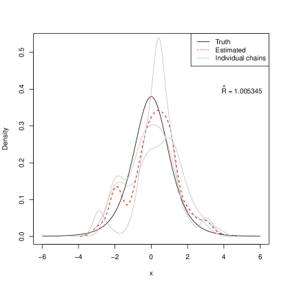
Figure 1: Density estimate and $\hat{R}$ along with the three individual density estimates.

The termination threshold critically impacts the quality of estimation, yet current practices do not suffice. The suggested threshold of 1.1 seems arbitrary and—as the example suggests—may be much too high to yield confidence in final estimates. We respond with two contributions: (i) we present an improved GR statistic and (ii) we establish a principled method of selecting a GR diagnostic termination threshold.

First, we propose improving both the univariate GR statistic (Section 3) and the multivariate GR statistic of Brooks and Gelman, (1998) (Section 4) by using recently-developed estimators of the variance of Monte Carlo averages. The relative efficiency of the original estimator used in the GR statistic versus our new estimator grows without bound as the chain length increases, resulting in dramatic stabilization of the GR statistic. Such an improvement was indirectly implied by Flegal et al., (2008).

Second, in Section 5, we present a method of selecting a principled, interpretable GR statistic cutoff by identifying a one-to-one correspondence between the GR statistic and the effective sample size (ESS) for estimating the mean of the target distribution. Specifically, we show that

$$\hat{R}\approx\sqrt{1+\dfrac{m}{\text{ESS}}}\,.$$

Thus, for $m$ chains, choosing a termination threshold $1.1$ implies an ESS of approximately $5m$, or five independent samples per chain; this is clearly too low to estimate the mean with any reasonable certainty.

In Section 6, we assess the performance of our methods in four examples. First, we present a complete analysis of the $t_{5}$-distribution example. The second example uses an autoregressive model—for which underlying true variances are known—to assess the two statistics’ time-to-convergence stability as it compares to the truth. The third example compares the traditional and updated GR statistics’ performance for a bimodal target distribution. We consider two cases, the first when the Markov chain gets stuck in a local mode, and the second when the Markov chain is able to jump between modes. The fourth and final example demonstrates the implementation of our improved GR statistic on a Bayesian logistic regression model analyzing the Titanic dataset; this highlights the marked improvement in the regression estimates’ stability when using the ESS-based termination threshold. We end with a discussion in Section 7.

2 Markov chains and convergence

Let $F$ be a target distribution defined on a space $\mathsf{X}$ equipped with a countably generated $\sigma$-field, $\mathcal{B}(\mathsf{X})$. Let $P:\mathsf{X}\times\mathcal{B}(\mathsf{X})\to[0,1]$ denote a Markov chain transition kernel such that for $x\in\mathsf{X}$ and $A\in\mathcal{B}(\mathsf{X})$, $P(x,A)=\Pr(X_{2}\in A|X_{1}=x)$. For $i=1,\dots,m$, let $\{X_{it}\}_{t\geq 1}$ denote the $i$th independent Markov chain. The starting value of the Markov chains, $X_{i1}$, are user-chosen and are either fixed or drawn randomly from a convenient initial distribution. We assume that $P$ is $F$-invariant and Harris ergodic (see Meyn and Tweedie,, 2009, for definitions) for definitions so that $P$ converges to $F$ (in total variation distance) for any initial distribution.

Typically, MCMC returns samples that are correlated and only approximately from $F$. This has allowed for diverse literature on the issue of convergence of an MCMC algorithm. There are two main types of convergence that are relevant to most MCMC problems (see Roy,, 2020; Vats et al.,, 2020, for a detailed discussion): (i) the convergence of the $n$-step Markov transition, $P^{n}$, to the stationary distribution $F$, and (ii) the convergence of sample statistics to the truth. The first is often termed as the “burn-in” problem, where a first chunk of the samples is discarded when the starting distribution of $X_{i1}$ is far away from $F$. Determining how many samples to retain is a challenging problem that often involves a detailed study of the specific Markov chain kernel, $P$. See Rosenthal, (1995); Jones and Hobert, (2001) for a theoretical exposition.

Convergence diagnostics that address the second class of convergence either assess convergence of the empirical distribution function or assess convergence of moments of functions of interest. Many density-based diagnostics have been proposed in the literature. Boone et al., (2014) measure the Hellinger distance between estimated marginal densities from multiple chains. A similar approach was used by Hjorth and Vadeby, (2005) with a distance metric similar to the Kullback Leibler (KL) divergence and by Dixit and Roy, (2017) with a KL divergence and adaptive kernel density estimators. VanDerwerken and Schmidler, (2017) use a state-space partition of the clusters in the MCMC output to diagnose convergence of the estimated target distribution.

This article and the original Gelman-Rubin diagnostic focuses on diagnosing moment-based convergence. That is, if interest is in estimating the mean, quantile, variance, etc of $F$, the MCMC process is said to have converged when the sample statistics are close enough to the truth. Convergence is guaranteed due to Harris ergodicity of the chains. Suppose interest is in estimating the mean of the posterior distribution $F$, $\mu=\text{E}_{F}X_{it}$. The Monte Carlo average of each chain estimates $\mu$ consistently. That is, as $n\to\infty$, due to the Markov chain strong law

$$\bar{X}_{i\cdot}=\dfrac{1}{n}\displaystyle\sum_{t=1}^{n}X_{it}\overset{a.s.}{\to}\mu\,.$$

The combined estimator of $\mu$ from the $m$ Markov chains is

$$\hat{\mu}=\dfrac{1}{m}\sum_{i=1}^{m}\bar{X}_{i\cdot}\overset{a.s.}{\to}\mu\,,$$

as $n\to\infty$. If $m=1$, then $\hat{\mu}=\bar{X}_{1\cdot}$. Moment-based diagnostic tools measure the quality of estimation of $\hat{\mu}$. Geweke, (1992) constructed a hypothesis test for testing the equality of the means of two nonoverlapping sections of a Markov chain. These sections are usually the first 10% and the last 50% of the chain. Similarly, Raftery and Lewis, (1992) used a two-state Markov chain assumption to construct a univariate diagnostic based on estimating quantiles of univariate components of the target distribution. A comprehensive survey of these and other diagnostics can be found in Cowles and Carlin, (1996) which also extends the above to the case when interest is in estimating the mean of a function $g:\mathsf{X}\to\mathbb{R}^{p}$. Almost all of the methods require the estimation of the limiting variance $\tau^{2}_{\infty}:=\lim_{n\to\infty}n\text{Var}(\bar{X}_{i\cdot})$, which is finite if a Markov chain central limit theorem holds (see Jones,, 2004, for conditions). That is, a Markov chain central limit theorem holds if there exists $\tau^{2}_{\infty}<\infty$ such that as $n\to\infty$

$$\sqrt{n}(\bar{X}_{i\cdot}-\mu)\overset{d}{\to}N(0,\tau^{2}_{\infty})\,.$$ (1)

Flegal and Gong, (2015); Gong and Flegal, (2016); Jones et al., (2006) propose a family of sequential termination rules that stop simulation the first time the variability in $\hat{\mu}$ is (relatively) small. For the sequential stopping rules to yield confidence regions with the nominal coverage probability, estimators of $\tau^{2}_{\infty}$ must be strongly consistent, a property that has been shown for a wide range of estimators, including batch means (Liu and Flegal,, 2018; Vats et al.,, 2019), spectral variance (Flegal and Jones,, 2010; Vats et al.,, 2018) and regeneration-based estimators (Jones et al.,, 2006; Seila,, 1982).

By far, the most popular method for terminating an MCMC sampler run is the Gelman-Rubin diagnostic of Gelman and Rubin, (1992) and Brooks and Gelman, (1998). In the following sections, we introduce the Gelman-Rubin diagnostic in detail and reformulate the univariate and multivariate diagnostics facilitating the use of strongly consistent estimators of $\tau^{2}_{\infty}$. This allows us to find a novel connection between ESS and the Gelman-Rubin statistic, thus motivating a termination threshold for the Gelman-Rubin statistic. As in Gelman and Rubin, (1992), we assume throughout that a Markov chain central limit theorem holds.

3 Univariate diagnostic

3.1 Original Gelman-Rubin statistic

Let $F$ be the target distribution with mean $\mu\in\mathbb{R}$ and variance $\sigma^{2}<\infty$. Gelman and Rubin, (1992) construct two estimators of $\sigma^{2}$ and compare the square root of their ratio to 1. This process is described below.

Recall that $\bar{X}_{i\cdot}$ is the sample mean from chain $i$ and $\hat{\mu}$ is the overall mean. Let $s_{i}^{2}$ denote the sample variance for chain $i$ and $s^{2}$ be the average of the $m$ sample variances. That is,

$$s_{i}^{2}=\dfrac{1}{n-1}\sum_{t=1}^{n}(X_{it}-\bar{X}_{i\cdot})^{2}\qquad\text{ and }\qquad s^{2}=\dfrac{1}{m}\sum_{i=1}^{m}s_{i}^{2}\,.$$

Although $s^{2}$ is strongly consistent for $\sigma^{2}$ as $n\to\infty$, it is biased for $\sigma^{2}$ for non-trivial Markov chains. In fact,

$$\text{E}_{F}(s_{i}^{2})=\dfrac{n}{n-1}\left(\sigma^{2}-\text{Var}_{F}(\bar{X}_{i\cdot})\right)\,.$$ (2)

When the samples are independent and identically distributed, $\text{Var}_{F}(\bar{X}_{i\cdot})=\sigma^{2}/n$ and $s_{i}^{2}$ is an unbiased estimator of $\sigma^{2}$. However, for samples obtained through MCMC, $\text{Var}_{F}(\bar{X}_{i\cdot})$ is often much larger than $\sigma^{2}/n$ due to positive correlation in the Markov chain. Thus, $s_{i}^{2}$ on average, underestimates the target variance.

Define $\tau^{2}_{n}:=n\text{Var}_{F}(\bar{X}_{i\cdot})$ and let $\tau^{2}_{\infty}=\lim_{n\to\infty}\tau^{2}_{n}<\infty$. Gelman and Rubin, (1992) perform a bias correction by estimating $\tau^{2}_{n}/n=\text{Var}_{F}(\bar{X}_{i\cdot})$ with $B$, the sample variance of sample means from $m$ chains. That is,

$$\dfrac{B}{n}=\dfrac{1}{m-1}\displaystyle\sum_{i=1}^{m}(\bar{X}_{i\cdot}-\hat{\mu})^{2}\,.$$ (3)

Using (3) to estimate $\text{Var}_{F}(\bar{X}_{i\cdot})$ in (2) yields the following estimator of $\sigma^{2}$:

$$\hat{\sigma}^{2}:=\dfrac{n-1}{n}s^{2}+\dfrac{B}{n}\,.$$

The univariate GR potential scale reduction factor (PSRF) is

$$\hat{R}=\sqrt{\dfrac{\hat{\sigma}^{2}}{s^{2}}}\,.$$ (4)

Gelman and Rubin, (1992) and Gelman et al., (2004) argue that if an over-dispersed starting distribution for the Markov chain is used, $\hat{\sigma}^{2}$ overestimates $\sigma^{2}$—due to (2)—and $s^{2}$ underestimates $\sigma^{2}$. Since both are consistent for $\sigma^{2}$, $\hat{R}$ decreases to 1 as $n$ increases. Simulation is stopped when $\hat{R}\leq\delta$ for some $\delta>1$.

Remark 1.

The univariate PSRF presented by Brooks and Gelman, (1998) and Gelman and Rubin, (1992) differs from (4). Specifically, it is defined as

$$\sqrt{\hat{R}}=\sqrt{\dfrac{\hat{\sigma}^{2}+\frac{B}{mn}}{s^{2}}\dfrac{df+3}{df+1}}\,,$$

where $df$ is the degrees of freedom for the numerator estimated via a method of moments. Since this original estimator, $\hat{R}$ has evolved into the expression in (4). Popular resources for MCMC convergence diagnostics such as Gelman et al., (2004) and softwares such as Stan use the expression in (4). Although the R package coda uses the original GR expression, we commit to the expression in (4).

3.2 New univariate PSRF

Our improved construction of the PSRF incorporates efficient estimators of $\text{Var}_{F}(\bar{X}_{i\cdot})$. Due to the correlation in the Markov chain,

$$\tau^{2}_{n}=n\text{Var}_{F}\left(\bar{X}_{i\cdot}\right)=\text{Var}_{F}(X_{i1})+2\sum_{k=1}^{n-1}\left(\dfrac{n-k}{n}\right)\text{Cov}_{F}\left(X_{i1},X_{i(1+k)}\right)\,.$$

We use known estimators of $\tau^{2}_{\infty}$ to estimate $\tau^{2}_{n}$; in fact these estimators are technically estimating $\tau^{2}_{n}$ but are consistent for $\tau^{2}_{\infty}$ as $n\to\infty$. A significant amount of research in the past two decades has resulted in improved estimation of $\tau^{2}_{\infty}$. This includes batch means estimators and regenerative estimators (Jones et al.,, 2006), spectral variance estimators and overlapping batch means estimators (Flegal and Jones,, 2010), and weighted batch means estimators (Liu and Flegal,, 2018). Under appropriate conditions, the estimators above are strongly consistent but are biased from below for $\tau^{2}_{\infty}$ (Vats and Flegal,, 2018). The initial sequence estimators of Geyer, (1992) are asymptotically conservative but only apply to reversible Markov chains.

We use a lugsail version of the replicated batch means estimator to estimate $\tau^{2}_{n}$. As Vats and Flegal, (2018) describe, the lugsail estimator is biased from above in finite samples but strongly and mean square consistent for $\tau^{2}_{\infty}$ as $n\to\infty$. Thus, even without an over-dispersed starting distribution, the lugsail estimator yields a biased-from-above estimate of $\tau^{2}_{n}$. In order to combine variance estimates from multiple chains, we use a replicated version of the lugsail batch means estimator à la Argon and Andradóttir, (2006). This replicated estimator accounts for the case when independent copies of the chain are concentrated in different areas of the support of the distribution, a case that arises often in multi-modal targets. We now describe the replicated lugsail batch means estimator.

Suppose $n$ is such that $n=a\cdot b$ where $a$ is the number of batches and $b$ is the batch size. Both $a$ and $b$ must increase with $n$; usual choices of $b$ include $\lfloor n^{1/3}\rfloor$ and $\lfloor n^{1/2}\rfloor$. For the $i$th chain, define the mean for batch $k=1,\dots,a$ as

$$\bar{Y}_{ik}=\dfrac{1}{b}\sum_{t=(k-1)b+1}^{kb}X_{it}\,.$$

The replicated batch means estimator of $\tau^{2}_{n}$ is,

$$\hat{\tau}_{b}^{2}:=\dfrac{b}{am-1}\displaystyle\sum_{i=1}^{m}\sum_{k=1}^{a}(\bar{Y}_{ik}-\hat{\mu})^{2}\,.$$

Here the subscript $b$ in $\hat{\tau}_{b}^{2}$ indicates the batch size used to construct the estimator. The replicated lugsail batch means estimator is,

$$\hat{\tau}^{2}_{L}:=2\hat{\tau}_{b}^{2}-\hat{\tau}_{b/3}^{2}\,,$$ (5)

where $\hat{\tau}_{b/3}^{2}$ is the replicated batch means estimator constructed using batch size $\lfloor b/3\rfloor$.

An advantage of $\hat{\tau}^{2}_{L}$ over $B$ is its relative efficiency. The large sample variance of $B$ is $2\tau^{4}_{\infty}/(m-1)$ (Gelman and Rubin,, 1992) while the large-sample variance of the replicated lugsail batch means estimator is $6\tau^{4}_{\infty}/am$ (Gupta and Vats,, 2020; Argon and Andradóttir,, 2006). Because $a$ increases with $n$, the large sample relative efficiency of $B$ versus $\hat{\tau}^{2}_{L}$ is

$$\text{eff}(B,\hat{\tau}^{2}_{L})=\dfrac{ma}{3(m-1)}\to\infty\qquad\text{ as }n\to\infty\,.$$ (6)

Equation (6) shows that as the Markov chain length increases, the relative variance of $B$ versus $\hat{\tau}^{2}_{L}$ grows; for any reasonable choice of $n$, the replicated lugsail batch means estimator is markedly more efficient than $B$. Section 6 will show that incorporating $\hat{\tau}^{2}_{L}$ rather than $B$ dramatically stabilizes the termination of MCMC.

Using $\hat{\tau}^{2}_{L}$ instead of $B$ yields the following biased-from-above estimator of $\sigma^{2}$

$$\hat{\sigma}^{2}_{L}:=\dfrac{n-1}{n}s^{2}+\dfrac{\hat{\tau}_{L}^{2}}{n}\,.$$

Using $\hat{\sigma}^{2}_{L}$ instead of $\hat{\sigma}^{2}$ in $\hat{R}$ yields the following improved estimator for the PSRF:

$$\hat{R}_{L}=\sqrt{\dfrac{\hat{\sigma}^{2}_{L}}{s^{2}}}\,.$$ (7)

As before, the criterion for terminating simulation is $\hat{R}_{L}\leq\delta$ for some $\delta>1$.

4 Multivariate PSRF

4.1 Original multivariate PSRF

Most MCMC problems are inherently multivariate in that the goal is to sample from a multidimensional target distribution. Acknowledging the multivariate nature of estimation is critical in order to account for the interdependence between components of the chain (Vats et al.,, 2019). Brooks and Gelman, (1998) proposed the following multivariate extension of the univariate GR diagnostic.

Let $F$ be a $p$-dimensional target distribution with mean $\mathbf{\mu}\in{\mathbb{R}}^{p}$ and let $\Sigma$ be the $p\times p$ variance-covariance matrix of the target distribution. Let $\mathbf{X}_{i1},\dots,\mathbf{X}_{in}$ be the $i$th parallel Markov chain; each $\mathbf{X}_{it}=(X_{it1},\dots,X_{itp})^{T}\in{\mathbb{R}}^{p}$. Let $\bar{\mathbf{X}}_{i\cdot}=n^{-1}\sum_{t=1}^{n}\mathbf{X}_{it}$ be the mean vector of the $i$th chain and let the overall mean be $\hat{\mathbf{\mu}}=m^{-1}\sum_{i=1}^{m}\bar{\mathbf{X}}_{i\cdot}$. Let $S_{i}$ be the sample covariance matrix for chain $i$, and let $S$ be the sample mean of $S_{1},\ldots,S_{m}$. That is

$$S_{i}=\dfrac{1}{n-1}\displaystyle\sum_{t=1}^{n}(\mathbf{X}_{it}-\bar{\mathbf{X}}_{i\cdot})(\mathbf{X}_{it}-\bar{\mathbf{X}}_{i\cdot})^{T}\qquad\text{ and }\qquad S=\dfrac{1}{m}\sum_{i=1}^{m}S_{i}\,.$$

Just as in the univariate case, Brooks and Gelman, (1998) decompose the target variance:

$$\Sigma=\left(\dfrac{n-1}{n}\right)\text{E}_{F}(S)+\text{Var}_{F}(\bar{\mathbf{X}}_{i\cdot})\,.$$

Let $T_{n}:=n\text{Var}_{F}(\mathbf{\bar{X}}_{i\cdot})$ and let $T_{\infty}=\lim_{n\to\infty}n\text{Var}_{F}(\mathbf{\bar{X}}_{i\cdot})$. Then $T_{\infty}$ is the asymptotic variance-covariance matrix in the multivariate Markov chain CLT. When $p=1$, $T_{n}=\tau^{2}_{n}$ and $T_{\infty}=\tau^{2}_{\infty}$. Brooks and Gelman, (1998) estimate $T_{n}/n$ with the sample covariance matrix of the sample mean vectors from $m$ chains. Define $\mathbf{B}$ such that

$$\dfrac{\mathbf{B}}{n}=\dfrac{1}{m-1}\sum_{i=1}^{m}(\mathbf{\bar{X}}_{i\cdot}-\mathbf{\hat{\mu}})(\mathbf{\bar{X}}_{i\cdot}-\mathbf{\hat{\mu}})^{T}\,.$$

Using $\mathbf{B}/n$ to correct for the bias in $S$ yields

$$\widehat{\Sigma}:=\left(\dfrac{n-1}{n}\right)S+\dfrac{\mathbf{B}}{n}\,.$$

As in the univariate case, the goal is to compare the ratio of these estimators of $\Sigma$. However, because $\Sigma$ is a $p\times p$ matrix, a univariate quantification of this ratio is required. Let $\lambda_{\max}(A)$ denote the largest eigenvalue of a matrix $A$. The multivariate PSRF is

$$\hat{R}^{p}=\sqrt{\left(\dfrac{n-1}{n}\right)+\dfrac{\lambda_{\max}(S^{-1}\mathbf{B})}{n}}\,.$$ (8)

Remark 2.

As in the univariate case, we use a different expression from the original paper by Brooks and Gelman, (1998) so that the multivariate expression here is a direct generalization of the univariate PSRF. The expression in Brooks and Gelman, (1998) is

$$\hat{R}^{p}=\sqrt{\left(\dfrac{n-1}{n}\right)+\left(\dfrac{m+1}{m}\right)\dfrac{\lambda_{\max}(S^{-1}\mathbf{B})}{n}}\,.$$

The estimator $\mathbf{B}$ will not be positive definite in the realistic event of $m$ being smaller than $p$. Also, the use of the largest eigenvalue is likely the reason the multivariate PSRF has not found large practical use in the literature. The largest eigenvalue quantifies the variability in the direction of the largest variation, the principal eigenvector of $S^{-1}\mathbf{B}$. This can be significantly larger than any of the individual variances, thus leading to a needlessly conservative termination criterion.

4.2 New multivariate PSRF

Recent work by Dai and Jones, (2017), Kosorok, (2000), Liu and Flegal, (2018), Vats and Flegal, (2018), and Vats et al., (2018) provide estimators of $T_{\infty}$. We use the biased-from-above, multivariate replicated lugsail batch means estimator to estimate $T_{n}$. As before, for the $i$th chain, define the mean vector for batch $k=1,\dots,a$ as

$$\bar{\mathbf{Y}}_{ik}=\dfrac{1}{b}\sum_{t=(k-1)b+1}^{kb}\mathbf{X}_{it}\,.$$

The multivariate replicated batch means estimator of $T_{n}$ is,

$$\hat{T}_{b}:=\dfrac{b}{am-1}\displaystyle\sum_{i=1}^{m}\sum_{k=1}^{a}(\bar{\mathbf{Y}}_{ik}-\hat{\mu})(\bar{\mathbf{Y}}_{ik}-\hat{\mu})^{T}\,.$$

The multivariate replicated lugsail batch means estimator for the $i$th chain is,

$$\hat{T}_{L}:=2\hat{T}_{b}-\hat{T}_{b/3}\,.$$ (9)

Define

$$\hat{\Sigma}_{L}=\left(\dfrac{n-1}{n}\right)S+\dfrac{\hat{T}_{L}}{n}\,.$$

Let $\det(\cdot)$ denote determinant. We define our multivariate PSRF as

$$\hat{R}^{p}_{L}=\sqrt{\left(\dfrac{n-1}{n}\right)+\dfrac{\det(S^{-1}\hat{T}_{L})^{1/p}}{n}}\,.$$ (10)

Remark 3.

We use the function $\det(\cdot)^{1/p}$ instead of the largest eigenvalue for multiple reasons. First, note that

$$\det(S^{-1}\hat{T}_{L})^{1/p}=\left(\dfrac{\det(\hat{T}_{L})}{\det(S)}\right)^{1/p}\,.$$

Since the determinant of a covariance matrix of a random variable is referred to as the generalized variance of the random variable (Wilks,, 1932), this ratio of generalized variances is akin to the ratio of variances in the univariate case. Second, the $p$th root of the determinant is the geometric mean of the eigenvalues of the matrix. Thus, the determinant accounts for variability in all directions and not only in the direction of the principal eigenvector. The power $1/p$ ensures stability and invariance to change of units (SenGupta,, 1987). Also, when $p=1$, (10) is the univariate PSRF in (7).

Remark 4.

Users commonly run a single Markov chain in their analysis ($m=1$). The use of the replicated lugsail batch means estimators to estimate $T_{\infty}$ or $\tau^{2}_{\infty}$ allows a direct application of the GR statistic to a single chain.

5 Relation to ESS and choosing $\delta$

A challenge in implementing the GR diagnostic is choosing the PSRF cutoff, $\delta$. Gelman et al., (2004), say

The condition of $\hat{R}$ near 1 depends on the problem at hand; for most examples, values below 1.1 are acceptable, but for a final analysis in a critical problem, a higher level of precision may be required.

In this section we establish and highlight the relationship between ESS and PSRF. Using the quantitative guidelines established in the literature for terminating simulation using ESS, we obtain interpretable values of $\delta$.

For an estimator, ESS is the number of independent samples with the same standard error as a correlated sample. Recall that $T_{\infty}$ is the covariance matrix in the Markov chain CLT and $\Sigma$ is the covariance matrix of the target distribution. If $p=1$, both $T_{\infty}$ and $\Sigma$ are scalars. For $m\geq 1$ chains, each of length $n$, Vats et al., (2019) define ESS as

$$\text{ESS}=mn\left(\dfrac{\det(\Sigma)}{\det(T_{\infty})}\right)^{1/p}\,.$$

For $p=1$, this reduces to the following univariate definition of ESS as discussed by Gong and Flegal, (2016) and Kass et al., (1998):

$$\text{ESS}_{p=1}=mn\dfrac{\sigma^{2}}{\tau^{2}_{\infty}}\,.$$

Strongly consistent estimators of $T_{\infty}$ and $\Sigma$ will yield a strongly consistent estimator of ESS. Thus, an estimator of ESS is the following:

$$\widehat{\text{ESS}}=mn\left(\dfrac{\det(\hat{S})}{\det(\hat{T}_{L})}\right)^{1/p}\,\,.$$

A theoretically-justified lower bound on the number of effective samples required to obtain a certain level of precision has been determined for the univariate case (Gong and Flegal,, 2016) and for the general multivariate problem (Vats et al.,, 2019). Just as we can calculate the sample size necessary to construct a confidence interval with a desired width, we can obtain a lower bound on the ESS necessary to construct a confidence region with a desired relative volume. Suppose the goal is to make $100(1-\alpha)\%$ confidence regions for $\mu$, using estimator $\hat{\mu}$. Let $\epsilon$ be the desired volume of the confidence region for $\hat{\mu}$ relative to the generalized standard deviation in the target distribution, $\det(\Sigma)^{1/2p}$. Then $\epsilon$—the relative volume of the confidence region—is akin to the width of a confidence interval in sample size calculations.

Let $\chi^{2}_{1-\alpha,p}$ be the $(1-\alpha)$th quantile of the $\chi^{2}$ distribution with $p$ degrees of freedom. Vats et al., (2019) show that if simulation is terminated when the estimated ESS satisfies

$$\widehat{\text{ESS}}\geq\dfrac{(2)^{2/p}\pi}{(p\Gamma(p/2))^{2/p}}\dfrac{\chi^{2}_{1-\alpha,p}}{\epsilon^{2}}:=M_{\alpha,\epsilon,p}\,,$$ (11)

then the confidence regions created at termination will asymptotically have the correct coverage probability. The lower bound $M_{\alpha,\epsilon,p}$ can be calculated a priori, and simulation can terminate when the estimated ESS exceeds $M_{\alpha,\epsilon,p}$.

It is straightforward to see that

$$\hat{R}^{p}_{L} =\sqrt{\left(\dfrac{n-1}{n}\right)+\dfrac{m}{\widehat{\text{ESS}}}}$$

$$\approx\sqrt{1+\dfrac{m}{\widehat{\text{ESS}}}}$$

$$\leq\sqrt{1+\dfrac{m}{M_{\alpha,\epsilon,p}}}:=\delta_{\epsilon}\,.$$ (12)

Because $\delta_{\epsilon}$ can be calculated a priori, simulation can terminate when the PSRF drops below the threshold $\delta_{\epsilon}$. The value of $M_{\alpha,\epsilon,p}$ is obtained from (11) and is most affected by the choice of $\epsilon$ (Vats et al.,, 2019). Therefore, the desired $\delta_{\epsilon}$ will be most affected by the choice of $\epsilon$. Because $\epsilon$ is interpretable, $\delta_{\epsilon}$ is interpretable; terminating when $\hat{R}^{p}_{L}\leq\delta_{\epsilon}$ is equivalent to terminating simulations when $\widehat{\text{ESS}}\geq M_{\alpha,\epsilon,p}$ for estimating the mean of the target distribution.

Example 1.

In our examples, we choose $\epsilon=.10$ and $\alpha=.05$. That is, for creating 95% confidence regions, we desire the volume of the confidence region for the Monte Carlo estimator of the mean to be less than 10% of $\det(\Sigma)^{1/2p}$. For problems with $m=3$ and $p=1$, $M_{.05,.10,1}=1537$, which corresponds to $\delta_{\epsilon}=1.000976$. Thus, the desired termination threshold in this situation is dramatically lower than the ad-hoc cutoff of 1.1.

Remark 5.

Vats et al., (2019) explain that a minimum simulation effort must be set to safeguard from premature termination due to early bad estimates of $\sigma^{2}$. We concur and suggest a minimum simulation effort of $n=M_{\alpha,\epsilon,p}$.

6 Examples

6.1 $t_{5}$-distribution continued

Recall the $t_{5}$-distribution example introduced in Section 1, where we run $m=3$ chains with starting values randomly sampled from a $t_{2}$-distribution. For our seed, the starting points were $(0.484,1.370,-0.131)$. For $\delta=1.1,\delta=1.01$, and $\delta_{.1}=1.000975$, we check whether each convergence criterion is satisfied for $\hat{R}_{L}$ in increments of 50 iterations and present the estimated density plots in Figure 2. For $\delta=1.1$ and $\delta=1.01$, the termination criteria are met at $n=50$. The density estimate clearly indicates poor quality of estimation. For $\delta_{.1}=1.000975$, the sampler terminates at $n=2350$ iterations, resulting in improved estimation. Further smaller values of $\epsilon$ will provide further improvements, and $\epsilon$ can be chosen based on the quality of estimation desired. In Figure 2, we also present a running plot of $\hat{R}$ and $\hat{R}_{L}$ which illustrates the erratic behavior of $\hat{R}$, especially for small sample sizes. In comparison, $\hat{R}_{L}$ is far more stable and exhibits monotonic decreasing behavior (up to randomness).

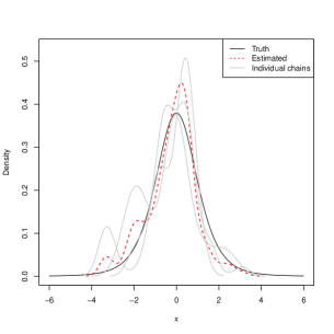
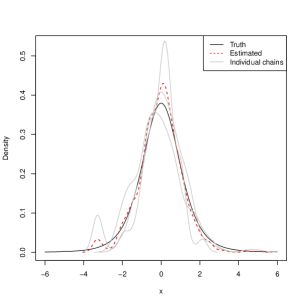
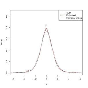
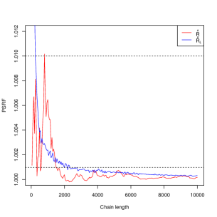
Figure 2: $t$-distribution: (From left to right and top to bottom). Estimated density using $\hat{R}_{L}$ with $\delta=1.1$, $\delta=1.01$ and $\delta_{.1}=1.000975$. Bottom right is a running plot of the estimated PSRF using both $\hat{R}$ (red) and $\hat{R}_{L}$ (blue). The horizontal dotted black line is $\delta_{.1}=1.000975$.

6.2 Autoregressive process of order 1

Consider the autoregressive process of order 1 (AR(1)). For $t=1,2,\dots$, let $Y_{t}\in{\mathbb{R}}$ and $\epsilon_{t}\sim N(0,\nu^{2})$. For $|\rho|<1$, the AR(1) process is

$$Y_{t}=\rho Y_{t-1}+\epsilon_{t}\,.$$

This describes a Markov chain with stationary distribution $N(0,\sigma^{2})$, where

$$\sigma^{2}=\dfrac{\nu^{2}}{1-\rho^{2}}\,.$$ (13)

The autocorrelation coefficient $\rho$ determines the rate of convergence of the Markov chain. In particular, if $|\rho|<1$ a Markov chain CLT holds for $\bar{Y}_{n}=n^{-1}\sum_{t=1}^{n}Y_{t}$ with the following asymptotic variance:

$$\tau^{2}_{\infty}=\sigma^{2}\;\dfrac{1+\rho}{1-\rho}\,.$$

For finite $n$, we can obtain an expression for $\tau^{2}_{n}=n\text{Var}_{F}(\bar{Y}_{n})$,

$$\tau^{2}_{n} =\sigma^{2}+2\sigma^{2}\sum_{k=1}^{n-1}\left(\dfrac{n-k}{n}\right)\rho^{k}\,.$$ (14)

In this example, we set $\nu=1$ and $\rho=.95$. Since the true values of $\tau^{2}_{n}$ and $\sigma^{2}$ are known, we can compare the performance of our proposed methods with that of the original GR methods. Over 500 replications, we determine when $\hat{R}$ and $\hat{R}_{L}$ reach $\delta$ and record the Monte Carlo estimate, $\bar{Y}_{n}$, and termination sample size; each criterion is checked in increments of 500 iterations. In Figure 3, we plot $\bar{Y}_{n}$ at termination versus the termination index using both $\hat{R}$ and $\hat{R}_{L}$ for a single chain and for $m=5$ chains. For these simulations, we set $\epsilon={.10}$ and use $m=5$; this yields termination threshold $\delta_{\epsilon}=1.001625$. We compare our results against the true value of the PSRF determined by (13) and (14).

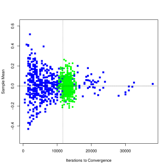
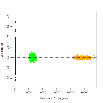
Figure 3: AR(1): Sample mean versus termination iteration for $m=5$ chains. (Left) Blue squares are for $\hat{R}$; green points are for $\hat{R}_{L}$. The horizontal dotted line is the true mean. The vertical dotted line is the true chain length for termination cutoff $\delta_{.10}$. (Right) Blue squares are for $\hat{R}_{L}\leq\delta=1.1$. Green points and orange triangles are for $\hat{R}_{L}\leq\delta_{.10}$ and $\hat{R}_{L}\leq\delta_{.05}$, respectively. The horizontal dotted line is the true mean.

In Figure 3, we present our simulation results. First, we inspect the horizontal variability by comparing the number of iterations required for convergence for the two convergence statistics. The variability in the termination procedure using $\hat{R}$ is large: some runs converged almost immediately while others required over 30,000 steps. The replicated lugsail batch means estimators terminate close to the true termination index and do so with considerably lower variability; this follows from the efficiency result in (6). Second, we inspect the vertical variability in Figure 3: the means produced at termination by $\hat{R}_{L}$ have low, near-uniform variability in each plot while the original GR diagnostic produces means with more variability.

Unlike $\hat{R}$, $\hat{R}_{L}$ can be calculated for a single chain. In Figure 4, we plot the iterations to convergence for $\hat{R}_{L}$ using three convergence criteria versus the estimated sample mean at convergence. The plot here is essentially similar to the right plot in Figure 3 in that it is clear that $\delta=1.1$ yields high variability in the resulting estimates.

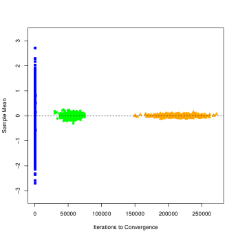
Figure 4: AR(1): Sample mean versus termination iteration for $m=1$ chain. Blue squares are for $\hat{R}_{L}\leq\delta=1.1$. Green points and orange triangles are for $\hat{R}_{L}\leq\delta_{.10}$ and $\hat{R}_{L}\leq\delta_{.05}$, respectively. The horizontal dotted line is the true mean.

For three different termination criteria we calculate the iterations to convergence using $\hat{R}_{L}$ and the Monte Carlo average at convergence. Results are in the right plot of Figure 3. Naturally, smaller values of $\epsilon$—which correspond to smaller values of $\delta_{\epsilon}$—yield later termination. Most importantly, we note the poor performance of the ad-hoc $\hat{R}_{L}\leq 1.1$ criterion: the variability in the sample mean is much too large to yield any confidence in the quality of estimation.

6.3 Bimodal Gaussian distribution

Let $f(x;\theta,\lambda^{2})$ be the density of a normal distribution with mean $\theta$ and variance $\lambda^{2}$. Consider the following density of a mixture distribution of two normal random variables:

$$f(x)=\dfrac{1}{2}f_{1}(x;0,2)+\dfrac{1}{2}f_{2}(x;10,.5)\,.$$

We run a random walk Metropolis-Hastings MCMC algorithm with proposal distribution $N(\cdot,h)$ and consider two choices of $h$: $h=1$ and $h=10$. A larger $h$ allows the Markov chains to jump between modes relatively easily so that each Markov chain explores the state space relatively well. The first setting with $h=1$ localizes each Markov chain, not allowing them to easily jump modes. Trace plots illustrating this behavior are in Figure 5.

Figure 5: Bimodal: Trace plots of one Markov chain run for $h=1$ (left) and $h=10$ (right).

For $h=1$, we run $m=5$ Markov chains from the first mode and track both $\hat{R}$ and $\hat{R}_{L}$. Since the Markov chains do not adequately explore the state space—in particular, the chains have not discovered the second mode yet—both methods prematurely diagnose convergence; see Figure 6 where the Markov chains satisfy $\hat{R}_{L}<\delta_{.1}=1.001625$ at $n=4100$. Since this declaration of convergence is premature, the estimated density plot at termination is nowhere near the truth. The GR diagnostic, even with our improvements, cannot possibly detect lack of convergence when the chain has failed to travel to areas of critical mass. It is thus imperative to choose an MCMC sampler that adequately explores the state space before any output analysis is considered.

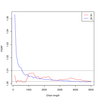
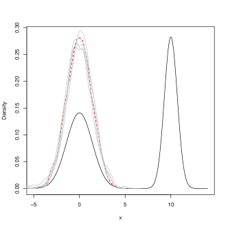
Figure 6: Bimodal: Running plot of PSRF estimates with horizontal lines drawn at $\delta=1.01$ and $\delta_{.1}=1.001625$ (left) and estimated density plot at termination using $\hat{R}_{L}\leq\delta_{.1}$ (right).

For $h=10$, the Markov chain is able to move across modes often so that sample quantities are well estimated. Over 500 replications, we run $m=5$ Markov chains starting from an over-dispersed distribution. In each replication, we record the chain length at $\hat{R}\leq\delta_{.1}$ and $\hat{R}_{L}\leq\delta_{.1}$. Results are presented in the left plot of Figure 7. Using $\hat{R}$ results in termination as early as chain length 500 and as late as chain length 1.5e5. In contrast, $\hat{R}_{L}$ has far less variability in the termination time and in the sample mean estimates at termination.

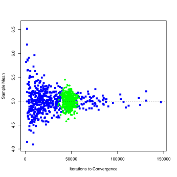
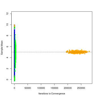
Figure 7: Bimodal: Sample mean versus Monte Carlo sample size at termination with the horizontal dotted line being the true mean. (Left) For $m=5$ chains with termination threshold $\delta_{.1}$. Blue squares are obtained using $\hat{R}$; green points are obtained using $\hat{R}_{L}$. (Right) For $m=1$ chain with statistic $\hat{R}_{L}$ and three termination thresholds. Blue squares are obtained using $\delta=1.1$, green points are obtained using $\delta=1.01$, and orange triangles are obtained using $\delta_{.1}$.

In order to assess the performance of $\hat{R}_{L}$ for a single chain, we implemented another simulation study using only $\hat{R}_{L}$ for $m=1$ chain with cutoffs $\delta=1.1$, $\delta=1.01$, and $\delta_{.1}=1.000325$; the results are presented in the right plot of Figure 7. Barring two of the 500 replications where the single chain was not able to jump from the local mode, termination criterion $\delta_{.1}$ dramatically stabilizes the estimation quality at termination. The convergence criteria of $\delta=1.1$ and $\delta=1.01$ lead to premature termination.

6.4 Bayesian logistic regression: Titanic data

On April 15, 1912, the RMS Titanic sank after colliding with an iceberg on its maiden voyage. The accident killed 1502 of the 2224 passengers and crew on board. The titanic_train data in the R package titanic contains information on 891 passengers aboard the Titanic and whether they survived the tragedy or not. Additional information includes the class of the passenger (Pclass, a factor with three levels), sex (a factor with two levels), age, the number of siblings/spouses aboard (SibSp), the number of parents/children aboard (Parch), the passenger’s fare (Fare), and port of embarkation (Embarked, a factor with three levels). The data-set contains 179 entries with missing values, which we remove, yielding 712 observations.

We fit a Bayesian logistic regression model to this data. Let $Y_{1},\dots,Y_{712}$ be the observed binary response. $Y_{i}=1$ if the $i$th passenger survived and $Y_{i}=0$ otherwise. For $i=1,\dots,712$, let $x_{i}=(x_{i1},\dots,x_{i10})^{T}$ denote the vector of covariates for the $i$th response. For $\beta\in{\mathbb{R}}^{10}$, the Bayesian logistic regression setup is

$$Y_{i}\mid\beta\sim\text{Bernoulli}\left(\dfrac{1}{1+\exp(-x_{i}^{T}\beta)}\right)\,.$$

We assume a multivariate normal prior on $\beta$ (that is, $\beta\sim N(0,\sigma^{2}_{\beta}I_{10})$, where $I_{10}$ is the $10\times 10$ identity matrix). We set $\sigma^{2}_{\beta}=100$ to yield a diffuse prior on $\beta$. A random walk Metropolis-Hastings sampler available in the R package MCMCpack is used to sample from the intractable posterior. We tune the step size of the sampler to approximate the optimal acceptance probabilities indicated by Roberts et al., (1997).

Since posterior distribution is 10-dimensional, we employ the multivariate PSRF to determine the number of samples required. We run $m=5$ parallel chains with starting values from across -3 to 3 standard deviations from the maximum likelihood estimate of $\beta$. We start with $n=50$ and—as long as the multivariate PSRFs are above 1.1 and $\delta_{.10}$ in (12)—we increase the Markov chain length by 10%.

In 100 replications, we note the posterior mean of $\beta$ and the 95% credible interval at termination using both criteria. The results are in Figure 8. It is immediately clear that the ad-hoc threshold of $\delta=1.1$ yields credible intervals with unacceptably large variability, as illustrated by the left set of points in Figure 8; in this example, the $\delta=1.1$ cutoff yields untrustworthy estimates. In contrast, $\delta_{.10}$ produces credible interval estimates with minimal variability.

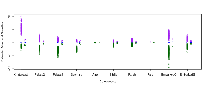
Figure 8: Titanic: Centered posterior mean and 95% credible interval estimates from 100 replications for all 10 components. Purple circles are upper quantiles, blue circles are posterior means, and green circles are lower quantiles. Each component has two sets of points: the left points are for $\hat{R}^{p}_{L}\leq 1.1$ and the right points are for $\hat{R}^{p}_{L}\leq\delta_{.10}$

Next we compare the performance of the multivariate PSRF using the determinant against the performance of the original multivariate PSRF in (8), which uses the largest eigenvalue (Brooks and Gelman,, 1998). In Figure 9, we track the evolution of the two statistics, along with the 10 univariate PSRFs, for one run of the 5 parallel chains. The determinant PSRF yields values close to the univariate PSRFs, but the largest eigenvalue PSRFs are markedly more conservative, resulting in delayed termination. If conservative termination is desirable, we recommend adhering to the determinant-based multivariate PSRF and using a smaller $\epsilon$ in order to retain the ESS interpretation of the procedure.

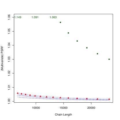
Figure 9: Titanic: Univariate PSRFs (blue dotted lines), multivariate PSRFs using the largest eigenvalue (green circles), and multivariate PSRFs using the determinant (red triangles) from $m=5$ parallel chains. Green text represents the PSRFs of circles that did not fit in the graph.

7 Discussion

The MCMC community has long held the view that the GR diagnostic is susceptible to premature and unreliable convergence diagnoses (Flegal et al.,, 2008). This certainly remains true in situations where the Markov chains are all stuck in a local mode (as demonstrated in Section 6.3). In this situation, we demonstrate the poor performance of $\delta=1.1$—as Vehtari et al., (2020) also acknowledged—and emphasize the importance of choosing a well-informed termination threshold. Even if the Markov chains explore different parts of the state space, we propose changes that strengthen the GR diagnostic in two significant ways: 1) we stabilize the GR statistic using improved estimators of Monte Carlo variance and 2) we safeguard against premature diagnosis by replacing $\delta=1.1$ with a principled, ESS-based termination threshold. Our diagnostic is available for public use in the R package stableGR (Knudson and Vats,, 2020).

To stabilize the GR statistic, we incorporate an efficient estimator of the variance of the Monte Carlo average: the replicated lugsail batch means estimator. Our examples demonstrate how this incorporation effectively stabilizes the time-to-convergence and the resulting sample means. An immediate advantage of the replicated lugsail batch means estimator is it can be calculated for a single chain; single chain output analysis has long been part of MCMC practice and our proposed GR statistic can easily assess convergence in this scenario. Ordinary batch means estimators and spectral variance estimators can also handle a single chain and might yield even higher statistical efficiency, but they do not naturally overestimate the Monte Carlo standard errors. This biased-from-above property of the lugsail estimator safeguards the statistic against early termination. Although we believe that the replicated lugsail batch means estimator is currently the best candidate for the GR statistic, univariate and multivariate Monte Carlo variance estimation is a rich, ongoing area of research: the GR statistic will benefit from continual adaptation to incorporate advances in this area.

To address premature convergence diagnoses, we inspect the PSRF threshold of 1.1. and through various example show that a premature convergence diagnosis is often due to the arbitrary PSRF threshold of 1.1. We establish a one-to-one mapping between PSRF and ESS and use this to show that a PSRF termination threshold of 1.1 yields approximately 5 effective samples per chain, which is far too small for any reasonable number of chains. We then leverage this ESS-PSRF connection to construct a principled, ESS-based PSRF termination threshold. This connection makes PSRF thresholds interpretable and theoretically-motivated. Additionally, this ends the tension between ESS and PSRF—which have historically competed as methods for output analysis—by recognizing these methods are one and the same when interest is in estimating the mean of the target distribution. When interested in estimating the expectation of a general function $g$, $\int gF(dx)$, where $g(x)\neq x$, then ESS pertains to estimating $\text{E}_{F}g$ whereas the untransformed PSRF still connects to the effective sample size in estimating $\text{E}_{F}X$. For the connection to remain, the PSRF must be calculated for the transformed process, $g(X)$.

Finally, we note that a significant amount of theoretical detail has been intentionally left undiscussed in order to focus on the more practical issues of the GR diagnostic implementation. We have assumed the existence of a Markov chain central limit theorem, which requires mixing and moment conditions. Strong consistency and variance expressions for the replicated lugsail batch means estimators also require similar moment and mixing conditions. More details on the theoretical aspects of this work can be found in Gupta and Vats, (2020) and Jones, (2004).

8 Acknowledgments

The authors thank the anonymous referees for their feedback and comments which significantly improved the manuscript. The authors also thank Samuel Livingstone for a useful conversation that led to significant improvements in the paper.

References

- Argon and Andradóttir, (2006) Argon, N. T. and Andradóttir, S. (2006). Replicated batch means for steady-state simulations. Naval Research Logistics (NRL), 53:508–524.
- Boone et al., (2014) Boone, E. L., Merrick, J. R., and Krachey, M. J. (2014). A Hellinger distance approach to MCMC diagnostics. Journal of Statistical Computation and Simulation, 84:833–849.
- Brooks and Gelman, (1998) Brooks, S. P. and Gelman, A. (1998). General methods for monitoring convergence of iterative simulations. Journal of Computational and Graphical Statistics, 7:434–455.
- Cowles and Carlin, (1996) Cowles, M. K. and Carlin, B. P. (1996). Markov chain Monte Carlo convergence diagnostics: A comparative review. Journal of the American Statistical Association, 91:883–904.
- Dai and Jones, (2017) Dai, N. and Jones, G. L. (2017). Multivariate initial sequence estimators in Markov chain Monte Carlo. Journal of Multivariate Analysis, 159:184–199.
- Dixit and Roy, (2017) Dixit, A. and Roy, V. (2017). MCMC diagnostics for higher dimensions using Kullback Leibler divergence. Journal of Statistical Computation and Simulation, 87:2622–2638.
- Flegal and Gong, (2015) Flegal, J. M. and Gong, L. (2015). Relative fixed-width stopping rules for Markov chain Monte Carlo simulations. Statistica Sinica, 25:655–676.
- Flegal et al., (2008) Flegal, J. M., Haran, M., and Jones, G. L. (2008). Markov chain Monte Carlo: Can we trust the third significant figure? Statistical Science, 23:250–260.
- Flegal and Jones, (2010) Flegal, J. M. and Jones, G. L. (2010). Batch means and spectral variance estimators in Markov chain Monte Carlo. The Annals of Statistics, 38:1034–1070.
- Gelman et al., (2004) Gelman, A., Carlin, J. B., Stern, H. S., and Rubin, D. B. (2004). Bayesian Data Analysis. Chapman & Hall/CRC, Boca Raton, FL,.
- Gelman and Rubin, (1992) Gelman, A. and Rubin, D. B. (1992). Inference from iterative simulation using multiple sequences (with discussion). Statistical Science, 7:457–472.
- Geweke, (1992) Geweke, J. (1992). Evaluating the accuracy of sampling-based approaches to the calculation of posterior moments (with discussion). In Bayesian Statistics 4. Proceedings of the Fourth Valencia International Meeting, pages 169–188. Clarendon Press.
- Geyer, (1992) Geyer, C. J. (1992). Practical Markov chain Monte Carlo. Statistical Science, pages 473–483.
- Gong and Flegal, (2016) Gong, L. and Flegal, J. M. (2016). A practical sequential stopping rule for high-dimensional Markov chain Monte Carlo. Journal of Computational and Graphical Statistics, 25:684–700.
- Gupta and Vats, (2020) Gupta, K. and Vats, D. (2020). Estimating Monte Carlo variance from multiple Markov chains. arXiv preprint arXiv:2007.04229.
- Hjorth and Vadeby, (2005) Hjorth, U. and Vadeby, A. (2005). Subsample distribution distance and MCMC convergence. Scandinavian Journal of Statistics, 32:313–326.
- Jones, (2004) Jones, G. L. (2004). On the Markov chain central limit theorem. Probability Surveys, 1:299–320.
- Jones et al., (2006) Jones, G. L., Haran, M., Caffo, B. S., and Neath, R. (2006). Fixed-width output analysis for Markov chain Monte Carlo. Journal of the American Statistical Association, 101:1537–1547.
- Jones and Hobert, (2001) Jones, G. L. and Hobert, J. P. (2001). Honest exploration of intractable probability distributions via Markov chain Monte Carlo. Statistical Science, 16:312–334.
- Kass et al., (1998) Kass, R. E., Carlin, B. P., Gelman, A., and Neal, R. M. (1998). Markov chain Monte Carlo in practice: a roundtable discussion. The American Statistician, 52:93–100.
- Knudson and Vats, (2020) Knudson, C. and Vats, D. (2020). stableGR: A Stable Gelman-Rubin Diagnostic for Markov Chain Monte Carlo. R package version 1.0.
- Kosorok, (2000) Kosorok, M. R. (2000). Monte Carlo error estimation for multivariate Markov chains. Statistics & Probability Letters, 46:85–93.
- Liu and Flegal, (2018) Liu, Y. and Flegal, J. M. (2018). Weighted batch means estimators in Markov chain Monte Carlo. Electronic Journal of Statistics, 12:3397–3442.
- Meyn and Tweedie, (2009) Meyn, S. P. and Tweedie, R. L. (2009). Markov Chains and Stochastic Stability. Cambridge University Press.
- Raftery and Lewis, (1992) Raftery, A. E. and Lewis, S. M. (1992). How many iterations in the Gibbs sampler? In Bayesian Statistics 4. Proceedings of the Fourth Valencia International Meeting, pages 763–773. Clarendon Press.
- Roberts et al., (1997) Roberts, G. O., Gelman, A., Gilks, W. R., et al. (1997). Weak convergence and optimal scaling of random walk Metropolis algorithms. The Annals of Applied Probability, 7:110–120.
- Rosenthal, (1995) Rosenthal, J. S. (1995). Minorization conditions and convergence rates for Markov chain Monte Carlo. Journal of the American Statistical Association, 90:558–566.
- Roy, (2020) Roy, V. (2020). Convergence diagnostics for Markov chain Monte Carlo. Annual Review of Statistics and Its Application, 7:387–412.
- Seila, (1982) Seila, A. F. (1982). Multivariate estimation in regenerative simulation. Operations Research Letters, 1:153–156.
- SenGupta, (1987) SenGupta, A. (1987). Tests for standardized generalized variances of multivariate normal populations of possibly different dimensions. Journal of Multivariate Analysis, 23(2):209–219.
- VanDerwerken and Schmidler, (2017) VanDerwerken, D. and Schmidler, S. C. (2017). Monitoring joint convergence of MCMC samplers. Journal of Computational and Graphical Statistics, 26:558–568.
- Vats and Flegal, (2018) Vats, D. and Flegal, J. M. (2018). Lugsail lag windows for estimating time-average covariance matrices. ArXiv e-prints.
- Vats et al., (2018) Vats, D., Flegal, J. M., and Jones, G. L. (2018). Strong consistency of multivariate spectral variance estimators in Markov chain Monte Carlo. Bernoulli, 24:1860–1909.
- Vats et al., (2019) Vats, D., Flegal, J. M., and Jones, G. L. (2019). Multivariate output analysis for Markov chain Monte Carlo. Biometrika, 106:321–337.
- Vats et al., (2020) Vats, D., Robertson, N., Flegal, J. M., and Jones, G. L. (2020). Analyzing Markov chain Monte Carlo output. Wiley Interdisciplinary Reviews: Computational Statistics, page e1501.
- Vehtari et al., (2020) Vehtari, A., Gelman, A., Simpson, D., Carpenter, B., and Bürkner, P.-C. (2020). Rank-normalization, folding, and localization: An improved for assessing convergence of MCMC. Bayesian Analysis. Advance publication.
- Wilks, (1932) Wilks, S. S. (1932). Certain generalizations in the analysis of variance. Biometrika, pages 471–494.