ROSETTA/OSIRIS observations of the 67P nucleus during the April 2016 flyby: high-resolution spectrophotometry

Abstract

Context:
From August 2014 to September 2016, the Rosetta spacecraft followed comet 67P/Churyumov-Gerasimenko along its orbit. After the comet passed perihelion, Rosetta performed a flyby manoeuvre over the Imhotep-Khepry transition in April 2016. The OSIRIS/Narrow-Angle-Camera (NAC) acquired 112 observations with mainly three broadband filters (centered at 480, 649, and 743nm) at a resolution of up to 0.53 m/px and for phase angles between 0.095^∘ and 62^∘.

Aims:
We have investigated the morphological and spectrophotometrical properties of this area using the OSIRIS/NAC high-resolution observations.

Methods: We assembled the observations into coregistered color cubes. Using a 3D shape model, we produced the illumination conditions and georeference for each observation. We mapped the observations of the transition to investigate its geomorphology. Observations were photometrically corrected using the Lommel-Seeliger disk law. Spectrophotometric analyses were performed on the coregistered color cubes. These data were used to estimate the local phase reddening.

Results:
The Imhotep-Khepry transition hosts numerous and varied types of terrains and features. We observe an association between a feature’s nature, its reflectance, and its spectral slopes. Fine material deposits exhibit an average reflectance and spectral slope, while terrains with diamictons, consolidated material, degraded outcrops, or features such as somber boulders, present a lower-than-average reflectance and higher-than-average spectral slope. Bright surfaces present here a spectral behavior consistent with terrains enriched in water-ice. We find a phase -reddening slope of 0.064$\pm$0.001%/100nm/^∘ at 2.7 au outbound, similarly to the one obtained at 2.3 au inbound during the February 2015 flyby.

Conclusions:
Identified as the source region of multiple jets and a host of water-ice material, the Imhotep-Khepry transition appeared in April 2016, close to the frost line, to further harbor several potential locations with exposed water-ice material among its numerous different morphological terrain units.

Keywords: comets: individual: 67P/Churyumov-Gerasimenko, space vehicles: ROSETTA, space vehicles: instruments: OSIRIS, methods: data analysis, techniques: image processing

1 Introduction

As part of the HORIZON 2000 perspective, the ROSETTA mission has been the European Space Agency’s cornerstone for the study of the small bodies of the solar system (Bar-Nun et al., 1993). For 26 months, the Rosetta spacecraft followed comet 67P/Churyumov-Gerasimenko (67P) along its orbit from $\sim$4.3 au inbound to perihelion to $\sim$3.8 au outbound. During this period, its instruments extensively characterized under different observations conditions the nucleus and the inner coma. After dropping the Philæ probe, which performed measurements directly on the surface of the nucleus, the spacecraft instruments notably monitored the nucleus for changes as the comet approached, went through and moved away from its perihelion (reached on 13 August 2015).
In particular, during these 26 months, the OSIRIS instrument, which is the Rosetta scientific imaging system (Keller et al., 2007), acquired a vast number of observations of the comet in the 200-1000 nm wavelength domain. Most notably, during low-altitude flyby manoeuvres over the nucleus, performed in February 2015 and April 2016, the OSIRIS instrument imaged the nucleus surface at different wavelengths with a sub-meter spatial resolution (Feller et al., 2016 and Hasselmann et al., 2017).

The ROSETTA mission and the OSIRIS instrument have especially shown that the nucleus surface is exceedingly dark (p_v,649nm $\sim$6.7%), its visible spectrum does not exhibit absorption bands, and its reflectivity notably increases with the wavelength, that is, it presents a red spectral behavior (e.g., Sierks et al., 2015; Fornasier et al., 2015). Furthermore, the two lobes of the nucleus present the same range of morphologic, spectroscopic, spectrophotometric and photometric properties overall, although some subtle differences can be observed at the centimeter to hectometer scale in terms of colors, spectra, and composition (e.g., Capaccioni et al., 2015; Filacchione et al., 2016b; Fornasier et al., 2015; Pommerol et al., 2015; Poulet et al., 2016, or Fornasier et al., 2016).
In the appraisal of the pre-perihelion data gathered by the Rosetta spectrometer VIRTIS Coradini et al. (2007) and Quirico et al. (2016) indicated that the spectrum and low albedo of the average nucleus surface can be accounted for as a mixture of opaque minerals with dark refractory polyaromatic carbonaceous components bearing methyl, alcohol, ammonium, and ester groups.
While assessing the nature of the nucleus surface and investigations for relevant surface analogs are still an ongoing subject of research (e.g., Jost et al., 2017a, b and Rousseau et al., 2017 and references therein), the examination of the remaining parts of the trove of images acquired by the OSIRIS instrument is also underway. In this study, we present the results of the spectrophotometric analysis from some of the most striking features of the region observed during the April 2016 flyby.
In the next section, we present the observational dataset, the data reduction procedures, and the methods used in this analysis, before we briefly present the morphological properties of the flyby area in section 3. In section 4 we present the results of this spectrophotometric analyses before we discuss our findings in section 5.

2 OSIRIS/NAC observations of the April 2016 flyby

The OSIRIS/NAC instrument. The scientific imaging system on board the Rosetta spacecraft, OSIRIS, comprised two cameras: the Narrow-Angle Camera (NAC) and the Wide-Angle Camera (WAC). The NAC had a 2048x2048 px CCD array, each pixel being a square with an 13.5 $\mu$m edge. The optical system associated with the NAC gave it a field of view of 2.35^∘x2.35^∘ and an angular resolution of 18.6 micro-radians per px ($\mu$rad / px). The NAC also comprised a set of 12 broadband filters optimized for the study of the nucleus mineralogy in the 250-1000 nm wavelength domain. A selection of the NAC filters relevant to this study is listed in Table 1. For a detailed description of the instrument specifications and hardware, we refer to Keller et al. (2007).

Filter	$\lambda_{c}$	$\Delta\lambda$	Filter	$\lambda_{c}$	$\Delta\lambda$
	[nm]	[nm]		[nm]	[nm]
F15	269.3	53.6	F28	743.7	64.1
F16	360.0	51.1	F51	805.3	40.5
F24	480.7	74.9	F41	882.1	65.9
F23	535.7	62.4	F61	931.9	34.9
F22	649.2	84.5	F71	989.3	38.2
F27	701.2	22.1

Table 1: OSIRIS/NAC filters: the table lists the filters of the OSIRIS/NAC instrument with their associated central wavelength and bandwidth.

Context of the observations. At the time of the April 2016 flyby, comet 67P was outbound from perihelion and its heliocentric distance increased from 2.76 au to 2.78 au between 9 and 10 April. In order to perform this particular flyby manoeuvre, the Rosetta spacecraft was moved more than 950 km away from the comet two weeks before the manoeuvre was executed. It was then progressively approached again, and flown above the transition area between the Imhotep and Khepry morphological regions at less than 30 km from the nucleus surface, at the moment of closest approach.
The position of this transition on the nucleus, the area common to all OSIRIS images acquired during this manoeuver as well as that from the February 2015 flyby, are shown in the left panel of fig. 1. The temporal evolutions of the median distance between spacecraft and the imaged surfaces as well as the median phase angle for each observation taken during the flyby are plotted in the right panel of fig. 1.
The diagram displayed in the right panel of fig. 1 corresponds to the evolution of the median phase angle (blue squares) within an observation’s frame, around the time of closest approach.

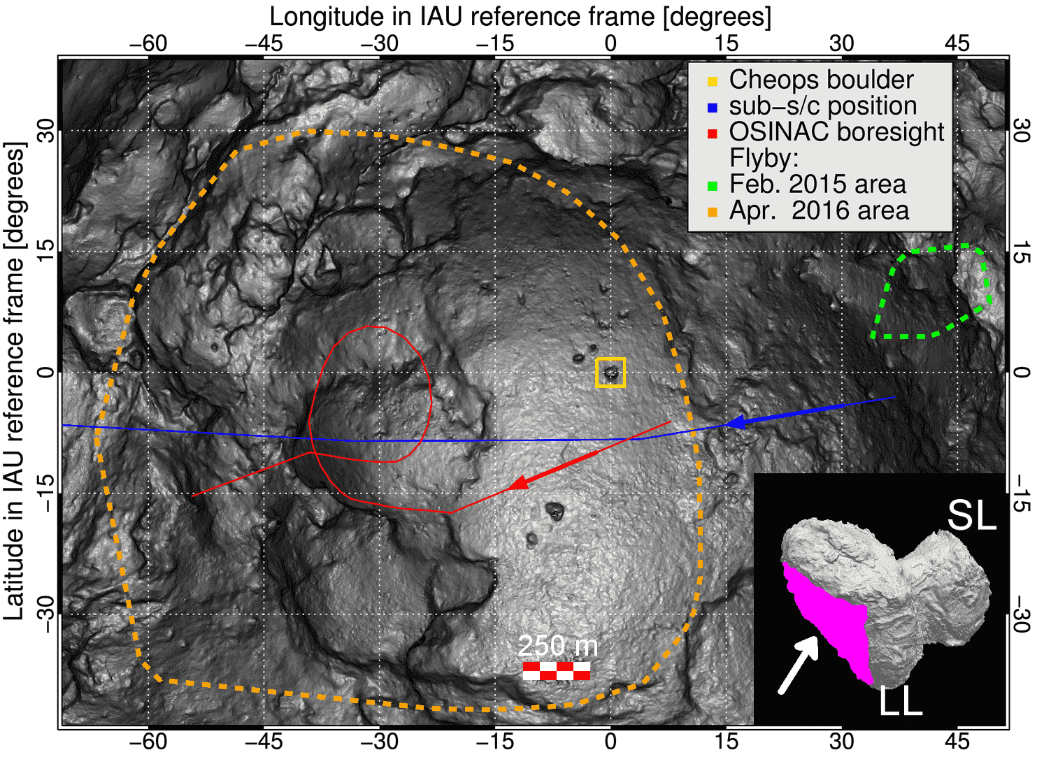
Figure 1: Context of 9-10 April 2016. Left (inset): Position of the Imhotep depression (in pink) with respect to the comet large lobe (LL) and small lobe (SL). (Main) Cylindrical projection centered on the Cheops boulder (gold square) of the Imhotep region, see main text for more details. Right: Curves of the median distance to the surface and median phase angle around the moment of closest approach during the flyby. The uncertainties correspond to the standard deviation of the values across each observation.

The left panel of Fig. 1 was produced using the “SPG SHAP7 v1.0” shape model with five millions facets and a horizontal spacing of about 2 meters (Preusker et al., 2017). In this figure, which we only produced for illustrative purposes, the brighter a facet, the smaller the angle between its normal and the direction from the nucleus center of mass to its barycenter. This means that the relative brightness of a facet in the left panel of fig. 1 is indicative of the local tilt. Additionally, the longitudes and latitudes are given here relative to the Cheops boulder (gold square) in order to properly accommodate the common area to the observations taken during the 14 February 2015 flyby (defined by the green dashed line), which lay just around the -180^∘/+180^∘ border in the Cheops reference frame (Preusker et al., 2015). In this frame, the coordinates of the Cheops boulder are +142.35^∘ E, -0.28^∘ S.
Additionally, in the left panel of fig. 1, the area common to all NAC observations taken during the flyby manoeuvre is delimited by the dashed orange line, while the sub-spacecraft position is marked by the continuous blue line. In this figure, the projection of the boresight of the OSIRIS NAC on the surface of the comet is indicated by the continuous red line.
Alongside the boresight of the OSIRIS/NAC, around the moment of closest approach, the median distance between the spacecraft and the nucleus surface varied between 28.6 and 29.2 km, as illustrated by the red dots in the right panel of Fig. 1. Hence, OSIRIS/NAC resolved the observed terrain with a resolution of about 0.53 m/px.

Observations. We list in Table 6 the OSIRIS/NAC observation sequences used in this study, as well their corresponding NAC filter image combination. We also list the median distance of the spacecraft to the surface elements, the corresponding spatial resolution for the NAC, the median phase angle, and the phase angle range as well as the position in longitude and latitude of the NAC boresight.
These observations were acquired around the moment of closest approach to the nucleus and either on an inbound or outbound trajectory from the moment of closest approach, which was reached during the first minutes after midnight on 10 April 2016.
For the analyses of this study, we chose to consider not only the observations acquired just around the moment of closest approach as a sequence of 3 NAC filter images (those centered at 480, 649, and 743 nm), but also two other sets of observations acquired shortly before and after the moment of closest approach using all of the 11 NAC filters (thus spanning the 269.3-989.3 nm wavelength domain), which also imaged the area in question under notably different illumination conditions (see the first and last lines in Table 6).
When these two additional sets of observations were included in our analysis, we found no evidence of morphological and structural differences that might indicate a major activity event in this area around the moment of closest approach.
As described in detail in Küppers et al. (2007) and Tubiana et al. (2015), when they were uploaded to Earth, these OSIRIS observations were reduced using the standard OSIRIS pipeline (the 1.0.0.34 version of the “OsiCalliope” software). In short, all these images were uncompressed, calibrated, radiometrically corrected, and converted from DN/s to radiance factor , and they were also corrected for geometric distortion.

Similarly to Fornasier et al. (2015); Feller et al. (2016) and Hasselmann et al. (2017), two further steps were added before the analyses: (1) we computed and retrieved the illumination conditions of the surface elements intercepted by each pixel of each image of the dataset, (2) we coregistered each image from each observation sequence to its corresponding F22 image, so as to force a correspondence between the pixels of each and every image of an observation sequence with the intercepted surface elements.
These two steps were achieved using software developed within the OSIRIS team. The first was assembled based partially on Gaskell et al. (2008) and Jorda et al. (2010). The latter step was written based on van der Walt et al. (2014) as a two-part process in which first, image features are detected with the “Oriented FAST and Rotated BRIEF” (ORB) algorithm (Rublee et al. (2011) or through an image segmentation and the use of an optical-flow algorithm (as based on Lucas and Kanade, 1981; Shi and Tomasi, 1994 and Bugeau and Pérez, 2009), and then, when the features were matched, each image was coregistered to the reference image using a homographic transformation.

In order to produce mappings of the illumination conditions, we used the “SPG SHAP7 v1.0” shape model of the nucleus, as detailed before. Furthermore, since at the time of these observations, the comet was only at 2.7 au, the Sun cannot be considered as a point-like source here. As noted in Shkuratov et al. (2011), the trigonometric relation expressing the angular diameter of Sun across the nucleus surface is arcsin(R_⊙/r), where R_⊙ is the radius of the Sun’s photosphere and r is the distance of the observed object from the Sun.
Hence, we can only sample phase angles greater than 0.095^∘. Therefore the phase angle ultimately ranges in our dataset from 0.095^∘ to 61.7^∘. In Table 6, phase angle ranges that have been truncated thus are denoted by a star.

3 Morphology of the flyby area

Throughout the ROSETTA mission, the nucleus of comet 67P has been shown to comprise a variety and a complexity of aspect and morphological structures, as discussed at length in Thomas et al. (2015a); El-Maarry et al. (2015); Auger et al. (2015); Massironi et al. (2015) and El-Maarry et al. (2016). The depression that is the Imhotep physiographical region is surrounded by the Apis, Ash, Bes, and Khepry regions.
As the spacecraft flew over this part of the comet (see the left panel of Fig. 1), OSIRIS/NAC acquired observations of the Imhotep depression and of the nearby regions Ash, Aten, Bes, and Khepry (see the right panel of fig. 2). Given the path of the spacecraft in these observations, we hereafter refer to the area of the April 2016 flyby as the Khepry-Imhotep transition.

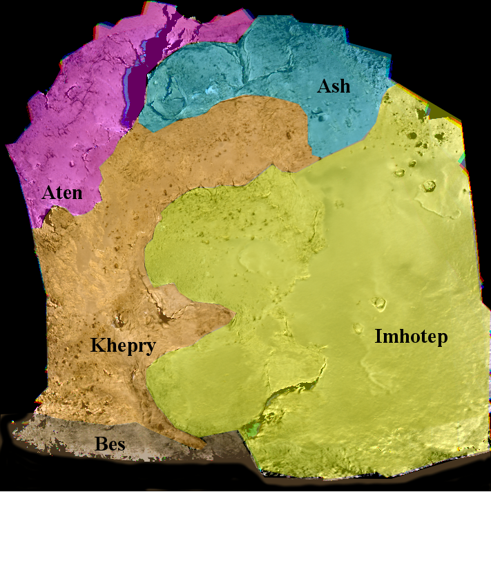
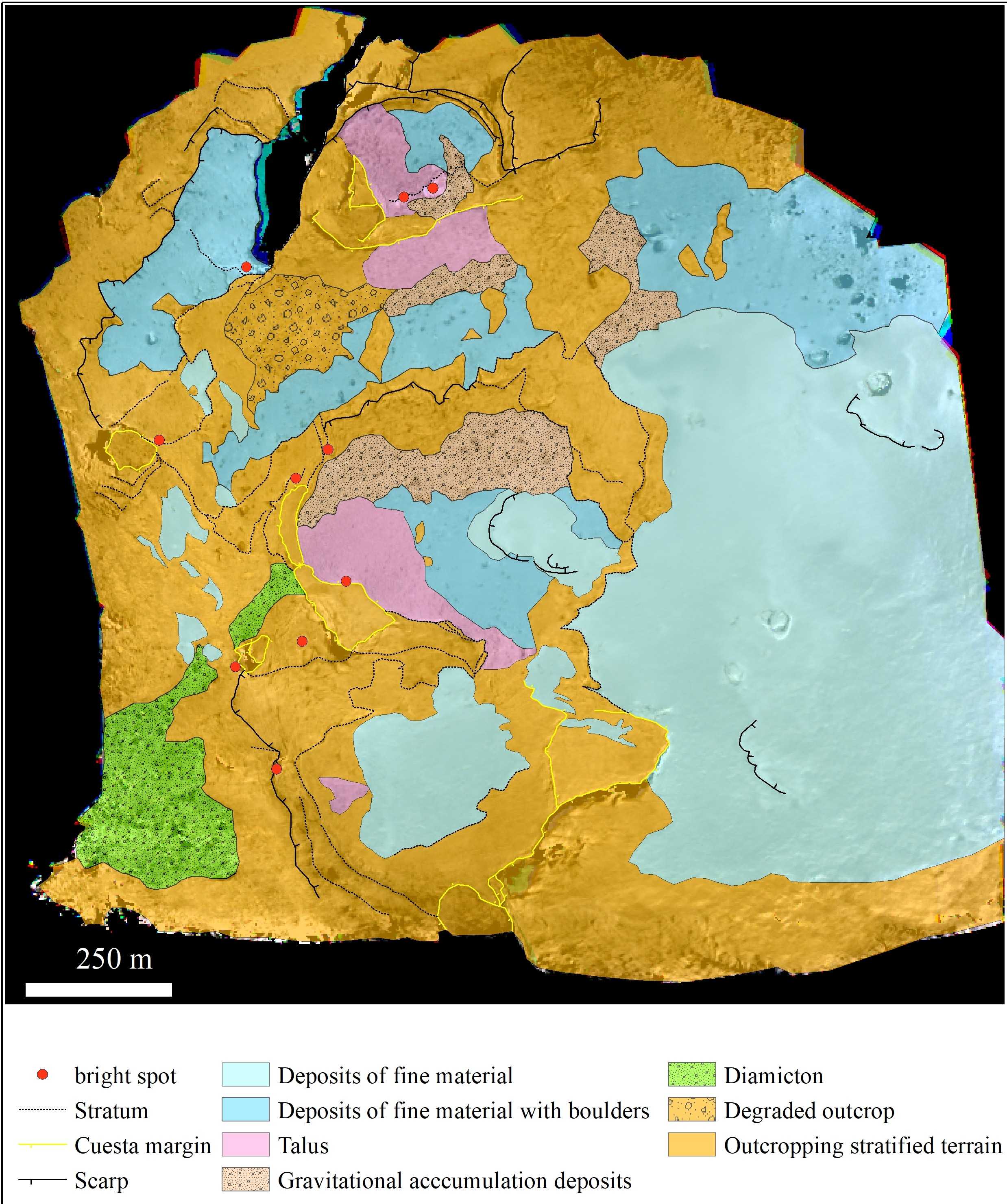
Figure 2: Left: RGB mapping of the flyby area overlaid with the limits of the corresponding morphological regions (see El-Maarry et al., 2015). Right: Geomorphological mapping of the transition area between Khepry and Imhotep. The peculiarities of the bright spots are discussed in the following sections.

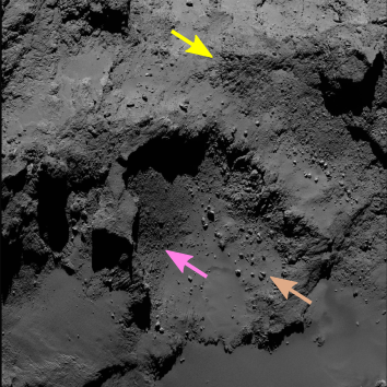
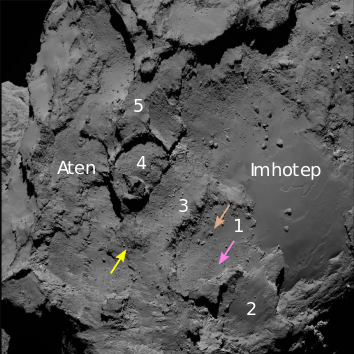
Figure 3: OSIRIS NAC observations of the Khepry-Imhotep transition region. Left (NAC 2016-06-09T08.47.10.761Z F22) arrows point toward degraded outcrops, talus, and gravitational deposits at the boundary between the Aten, Imhotep, and Khepry regions.
Right (NAC 2014-09-02T15.44.22.578Z F22): Between niches, consolidated materials form an ordered staircase structure, which from the deeper terrace labeled 1 rises up to the highest terrace labeled 5.

As detailed in El-Maarry et al. (2015) and El-Maarry et al. (2016), these regions all present different aspects and structure, but also common characteristics. While Ash, Aten, Bes, and Khepry present common features such as exposed consolidated material in the form of terraced and layered units and smooth deposits, Ash has been shown to be an area of airfall material deposit (Thomas et al., 2015b), and Bes hosts fractures and a pit.
Since the unconsolidated terrains of Imhotep are located in wide flat areas that correspond to the local gravitational lows, Auger et al. (2015) defined the region as a real accumulation basin for boulders and fine materials. In addition, along the side of the region that is being investigated and just before the perihelion passage, they observed that consolidated materials displayed bright patches despite their long-lasting exposure to illumination. This regeneration of bright patches on scarps has been associated with a progressive retreat driven by sublimation.

In the Khepry-Imhotep transition, as illustrated in the right panel of fig. 3, most of the surface terrains consist of consolidated materials that form terraces and niches because the Bes, Khepry, and Ash regions decline either toward the Imhotep or the Aten depressions (Giacomini et al., 2016) and (Lee et al., 2016). Imhotep in particular is indeed at a deeper structural level with respect to all these regions (Penasa et al., 2017), and on this specific side, is mostly filled by deposits of fine unconsolidated materials comprising low-density boulder fields or isolated megaclasts (Auger et al., 2015) and nucleating scarps. Outcropping layered terrains that surround depressions and niches form an ordered staircase structure of terraces (see the right panel of fig. 3).
The localized erosion of these terraces provides coarse surfaces (i.e., degraded outcrops, see the area indicated to by the yellow arrow in the right panel of fig. 3) or more evolved clast fields (i.e., diamictons) on their flat top, or clast deposits at the cliff base. The latter can be ascribed to a specific source and are distinguished in talus eposits, which consist of well-sorted clasts and gravitational deposits, which in constra imply well-graded unconsolidated materials supported by fine materials (see the left panel of fig. 3, the pink and brown arrows, respectively).
Terraces are partly covered by shallow deposits of fine material (i.e., unresolved regolith), which could likely be either the result of in-situ erosion or of airfall deposits, whereas their overhangs and steep ramps host most of the observed bright patches (bright spots in the right panel of fig. 2).

4 Global and local spectrophotometry

In the following section, we present the results of the spectrophotometric analysis of the region and of particular surface elements from the OSIRIS/NAC observations that were taken just around the moment of closest approach and were acquired using the filters centered at 480, 649, and 743 nm.

4.1 Global spectrophotometry

As shown in the right panel of fig. 1 and in Table 6, most of the NAC images of this dataset were acquired with a pixel scale of $\sim$0.53 m/px. In these observations, the phase angle densely samples the range between 0.1^∘ and 10^∘. Most of the shadows are therefore absent in these panels, and the contents of the niches, which are usually shadowed, are visible.
False-color images (hereafter RGBs), assembled from the NAC observations that wer acquired during the flyby area, are presented in the top panels of figs. 4 and 5. The spectral slope mappings (computed in the 535-743 nm range and normalized at 535 nm) corresponding to the RGB figures are shown in the bottom panels of figs. 4 and 6. As described in Fornasier et al. (2015), these spectral slopes were computed using the formula in Eq. 1,

$$S[\%/100nm]=\frac{R_{743nm}-R_{535nm}}{R_{535nm}}\cdot\frac{10^{4}}{(743.7[nm]-535.7[nm])}.$$ (1)

As in Feller et al. (2016), when absent, the radiance factor mappings at 535 nm were estimated in this study by interpolating between those observed at 480 nm and those at 649 nm. The resulting differences are discussed in section 4.4.
The spectral normalization was performed with the filter centered at 535 nm as no mineralogical bands are expected there, and in order to emulate the normalization using the V filter (Bessell, 1990) in the small-body literature.

In the RGB panorama (fig. 4) of Hasselmann et al. (2017), the transition area between the Khepry and Imhotep regions appeared to only slightly vary in terms of colors and spectral slopes, in the considered dataset and in the top panels in figs. 4 and 5 for instance, given the higher resolution and the lower range of phase angles, several additional structures and finer variations are evident.

Figure 4: Top: Panel of RGBs produced from 480nm, 639nm, and 743nm NAC filter images taken during the flyby. For clarity, the 2016-04-10T00h01 image has been rotated anticlockwise by 90^∘ . The positions of the bright surfaces discussed in the main text are denoted by red circles, while locations of groups of somber boulders are marked by green triangles. Bottom: Panel of the spectral slopes in the 535–743 nm range for the NAC images presented in fig. 8. The black circle in the right mapping encloses the surface elements for which the phase angle is lower than 0.095^∘. The symbols used in each image correspond to the surface elements investigated in fig. 8. See main text for details regarding the black and pink crosses and for the central cuesta structure encircled here in red. The red arrow points to the position of bright spot 44 in Deshapriya et al. (2018).

Figure 5: RGB from NAC filter images acquired at 23h46, before the moment of closest approach (see fig. 4). The red circles point to the location of bright surfaces, while the green triangles indicate groups of somber boulders. This figure encompasses all of the features investigated in this paper.

Figure 6: Spectral slope in the 535–743 nm range associated with fig. 5. The symbols used here and in the bottom panel of fig. 4 refer to the same surface elements. See fig. 8 for the corresponding measures. The red polygon defines the outcropping of spectrally blue consolidated material that is also marked in fig. 4 and is discussed in the main text.

The most striking features in this area are the bright blue-white patches located either in niches, underneath overhangs, or also among, at the tops of, or behind boulders. These features all present spectral slopes that are smaller than those of their surroundings. The position of the bright spots we investigated is marked by red circles in the top panels of figs. 4 and 5. A cursory investigation of the surfaces that are located close to overhangs and have a spectral slope smaller than 14 %/100 nm at these low phase angles (see fig. 6) points to circumferences that vary between 2 and at least 12 pixels (i.e., between $\sim$ 1 and 6 meters). The widest bright surface measured is located below the black upward triangle in the bottom right panel of fig. 4-b. Additionally, within the niche indicated by the pink square in the bottom left panel of fig. 4, the area of the whole bright surface is $\sim$ 160 m².

In the bottom right panels of figs. 4 and 6, another striking feature is the apparent unit of outcropping consolidated material with the inclined top (cuesta) that is delimited by the red polygon. The overall spectral behavior of this feature is smaller than its surroundings, which means that it might indicate an enrichment in water-ice rich material on the whole surface of the outcrop. The overall spectral slope of this unit is $\sim$ 17 %/100 nm at 4^∘ phase angle, while its surroundings are at $\sim$ 18 %/100 nm. This outcrop is the only such large unit of consolidated and stratified material in the flyby area that shows this behavior.
We furthermore observe that the surface of this terrain presents small variations of spectral slopes that closely follow the nature of the terrain: in contrast to terrains with a smooth aspect or those that lie at the top of the local cliffs, terrains presenting a rougher aspect or that have a higher declivity exhibit a slightly stronger spectral slope.

We also note that the spectral behavior of areas that are covered with fine material deposits (see the right panel of fig. 2) is smaller than that of their surroundings, but only slightly. For instance, in the bottom right panel of fig. 4, the material found at the top of the scarp (its location is indicated by the center of the pink cross) has a reflectance of 6.81$\pm$0.02% at 649 nm and a spectral slope of 17.9$\pm$0.1 %/100 nm, while the crown of the scarp directly next to it (its location is found just below the right arm of the pink cross, 13 pixels, about $\sim$6.9 m away from its center) has a corresponding reflectance of 6.54$\pm$0.02% and a spectral slope of 18.2$\pm$0.2 %/100 nm. This amounts to a mere 4.0% difference of the reflectance and only 1.7% disparity in spectral slope.
Similarly, between the red cross that marks the position of a fine material deposit (also referred to hereafter as UR-01), and the black cross just below it, which indicates the top of a consolidated material area whose surface is unresolved and apparently smooth, we find that the fine material deposit has a reflectance of 6.37$\pm$0.03% at 649nm (i.e., 3.8% lower than the consolidated material surface) for a spectral slope of 18.2$\pm$0.2 %/100 nm (i.e., 5.5% lower than the consolidated material).
These two examples illustrate the contrast and differences between these surface elements of the nucleus and that they can be perceived, even though they are weak.

Following this correlation between spectral behavior and terrain nature, we furthermore observe that in terrains that are covered with diamicton and areas where consolidated material emerges, talus and gravitational accumulation deposits are particularly distinguishable in the RGBs through their ochre-orange tinge, and in the spectral slopes mappings, they have values higher 18 %/100 nm.
A close inspection of the mappings further indicates that their variations are associated with a particular morphological feature. Most notably among the boulder fields, gravitational accumulation deposits, and outcrops of consolidated material, we also observe a widespread presence of large somber boulders and megaclasts among the different types of terrains in this area (see the right panel in fig. 2). The most obvious of the somber features is the 60 x 100 m² sized megaclast visible in the left panel of fig. 4 and in fig. 5.
Fig. 8 depicts the radiance factor in the orange filter images corresponding to the RGB presented in figure 4. We recall here that these images were photometrically corrected using the Lommel-Seeliger disk law (Seeliger, 1885 and Fairbairn, 2005). In the bottom right panels of figs. 4 and 8, the black circle at the bottom of the 2016-04-10T00h01 mappings delimits surface elements with phase angles smaller than 0.095^∘, as discussed in section 2.

Time (UTC)	23:34	23:46	00:01
Median phase angle (degrees)	4.0$\pm$1.3	3.0$\pm$1.0	1.2$\pm$0.6
Median I/F (at 649nm)	5.3$\pm$0.2%	5.8$\pm$0.2%	6.3$\pm$0.30%
Median S535-743nm (%/100nm)	18.0$\pm$0.6%	18.2$\pm$0.6%	18.3$\pm$0.6%
Brightest I/F value (at 649 nm)	20$\pm$3%	12.0$\pm$1.3%	14.0$\pm$1.7%
ID of measure	BF-01*	BF-08	BF-06
Symbol associated	red arrow	$\boldsymbol{\triangle}$	$\boldsymbol{\bigcirc}$
S535-743nm (%/100 nm)	8$\pm$11	4$\pm$1	5$\pm$3.7
Darkest I/F value (at 649 nm)	5.1$\pm$0.1%	5.5$\pm$0.1%	5.7$\pm$0.1%
ID of measure	SB-05	SB-05	SB-05
Symbol associated	-	$\diamond$	-
S535-743nm (%/100 nm)	19.5$\pm$0.3	19.7$\pm$0.2	19.5$\pm$0.3

Table 2: Details of the median and extreme radiance factor values in the measurements: the symbols are those used in Figs. 4, 8, and 8. The BF-01 measure is marked because this particularly bright surface has also been investigated as the ID-44 bright surface in Deshapriya et al. (2018); it survived for several months. The positions and the values of other particular measurements are reported in Table 7.

We assembled in Table 2 a summary of the median and some extreme values of the reflectance at 649 nm (as well as the corresponding spectral slopes). These latter values correspond to the extrema found among the surface elements we investigated, and they are further discussed in the next sub-section.
In fig. 8 a progressive overall decrease in contrast can be perceived as the spacecraft approached the moment of opposition, which indicates the observation of the opposition effect (e.g., Seeliger, 1885 and Shkuratov et al., 2011). Nevertheless, many features whose reflectances deviate by more than a sigma from the median I/F value are distinguishable from their surroundings.
This the case, for instance, for bright surfaces, which, as discussed previously, are found in niches, at the bottom of underhangs, or at the top of boulders. They are easily identifiable in fig. 8 as the white areas. Meanwhile, at the other end of reflectances, most of these easily identifiable surface elements are the somber boulders discussed previously that we indicate with green triangles in the top panel of figs. 4 and 5.

The values listed in table 2 show that the BF-01 measure is in particular distinguishable because it is close to four times the median reflectance of the observed area and has a standard deviation of 3%. This particular highest value measured for the radiance factor corresponds to one peculiar bright surface, referred to as BF-01 and as ID-44 in Deshapriya et al. (2018). It is located in a field of boulders and diamicton of the Khepry region, and its position is indicated by a red arrow in the upper left corner of figs. 4 and 8. This particular feature covers part of the boulder top. As it is extended well beyond the integration box, the measurement we report was performed around the brightest pixel (I/F $\sim$ 24%). We note that the DN/s values of the corresponding pixels are similar to but do not reach the saturation levels of the detector. This particular detail was also noted in most of the measurements performed over the course of several months that were reported in Deshapriya et al. (2016). This surface element is further discussed in the section on the 11-filter spectrophotometry.
Nevertheless, this feature is the brightest observed in the region of this flyby. For reference, in that same image, when we measure the radiance factor of BF-08 (the large bright patch close to an overhang, noted by a black triangle), we find a value of 12$\pm$1.3%/100 nm. As discussed below, the same bright spot was also observed on the next day at 11:50, and still had, at a phase angle of $\sim$64^∘, a radiance factor of 3.6$\pm$0.7%, while its surroundings appeared far darker, with a radiance factor of only about 1%.

Feature	UR-00	BF-02	BF-05	BF-06	BF-08	BF-010	SB-05
23h34	17.7$\pm$0.2	7.0$\pm$1.5	5.0$\pm$5.0	7.0$\pm$2.9	2.0$\pm$1.6		19.5$\pm$0.3
23h46	18.0$\pm$0.5		6.0$\pm$2.0	5.0$\pm$4.6	4.0$\pm$1.1		19.7$\pm$0.2
00h01	18.3$\pm$0.2		9.0$\pm$3.0	5.0$\pm$3.7		6.8$\pm$0.6	19.5$\pm$0.3

Table 3: Selection of spectral slope values in the 535–743 nm range: selection of values from the measurements marked in the right panel of figs.4, 8, and 8. The spectral slopes of the bright features (BF) are almost one-third of those of the smooth regolith (UR) and just less than one-fourth of those of the somber boulders (SB).

In a similar manner but at the opposite end of reflectances, the boulders exhibiting the red spectral behavior that we discussed above also distinguish themselves from their surroundings in these reflectances mappings through their lower-than-average reflectance. They present the same behavior independently of the phase angle at which they are observed.

4.2 Spectrophotometric analysis of local features

Figure 7: Panel of the photometrically corrected radiance factor images taken with the orange filter. From left to right: Image taken at 23h34, 23h46 and 00h01. The average phase angle is 4^∘, 3^∘ , and 1^∘, respectively. See fig. 4 for the symbol keys. The red square in the central figure points to the area observed in August 2016 that is shown in fig. 14.

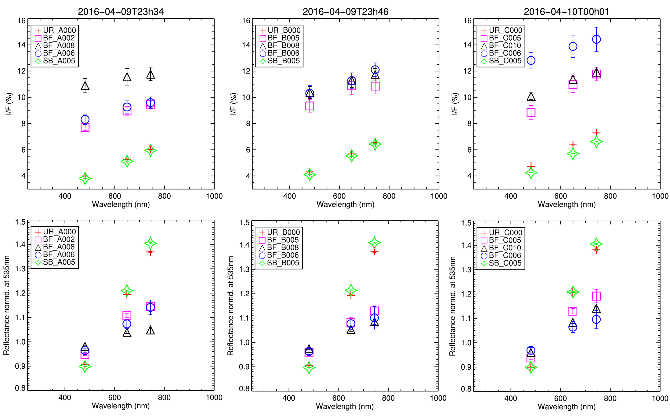
Figure 8: Panel of the result of the three-filter spectrophotometry measurements. Top: Reflectance (I/F) measurements. The bars indicate the dispersion of the values measured within the box and their propagation for the relative reflectance. Bottom: I/F measurements normalized at 535 nm. The key for the measurements IDs is, again, as follows: smooth, unresolved-looking, regolith (UR), bright feature (BF), and somber boulder (SB). The letter after the underscore indicates the 23:34 image (A), the 23:46 image (B), or the 00:01 image (C). Finally, the last three digits identify the feature among its particular type. See fig. 8 for an illustration of the measurement locations.

As this way, several dozens of surface elements were identified in the images as particular features of interest, for instance, bright patches, somber boulders, consolidated material, and unresolved regolith. From this collection of elements, we selected six features appearing in figs. 4, 8 and 8.
The radiance factor and spectral slope measurements were performed by integrating the signal in a 3x3 pixels box (i.e., 1.6 x 1.6 m²), unless otherwise noted. These measurements were made on both common and image-unique features. All images presented here have three measurements in common: a stretch of smooth regolith (red cross), a bright spot underneath a overhang (blue circle), and a somber boulder (green star). These measurements are identified by a tag: UR for very smooth unresolved-looking regolith, BF for bright feature, or SB for somber boulder (see fig. 8 and tables 2 and 3).
We show the results of the three-filter spectrophotometry in fig. 8.

Based on these measurements, we pursued the previously discussed notable distinction in behavior between the selected bright features and the other regions of interest. While somber boulders and smooth unresolved-looking regolith exhibit a similar behavior in both radiance factor and relative reflectance, all the selected bright features have a radiance factor at least twice that of the somber boulders or the unresolved regolith (see fig. 8 and table 7). Moreover, the bright surfaces also display smaller and less red spectral slopes than those of other surfaces and differ more widely from the slope of the average terrain. For the investigated terrains, for instance, while the spectral slopes of the somber boulders are between 1% and 19% higher than the slopes of the smooth regolith, the spectral slopes of the bright surfaces are between 10% and 87% smaller than those of the smooth-looking regolith. All corresponding values are assembled in table 3.

In the flybly area of February 2015 (encompassed by the green dashed line in the left panel of fig.1), some small bright surfaces were observed along the decline that leads toward the center of the Imhotep depression. However, these bright surfaces had reflectivities that would never be higher than 50% than the local average, and their spectral slopes were as high or greater than those of neighboring smooth terrains. These surfaces were interpreted to be partially richer in refractive materials and coated by deposits of organics (Feller et al., 2016).
Given the wider range of variations of the reflectance and the flatter spectra exhibited by the bright surfaces observed here, we interpret these surfaces to be of a similar nature to some of the surfaces investigated in Pommerol et al. (2015); Filacchione et al. (2016b); Barucci et al. (2016) and Oklay et al. (2016b), which were observed with the OSIRIS and VIRTIS instruments and were shown to be slightly richer in water-ice content, but only by a few percent. In this understanding, the more water-ice a surface element of the nucleus contains, the flatter its spectrum. A comprehensive study of such surfaces and of tentative modeling of their composition has been presented in Raponi et al. (2016).
Following the conclusions of these papers, we consider the surfaces to be appropriate candidates as locations enriched in water-ice material at the time of these observations. These locations should be further investigated and compared with possible VIRTIS observations.

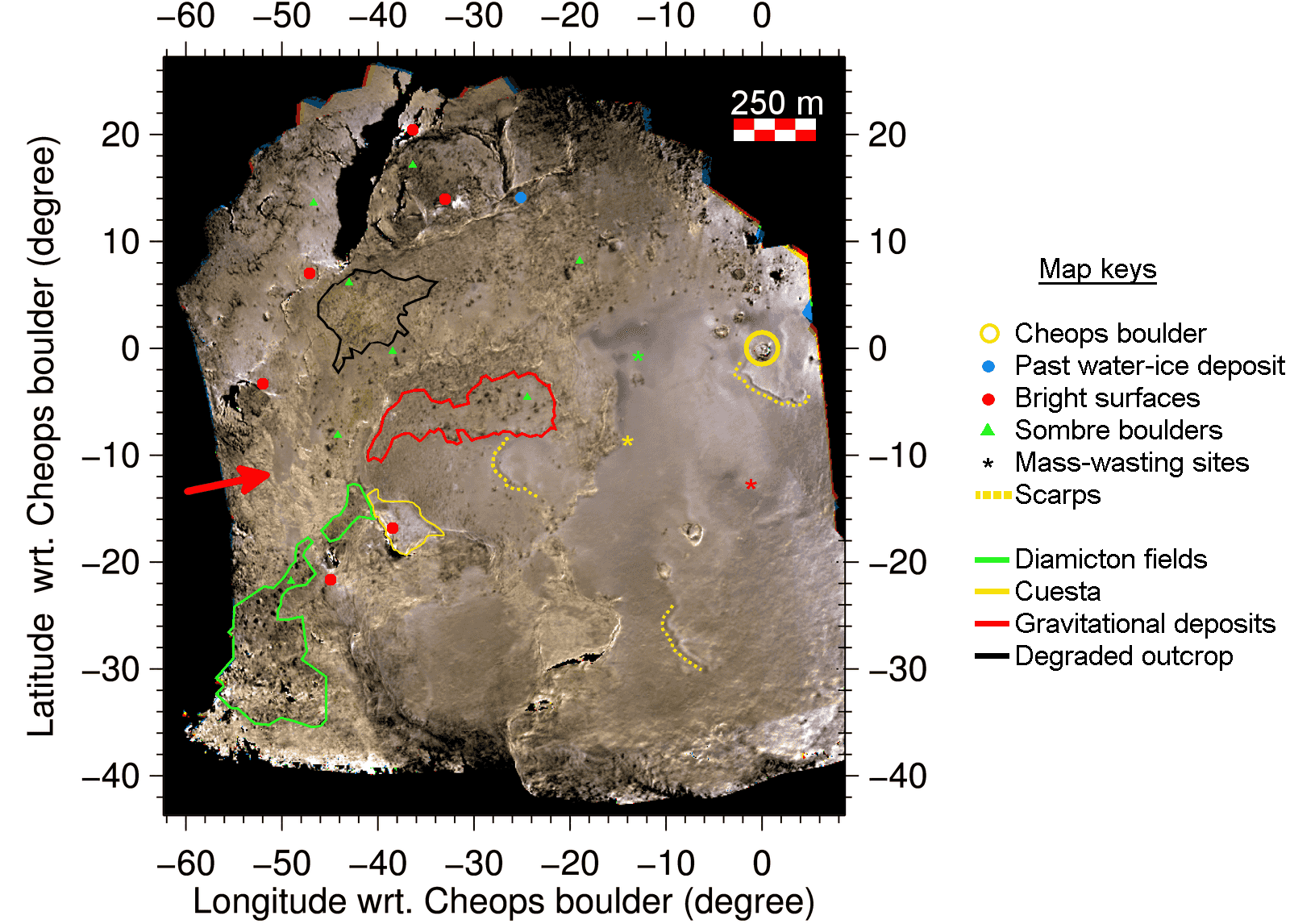
Figure 9: Georeferenced RGB of the April 2016 flyby region, assembled using photometrically corrected NF84, NF82, and NF88 images, and centered around the Cheops boulder. This mapping has a 0.1^∘x0.1^∘ resolution in longitude and latitude. The region shown correspond to areas visible in at least three of the considered observations. The locations where resurfacing processes were observed through the evidence of mass-wastings and moving scarps that were discussed in e.g. Groussin et al. (2015) and Deshapriya et al. (2018) are indicated. For clarity, only the largest bright spots are indicated, and the given positions of somber boulders point to their presence in all type of terrains, with the exception of the central depression of Imhotep.

4.3 Georeferenced RGB mapping

As the previously presented RGBs only allowed us to consider part of the flyby region as it was around the moment of closest approach, we have projected each photometrically corrected image onto a grid and assembled the results in a georeferenced RGB of the area (see fig. 9).
To produce this mapping, we have generated the georeference of each image to the SPG SHAP7 v1.0 model using ray-tracing and the reconstructed trajectory of the Rosetta spacecraft with respect to landmarks on the nucleus, computed during the generation of the SPC shape model.
We then projected the images onto a grid with a 0.1^∘x 0.1^∘ resolution in longitude and latitude, and averaged the reflectance by the number of times a grid element appeared in the observations. This resolution in longitude and latitude corresponds to a resolution of (2.7$\pm$0.3)x(2.7$\pm$0.3) m².

In this figure, the areas encircled by continuous lines correspond to some of the morphological units defined in fig. 2, the red circles and green triangles identify some of the bright surfaces and somber boulders, respectively. Scarps are noted here by the dotted yellow line, while a well-defined fine-dust deposit surrounded by consolidated material is indicated by the red arrow. Furthermore, the colored stars indicate areas pointed out by Groussin et al. (2015) as origins of resurfacing processes in the weeks before the comet passage at perihelion, while the blue circle indicates the position of pre-perihelion bright spots first discussed in Pommerol et al. (2015), where water-ice was detected (Filacchione et al., 2016a).
The variations in color and hue displayed in fig. 9 are a compelling indication of the multiplicity of terrain types. We recall that in a figure like this, a relative difference in brightness between two surface elements is indicative of a variation in geometric albedo, while a relative difference in color is indicative of a distinction of spectral behavior. We selected here and designated a few elements discussed previously, as well as in previous studies of this area.

While not all bright spots are apparent with this resolution, some of the bright surfaces (red circles in fig. 9 and in the previous figures) are still easily distinguishable. Those pointed here are the largest and located at the bottom of underhangs, except for two: one located around (-32^∘, +14^∘), found at a base of a niche of the Ash region, and another located close to (-46^∘, -22^∘) at the feet of a megaclast.
We note here that these two surface elements are both part of the source regions of two activity events that occurred around perihelion in August 2015. Both events are discussed in Fornasier et al. (ssue), and are numbers 42 and 133 in table A1.

Additionally, we also refer to Oklay et al. (2016a) for the investigation of the (-32^∘, +14^∘) bright feature (denoted there ROI7) in pre-perihelion images (NAC filter sequence acquired at 2014-09-25 06:46:25 UTC). This bright feature was then notably compared to the area marked by a blue circle (-26^∘, +14^∘), which was also found to harbor particularly bright boulders and surface elements whose spectral slope was lower than their surroundings (Pommerol et al., 2015 and Oklay et al., 2016a). This particular area, observed by the VIRTIS instrument in October 2014 and labeled BAP-1 in Filacchione et al. (2016a), was found to have spectral properties that are best fit with a water-ice content that varies between 1.2% and 3.5%, depending on the mixing scenario the authors considered (areal or intimate mixing), and are therefore one of the very first nucleus regions where emerging water-ice-rich material was ascertained.

The two bright surfaces, located around (-44^∘, +8^∘) and (-38^∘, +20^∘), are both particularly evident in the spectral slope mappings of the bottom left panel in fig. 4, and BF-010 and BF-011 have geometric albedos at 649 nm of 11.3% and 8.9%, respectively (i.e., $\sim$ 66% and 31%, respectively, higher than the nucleus average of 6.8%) and spectral slopes of 6.8% and 9.0% (i.e., $\sim$ 62% and $\sim$51%, respectively, lower than the region average of 17.98 %/100 nm at $\alpha$ = 0^∘, see fig. 13). These two surfaces are found at the bottom of large declivities, and the nature of the topography between the morphological regions Ash and Aten is only well rendered in fig. 9 by the actual absence (areas in black) of observations of these cliffs during the flyby manoeuvre.

For similar reasons, the bright surface located around -55^∘of longitude and -2^∘of latitude, identified in this study as BF-08, also stands out because during the 23h34 and 23h46 observations, its reflectance was at higher than 11%, while its spectral slope ranged between 0.8 and 5.1%/10 nm (i.e., between $\sim$72% and $\sim$96% lower than the region average).
Following the previous remarks, it is therefore most likely that these bright surfaces harbor water-ice-rich material.

Similarly, in this mapping, the largest somber boulders are also still distinguishable in different parts of the region (see the green triangles in fig. 9). They are found to be on most types of morphological units: diamictons (green polygons), fine-material deposits covered with boulder fields, fine-material deposits (e.g., the lone boulder in Aten in between the two bright surfaces), as well as among the gravitational accumulation deposits (red polygon) and the degraded outcrops (black polygon). We note, however, that they are absent from the fine-material deposits that cover the smooth central region of the Imhotep depression, as well as from two of the taluses of the area.
We note here that such boulders with a lower-than-average reflectance and a red spectral behavior have also been observed in the area of the February 2015 flyby (Feller et al., 2016).

Other areas of this flyby region present a contrast as clear as that of somber boulders and their neighboring terrains, for instance, the area indicated by the red arrow in fig. 9, where previous fine-material deposits cover the top of a series of terraces whose fronts are formed by the outcropping consolidated material. Moreover, scarps within fine-material deposits are clearly visible. They are denoted by the yellow arrows in the corresponding figure. Such features were evident in pre-perihelion images, for instance, the red star marks the linear feature shown in Thomas et al. (2015b). During the approach to perihelion, however, some new scarps appeared or progressed across the surface, exposing resurfacing processes of the smooth central area of Imhotep (Groussin et al., 2015), with evidence of mass-wasting processes around the location marked by the yellow, green, and red stars as well. These resurfacing processes are also discussed in Deshapriya et al. (2018). We also note here that the area around the red star was the source from another activity event observed in NAC observations acquired on 12 August 2015 (see entry 151 in table A1 of Fornasier et al., ssue).
While the contrast between the top and bottom of these scarps is well marked in this figure and the outline of the scarp close to (-20^∘, -10^∘) is even evident at a low phase angle (see the right panel of fig. 8), the differences in the corresponding spectral slope mapping are notably small (see fig. 6) as it presents itself as a variation of less than 2 %/100 nm around the local average spectral slope value.

The flyby area is distinguished by the diversity of morphological units, as well as by the variety of colors of these different terrains and of particular features such as bright spots and somber boulders. Furthermore, this particular region of the comet can be deemed of a particular interest as it encompasses numerous surfaces elements where cometary activity and surface evolution have been observed as the comet approached, passed through perihelion, and moved away from it. The source locations of jets and outbursts observed around perihelion are shown in fig. 1 of Fornasier et al., submitted. For instance, the area where niches hosts two large bright surfaces located around (-32^∘, 14^∘) was observed on 1 August 2015 to be the source of one particular large outburst. Such bright surfaces were not evident in OSIRIS/NAC images acquired in September 2014 (Auger et al., 2015 and Oklay et al., 2016b), but further indicate compositional heterogeneities on the nucleus immediately below the dust mantle, that are revealed as the insolation is sufficient to pierce through this insulating layer and trigger a violent activity event, such as has been observed for cliff collapse (Pajola et al., 2016 and Fornasier et al., 2016).

4.4 NUV, Vis, and NIR spectrophotometry

We present here the results acquired from the two sequences of observations taken before and after the moment of closest approach using the 11 NAC filters between 269 and 989 nm.
These two sequences were found to be best coregistered when segmentation and optical flow algorithms were combined. Considering the difficulty of correcting the parallax effect for the full image, we chose to integrate the signal in 5x5 pixels boxes, which corresponds to a surface element of 24.5 m². We used both sequences to investigate some particular surface features as well as to constrain the differences of spectral slopes described previously.

We present in fig. 10 the reflectance mappings and mappings of the spectral slope computed in the 535-882 nm range for the 2016-04-10T11h50 observation sequence. As in previous observations, we note the same apparent anticorrelation between the brightness (in radiance factor) of an area, its morphological type, and the steepness of its spectral slope.
In these figures, areas that were previously identified as fine-material deposits (such as terraces and surfaces close to the bottom of underhangs) appear slightly brighter and present a smaller spectral slope. Similarly, the consolidated material structure encircled in red in the bottom panel of fig. 4, although it has a reflectance that is almost average, still exhibits, at $\sim$ 51^∘of phase angle, a spectral slope slightly lower than 17 %/100 nm. This observation supports the previously stated conclusion that this feature likely is a large-scale (of about 100 m) compositional heterogeneity.
Meanwhile, the structures that are identified as eroded consolidated material, diamictons, or boulder fields here also present a reflectance that is slightly lower than average and a higher spectral slope.
In these figures, one feature that is not visible in other NAC images is the large bright surface close to the underhang with a low spectral slope. This area is also distinguished through its particularly smooth appearance. This feature was one of the bright spots whose photometric properties were investigated in Hasselmann et al. (2017) and were found to best match the remnants of a sublimated intimate mixture of water-ice, carbon black, and tholins studied in Jost et al. (2017a). We further investigate its spectrophotometric properties below.

In this sequence, we investigated the bright spot on the boulder that were previously identified (BF-01, blue circle), a neighboring unresolved-appearing terrain (orange square, UR-02), a bright smooth surface underneath an overhang (green star, BS-01), the previously investigated smooth-looking regolith (red cross, UR-00), a smooth area in a degraded outcrop of consolidated material (black upward triangle), and a somber feature in fine-material deposits on Imhotep (magenta downward triangle, SF-01). We report the results of the spectrophotometric analysis in fig. 11.

Figure 10: 2016-04-10T11h48 sequence ($\alpha$ $\sim$ 51^∘): Maps of the photometrically corrected radiance factor (left) and of the spectral slope in the 535–882 nm range (right). The symbols refer to the measurements made and presented in fig. 11. Under these illumination conditions ($\alpha$ $\sim$ 51^∘), the shadows are cast on the niches and areas where bright material was previously observed (see fig. 4).

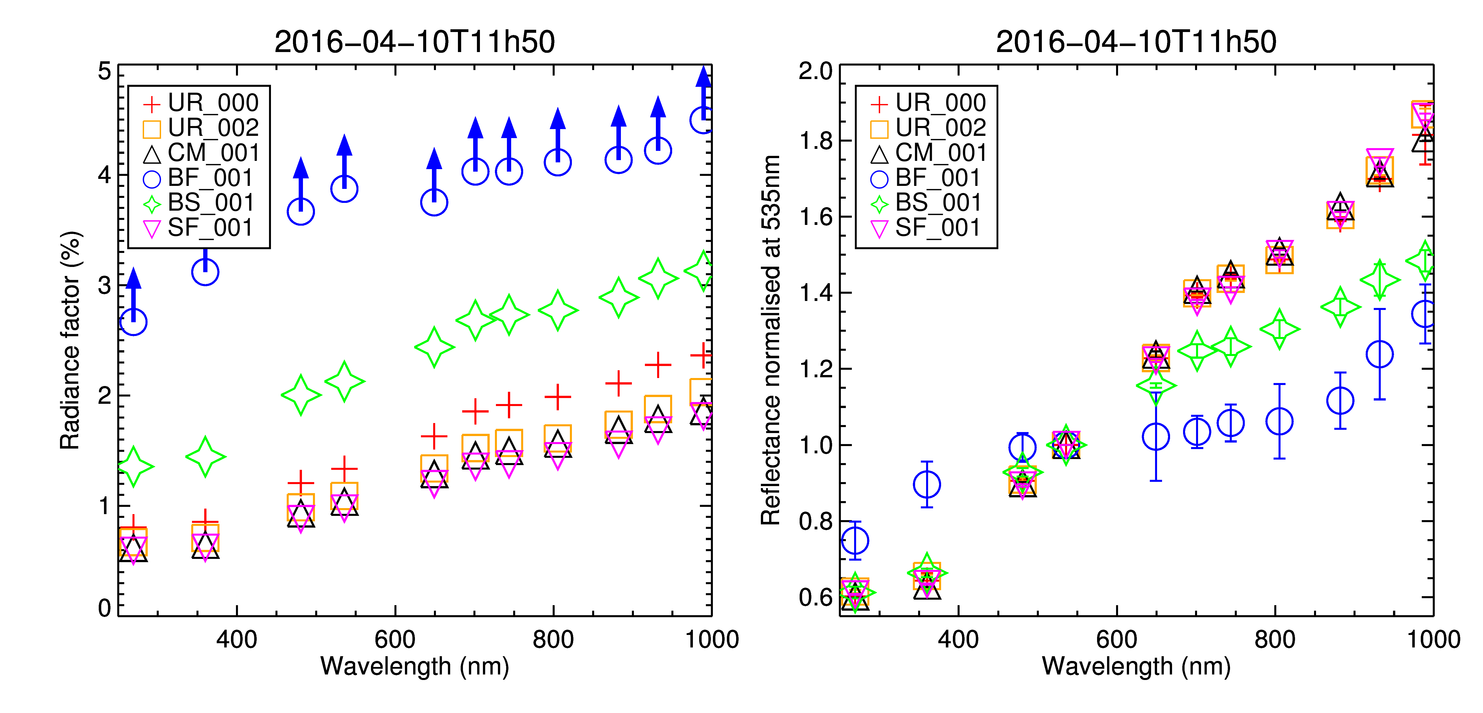
Figure 11: Spectrophotometry measurements for the 2016-04-10T11h48 sequence. The images were photometrically corrected using the Lommel-Seeliger disk law. The symbols correspond to the measurements made at the locations indicated in fig. 10a. We note here that the measures for BF-01 were close to the detector saturation levels. These values therefore correspond to lower limits.

We report here the values of the spectral slopes in the 535–743 nm range for the measurements that were made without correcting for the phase-reddening phenomenon (see following section). These measurements are (in %/100 nm) 20.4$\pm$0.4 for UR-00, 20.0$\pm$0.9 for UR-02, 20.9$\pm$0.4 for CM-01, 3$\pm$6 for BF-01, 12$\pm$2 for BS-01, and 19.2$\pm$0.7 for SF-01.

Figure 11 shows that the smooth-looking terrain and the consolidated material exhibit a similar red spectral behavior, as has been observed previously in the high-resolution images of the February 2015 flyby. This spectrum for the average smooth-looking regolith terrain (UR-00) is typical of the average dark terrain of the comet nucleus (see, e.g., fig. 2 in Fornasier et al., 2016). However, contrary to what was observed in February 2015, the bright surfaces of this area (BF-01 or BS-01) have spectra sensibly different from smooth surfaces or consolidated material. Moreover, the selected bright areas are at least twice as bright (in terms of radiance factor) as the average smooth-looking regolith terrain.
We indicate here that in all of these observations, the reflectances of the bright feature at the top of a boulder (called BF-01 in this study and ID-44 in Deshapriya et al. (2018)) were again similar to but did not reach the saturation levels of the NAC. This is denoted by the blue arrows in the left panel of fig. 11.
We observe, as noted previously with the three-filters observations, that the smooth unresolved-looking regoliths, the surfaces among the eroded outcrop, and the somber feature exhibit similar characteristics: the reflectance is considerably lower than those of the bright features, and they share a very similar spectral behavior. On the other hand, the two identified bright features have very low spectral slopes at $\sim$51^∘ phase angle and noticeably fainter normalized reflectances. We interpret these surfaces to be fractionally enriched in water-ice material (Filacchione et al., 2016b; Barucci et al., 2016; Deshapriya et al., 2016; Fornasier et al., 2016 and Oklay et al., 2016b) , and the observed differences between these two surfaces might reflect a further difference in composition, as considered in Deshapriya et al. (2018).

We also considered these two sequences with 11 filters in order to constrain the differences in spectral slopes using different computing methods.
In previous studies, spectral slopes have been computed in the 535-882nm range when the corresponding OSIRIS images were available. Spectral slopes have otherwise been computed in the 535-743 nm range, using either the F23 filter image, or an interpolation using the F24 and F22 filter images. We present in fig. 12 the corresponding mapings.

We have investigated the global variations of the spectral mappings assembled from the 2016-04-09T12h13 and 2016-04-10T11h50 observations, as well as some local variations between the assembled 2016-04-09T12h13 spectral slope mappings.
For each observation, we applied a Gaussian fit to the different spectral slope mappings to determine the center of the distribution and its full width at half-maximum (FWHM). The results are assembled in table 4.

Observation	$\Delta\lambda$ (nm)	S (%/100 nm)
9th/04 - 12h13	535 - 882	17.8$\pm$2.2
$\alpha$ $\sim$ 62∘	535 - 743	21.6$\pm$2.9
	535* - 743	21.2$\pm$2.6
10th/04 - 11h50	535 - 882	17.6$\pm$2.3
$\alpha$ $\sim$ 51∘	535 - 743	21.0$\pm$3.0
	535* - 743	20.4$\pm$2.6

Table 4: Differences in spectral slopes: spectral slope values (S, center, and FWHM) of the Gaussian fitting for each spectral slope mapping considering their wavelength range ($\Delta\lambda$). The asterisk denotes that the corresponding 535 mappings were interpolated from the associated 480 nm and 649 nm filter images.

We note that based on these results for the 12h13 observations, the spectral mapping in the 535-882 nm range is $\sim$21% and $\sim$19% lower than the 535-743 nm and the 535* -743 nm spectral mappings. Similarly, for the 11h50 observations, the spectral slopes mapping in 535-882 nm range is $\sim$19.5% and $\sim$16.5% lower than the other two spectral mappings.

Location	Spectral slope range (nm)
	535 - 882	535 - 743	535* - 743
ROI - A	17.7 $\pm$ 0.7	21.2 $\pm$ 0.5	20.8 $\pm$ 0.5
ROI - B	17.2 $\pm$ 0.2	20.3 $\pm$ 0.4	20.0 $\pm$ 0.4
ROI - C	18.5 $\pm$ 0.5	22.3 $\pm$ 0.5	21.6 $\pm$ 0.7
ROI - D	18.1 $\pm$ 0.2	21.6 $\pm$ 0.2	21.7 $\pm$ 0.3
ROI - E	14.7 $\pm$ 0.2	19.5 $\pm$ 0.7	20.8 $\pm$ 0.5
ROI - F	15.2 $\pm$ 0.3	19.1 $\pm$ 0.4	18.9 $\pm$ 0.4

Table 5: Comparison of the spectral slope ranges: Different spectral slope values for the different regions of interests indicated in fig. 12.

We further list in Table 5 local measurements of the spectral slopes around the Imhotep region, including areas outside the Imhotep-Khepry transition. Following the previous remark, we find once again that the 535-882 nm spectral slope measurements are on average 20$\pm$5% lower than the 535-743 nm spectral slopes, or 18$\pm$9% lower than those computed between 535nm (interpolated) and 743nm.
In both cases, the extreme values come from the measurements of the strikingly blue regions (i.e., those with a lower slope than average) in fig. 12. These 535-882nm measurements differ by 32% and 26% from the corresponding 535-743nm values and by 41% and 24% from the corresponding 535*-743nm values.
These areas are part of a region of the nucleus where water-ice-rich material and outbursts have been observed (Knollenberg et al., 2016; Deshapriya et al., 2018; Oklay et al., 2016b and Agarwal et al., 2017. They also encompass the feature described as “blues veins” in Hasselmann et al. (2017), whose photometric properties were best matched by those of the remnants of an intimate mixture of water-ice, carbon black, and tholins after sublimation. The noted spectral difference is therefore very likely to derive from a compositional difference. As there appears to be an overall shift down of the 535-882 nm spectral slopes in the bottom left corner of the mapping with respect to the others, however, we note here that this local difference in values might be due to a new flat-field correction for the NAC F24 filter (centered at 535nm) that was implemented in-flight in late 2015. While this artifact might slightly overestimate the noted particularity of this area (by $\sim$9% compared to the other two measurements), we still correctly observe that this area is different from the other neighboring areas (see the other mappings in fig. 12).

Figure 12: From bottom to top: Spectral slopes computed in the 535-882 nm range, in the 535-743 nm range, or in the 535-743 nm range with an interpolation at 535 nm. Each spectral slope mapping has its own color bar, adjusted within $\pm$7$\sigma$ around the median value.

4.5 Phase reddening

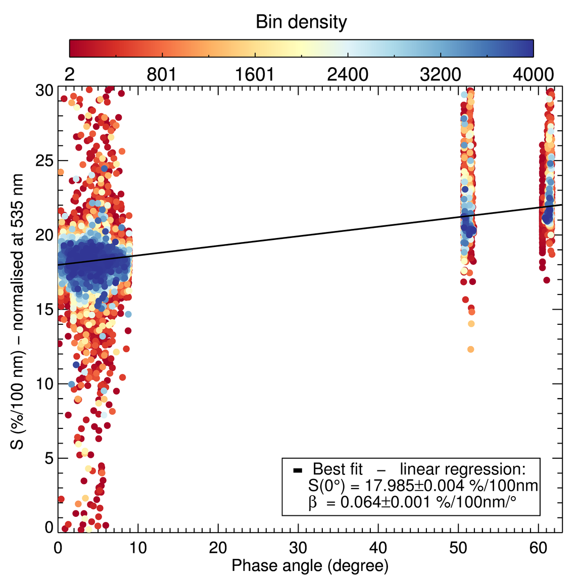
Figure 13: Phase reddening observed above the Khepry-Imhotep region during the flyby. Using the density of each bin as weights, the linear best-fit solution gives a spectral slope at 0^∘ and a phase reddening slope similar to that measured in Feller et al. (2016).

Phase reddening is the increase in spectral slope with the phase angle, first observed on the lunar surface (Gehrels et al., 1964). As discussed at length in Jost et al. (2017a), this phenonemon has also been observed in laboratory settings (Gradie et al., 1980) as well as on asteroids (Clark et al., 2002 and Sanchez et al., 2012). The ROSETTA mission parameters have allowed us soon after rendezvous with the comet to provide the first definite phase-reddening measurement on a comet Fornasier et al. (2015). As in our previous studies (Fornasier et al., 2016 Feller et al., 2016), we have sought here to constrain the measure of the phase reddening in the Imhotep-Khepry transition as the comet was at 2.7 au away from the Sun.
To this effect, we computed the spectral slope mappings for each sequence of images listed in table 6 and then ran a linear regression.

The density plot of the spectral slopes computed for this dataset and their linear best-fit solution are shown in fig. 13.
Around the morphological transition between Khepry and Imhotep, in the 535-743 nm range, and between 0.1^∘ and 62^∘ of phase angle, these spectral slopes are best fit by a slope of 0.064$\pm$0.001 %/100 nm/^∘ and a spectral slope at $\alpha$=0^∘ of 17.985$\pm$0.004 %/100 nm.

We note that these results are quite similar to those obtained for the part of the Ash-Imhotep transition flyby in February 2015, which were 0.065$\pm$0.001 %/100 nm/^∘ and 17.9$\pm$0.1 %/100 nm, as the comet was 2.3 au inbound to perihelion. We recall that the flyby discussed here took place while the nucleus was 2.7 au outbound.
While the values of these 535-743 nm spectral slopes are $\sim$ 17$\pm$5 % higher than their 535-882 nm counterparts, the phase-reddening slopes are nevertheless consistent with those measured in the 535-882 nm range over one rotational period of the nucleus, between August 2014 and February 2016, as listed in Fornasier et al. (2016).
As shown in that study, the phase-reddening slope of the nucleus abated from 0.104 to 0.041 %/100 nm/^∘between August 2014 and August 2015 (inbound to perihelion), before a further increase between August 2015 and February 2016 (outbound from perihelion) at least up to the initial phase-reddening slope of 0.104%/100 nm/^∘. Thermal modeling by Keller et al. (2015) and analysis of detailed nucleus observations by El-Maarry et al. (2016) have lead to the interpretation of this variation as a likely consequence of the global thinning of the dust mantle across the nucleus that is observed around perihelion (on an order of magnitude of 1 m during this passage), and the change in surface properties, such as dust roughness and the composition of the uppermost layer.

This area, which has been the source region of several jets during that passage of the comet through the inner solar system, is also the area where most of the fine-material deposits of the Imhotep central area went through a resurfacing process in the weeks before perihelion. Likewise, this is the area where evidence of diurnal and seasonal water cycles were observed (Fornasier et al., 2016), and where more surfaces likely containing water-ice material are exposed on the surface by April 2016 than in August or September 2014. These surfaces were then, at 2.7 au, likely to survive until the approach to the next perihelion passage.
We therefore interpret the increase in phase-reddening slope outbound from perihelion to reflect the complex nature of the changes that occurred and were occurring on this part of the nucleus surface and the transition in terms of cometary activity as its heliocentric distance grew.

5 Discussion

The OSIRIS/NAC observations taken during the April 2016 low-altitude low-phase angle flyby show in great detail the complexity of the transition between the morphological regions Imhotep and Khepry. While this area is similar to most of the overall nucleus surface, it contains a variety of morphological features as well as a diversity of behaviors in terms of colors and spectral properties.
Moreover, it shows some striking differences with the part of the transition area between the Ash and Imhotep regions that the spacecraft crossed during the February 2015 flyby (Feller et al., 2016) and that was surveyed with a 12 cm/px resolution.

In the Ash-Imhotep transition area of the February 2015 flyby (see also table 8), the part belonging to the Ash morphological unit appeared to be coated with fine-material deposits and peppered with decimeter- and meter-sized boulders, while the 400 m slope, leading toward the center of the Imhotep depression, consisted of strata of consolidated material covered with sparse boulders and a few small localized surfaces where fine material and pebbles are visible.
On the other hand, the Imhotep-Khepry transition presents a terraced topography where several extended fine-material deposits are visible on Imhotep, Khepry, and part of Aten. It also hosts large features of consolidated material, as well as areas of degraded outcrops, diamicton, taluses, gravitational accumulation deposits, and boulder fields.

These two transitions further differ from one another in their global spectrophotometric properties. Some degree of difference was already indicated by August 2014 observations where at $\sim$ 1.3^∘of phase angle, the Ash-Imhotep transition exhibited reflectances at 649nm lower than 5.1%, and a 553-882 nm spectral slope higher than 13.5 %/100 nm, whereas the Imhotep-Khepry transition presented reflectances of about 5% and higher, and corresponding spectral slopes between 11 and 14 %/100 nm (see fig. 9 in Fornasier et al., 2015). Similarly, in fig. 13 of Fornasier et al. (2015), at around 10^∘  phase angle, the former transition only displayed strongly elevated spectral slope values, while the latter presented a range of moderate and elevated spectral slopes values. Based on these observations, the Ash-Imhotep transition could then be classified as belonging to a group of terrains with high spectral slopes, and the Imhotep-Khepry to the group of terrains with intermediate spectral slopes.

This group of terrains also included the regions close to the top of the small lobe of the comet, such as Agilkia. This particular region, investigated in La Forgia et al. (2015), shows clear variations in the assembled normal albedo and spectral slope mappings. As indicated by the authors, the comparison of these mappings with the corresponding morphological map points to a correspondence between the reflectance, spectral slope, and morphological nature of a terrain. In particular, it was observed that around the Agilkia area, the fine-material deposits exhibited on average a slightly higher reflectance and a lower spectral slope (computed following Jewitt and Meech (1986) in the 480-882nm range) than their locally surrounding diamicton fields, taluses, gravitational accumulation deposits, or neighboring outcropping layered terrains.
As apparent in the mappings of the previous section, a similar observation can be made for the Imhotep-Khepry transition. While in the reflectance mappings uneven and rough surfaces (e.g outcropping stratified terrains or degraded outcroppings) appear only slightly darker in this area than fine-material deposits, a clearer contrast arises from the spectral slope mappings in which smooth areas of fine-material deposits stand out from their rougher surroundings (e.g., diamictons or taluses). Other outstanding features add themselves to this general picture, such as the somber boulders, bright surfaces in niches, or close to underhangs and the large consolidated material feature encircled in red in the bottom panel of fig. 4, which presents lower-than-average spectral slopes at its head and flanks.

While investigations into the nature of somber boulders are still ongoing, the bright surfaces displaying low spectral slopes that are essentially found in niches or at the bottom of underhangs, exhibit a behavior that is typically associated with areas that are enriched in water-ice material, as explained previously.
Any enrichment in water-ice material would be only fractional, however, as discussed in previous studies (Sunshine et al., 2006; Filacchione et al., 2016b; Barucci et al., 2016; Oklay et al., 2016b and Fornasier et al., 2016). In particular, the analysis of surfaces observed by the VIRTIS infrared spectrometer, in which bright surfaces were visible, led by Raponi et al. (2016), has indicated that areas presenting a spectral slope lower than 10 %/100 nm in the 500-1000 nm range at a phase angle of 95^∘  could be composed of just over 1% of pure water-ice in an areal mixing scenario and of well over 5% in an intimate mixture scenario.
Additionaly, the area denoted by a blue circle in fig. 9, where bright surfaces have been identified by Pommerol et al. (2015), was considered to host material enriched by up to 6% in water-ice according to infrared spectrum modeling (Filacchione et al., 2016b). For some of the surface elements of the same area, Oklay et al. (2017) have obtained corresponding values ranging from 6% to 25% based on the spectrophotometric properties of these spectral regions and thermal modeling. Similarly, the analyses conducted in the Anhur and Bes on some of the singular very large compositional heterogeneities have indicated local $\sim$ 20% and $\sim$ 30% enrichment in water ice (Fornasier et al., 2016 and Fornasier et al., 2017).

At this time, we cannot report any constraint on the water-ice enrichment of the observed bright surfaces from the considered dataset. We can report, however, that some of the bright surfaces have been observed several times during the mission and that investigations of a temporal variation in their spectrophotometric properties is currently being undertaken. For instance, we have found the bright feature BF-06 and another bright feature close to UR-0 to clearly present once again in August 2016 at 3.5 au a spectral behavior that is consistent with a water-ice material enrichment (see fig. 14).

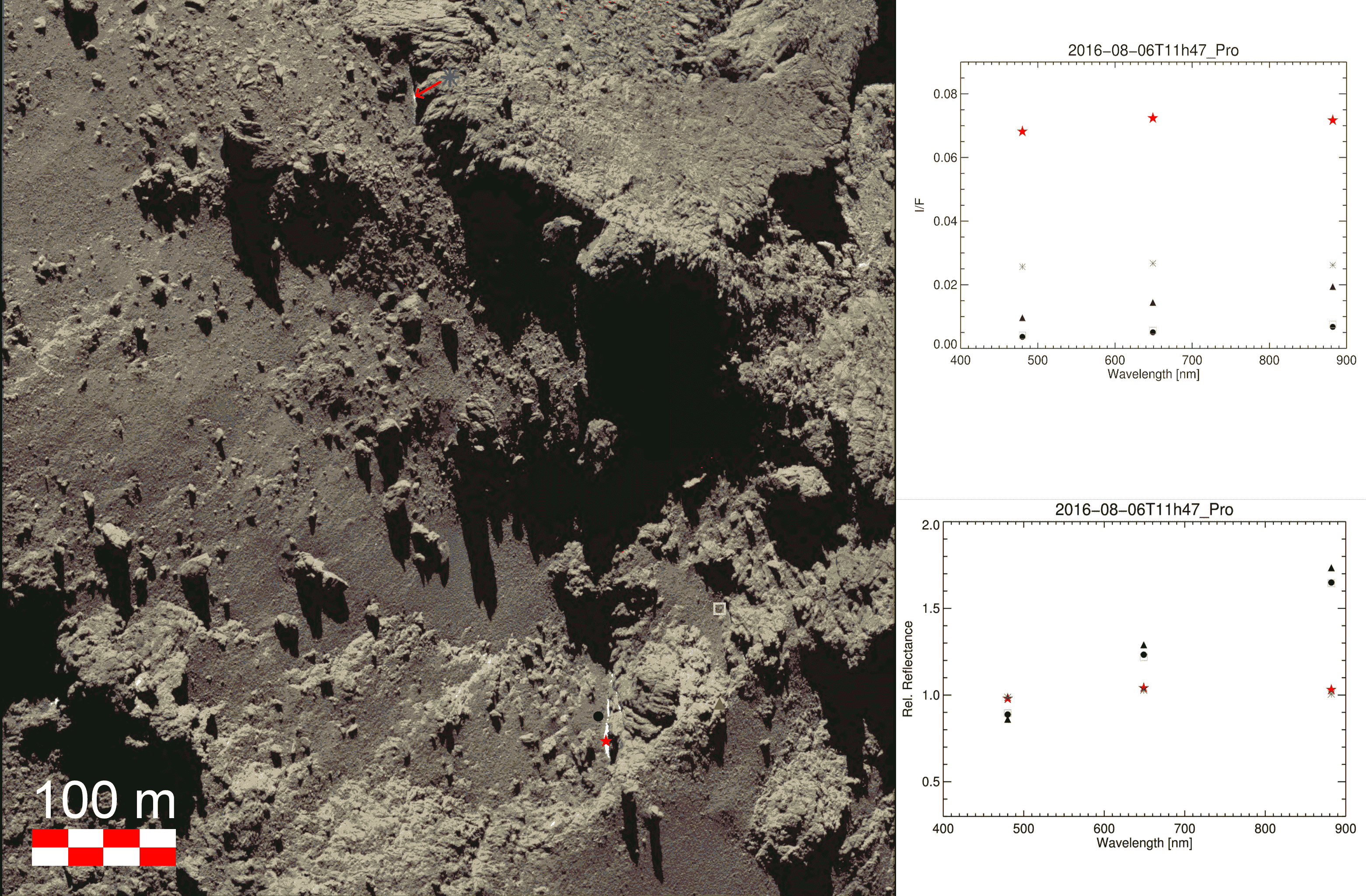
Figure 14: RGB reflectance properties of BF-06 and of another neighboring bright surface as observed in the NAC 2016-08-06T11:47 sequence of observations. The red star and blue asterisk indicate the bright feature at the bottom of an underhang close to UR-00 and BF-06, respectively. Other symbols mark neighboring smooth surfaces and consolidated material. In these observations, the phase angle is 71.4^∘and the resolution is 16 cm/px. For clarity, the area visible in this image is roughly delimited by the red square in fig. 8.

In this observation, the reflectance of the bright surfaces is clearly between 4 and 10 times higher than that of neighboring smooth surfaces of fine-material deposits, and it clearly exhibits a spectral behavior with a neutral slope with respect to the same neighboring surfaces. This observation therefore indicates the persistence of these bright surfaces, and in the paradigm of a spectral behavior consistent with a water-ice material enrichment, the lack of sufficient insolation to sublimate this material between April and August 2016. As the comet was at 3.5 au, it would then be quite likely that these surfaces would survive until the next approach to perihelion.

In the bright surfaces investigated conjointly by the OSIRIS and VIRTIS instruments, water-ice material is absolutely certain. However, the exact nature of the average terrain material that surrounds these bright features and composes the top-layer of the nucleus surface (also referred to as “dark terrain” in Fornasier et al., 2017) still remains to be defined.
Comparison of the photometric results from the February 2015 flyby with laboratory measurements has found that intra-mixture of carbon, tholins, and water ice (Jost et al., 2017a) matched the phase curve better than the inter-mixture counterpart. A similar observation was made regarding the nature of bright spots for this flyby observed with the OSIRIS/WAC camera (Hasselmann et al., 2017).
However, the comparison of these samples with the measurements of smooth fine-material deposits of the Ash-Imhotep transition had indicated a mismatch of these particular samples in terms of the spectral slopes, as tholinsinduced a stronger spectral slope than had been observed (see fig. 16 of Feller et al., 2016).

Recent researches into the spectrophotometric properties of cometary analogs have been notably reported in Jost et al. (2017a, b) and Rousseau et al. (2017). While the first study furthered the analysis of carbon, tholins, and water-ice mixtures, the latter investigated the properties of coal mixed with silicates and/or with pyrrhotites (iron sulfides).
In both studies, the authors have found mixtures that provided a satisfactory match of the comet spectrum in the 250-1000nm range. Additionally, Jost et al. (2017b) also reported mixtures that matched the observed phase-reddening phenomenon. However, Jost et al. (2017b) also noted that the investigated mixtures did not provide a simultaneous match of the comet albedo, spectrum, phase curve, and of the phase reddening.
Furthermore, Rousseau et al. (2017) noted that although they found mixtures that matched the comet reflectance, these mixtures did not match the observed spectral slope of the average comet terrain either. They pointed out that the organic compound they used induced a lower spectral slope than the one of the comet.

Consequently, investigations for an appropriate cometary analog for the surface of 67P in terms of spectrophotometric and physical properties, as pointed in part in Kaufmann and Hagermann (2018), for instance, are still ongoing.
In addition to considering the albedo and reflectance spectrum of a mixture, including phase-reddening measurements might prove a pertinent additional comparison factor. However, the grounds for this phenomenon are still the subject of research and remain to be well defined. This phenomenon has tentatively been attributed to the increased contribution of the multiple scattering at large phase angles as the wavelength and albedo increase, and to a contribution of surface roughness effects (Hapke, 2012; Sanchez et al., 2012 and Schröder et al., 2014). Jost et al. (2017a) further underlined that the nature of a surface phase reddening also appears to depend on its composition, and that in their surface analog mixtures, both the darkening agent (carbon particles) and the organic compound (tholins) had a distinctive influence on the presence and strength of the phase reddening.
While additional theoretical investigation and laboratory experiment validation are crucial to determine the frame of the phase-reddening phenomenon within a low temperature, irradiated and Van-der-Waals forces dominated environment, considering the phase reddening in current laboratory experiments would nevertheless constitute a further valuable comparison tool for determining an appropriate analog of the surface of 67P.

6 Conclusions

We have presented here the results of the geomorphological mapping and of the spectrophotometric analysis based on the OSIRIS/NAC images acquired during the April 2016 flyby manoeuvre above the Imhotep-Khepry transition area on 67P.

• We have identified and mapped the host of morphological units that are visible in the Khepry-Imhotep transition, which, without marking this region as unique, indicate its diversity and relative complexity.

• We have performed spectrophotometric analyses of the transition in general as well as of peculiar surface elements. While the smooth-looking regolith of this region is similar to the average dark terrain of the nucleus in terms of reflectance and spectral slope, rough terrains such as diamictons, degraded outcrops, and consolidated material exhibit a lower-than-average reflectance and a higher-than-average spectral slope.
  One particular outcrop of consolidated material roofed by a cuesta presents a slightly higher-than-average reflectance and a slightly lower-than-average spectral slope, which likely indicates a local compositional heterogeneity at a scale of some tens of meters.
  Additionally, some meter-sized features also present a peculiar spectrophotometric behavior. Sombre boulders, which are ubiquitous in the Imhotep-Khepry transition, show a similar spectral behavior as the neighboring smooth terrains, and their reflectance is $\sim$20% lower than average. The bright surfaces of this area are unmistakable, their reflectance is at least at twice the local average, and their spectral behavior is repeatedly less steep than the average surface. These features both indicate small-scale compositional heterogeneities across the surface of this region.

• We have identified that the bright features that exhibit moderate to neutral spectral slopes are likely candidates for locations that are enriched in water-ice material. We have also shown that some of the bright surfaces investigated in April 2016 that are likely enriched in water-ice material have persisted up to and beyond the frost line, and at least up to August 2016. This further supports evidence for long-term survival of water-ice-rich material and frosts on the nucleus surface.

• We have measured the local phase-reddening parameters as the comet was at 2.7 au outbound from perihelion, and have found them to be on the same order as those obtained for the Ash-Imhotep transition observed during the February 2015 flyby, which further indicates seasonal variations on the surface of the nucleus.

Accordingly, this transition area displays a diversity in reflectances and spectral slopes that is as great as it is in morphological terms. This indicates that the variety in the surface top-layer composition was greater than in the flyby area on 14 February 2015.

Appendix A Additional material

April 2016 (UTC)	NAC Filters	D (km)	Res. (m/px)	$\alpha_{m}$ (∘)	$\alpha_{min}$ - $\alpha_{max}$ (∘)	Longitude	Latitude
09T12:15:17.916	All filters	47.0$\pm$0.6	0.87$\pm$0.05	60.6	59.5-61.7	149.89∘	-5.76∘
09T23:01:09.919	F84, F82, F88	28.8$\pm$0.2	0.54$\pm$0.02	7.80	6.67-8.94	121.33∘	-17.09∘
09T23:08:09.910	”	28.8$\pm$0.2	0.54$\pm$0.02	6.99	5.85-8.14	118.12∘	-16.77∘
09T23:14:09.894	”	28.8$\pm$0.2	0.54$\pm$0.02	6.29	5.16-7.45	115.04∘	-16.64∘
09T23:19:08.951	”	28.8$\pm$0.2	0.53$\pm$0.02	5.72	4.58-6.87	112.54∘	-16.50∘
09T23:22:09.905	”	28.7$\pm$0.1	0.53$\pm$0.02	5.37	4.23-6.53	111.24∘	-16.29∘
09T23:25:09.886	”	28.7$\pm$0.1	0.53$\pm$0.02	5.02	3.88-6.19	109.92∘	-16.11∘
09T23:28:09.912	”	28.7$\pm$0.1	0.53$\pm$0.02	4.68	3.53-5.85	108.70∘	-15.87∘
09T23:31:09.942	”	28.7$\pm$0.1	0.53$\pm$0.01	4.34	3.19-5.50	107.51∘	-15.62∘
09T23:34:09.904	”	28.7$\pm$0.1	0.53$\pm$0.01	3.99	2.84-5.18	106.47∘	-14.71∘
09T23:37:09.883	”	28.7$\pm$0.1	0.53$\pm$0.01	3.65	2.48-4.88	105.35∘	-13.30∘
09T23:40:09.927	”	28.6$\pm$0.1	0.53$\pm$0.01	3.30	2.10-4.58	104.30∘	-11.19∘
09T23:43:09.884	”	28.6$\pm$0.1	0.53$\pm$0.01	2.94	1.69-4.26	103.33∘	-8.71∘
09T23:46:09.901	”	28.6$\pm$0.1	0.53$\pm$0.01	2.57	1.25-3.93	102.74∘	-5.78∘
09T23:49:09.982	”	28.6$\pm$0.1	0.53$\pm$0.01	2.19	0.80-3.56	103.48∘	-2.47∘
09T23:52:10.005	”	28.6$\pm$0.1	0.53$\pm$0.01	1.82	0.39-3.17	104.65∘	0.87∘
09T23:55:09.984	”	28.6$\pm$0.1	0.53$\pm$0.01	1.48	0.095*-2.79	106.05∘	3.32∘
09T23:58:09.911	”	28.6$\pm$0.1	0.53$\pm$0.01	1.24	0.095*-2.47	107.85∘	5.11∘
10T00:01:09.929	”	28.6$\pm$0.1	0.53$\pm$0.01	1.21	0.095*-2.43	110.21∘	5.88∘
10T00:04:09.927	”	28.6$\pm$0.1	0.53$\pm$0.01	1.42	0.095*-2.72	112.57∘	5.78∘
10T00:07:10.009	”	28.6$\pm$0.1	0.53$\pm$0.01	1.75	0.31-3.09	114.98∘	4.60∘
10T00:10:09.944	”	28.7$\pm$0.1	0.53$\pm$0.01	2.11	0.70-3.49	117.11∘	2.31∘
10T00:13:10.092	”	28.7$\pm$0.1	0.53$\pm$0.01	2.48	1.14-3.85	118.13∘	-0.52∘
10T00:16:08.998	”	28.8$\pm$0.1	0.53$\pm$0.01	2.84	1.57-4.18	118.36∘	-3.40∘
10T00:19:09.893	”	28.8$\pm$0.1	0.54$\pm$0.01	3.19	1.98-4.48	117.89∘	-6.17∘
10T00:22:09.912	”	28.8$\pm$0.2	0.54$\pm$0.01	3.54	2.36-4.78	116.89∘	-8.22∘
10T00:25:09.908	”	28.9$\pm$0.2	0.54$\pm$0.02	3.88	2.72-5.08	115.50∘	-9.78∘
10T00:28:09.931	”	28.9$\pm$0.2	0.54$\pm$0.02	4.21	3.06-5.38	113.83∘	-10.48∘
10T00:31:09.977	”	28.9$\pm$0.2	0.54$\pm$0.02	4.54	3.40-5.71	112.01∘	-10.51∘
10T00:34:09.905	”	28.9$\pm$0.2	0.54$\pm$0.02	4.88	3.73-6.04	110.17∘	-10.44∘
10T00:37:09.911	”	28.9$\pm$0.2	0.54$\pm$0.02	5.21	4.07-6.37	108.31∘	-10.26∘
10T00:40:09.924	”	29.0$\pm$0.2	0.54$\pm$0.02	5.54	4.40-6.70	106.39∘	-9.98∘
10T00:43:09.896	”	29.0$\pm$0.2	0.54$\pm$0.02	5.87	4.74-7.03	104.49∘	-9.66∘
10T00:46:09.944	”	29.0$\pm$0.2	0.54$\pm$0.02	6.21	5.07-7.46	102.60∘	-9.41∘
10T11:50:16.568	All filters	53.8$\pm$0.5	1.00$\pm$0.05	51.2	49.9-52.2	87.31∘	-14.82∘

Table 6: List of OSIRIS/NAC observations used in this study: in the table above, D is the median distance between spacecraft to imaged surface, $\alpha_{m}$ is the median phase angle, and the next column gives the amplitude of the phase angle values. The longitudes and latitudes are those of the NAC boresight in the Cheops frame (see the main text for details).

Feature	Long.	Lat.	23h34	23h46	00h01	23h34	23h46	00h01
	$\pm$0.1	$\pm$0.1	I/F at 649 nm (%)			Spectral slope (%/100 nm)
UR-00	-46.7	-8.3	5.3$\pm$0.1	5.6$\pm$0.1	6.4$\pm$0.1	17.7$\pm$0.2	18.0$\pm$0.5	18.3$\pm$0.2
BF-01	-56.5	-8.3	20.0$\pm$3.0			8.0$\pm$11.0
BF-02	-43.1	-27.8	9.0$\pm$0.6			7.0$\pm$1.5
BF-03	-46.0	-20.3	7.0$\pm$0.2	7.6$\pm$0.1		11.0$\pm$2.0	10.8$\pm$0.4
BF-04	-45.9	-20.4		8.8$\pm$0.3			8.5$\pm$0.6
BF-05	-45.7	-12.6	9.0$\pm$1.6	11.0$\pm$1.4	11.0$\pm$1.2	5.1$\pm$5.0	6.0$\pm$2.0	9.0$\pm$3.0
BF-06	-41.8	-6.9	9.0$\pm$1.0	11.0$\pm$1.2	14.0$\pm$1.7	7.0$\pm$3.0	5.0$\pm$5.0	5.0$\pm$4.0
BF-07	-39.0	-6.7	6.4$\pm$0.2	7.0$\pm$0.3	8.0$\pm$0.3	15.9$\pm$0.5	16.2$\pm$0.6	15.0$\pm$1.0
BF-08	-51.6	-4.3	12.0$\pm$1.3	11.0$\pm$1.1		2.3$\pm$1.5	4.0$\pm$1.1
BF-09	-54.2	-3.3			8.1$\pm$0.1			10.6$\pm$0.5
BF-10	-32.5	13.2			11.3$\pm$0.6			6.8$\pm$0.6
SB-00	-51.4	-24.9	4.2$\pm$0.1			20.1$\pm$0.7
SB-01	-43.9	-18.4	4.9$\pm$0.1	5.3$\pm$0.1		20.2$\pm$0.5	20.1$\pm$0.7
SB-02	-45.5	-11.7	4.8$\pm$0.1	5.2$\pm$0.1		21.1$\pm$0.5	21.8$\pm$0.4
SB-03	-27.7	-3.8	5.3$\pm$0.1	5.8$\pm$0.1		18.4$\pm$0.3	18.5$\pm$0.1
SB-04	-20.8	7.0	5.0$\pm$0.1	5.4$\pm$0.1		18.5$\pm$0.2	18.8$\pm$0.1
SB-05	-20.0	7.5	5.1$\pm$0.1	5.5$\pm$0.1	5.7$\pm$0.1	19.5$\pm$0.3	19.7$\pm$0.2	19.5$\pm$0.2
SB-06	-42.6	6.5		5.0$\pm$0.1	5.6$\pm$0.1		19.7$\pm$0.5	18.5$\pm$0.4
SB-07	-17.4	9.6			5.4$\pm$0.1			19.0$\pm$0.1

Table 7: Extended list of features investigated: In the table above, the first column indicates the ID of the feature, the second and third columns give the features’ positions relative to the Cheops boulder, the two sets of three columns list their reflectance at 649 nm and their spectral slopes in the 535-743 nm range for the three sequences of observations acquired close to the moment of opposition and discussed in the main text.

Properties	February 2015	April 2016
# NAC images	91	121
Filters used	24 sequences with F84,F82,F88	33 sequences with F84,F82,F88
	2 sequences with all filters	2 sequences with all filters
Sequences cadence (seconds)	36 - 600	180 - 420
Best pixel scale	0.11 m/pxl	0.53 m/pxl
Phase angle range	0∘- 33∘	0∘-12∘+ $\sim$ 51∘+ $\sim$ 60∘
Phase reddening	S(0∘) = 17.9%/100 nm	S(0∘) = 17.9%/100 nm
parameters	$\beta$ = 6.52 $\cdot$ 10${}^{-}4$/100nm/∘	$\beta$ = 6.40 $\cdot$ 10${}^{-}4$/100nm/∘
Median pv(0∘, 649 nm)	6.3%$\pm$0.6%	6.3%$\pm$0.6%
Max pv(0∘, 649 nm)	10.4%	16.0%*
Peculiar features	Strata heads,	bright patches,
	bright patches,	somber boulders
	somber boulders
Investigated surfaces
Bright patches	Spectral slope† > 17%/100nm	Spectral slope† < 10%/100nm
Sombre boulders	Spectral slope†> 17%/100nm	Spectral slope† > 17%/100nm
Spectral differences	Slight	Strong
(bright/somber features)
Bright features’ spectral	average dark terrain	water-ice rich material
behavior similar to
Favored locations of bright features	None obvious	Bottom of niches and underhangs

Table 8: Comparison of the main characteristics of the February 2015 and April 2016 flybys: Abridged comparative of the two flybys discussed in Feller et al. (2016) and in the main text.
$\dagger$: Spectral slope close to 0^∘of phase angle.

References

- Agarwal et al. (2017) Agarwal, J., Della Corte, V., Feldman, P. D., et al.: 2017, Monthly Notices of the Royal Astronomical Society 469(Suppl. 2), s606
- Auger et al. (2015) Auger, A.-T., Groussin, O., Jorda, L., et al.: 2015, Astronomy and Astrophysics 583, A35
- Bar-Nun et al. (1993) Bar-Nun, A., Barucci, M., Bussoletti, E., et al.: 1993, ROSETTA Comet Rendezvous Mission, Technical report, ESA
- Barucci et al. (2016) Barucci, M. A., Filacchione, G., Fornasier, S., et al.: 2016, Astronomy and Astrophysics 595, A102
- Bessell (1990) Bessell, M. S.: 1990, Publications of the Astronomical Society of the Pacific 102, 1181
- Bugeau and Pérez (2009) Bugeau, A. and Pérez, P.: 2009, Computer Vision and Image Understanding 113(4), 459
- Capaccioni et al. (2015) Capaccioni, F., Coradini, A., Filacchione, G., et al.: 2015, Science 347(1), aaa0628
- Clark et al. (2002) Clark, B. E., Hapke, B., Pieters, C., and Britt, D.: 2002, Asteroids III pp 585–599
- Coradini et al. (2007) Coradini, A., Capaccioni, F., Drossart, P., et al.: 2007, Space Science Reviews 128, 529
- Deshapriya et al. (2016) Deshapriya, J. D. P., Barucci, M. A., Fornasier, S., et al.: 2016, Monthly Notices of the Royal Astronomical Society 462, S274
- Deshapriya et al. (2018) Deshapriya, J. D. P., Barucci, M. A., Fornasier, S., et al.: 2018, Astronomy and Astrophysics 613, A36
- El-Maarry et al. (2015) El-Maarry, M. R., Thomas, N., Giacomini, L., et al.: 2015, Astronomy and Astrophysics 583, A26
- El-Maarry et al. (2016) El-Maarry, M. R., Thomas, N., Gracia-Berná, A., et al.: 2016, Astronomy and Astrophysics 593, A110
- Fairbairn (2005) Fairbairn, M. B.: 2005, Journal of the Royal Astronomical Society of Canada 99, 92
- Feller et al. (2016) Feller, C., Fornasier, S., Hasselmann, P. H., et al.: 2016, Monthly Notices of the Royal Astronomical Society 462, S287
- Filacchione et al. (2016a) Filacchione, G., Capaccioni, F., Ciarniello, M., et al.: 2016a, Icarus 274, 334
- Filacchione et al. (2016b) Filacchione, G., de Sanctis, M. C., Capaccioni, F., et al.: 2016b, Nature 529, 368
- Fornasier et al. (2017) Fornasier, S., Feller, C., Lee, J.-C., et al.: 2017, Monthly Notices of the Royal Astronomical Society 469, S93
- Fornasier et al. (2015) Fornasier, S., Hasselmann, P. H., Barucci, M. A., et al.: 2015, Astronomy and Astrophysics 583, A30
- Fornasier et al. (ssue) Fornasier, S., Hoang, V., Hasselmann, P., et al.: this issue, A&A
- Fornasier et al. (2016) Fornasier, S., Mottola, S., Keller, H. U., et al.: 2016, Science 354, 1566
- Gaskell et al. (2008) Gaskell, R. W., Barnouin-Jha, O. S., Scheeres, D. J., et al.: 2008, Meteoritics and Planetary Science 43, 1049
- Gehrels et al. (1964) Gehrels, T., Coffeen, T., and Owings, D.: 1964, Astronomical Journal 69
- Giacomini et al. (2016) Giacomini, L., Massironi, M., Thomas, N., et al.: 2016, Memorie della Societa Astronomica Italiana 87, 159
- Gradie et al. (1980) Gradie, J., Veverka, J., and Buratti, B.: 1980, in S. A. Bedini (ed.), Lunar and Planetary Science Conference Proceedings, Vol. 11 of Lunar and Planetary Science Conference Proceedings, pp 799–815
- Groussin et al. (2015) Groussin, O., Sierks, H., Barbieri, C., et al.: 2015, Astronomy and Astrophysics 583, A36
- Hapke (1993) Hapke, B.: 1993, Theory of reflectance and emittance spectroscopy, Cambridge University Press, 2 edition
- Hapke (2012) Hapke, B.: 2012, Icarus 221, 1079
- Hasselmann et al. (2017) Hasselmann, P. H., Barucci, M. A., Fornasier, S., et al.: 2017, Monthly Notices of the Royal Astronomical Society 469, S550
- Jewitt and Meech (1986) Jewitt, D. and Meech, K. J.: 1986, Astrophysical Journal 310, 937
- Jorda et al. (2010) Jorda, L., Spjuth, S., Keller, H. U., Lamy, P., and Llebaria, A.: 2010, in Computational Imaging VIII, Vol. 7533 of Proceedings of the International Society for Optical Engineering, p. 753311
- Jost et al. (2017a) Jost, B., Pommerol, A., Poch, O., et al.: 2017a, Planetary Space Sciences 148, 1
- Jost et al. (2017b) Jost, B., Pommerol, A., Poch, O., et al.: 2017b, Planetary Space Sciences 145, 14
- Kaufmann and Hagermann (2018) Kaufmann, E. and Hagermann, A.: 2018, Icarus 311, 105
- Keller et al. (2007) Keller, H. U., Barbieri, C., Lamy, P., et al.: 2007, Space Science Reviews 128(1), 433
- Keller et al. (2015) Keller, H. U., Mottola, S., Davidsson, B., et al.: 2015, Astronomy and Astrophysics 583, A34
- Knollenberg et al. (2016) Knollenberg, J., Lin, Z. Y., Hviid, S. F., et al.: 2016, Astronomy and Astrophysics 596, A89
- Küppers et al. (2007) Küppers, M., Mottola, S., Lowry, S. C., et al.: 2007, Astronomy and Astrophysics 462, L13
- La Forgia et al. (2015) La Forgia, F., Giacomini, L., Lazzarin, M., et al.: 2015, Astronomy and Astrophysics 583, A41
- Lee et al. (2016) Lee, J.-C., Massironi, M., Ip, W.-H., et al.: 2016, Monthly Notices of the Royal Astronomical Society 462, S573
- Lucas and Kanade (1981) Lucas, B. D. and Kanade, T.: 1981, in Proceedings of the 7th International Joint Conference on Artificial Intelligence (IJCAI ’81), pp 674–679
- Massironi et al. (2015) Massironi, M., Simioni, E., Marzari, F., et al.: 2015, Nature 526, 402
- Oklay et al. (2017) Oklay, N., Mottola, S., Vincent, J.-B., et al.: 2017, Monthly Notices of the Royal Astronomical Society 469, S582
- Oklay et al. (2016a) Oklay, N., Sunshine, J. M., Pajola, M., et al.: 2016a, Monthly Notices of the Royal Astronomical Society 462, S394
- Oklay et al. (2016b) Oklay, N., Vincent, J.-B., Fornasier, S., et al.: 2016b, Astronomy and Astrophysics 586, A80
- Pajola et al. (2016) Pajola, M., Oklay, N., La Forgia, F., et al.: 2016, Astronomy and Astrophysics 592, A69
- Penasa et al. (2017) Penasa, L., Massironi, M., Naletto, G., et al.: 2017, Monthly Notices of the Royal Astronomical Society 469, S741
- Pommerol et al. (2015) Pommerol, A., Jost, B., Poch, O., et al.: 2015, Planetary Space Sciences 109, 106
- Poulet et al. (2016) Poulet, F., Lucchetti, A., Bibring, J.-P., et al.: 2016, Monthly Notices of the Royal Astronomical Society 462, S23
- Preusker et al. (2015) Preusker, F., Scholten, F., Matz, K.-D., et al.: 2015, Astronomy and Astrophysics 583, A33
- Preusker et al. (2017) Preusker, F., Scholten, F., Matz, K.-D., et al.: 2017, A&A 607, L1
- Quirico et al. (2016) Quirico, E., Moroz, L. V., Schmitt, B., et al.: 2016, Icarus 272, 32
- Raponi et al. (2016) Raponi, A., Ciarniello, M., Capaccioni, F., et al.: 2016, Monthly Notices of the Royal Astronomical Society 462, S476
- Rousseau et al. (2017) Rousseau, B., Érard, S., Beck, P., et al.: 2017, Icarus
- Rublee et al. (2011) Rublee, E., Rabaud, V., Konolige, K., and Bradski, G.: 2011, in 2011 International Conference on Computer Vision, pp 2564–2571
- Sanchez et al. (2012) Sanchez, J. A., Reddy, V., Nathues, A., et al.: 2012, Icarus 220, 36
- Schröder et al. (2014) Schröder, S. E., Grynko, Y., Pommerol, A., et al.: 2014, Icarus 239, 201
- Seeliger (1885) Seeliger, H.: 1885, Astronomische Nachrichten 110, 385
- Shi and Tomasi (1994) Shi, J. and Tomasi, C.: 1994, pp 593–600
- Shkuratov et al. (2011) Shkuratov, Y., Kaydash, V., Korokhin, V., et al.: 2011, Planetary Space Sciences 59, 1326
- Sierks et al. (2015) Sierks, H., Barbieri, C., Lamy, P. L., et al.: 2015, Science 347(1), aaa1044
- Sunshine et al. (2006) Sunshine, J. M., A’Hearn, M. F., Groussin, O., et al.: 2006, Science 311, 1453
- Thomas et al. (2015a) Thomas, N., Davidsson, B., El-Maarry, M. R., et al.: 2015a, Astronomy and Astrophysics 583, A17
- Thomas et al. (2015b) Thomas, N., Sierks, H., Barbieri, C., et al.: 2015b, Science 347(1), aaa0440
- Tubiana et al. (2015) Tubiana, C., Güttler, C., Kovacs, G., et al.: 2015, Astronomy and Astrophysics 583, A46
- van der Walt et al. (2014) van der Walt, S., Schönberger, J. L., Nunez-Iglesias, J., et al.: 2014, ArXiv e-prints